Use of UAS Multispectral Imagery at Different Physiological Stages for Yield Prediction and Input Resource Optimization in Corn


Abstract
:1. Introduction
2. Materials and Methods
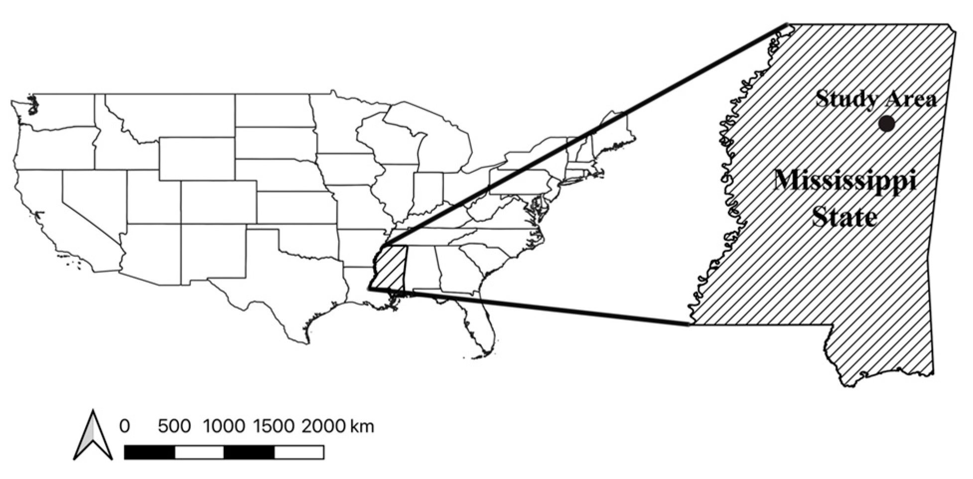
2.1. Study Area
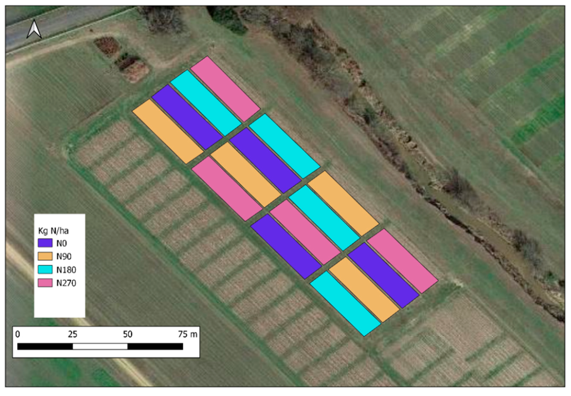
2.2. Experimental Design
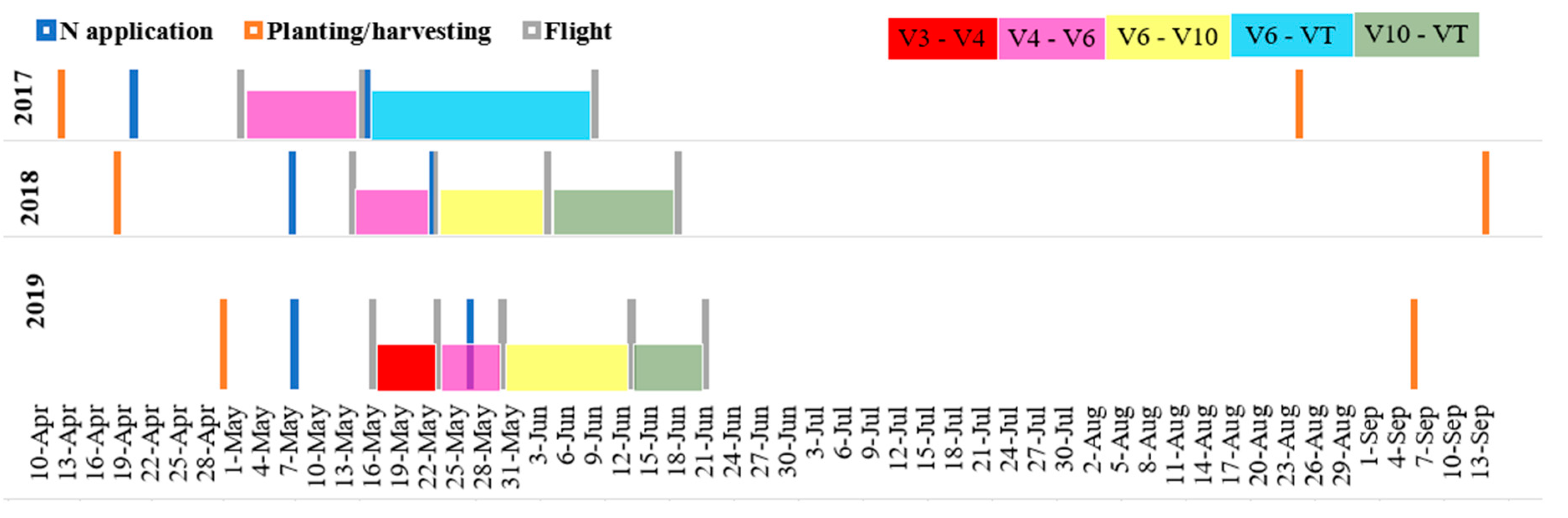
2.3. Data Collection
2.3.1. Vegetation Indices
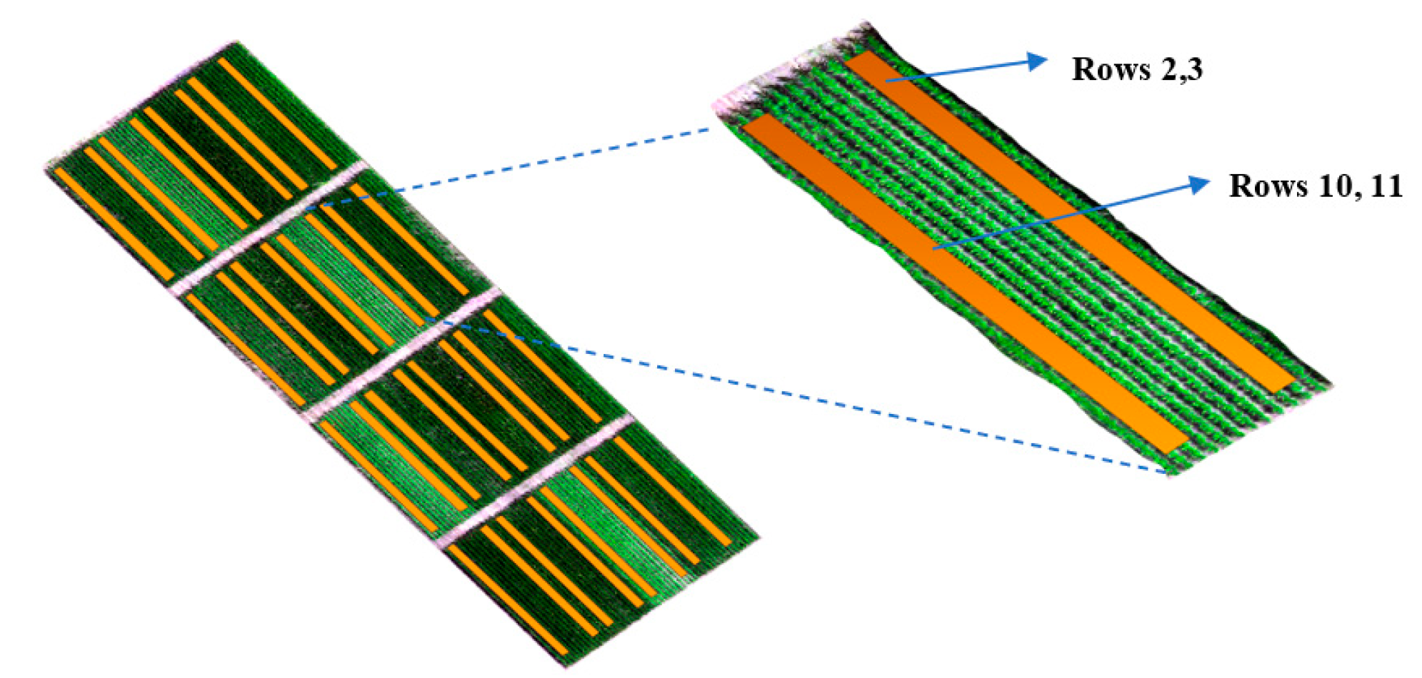
2.3.2. Masking Soil Pixels
2.3.3. Harvesting Process
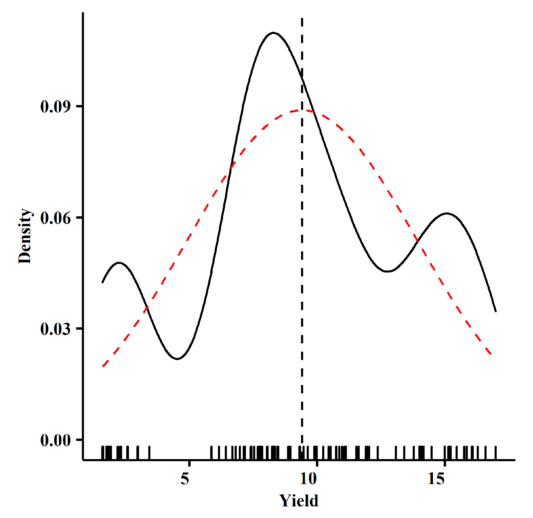
2.4. Outlier Detection
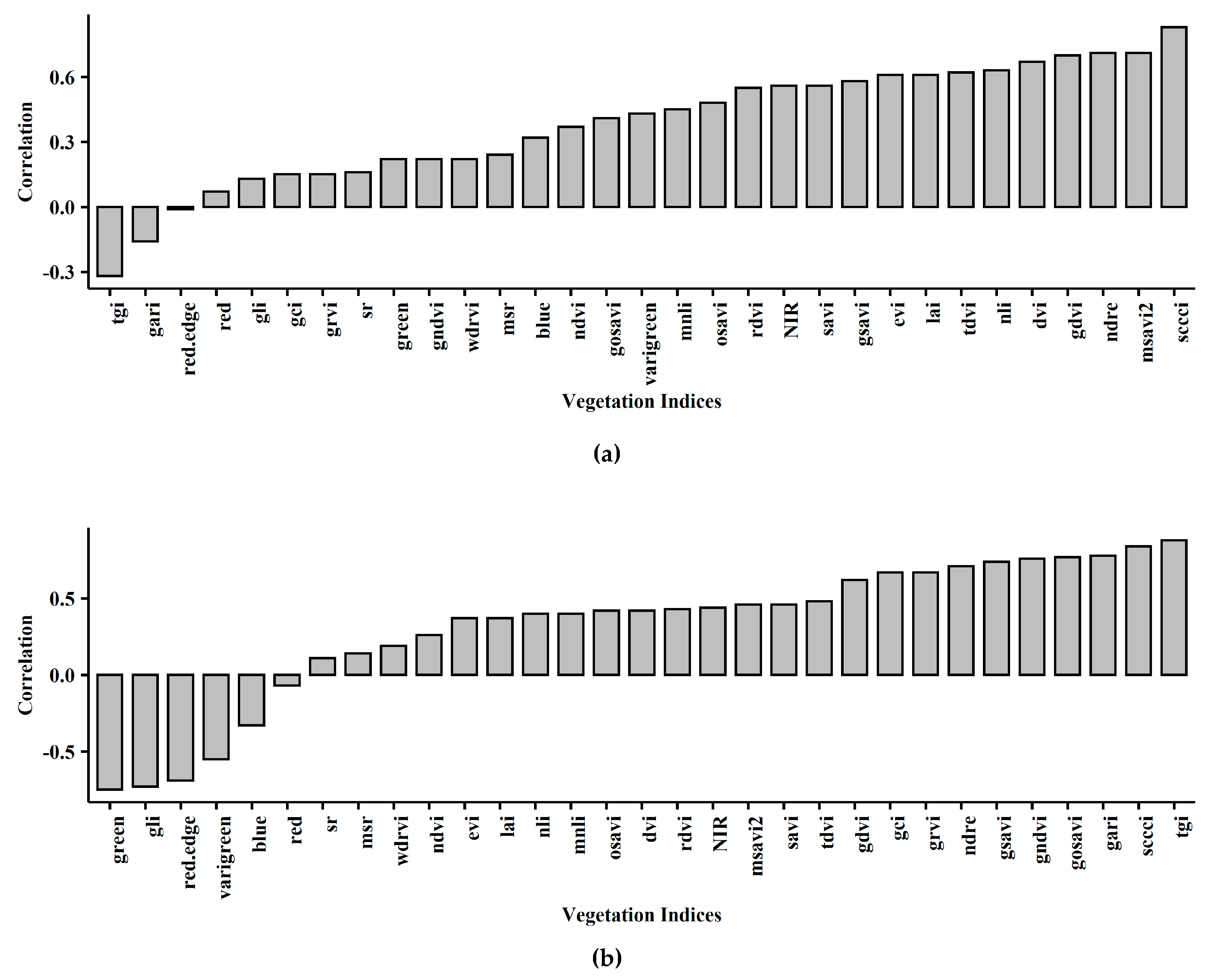
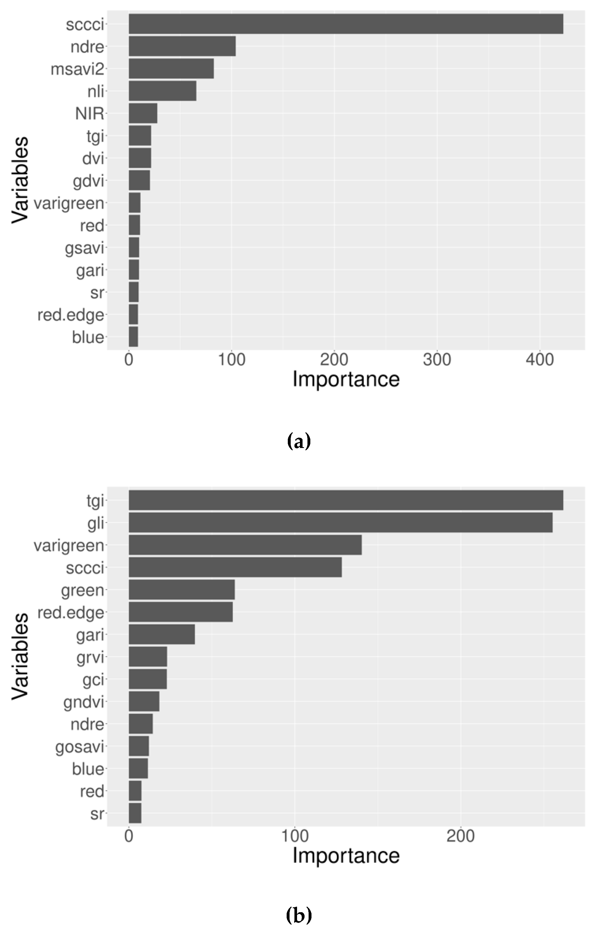
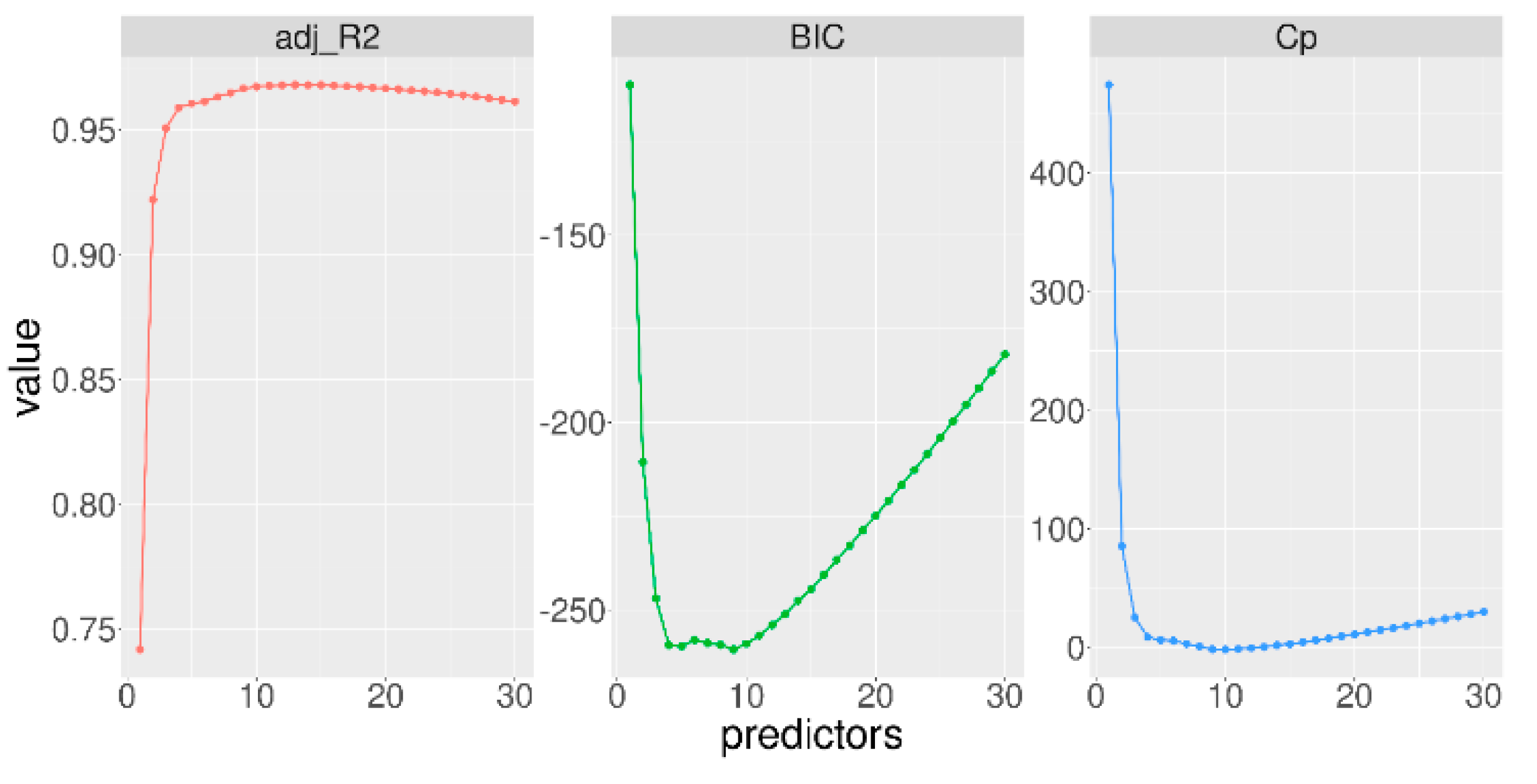
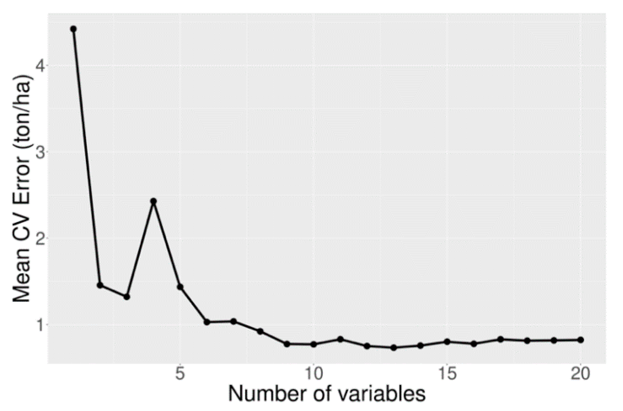
2.5. Feature Selection
2.6. Statistical Analysis
3. Results and Discussion
4. Conclusions
Author Contributions
Funding
Acknowledgments
Conflicts of Interest
References
- Rouse, J.W.; Hass, R.H.; Schell, J.A.; Deering, D.W.; Harlan, J.C. Monitoring the Vernal Advancement and Retrogradation (GreenWave Effect) of Natural Vegetation [Great Plains Corridor]; NASA: Washington, DC, USA, 1974. [Google Scholar]
- Santamar, L. Modeling Biomass Production in Seasonal Wetlands Using MODIS NDVI Land Surface Phenology. Remote Sens. 2017, 9, 392. [Google Scholar] [CrossRef] [Green Version]
- Hogrefe, K.R.; Patil, V.P.; Ruthrauff, D.R.; Meixell, B.W.; Budde, M.E.; Hupp, J.W.; Ward, D.H. Normalized Difference Vegetation Index as an Estimator for Abundance and Quality of Avian Herbivore Forage in Arctic Alaska. Remote Sens. 2017, 9, 1234. [Google Scholar] [CrossRef] [Green Version]
- Bronson, K.F.; Booker, J.D.; Keeling, J.W.; Boman, R.K.; Wheeler, T.A.; Lascano, R.J.; Nichols, R.L. Cotton Canopy Reflectance at Landscape Scale as Affected by Nitrogen Fertilization. Agron. J. 2005, 97, 654–660. [Google Scholar] [CrossRef]
- Chen, J.M. Evaluation of Vegetation Indices and a Modified Simple Ratio for Boreal Applications. Can. J. Remote Sens. 1996, 22, 229–242. [Google Scholar] [CrossRef]
- Jackson, R.D.; Huete, A.R. Interpreting Vegetation Indices. Prev. Vet. Med. 1991, 11, 185–200. [Google Scholar] [CrossRef]
- Báez-González, A.D.; Chen, P.Y.; Tiscareño-López, M.; Srinivasan, R. Using Satellite and Field Data with Crop Growth Modeling to Monitor and Estimate Corn Yield in Mexico. Crop Sci. 2002, 42, 1943–1949. [Google Scholar] [CrossRef]
- Shiu, Y.S.; Chuang, Y.C. Yield Estimation of Paddy Rice Based on Satellite Imagery: Comparison of Global and Local Regression Models. Remote Sens. 2019, 11, 111. [Google Scholar] [CrossRef] [Green Version]
- Silvestro, P.C.; Pignatti, S.; Pascucci, S.; Yang, H.; Li, Z.; Yang, G.; Huang, W.; Casa, R. Estimating Wheat Yield in China at the Field and District Scale from the Assimilation of Satellite Data into the Aquacrop and Simple Algorithm for Yield (SAFY) Models. Remote Sens. 2017, 9, 509. [Google Scholar] [CrossRef] [Green Version]
- Sharma, L.K.; Bu, H.; Denton, A.; Franzen, D.W. Active-Optical Sensors Using Red NDVI Compared to Red Edge NDVI for Prediction of Corn Grain Yield in North Dakota, U.S.A. Sensors 2015, 15, 27832–27853. [Google Scholar] [CrossRef]
- Wang, T.; Shi, J.; Letu, H.; Ma, Y.; Li, X.; Zheng, Y. Detection and Removal of Clouds and Associated Shadows in Satellite Imagery Based on Simulated Radiance Fields. J. Geophys. Res. Atmos. 2019, 124, 7207–7225. [Google Scholar] [CrossRef] [Green Version]
- Bondi, E.; Salvaggio, C.; Montanaro, M.; Gerace, A.D. Calibration of UAS Imagery Inside and Outside of Shadows for Improved Vegetation Index Computation. In Autonomous Air and Ground Sensing Systems for Agricultural Optimization and Phenotyping, Proceedings of the SPIE, Baltimore, MD, USA, 17–26 May 2016; SPIE: Bellingham, WA, USA, 2016; Volume 9866. [Google Scholar] [CrossRef]
- Zhang, C.; Kovacs, J.M. The Application of Small Unmanned Aerial Systems for Precision Agriculture: A Review. Precis. Agric. 2012, 13, 693–712. [Google Scholar] [CrossRef]
- Iizuka, K.; Itoh, M.; Shiodera, S.; Matsubara, T.; Dohar, M.; Watanabe, K. Advantages of Unmanned Aerial Vehicle (UAV) Photogrammetry for Landscape Analysis Compared with Satellite Data: A Case Study of Postmining Sites in Indonesia. Cogent Geosci. 2018, 4, 1498180. [Google Scholar] [CrossRef]
- Gnädinger, F.; Schmidhalter, U. Digital Counts of Maize Plants by Unmanned Aerial Vehicles (UAVs). Remote Sens. 2017, 9, 544. [Google Scholar] [CrossRef] [Green Version]
- Qin, Z.; Myers, D.B.; Ransom, C.J.; Kitchen, N.R.; Liang, S.Z.; Camberato, J.J.; Carter, P.R.; Ferguson, R.B.; Fernandez, F.G.; Franzen, D.W.; et al. Application of Machine Learning Methodologies for Predicting Corn Economic Optimal Nitrogen Rate. Agron. J. 2018, 110, 2596–2607. [Google Scholar] [CrossRef] [Green Version]
- Khanal, S.; Fulton, J.; Klopfenstein, A.; Douridas, N.; Shearer, S. Integration of High Resolution Remotely Sensed Data and Machine Learning Techniques for Spatial Prediction of Soil Properties and Corn Yield. Comput. Electron. Agric. 2018, 153, 213–225. [Google Scholar] [CrossRef]
- Natekin, A.; Knoll, A. Gradient Boosting Machines, a Tutorial. Front. Neurorobot. 2013, 7. [Google Scholar] [CrossRef] [Green Version]
- Gitelson, A.A. Wide Dynamic Range Vegetation Index for Remote Quantification of Biophysical Characteristics of Vegetation. J. Plant Physiol. 2004, 161, 165–173. [Google Scholar] [CrossRef] [Green Version]
- Gitelson, A.A.; Kaufman, Y.J.; Stark, R.; Rundquist, D. Novel Algorithms for Remote Estimation of Vegetation Fraction. Remote Sens. Environ. 2002, 80, 76–87. [Google Scholar] [CrossRef] [Green Version]
- Erdle, K.; Mistele, B.; Schmidhalter, U. Field Crops Research Comparison of Active and Passive Spectral Sensors in Discriminating Biomass Parameters and Nitrogen Status in Wheat Cultivars. Field Crops Res. 2011, 124, 74–84. [Google Scholar] [CrossRef]
- Shanahan, J.F.; Schepers, J.S.; Francis, D.D.; Varvel, G.E.; Wilhelm, W.W.; Tringe, J.M.; Schlemmer, M.R.; Major, D.J. Use of Remote-Sensing Imagery to Estimate Corn Grain Yield. Agron. J. 2001, 93, 583–589. [Google Scholar] [CrossRef] [Green Version]
- Barzin, R.; Shirvani, A.; Lotfi, H. Estimation of Daily Average Downward Shortwave Radiation from MODIS Data Using Principal Components Regression Method: Fars Province Case Study. Int. Agrophys. 2017, 31, 23–34. [Google Scholar] [CrossRef] [Green Version]
- González-audícana, M.; Saleta, J.L.; Catalán, R.G.; García, R. Fusion of Multispectral and Panchromatic Images Using Improved IHS and PCA Mergers Based on Wavelet Decomposition. IEEE Trans. Geosci. Remote Sens. 2004, 42, 1291–1299. [Google Scholar] [CrossRef]
- Tucker, C.J. Red and Photographic Infrared Linear Combinations for Monitoring Vegetation. Remote Sens. Environ. 1979, 8, 127–150. [Google Scholar] [CrossRef] [Green Version]
- Wu, W. The Generalized Difference Vegetation Index (GDVI) for Dryland Characterization. Remote Sens. 2014, 6, 1211–1233. [Google Scholar] [CrossRef] [Green Version]
- Roujean, J.L.; Breon, F.M. Estimating PAR Absorbed by Vegetation from Bidirectional Reflectance Measurements. Remote Sens. Environ. 1995, 51, 375–384. [Google Scholar] [CrossRef]
- Bannari, A.; Asalhi, H.; Teillet, P.M. Transformed Difference Vegetation Index (TDVI) for Vegetation Cover Mapping. In Proceedings of the IEEE International Geoscience and Remote Sensing Symposium, Toronto, ON, Canada, 24–28 June 2002; Volume 5, pp. 3053–3055. [Google Scholar] [CrossRef]
- Pathak, R.; Barzin, R.; Bora, G.C. Data-Driven Precision Agricultural Applications Using Field Sensors and Unmanned Aerial Vehicle. Int. J. Precis. Agric. Aviat. 2018, 1, 19–23. [Google Scholar] [CrossRef] [Green Version]
- Gitelson, A.A.; Merzlyak, M.N. Remote Estimation of Chlorophyll Content in Higher Plant Leaves. Int. J. Remote Sens. 1998, 18, 2691–2697. [Google Scholar] [CrossRef]
- Gitelson, A.A.; Merzlyak, M.N. Quantitative Estimation of Chlorophyll-a Using Reflectance Spectra: Experiments with Autumn Chestnut and Maple Leaves. J. Photochem. Photobiol. 1994, 22, 247–252. [Google Scholar] [CrossRef]
- Raper, T.B.; Varco, J.J. Canopy-Scale Wavelength and Vegetative Index Sensitivities to Cotton Growth Parameters and Nitrogen Status. Precis. Agric. 2015, 16, 62–76. [Google Scholar] [CrossRef] [Green Version]
- Matsushita, B.; Yang, W.; Chen, J.; Onda, Y.; Qiu, G. Sensitivity of the Enhanced Vegetation Index (EVI) and Normalized Difference Vegetation Index (NDVI) to Topographic Effects: A Case Study in High-Density Cypress Forest. Sensors 2007, 7, 2636–2651. [Google Scholar] [CrossRef] [Green Version]
- Broge, N.H.; Leblanc, E. Comparing Prediction Power and Stability of Broadband and Hyperspectral Vegetation Indices for Estimation of Green Leaf Area Index and Canopy Chlorophyll Density. Remote Sens. Environ. 2001, 76, 156–172. [Google Scholar] [CrossRef]
- Gitelson, A.A.; Kaufman, Y.J.; Merzlyak, M.N. Use of a Green Channel in Remote Sensing of Global Vegetation from EOS- MODIS. Remote Sens. Environ. 1996, 58, 289–298. [Google Scholar] [CrossRef]
- Gitelson, A.A.; Gritz, Y.; Merzlyak, M.N. Relationships between Leaf Chlorophyll Content and Spectral Reflectance and Algorithms for Non-Destructive Chlorophyll Assessment in Higher Plant Leaves. J. Plant Physiol. 2003, 160, 271–282. [Google Scholar] [CrossRef]
- Louhaichi, M.; Borman, M.M.; Johnson, D.E. Spatially Located Platform and Aerial Photography for Documentation of Grazing Impacts on Wheat. Geocarto Int. 2001, 16, 65–70. [Google Scholar] [CrossRef]
- Raymond Hunt, E.; Daughtry, C.S.T.; Eitel, J.U.H.; Long, D.S. Remote Sensing Leaf Chlorophyll Content Using a Visible Band Index. Agron. J. 2011, 103, 1090–1099. [Google Scholar] [CrossRef] [Green Version]
- Vescovo, L.; Gianelle, D. Using the MIR Bands in Vegetation Indices for the Estimation of Grassland Biophysical Parameters from Satellite Remote Sensing in the Alps Region of Trentino (Italy). Adv. Space Res. 2008, 41, 1764–1772. [Google Scholar] [CrossRef]
- Gong, P.; Pu, R.; Biging, G.S.; Larrieu, M.R. Estimation of Forest Leaf Area Index Using Vegetation Indices Derived from Hyperion Hyperspectral Data. IEEE Trans. Geosci. Remote Sens. 2003, 41, 1355–1362. [Google Scholar] [CrossRef] [Green Version]
- Feng, W.; Wu, Y.; He, L.; Ren, X.; Wang, Y.; Hou, G.; Wang, Y.; Liu, W.; Guo, T. An Optimized Non-Linear Vegetation Index for Estimating Leaf Area Index in Winter Wheat. Precis. Agric. 2019, 20, 1157–1176. [Google Scholar] [CrossRef] [Green Version]
- Rondeaux, G.; Steven, M.; Baret, F. Optimization of Soil-Adjusted Vegetation Indices. Remote Sens. Environ. 1996, 55, 95–107. [Google Scholar] [CrossRef]
- Sripada, R.P.; Schmidt, J.P.; Dellinger, A.E.; Beegle, D.B. Evaluating Multiple Indices from a Canopy Reflectance Sensor to Estimate Corn N Requirements. Agron. J. 2008, 100, 1553–1561. [Google Scholar] [CrossRef]
- Qi, J.; Chehbouni, A.; Huete, A.R.; Kerr, Y.H.; Sorooshian, S. A Modify Soil Adjust Vegetation Index. Remote Sens. Environ. 1994, 126, 119–126. [Google Scholar] [CrossRef]
- Fraser, R.H.; Latifovic, R. Mapping Insect-Induced Tree Defoliation and Mortality Using Coarse Spatial Resolution Satellite Imagery. Int. J. Remote Sens. 2005, 26, 193–200. [Google Scholar] [CrossRef]
- Morales, A.; Nielsen, R.; Camberato, J. Effects of Removing Background Soil and Shadow Reflectance Pixels from RGB and NIR-Based Vegetative Index Maps. In Proceedings of the Purdue GIS Day, Purdue University, West Lafayette, IN, USA, 7 November 2019. [Google Scholar]
- Sader, S.A.; Winne, J.C. RGB-NDVI Colour Composites for Visualizing Forest Change Dynamics. Int. J. Remote Sens. 1992, 13, 3055–3067. [Google Scholar] [CrossRef]
- Gallo, B.C.; Demattê, J.A.M.; Rizzo, R.; Safanelli, J.L.; Mendes, W.d.S.; Lepsch, I.F.; Sato, M.V.; Romero, D.J.; Lacerda, M.P.C. Multi-Temporal Satellite Images on Topsoil Attribute Quantification and the Relationship with Soil Classes and Geology. Remote Sens. 2018, 10, 1571. [Google Scholar] [CrossRef]
- Torres, J.M.; Nieto, P.J.G.; Alejano, L.; Reyes, A.N. Detection of Outliers in Gas Emissions from Urban Areas Using Functional Data Analysis. J. Hazard. Mater. 2011, 186, 144–149. [Google Scholar] [CrossRef]
- Schubert, E.; Kriegel, H. Generalized Outlier Detection with Flexible Kernel Density Estimates. In Proceedings of the 2014 SIAM International Conference on Data Mining, Philadelphia, PA, USA, 24–26 April 2014; Society for Industrial and Applied Mathematics: Philadelphia, PA, USA, 2014; pp. 542–550. [Google Scholar]
- Nurunnabi, A.; West, G.; Belton, D. Outlier Detection and Robust Normal-Curvature Estimation in Mobile Laser Scanning 3D Point Cloud Data. Pattern Recognit. 2015, 48, 1404–1419. [Google Scholar] [CrossRef] [Green Version]
- Janitza, S.; Tutz, G.; Boulesteix, A.L. Random Forest for Ordinal Responses: Prediction and Variable Selection. Comput. Stat. Data Anal. 2016, 96, 57–73. [Google Scholar] [CrossRef]
- Breiman, L. Random Forests. Mach. Learn. 2001, 45, 5–32. [Google Scholar] [CrossRef] [Green Version]
- Kox, M.A.R.; Lüke, C.; Fritz, C.; van den Elzen, E.; van Alen, T.; Op den Camp, H.J.M.; Lamers, L.P.M.; Jetten, M.S.M.; Ettwig, K.F. Effects of Nitrogen Fertilization on Diazotrophic Activity of Microorganisms Associated with Sphagnum Magellanicum. Plant Soil 2016, 406, 83–100. [Google Scholar] [CrossRef] [Green Version]
- Akbarzadeh Baghban, A.; Younespour, S.; Jambarsang, S.; Yousefi, M.; Zayeri, F.; Azizi Jalilian, F. How to Test Normality Distribution for a Variable: A Real Example and a Simulation Study. J. Paramed. Sci. 2013, 4, 2008–4978. [Google Scholar]
- Vellidis, G.; Tucker, M.; Perry, C.; Reckford, D.; Butts, C.; Henry, H.; Liakos, V.; Hill, R.W.; Edwards, W. A Soil Moisture Sensor-Based Variable Rate Irrigation Scheduling System. In Precision Agriculture ‘13; Wageningen Academic Publishers: Wageningen, The Netherlands, 2013. [Google Scholar]
- Razali, N.M.; Wah, Y.B. Power Comparisons of Shapiro-Wilk, Kolmogorov-Smirnov, Lilliefors and Anderson-Darling Tests. J. Stat. Model. Anal. 2011, 2, 21–33. [Google Scholar] [CrossRef] [Green Version]
- Ghasemi, A.; Zahediasl, S. Normality Tests for Statistical Analysis: A Guide for Non-Statisticians. Int. J. Endocrinol. Metab. 2012, 10, 486–489. [Google Scholar] [CrossRef] [PubMed] [Green Version]
- Friedman, J.H. Stochastic Gradient Boosting. Comput. Stat. Data Anal. 2002, 38, 367–378. [Google Scholar] [CrossRef]
- Hastie, T.; Tibshirani, R.; Jerome, F. The Elements of Statistical Learning: Data Mining, Inference and Prediction; Springer Science & Business Media: Berlin, Germany, 2004. [Google Scholar]
- Kutner, M.H.; Nachtsheim, C.J.; Neter, J.; Li, W. Applied Linear Statistical Models, 5th ed.; McGraw-Hill Irwin: New York, NY, USA, 2005. [Google Scholar]
- Environmental Systems Research Institute ESRI. ArcGIS Desktop: Release 10. Redlands, CA, USA, Using ArcMap. 2019. Available online: https://qgis.org/en/site/ (accessed on 22 July 2020).
- QGIS Development Team: 2020. QGIS.org (2020). QGIS Geographic Information System. Open Source Geospatial Foundation Project. Available online: https://www.esri.com/news/arcnews/spring12articles/introducing-arcgis-101.html (accessed on 22 July 2020).
- R Core Team. A Language and Environment for Statistical Computing: R Foundation for Statistical Computing; R Core Team: Vienna, Austria, 2019. [Google Scholar]
- Hatfield, J.L.; Prueger, J.H. Value of Using Different Vegetative Indices to Quantify Agricultural Crop Characteristics at Different Growth Stages under Varying Management Practices. Remote Sens. 2010, 2, 562–578. [Google Scholar] [CrossRef] [Green Version]
- Trotter, T.F.; Frazier, P.S.; Trotter, M.G.; Lamb, D.W. Objective Biomass Assessment Using an Active Plant Sensor (Crop Circle), Preliminary Experiences on a Variety of Agricultural Landscapes. In Proceedings of the Ninth International Conference on Precision Agriculture’, Denver, CO, USA, 20–23 July 2008; Khosla, R., Ed.; Colorado State University: Fort Collins, CO, USA, 2008. [Google Scholar]
- Rattanakaew, T. Utilization of Canopy Reflectance to Predict Yield Response of Corn and Cotton to Varying Nitrogen Rates; Mississippi State University: Starkville, MS, USA, 2015. [Google Scholar]
- Kizil, Ü.; Genç, L.; İnalpulat, M.; Şapolyo, D.; Mİrİk, M. Lettuce (Lactuca Sativa L.) Yield Prediction under Water Stress Using Artificial Neural Network (ANN) Model and Vegetation Indices. Žemdirbystė= Agriculture 2012, 99, 409–418. [Google Scholar]


| Vegetation Indices (VI) | Name | Formula | Study Groups (Reference) | |
|---|---|---|---|---|
| 1 | DVI | Difference Vegetation Index | NIR − Reds | [25] |
| 2 | GDVI | Green Difference Vegetation Index | NIR − Green | [26] |
| 3 | RDVI | Renormalized Difference Vegetation Index | (NIR − Red)/ | [27] |
| 4 | TDVI | Transformed Difference Vegetation Index | 1.5 (NIR − Red)/ | [28] |
| 5 | NDVI | Normalized Difference Vegetation Index | (NIR − Red)/(NIR + Red) | [1,29] |
| 6 | GNDVI | Green Normalized Difference Vegetation Index | (NIR − Green)/(NIR + Green) | [30] |
| 7 | NDRE | Normalized Difference Red-edge | (NIR − Red-edge)/(NIR + Red-edge) | [31,32] |
| 8 | SCCCI | Simplified Canopy Chlorophyll Content Index | NDRE/NDVI | [32] |
| 9 | EVI | Enhanced Vegetation Index | 2.5 * (NIR − Red)/(NIR + 6Red − 7.5Blue + 1) | [33] |
| 10 | TVI | Triangular Vegetation Index | 0.5 [120 (NIR − Green)] − 200 (Red − Green) | [34] |
| 11 | VARIgreen | Visible Atmospherically Resistant Index | (Green − Red)/(Green + Red − Blue) | [20] |
| 12 | GARI | Green Atmospherically Resistant Index | NIR − Green − (1.7 (Blue − Red))/(NIR + Green − (1.7 (Blue − Red)) | [35] |
| 13 | GCI | Green Chlorophyll Index | (NIR/Green) − 1 | [36] |
| 14 | GLI | Green Leaf Index | (Green − Red − Blue)/(2Green + Red + Blue) | [37] |
| 15 | TGI | Triangular Greenness Index | (Red − Blue) (Red − Green) − (Red − Green) (Red − Blue))/2 | [38] |
| 16 | NLI | Non-Linear Index | (NIR2 − Red)/(NIR2 + Red) | [39] |
| 17 | MNLI | Modified Non-Linear Index | (NIR2 − Red) * (1 + 0.5)/(NIR2 + Red + 0.5) | [40,41] |
| 18 | SAVI | Soil-Adjusted Vegetation Index | 1.5 * (NIR − Red))/(NIR + Red + 0.5) | [42] |
| 19 | GSAVI | Green Soil-Adjusted Vegetation Index | 1.5 * (NIR − Green)/(NIR + Green + 0.5) | [43] |
| 20 | OSAVI | Optimized Soil-Adjusted Vegetation Index | (NIR − Red)/(NIR + Red + 0.16) | [42] |
| 21 | GOSAVI | Green Optimized Soil-Adjusted Vegetation Index | (NIR − Green)/(NIR + Green + 0.16) | [43] |
| 22 | MSAVI2 | Modified Soil-Adjusted Vegetation Index 2 | (2NIR + 1 − )/2 | [44] |
| 23 | MSR | Modified Simple Ratio | (NIR/Red) − 1/ + 1 | [5] |
| 24 | GRVI | Green Ratio Vegetation Index | NIR/Green | [25] |
| 25 | WDRVI | Wide Dynamic Range Vegetation Index | (0.1 NIR − Red)/(0.1 NIR + red) | [19] |
| 26 | SR | Simple Ratio | NIR/Red | [45] |
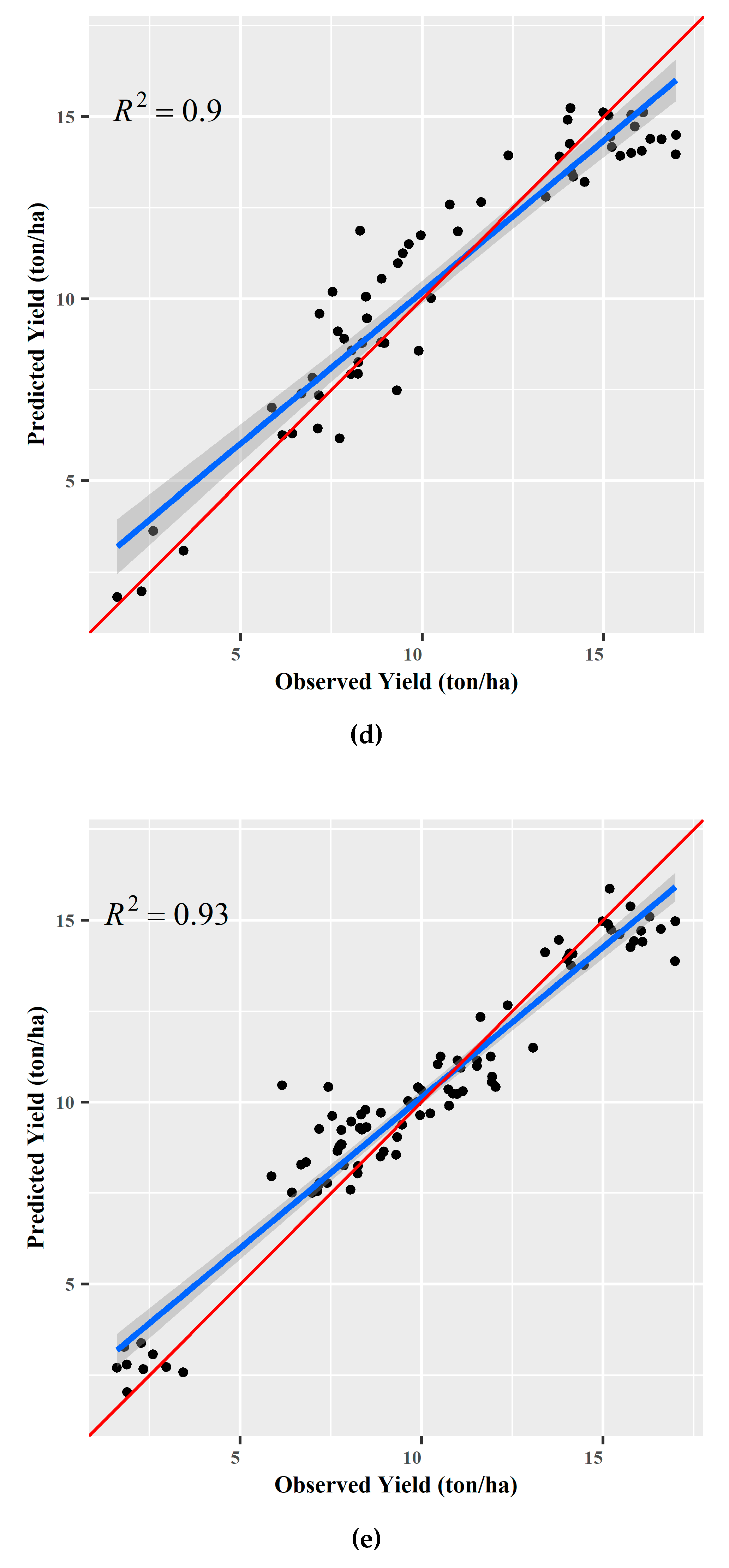
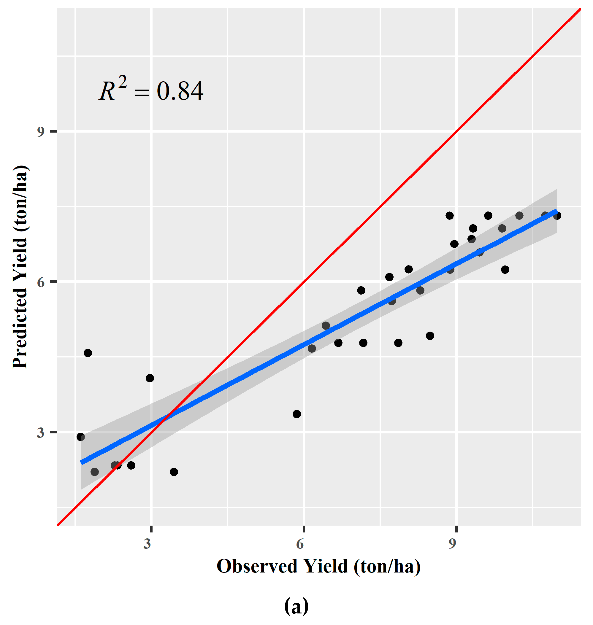
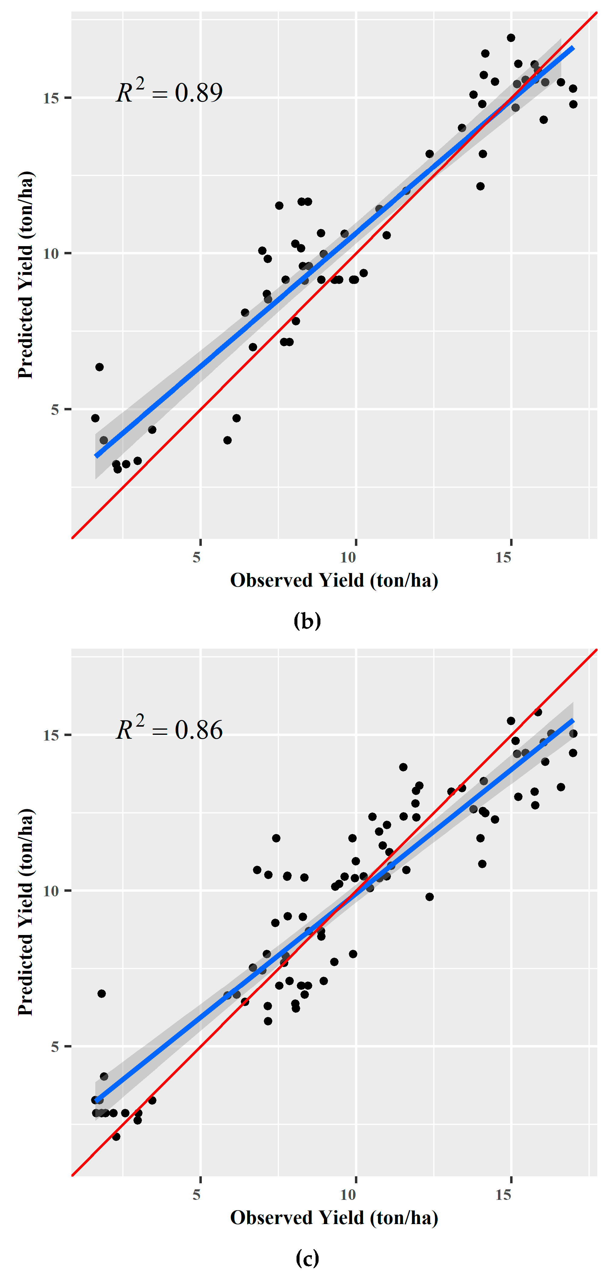
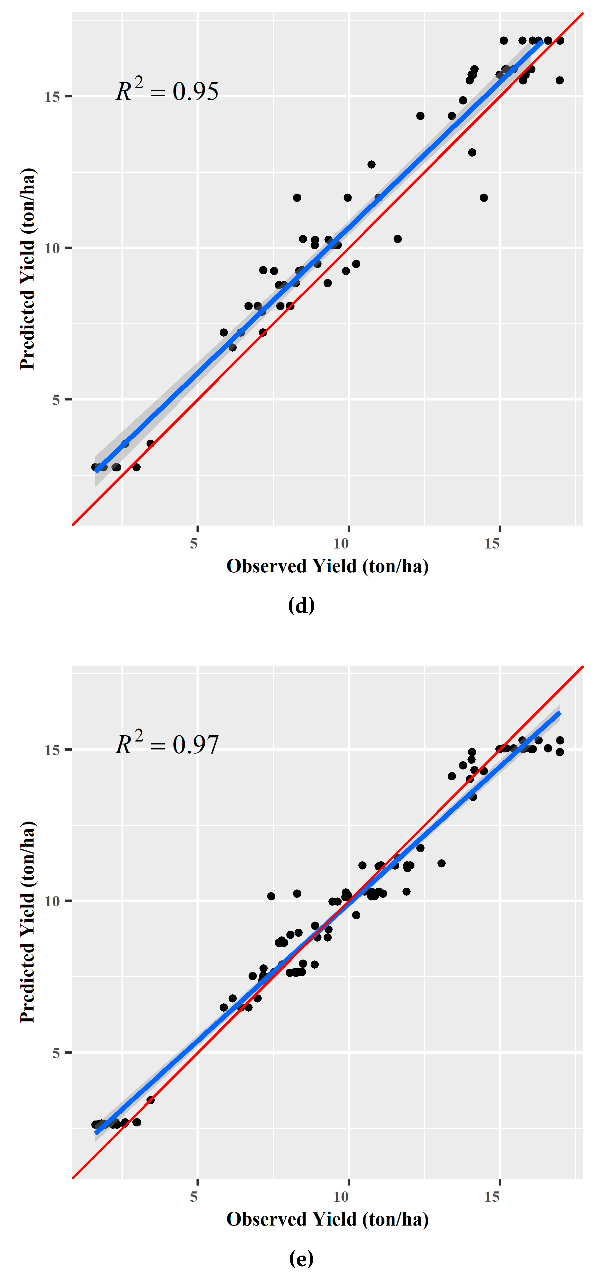
| Phenological Stage | Yield Prediction Models | R2-adj |
|---|---|---|
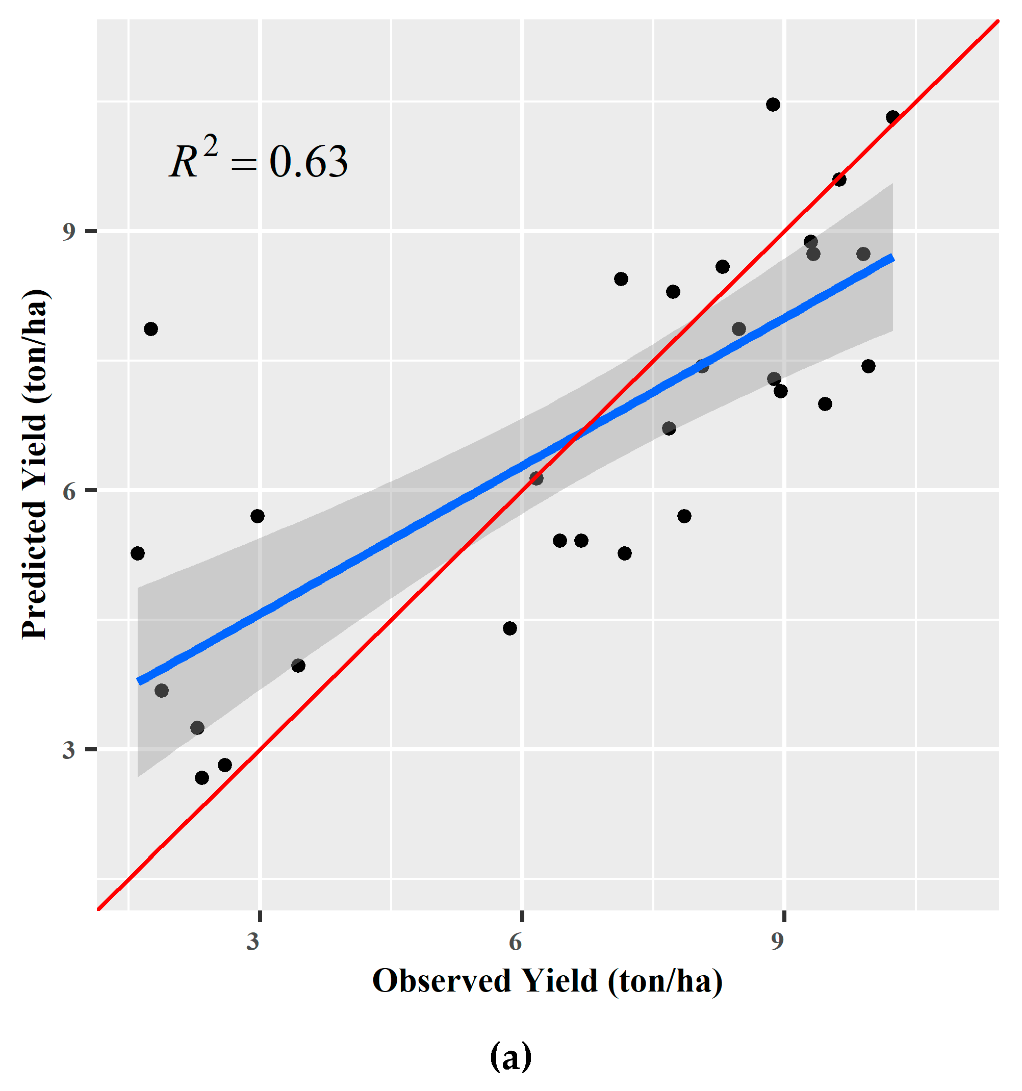
| V3 | Yield = − 23 + 144.4 OSAVI | 0.63 |
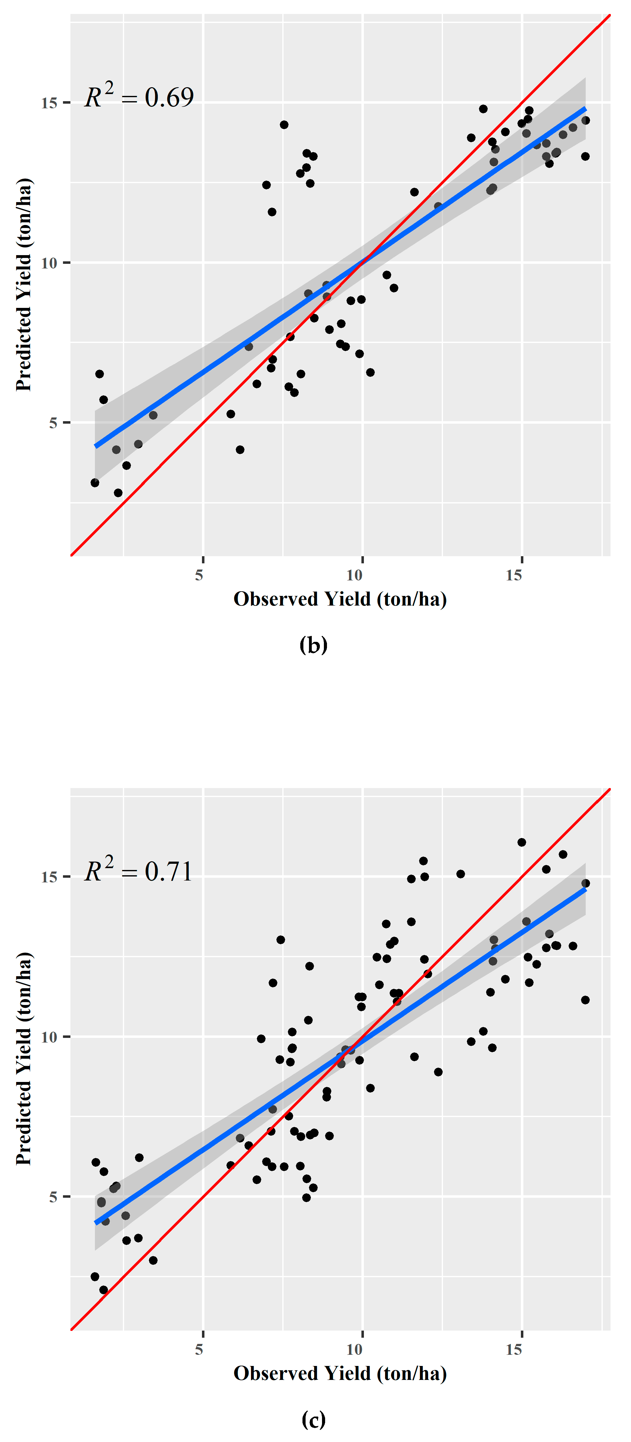
| V4-5 | Yield = − 13.36 + 45.48 SCCCI | 0.69 |
| V6-7 | Yield = − 161 + 590.3 GARI + 151.7 NDRE − 456.9 GNDVI | 0.70 |
| V10-11 | Yield = − 22.64 + 68.93 SCCCI − 19.13 SAVI | 0.90 |
| VT | Yield = − 10.96 + 26.07 SCCCI − 68.25 GLI + 13.25 VARIgreen | 0.93 |
© 2020 by the authors. Licensee MDPI, Basel, Switzerland. This article is an open access article distributed under the terms and conditions of the Creative Commons Attribution (CC BY) license (http://creativecommons.org/licenses/by/4.0/).
Share and Cite
Barzin, R.; Pathak, R.; Lotfi, H.; Varco, J.; Bora, G.C. Use of UAS Multispectral Imagery at Different Physiological Stages for Yield Prediction and Input Resource Optimization in Corn. Remote Sens. 2020, 12, 2392. https://doi.org/10.3390/rs12152392
Barzin R, Pathak R, Lotfi H, Varco J, Bora GC. Use of UAS Multispectral Imagery at Different Physiological Stages for Yield Prediction and Input Resource Optimization in Corn. Remote Sensing. 2020; 12(15):2392. https://doi.org/10.3390/rs12152392
Chicago/Turabian StyleBarzin, Razieh, Rohit Pathak, Hossein Lotfi, Jac Varco, and Ganesh C. Bora. 2020. "Use of UAS Multispectral Imagery at Different Physiological Stages for Yield Prediction and Input Resource Optimization in Corn" Remote Sensing 12, no. 15: 2392. https://doi.org/10.3390/rs12152392