Figure 1.
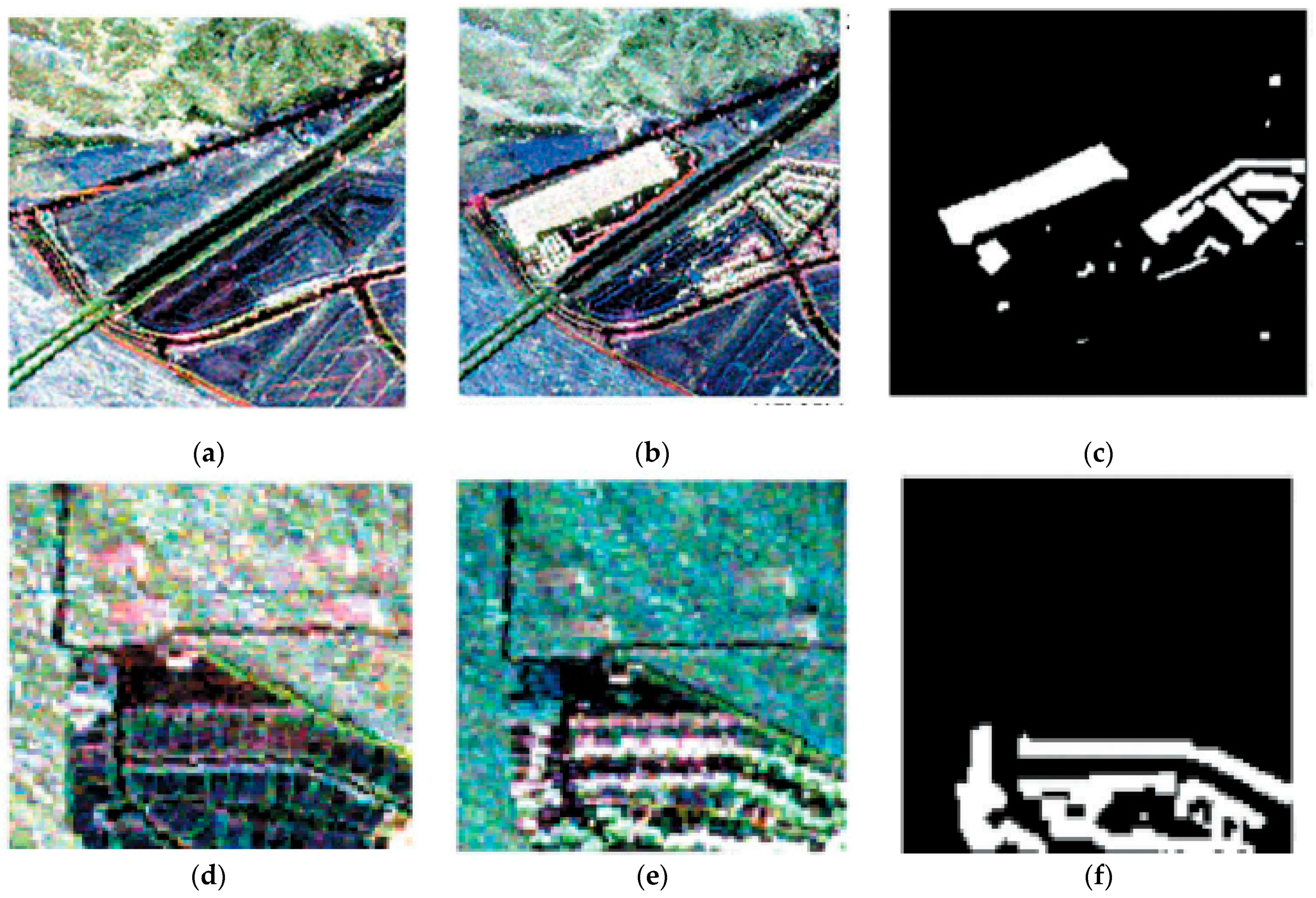
Multispectral datasets: (a) and (b) show the false-color composite of the multispectral images acquired over Abudhabi City, in United Arab Emirates (UAE) on 20 January 2016, and 28 March 2018, respectively, and (c) is the corresponding binary ground truth data which illustrates the change and no-change areas. (d) and (e) are the false-color composites of the multispectral images acquired over the Saclay area on 15 March 2016, and 29 October 2017, respectively, and (f) is the corresponding ground truth data, which white and black colors indicate the change and no-change areas, respectively.
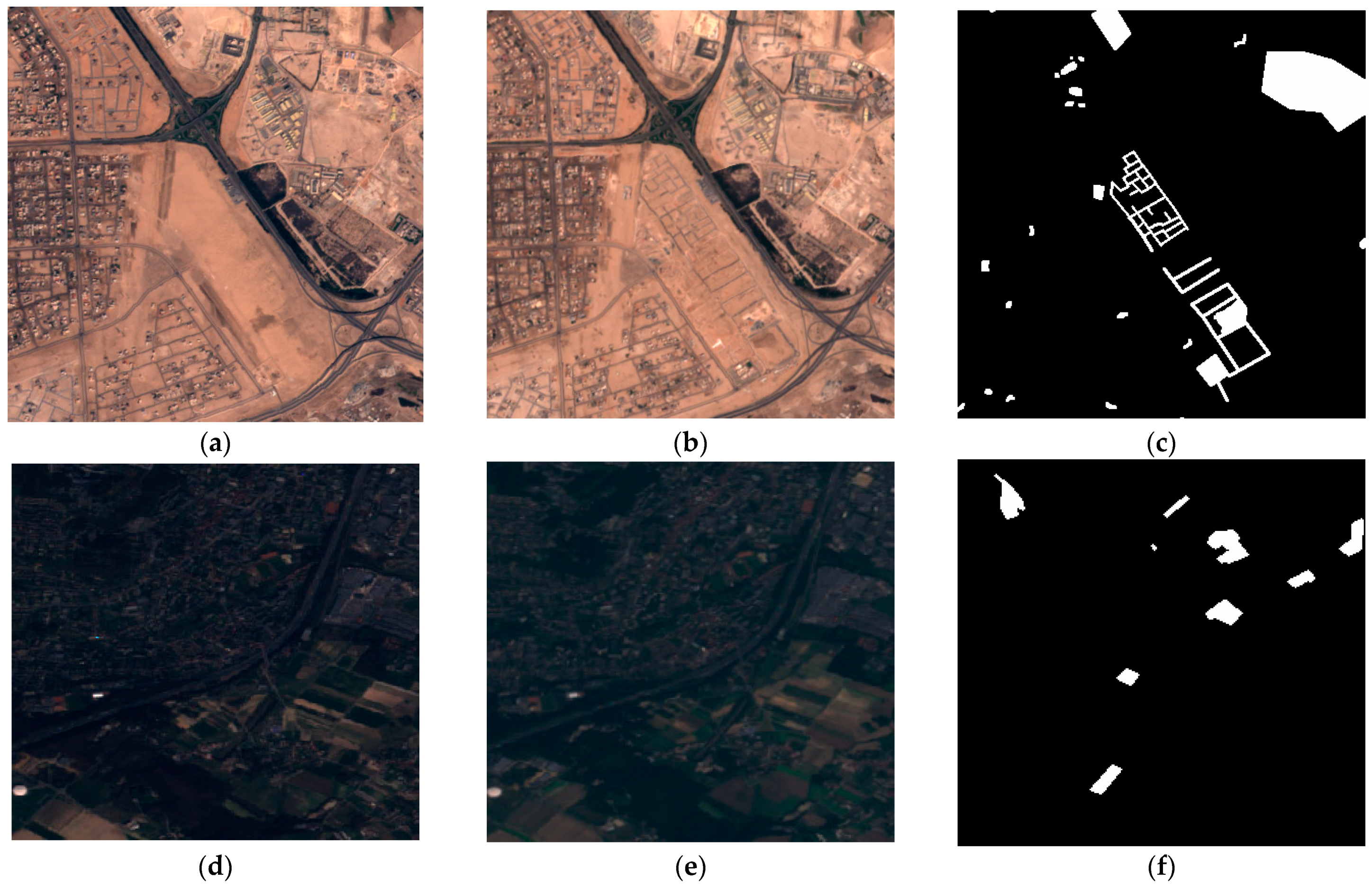
Figure 1.
Multispectral datasets: (a) and (b) show the false-color composite of the multispectral images acquired over Abudhabi City, in United Arab Emirates (UAE) on 20 January 2016, and 28 March 2018, respectively, and (c) is the corresponding binary ground truth data which illustrates the change and no-change areas. (d) and (e) are the false-color composites of the multispectral images acquired over the Saclay area on 15 March 2016, and 29 October 2017, respectively, and (f) is the corresponding ground truth data, which white and black colors indicate the change and no-change areas, respectively.
Figure 2.
Hyperspectral datasets: (a) and (b) are a false-color composite of the Hyperspectral-River images acquired over a river in Jiangsu province, China on 3 May 2013, and 31 December 2013, respectively, and (c) is the corresponding binary ground truth data, which white and black colors indicate the change and no-change areas, respectively. (d) and (e) are a false-color composite of the Hyperspectral-Farmland images acquired over farmland in the USA on 1 May 2004, and 8 May 2007, respectively, and (f) is the corresponding ground truth data in binary format, which white and black colors indicate the change and no-change areas, respectively.
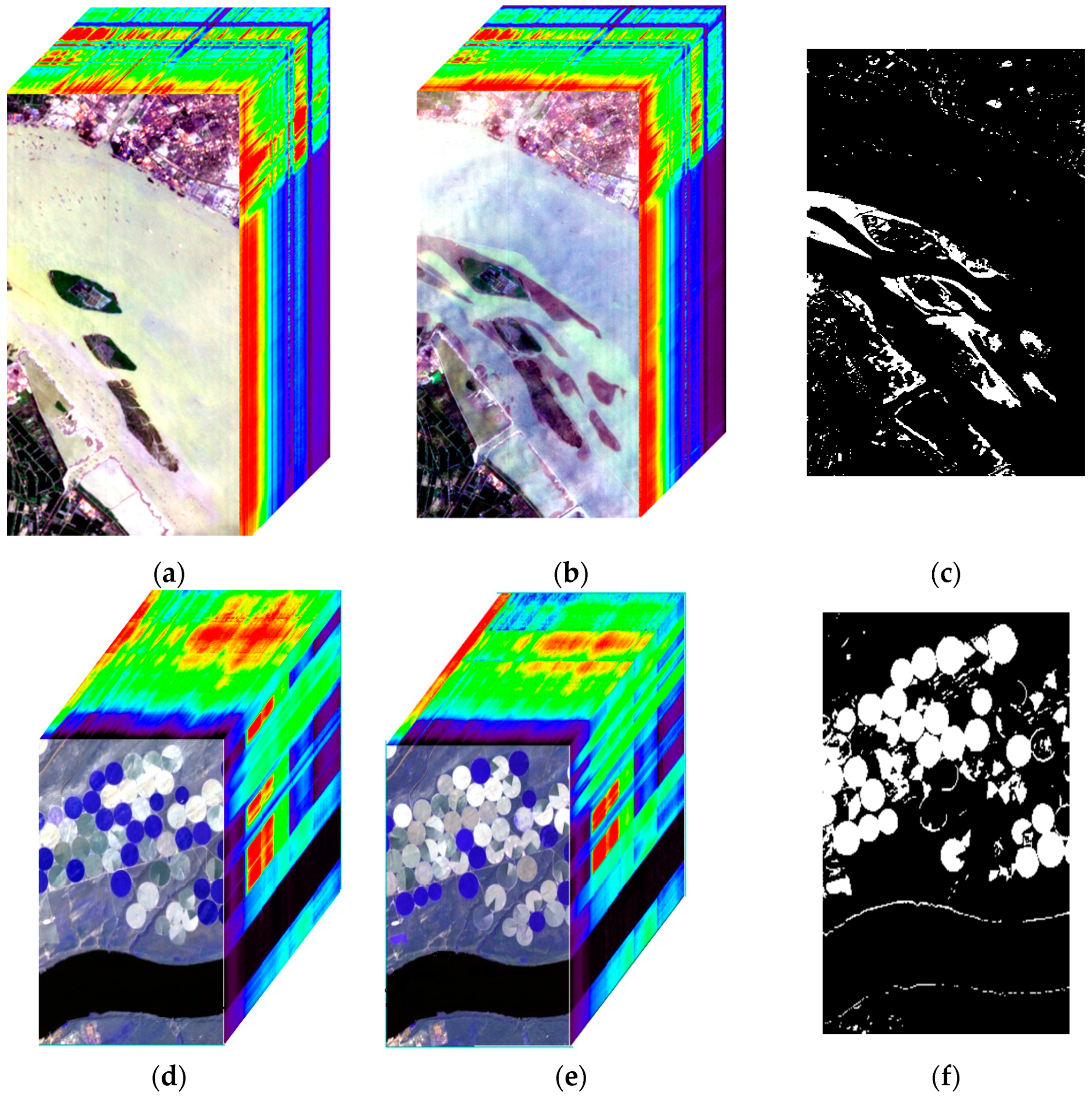
Figure 3.
PolSAR dataset: (a) and (b) are the RGB composites generated from the Pauli decomposition (Red: |HH − VV|; Green: 2|HV|; Blue: |HH + VV|) for the PolSAR-San Francisco1 datasets, and (c) shows the corresponding binary ground truth data, which white and black colors indicate the change and no-change areas, respectively. (d) and (e) are Pauli RGB composite of the PolSAR-San Francisco2 images, and (f) shows the corresponding ground truth data in binary format, which white and black colors indicate the change and no-change areas, respectively. Note that (a) and (d) were acquired on 18 September 2009, and (b) and (e) were captured on 11 May 2015.
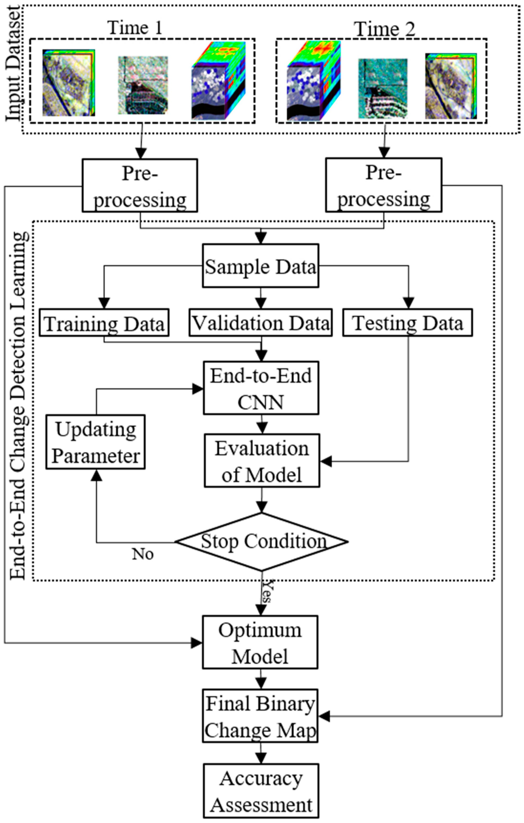
Figure 4.
General flowchart of the proposed supervised binary change detection (CD) method.
Figure 4.
General flowchart of the proposed supervised binary change detection (CD) method.
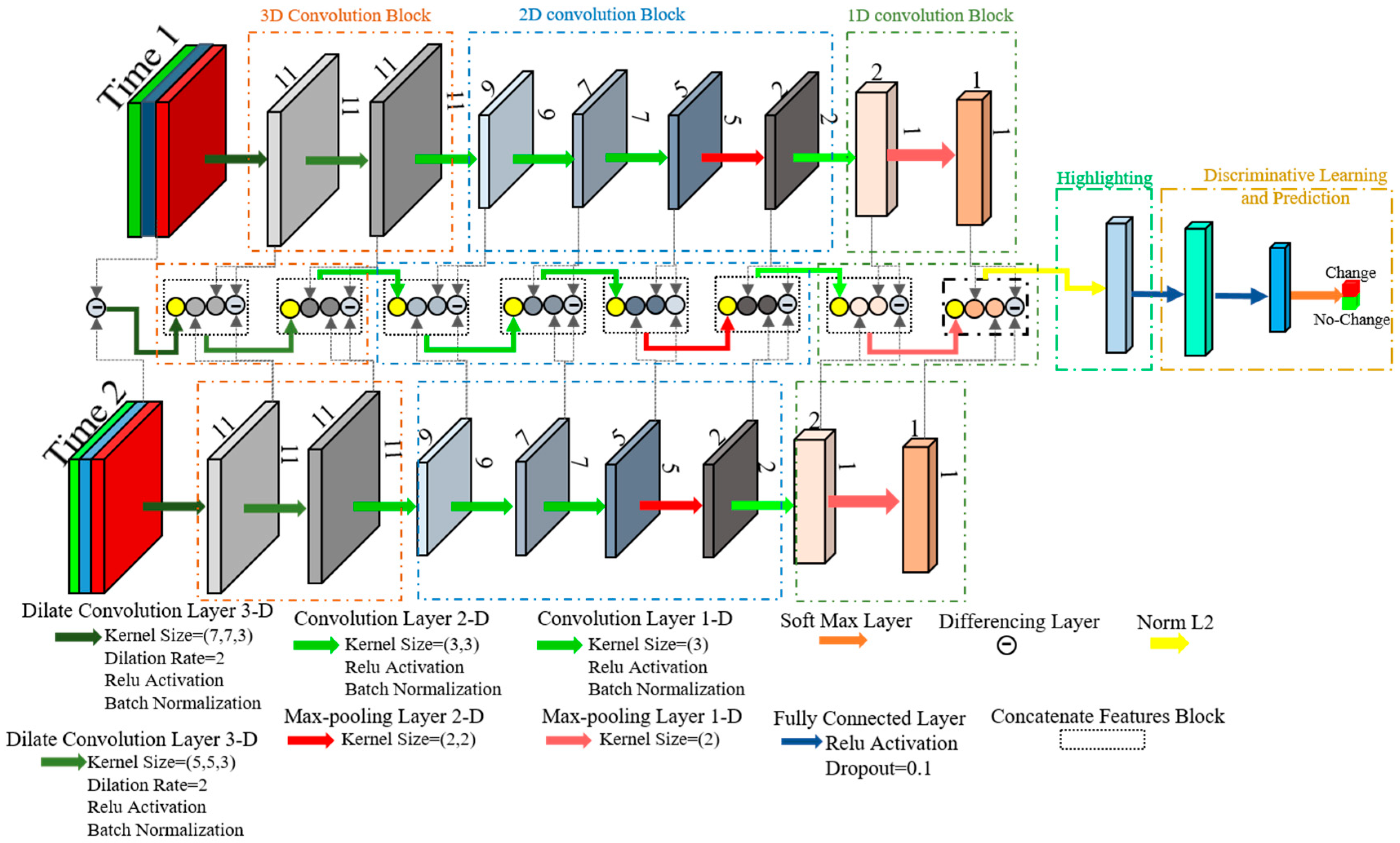
Figure 5.
The proposed End-to-End convolutional neural network (CNN) architecture for CD of remote sensing datasets.
Figure 5.
The proposed End-to-End convolutional neural network (CNN) architecture for CD of remote sensing datasets.
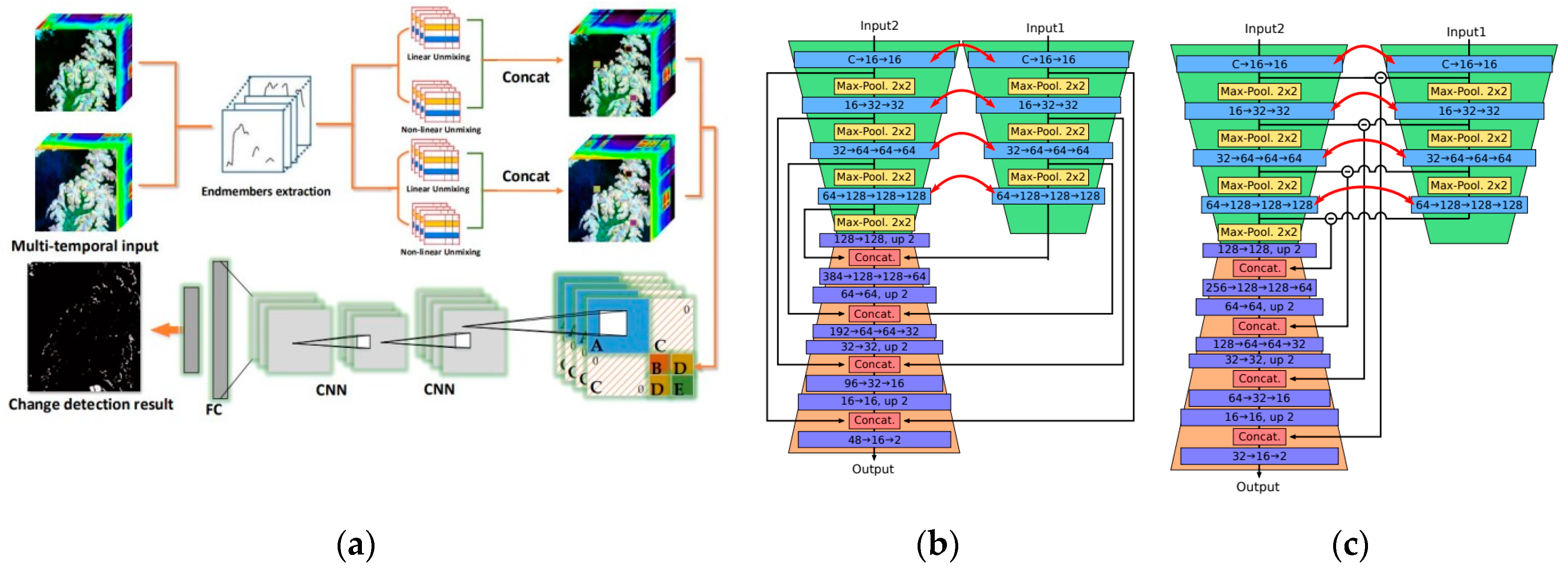
Figure 6.
Overview of the three state-of-the-art CD frameworks based on deep learning. (
a) General End-to-end Two-dimensional CNN Framework (GETNET) [
29], (
b) Siamese-concatenate network [
44], and (
c) Siamese-differencing network [
44].
Figure 6.
Overview of the three state-of-the-art CD frameworks based on deep learning. (
a) General End-to-end Two-dimensional CNN Framework (GETNET) [
29], (
b) Siamese-concatenate network [
44], and (
c) Siamese-differencing network [
44].
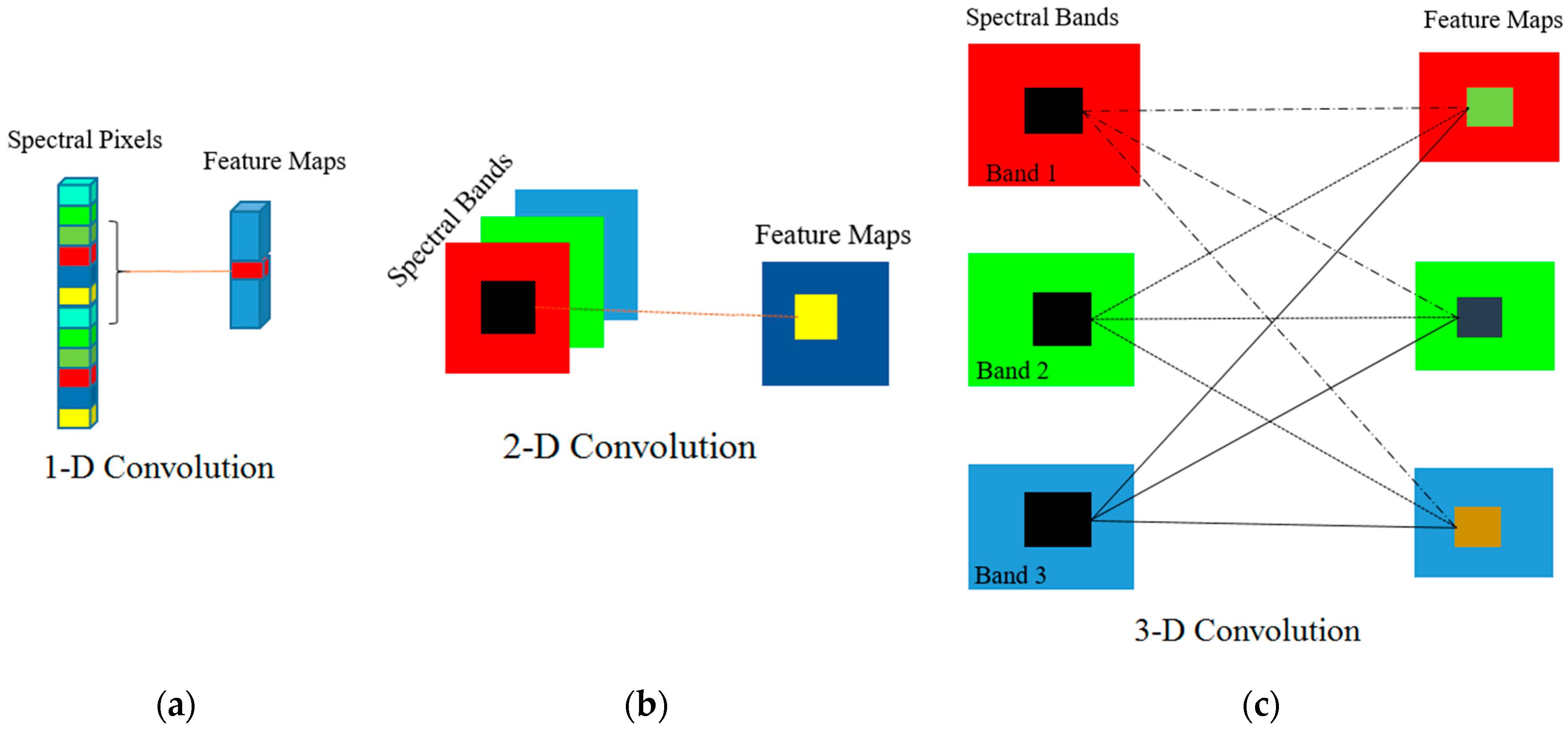
Figure 7.
Comparison of (a) 1-D, (b) 2-D, and (c) 3-D convolution layers.
Figure 7.
Comparison of (a) 1-D, (b) 2-D, and (c) 3-D convolution layers.
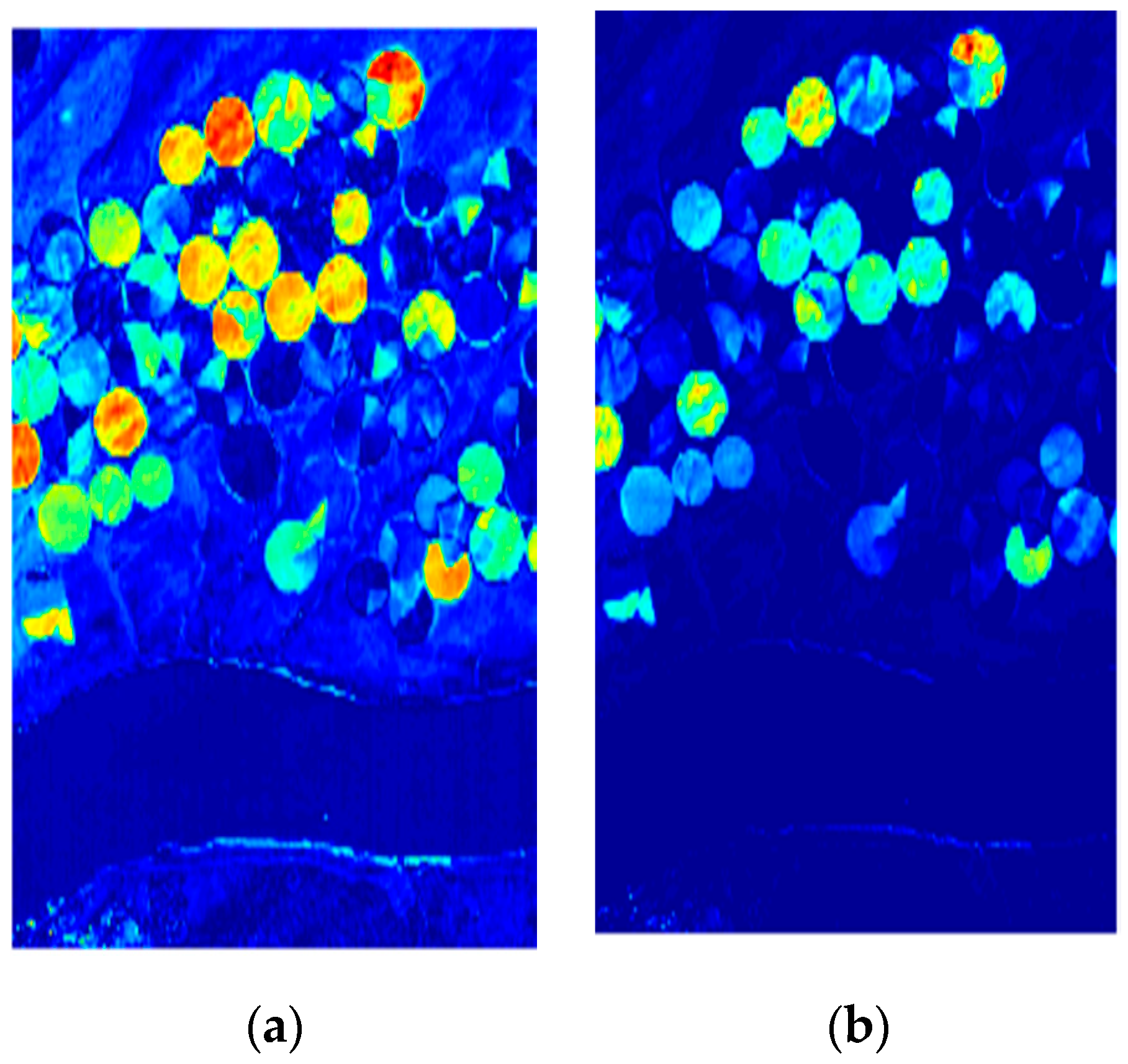
Figure 8.
The difference between (a) simple differencing and (b) norm l2 in discriminating change and no-change areas for Hyperspectral-Farmland datasets.
Figure 8.
The difference between (a) simple differencing and (b) norm l2 in discriminating change and no-change areas for Hyperspectral-Farmland datasets.
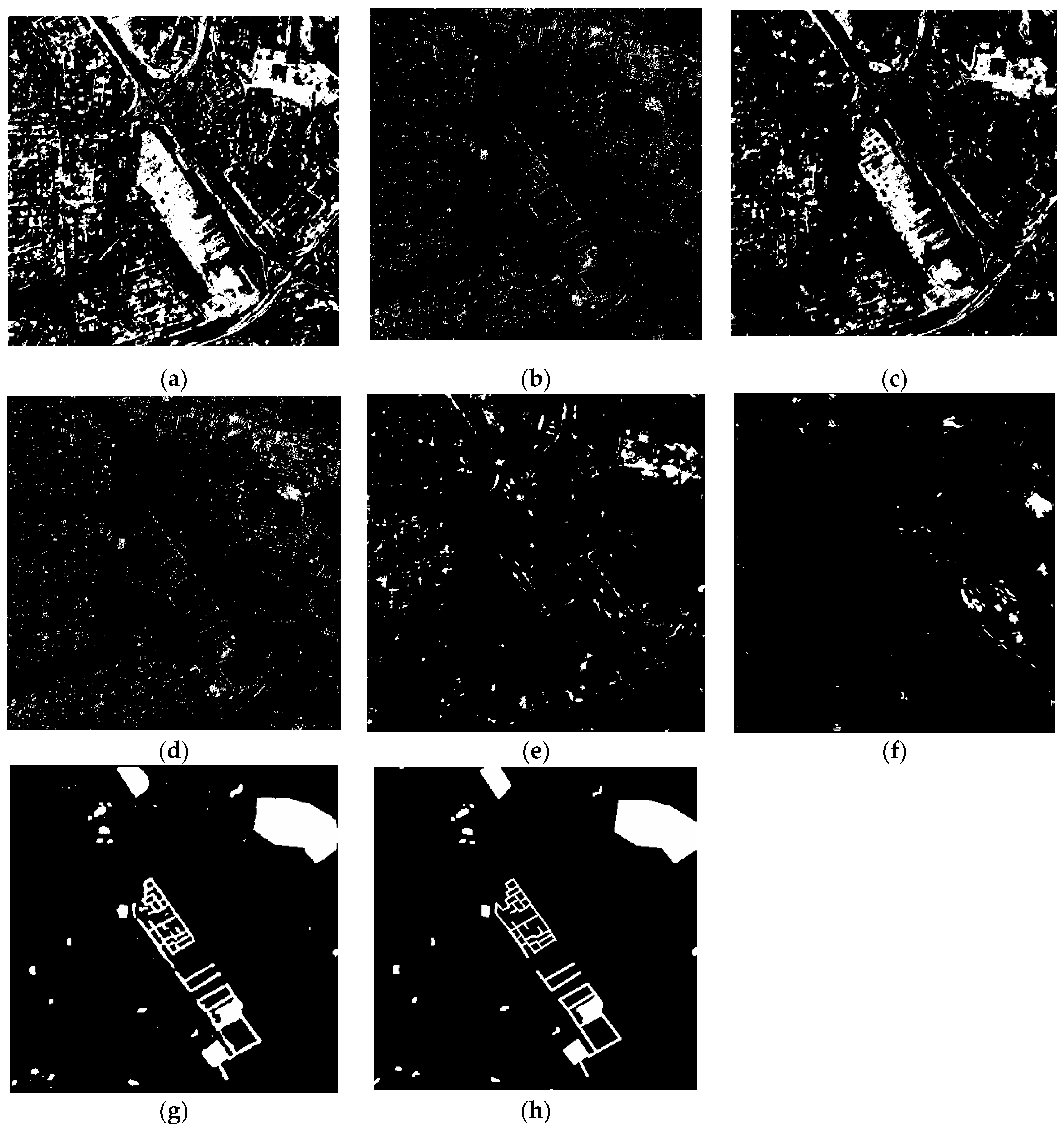
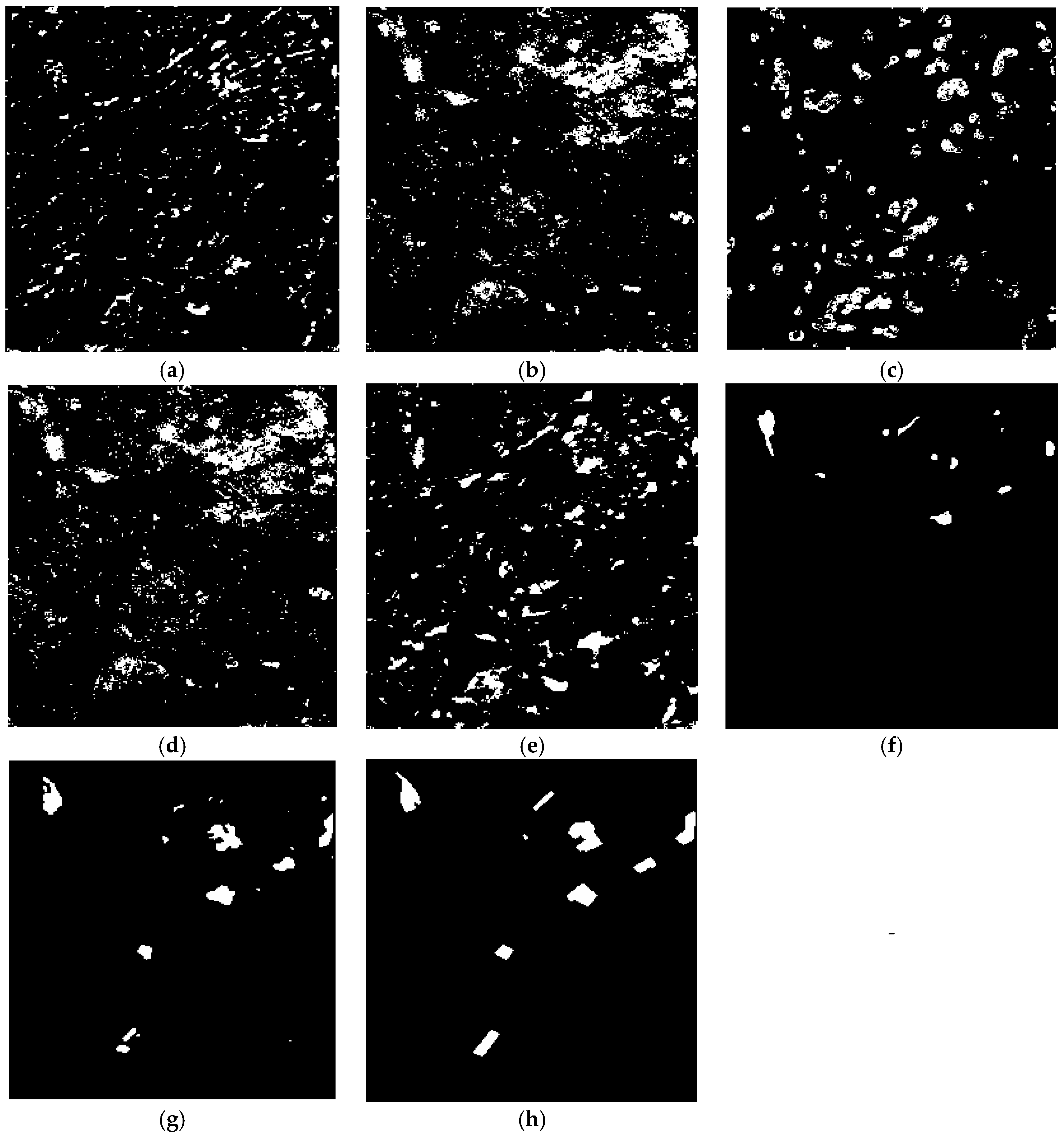
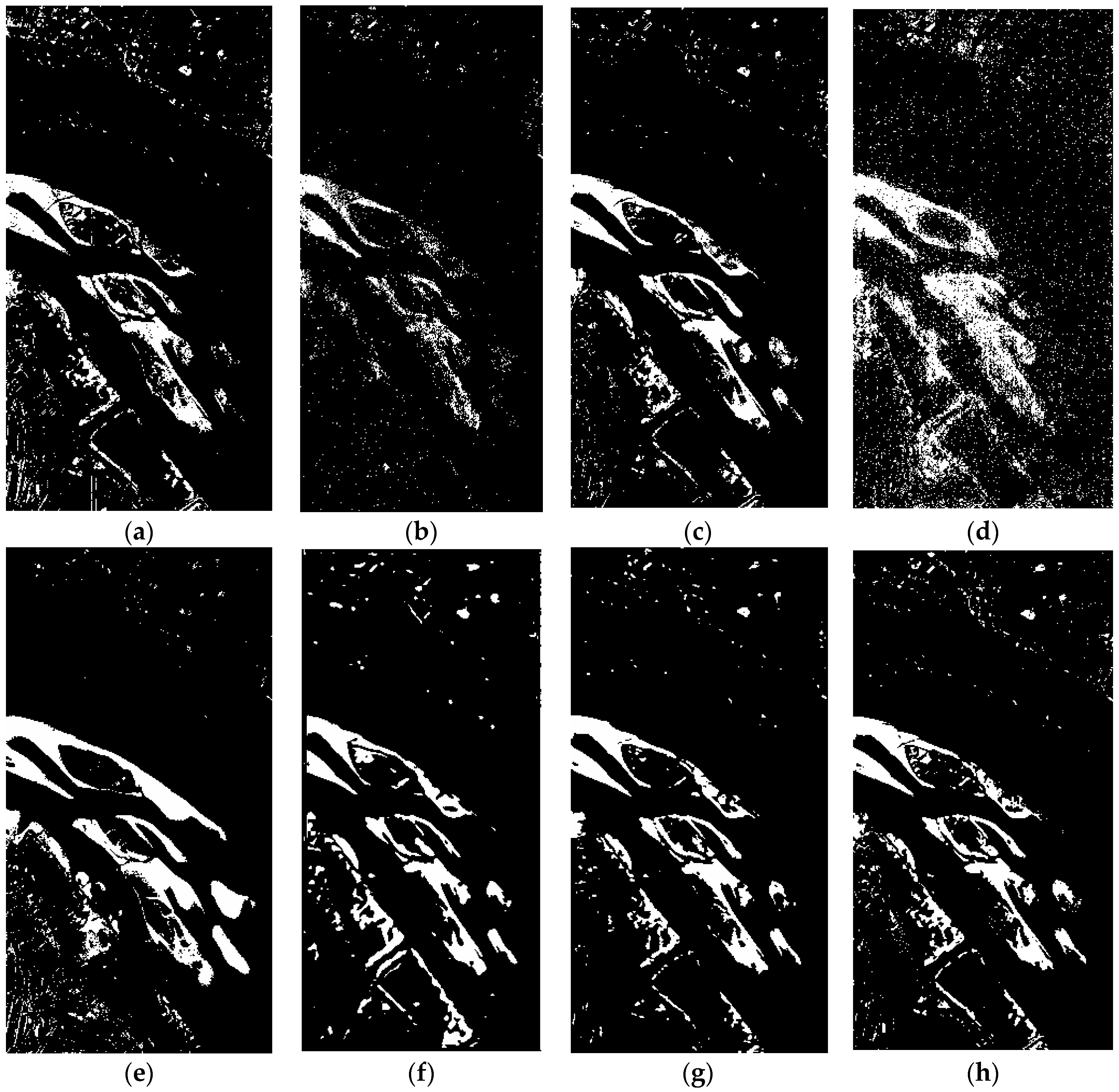
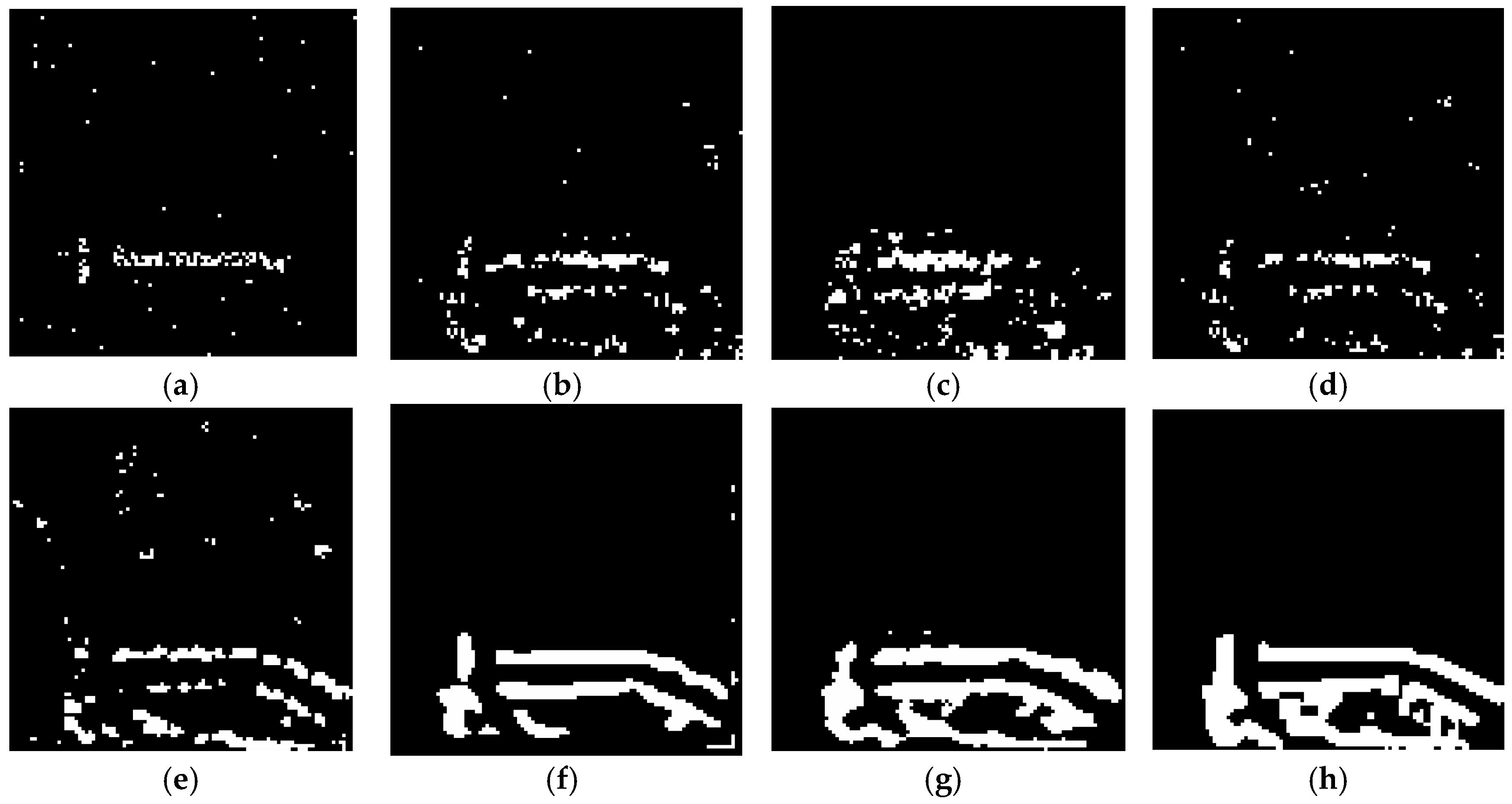
Figure 9.
The change detection maps produced by different CD methods for the Multispectral-Abudhabi dataset. (a) CVA-SVM, (b) MAD-SVM, (c) PCA-SVM, (d) IR-MAD -SVM, (e) SFA-SVM, (f) 3D-CNN, (g) Proposed Method, and (h) Ground Truth. White and black colors indicate the change and no-change areas, respectively.
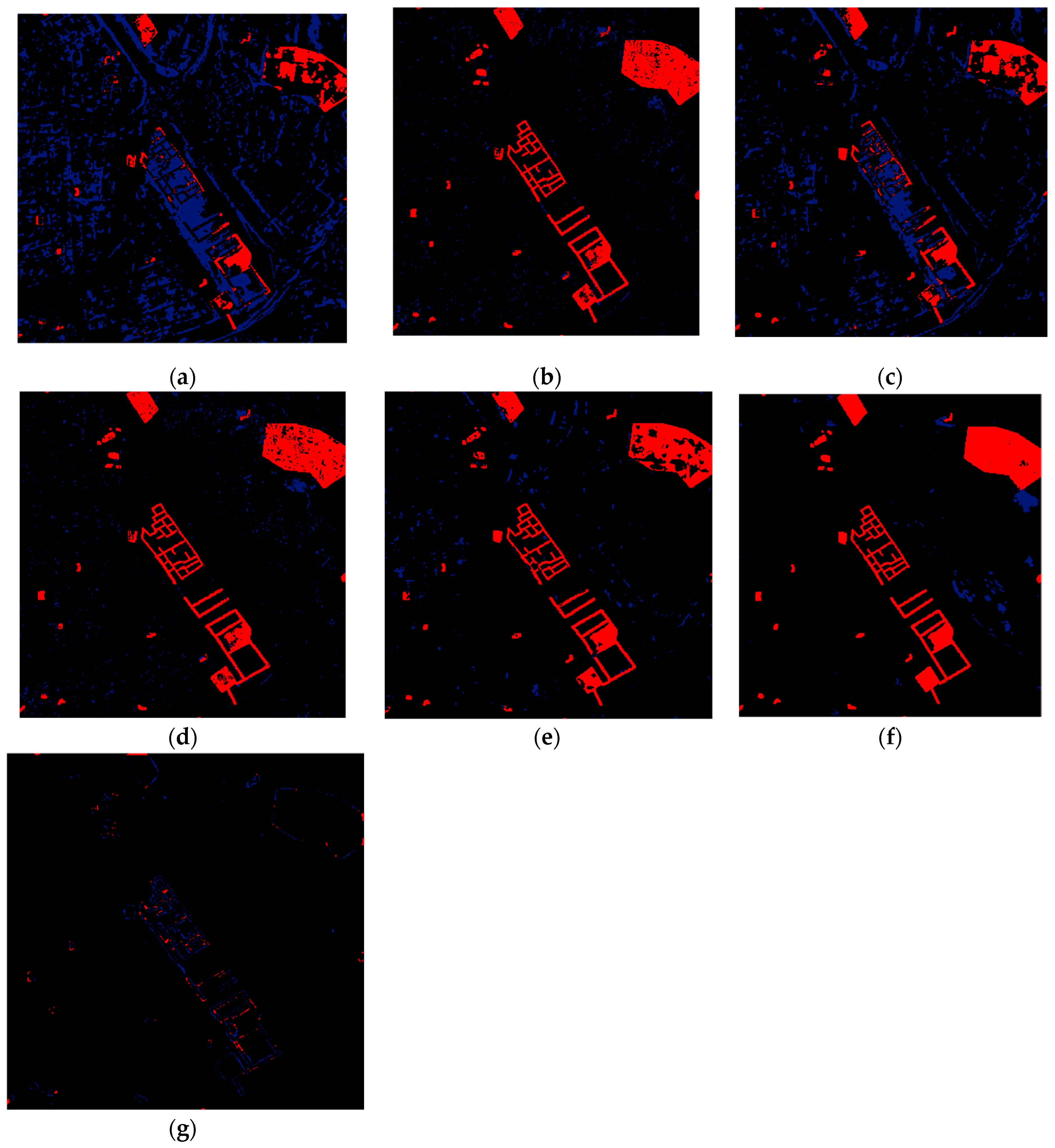
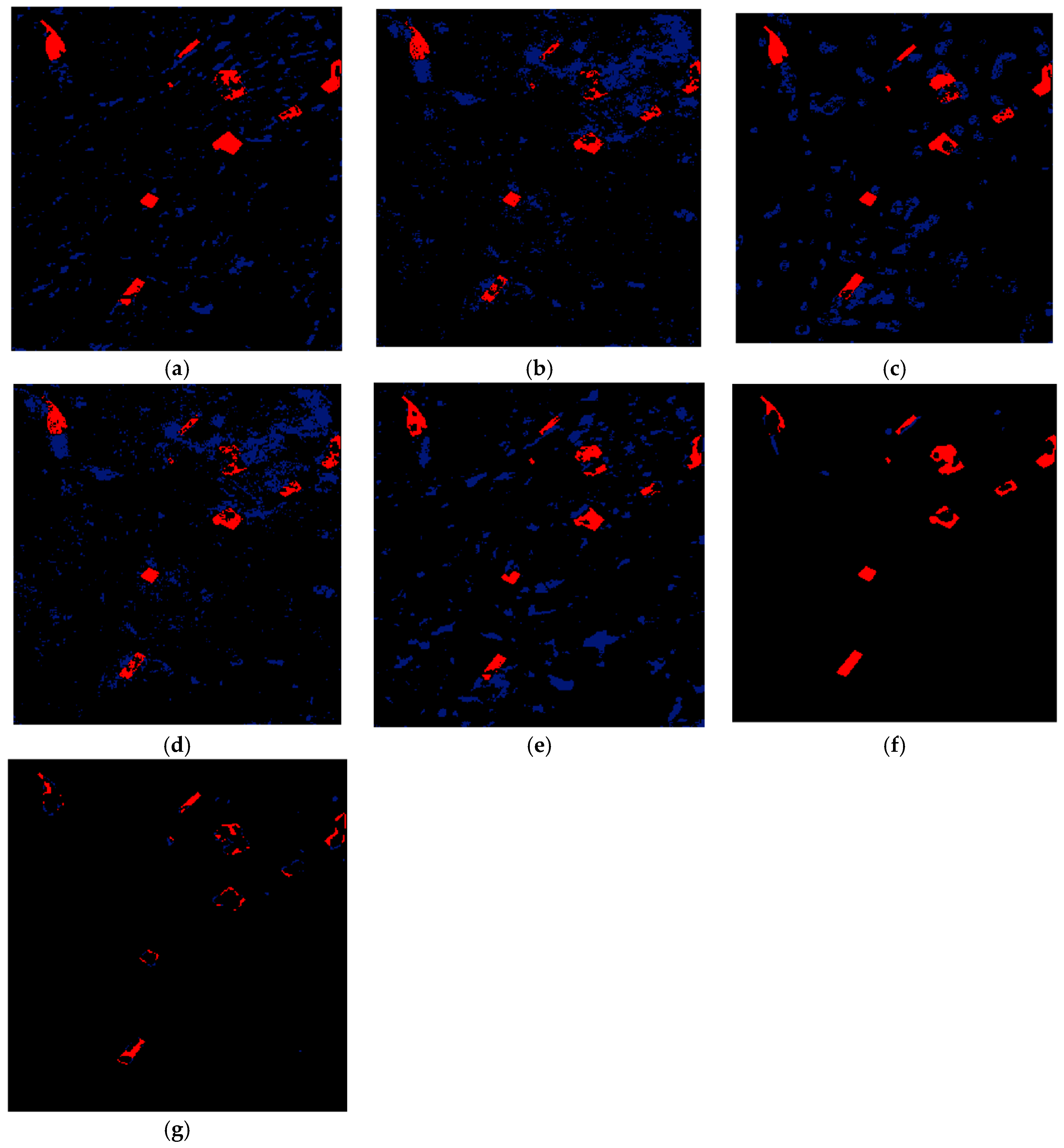
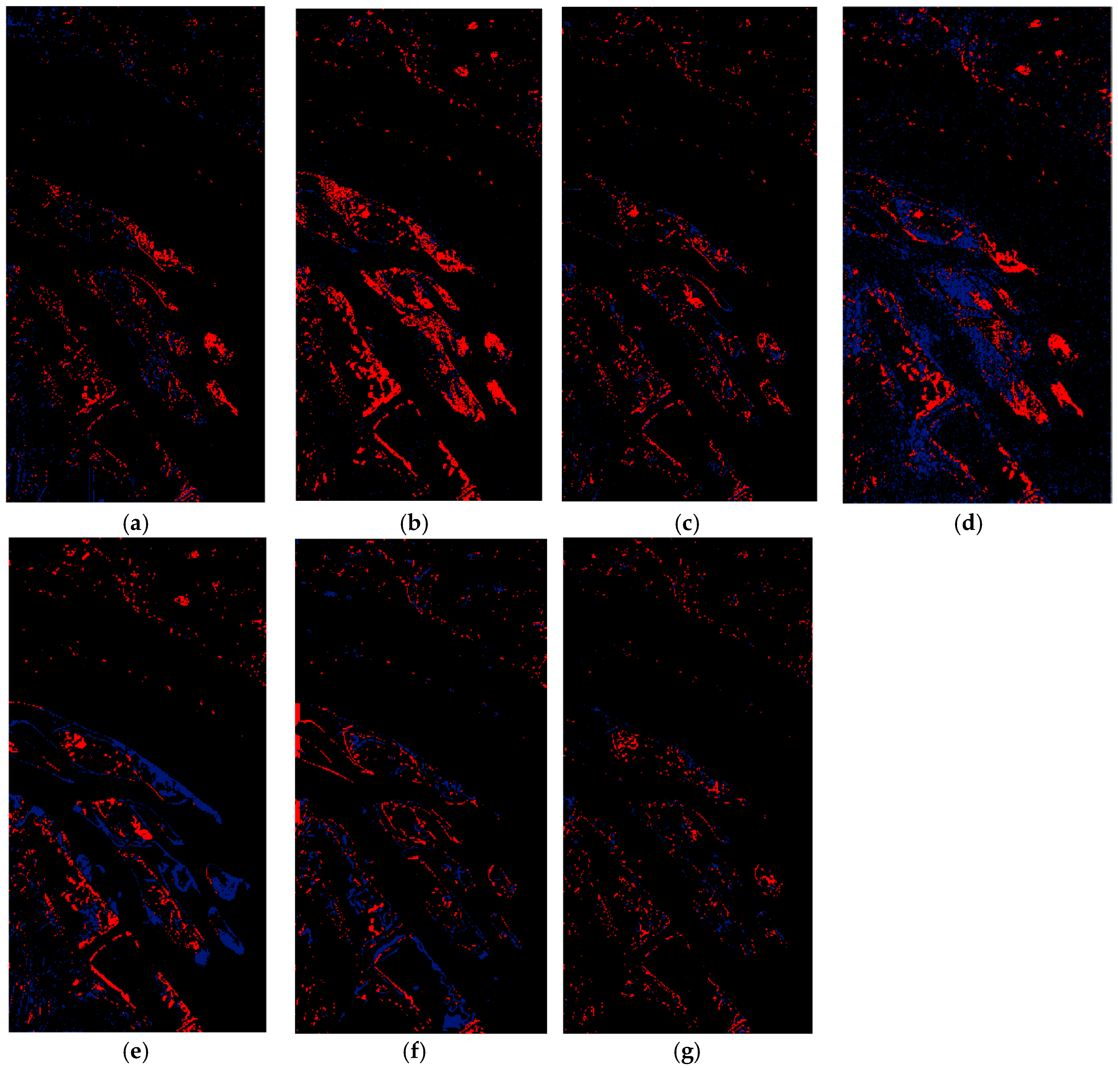
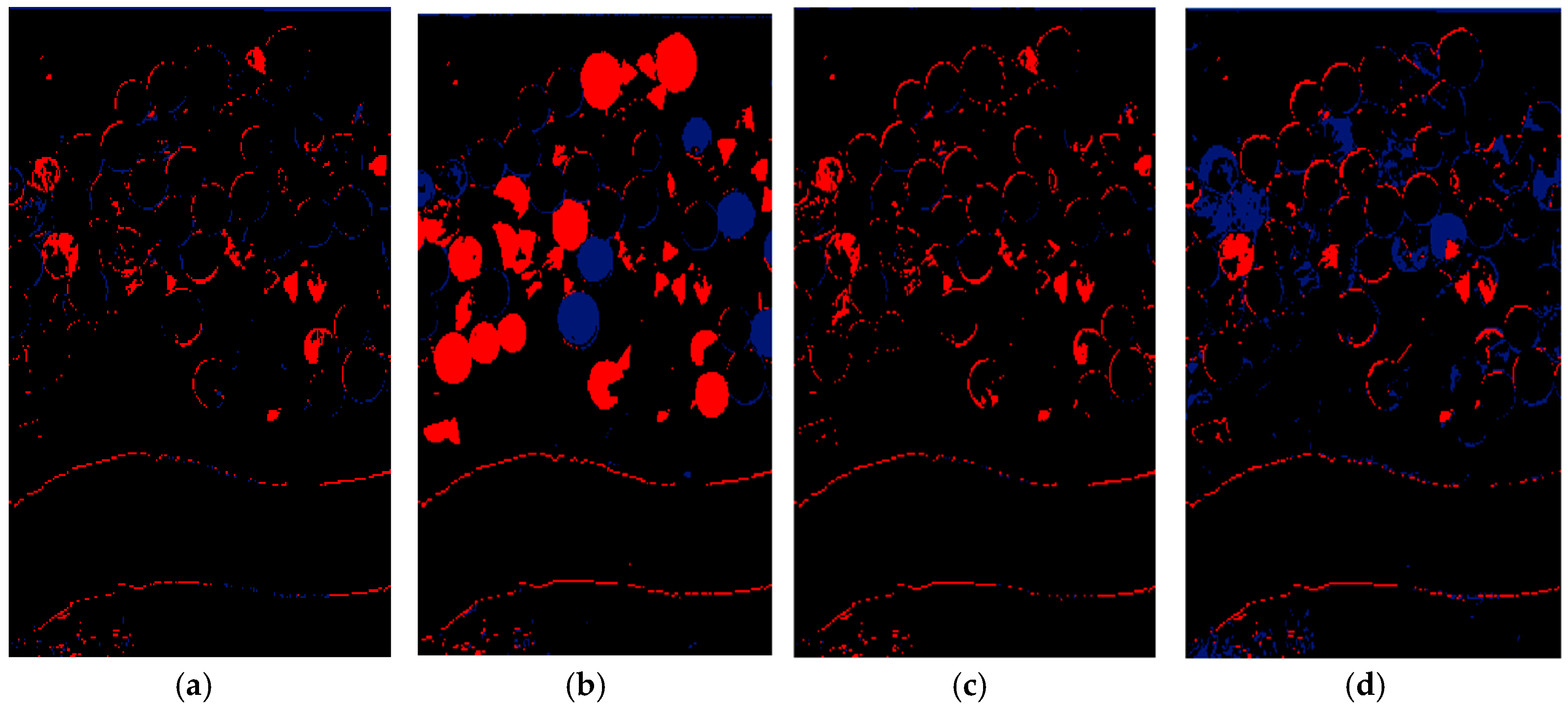
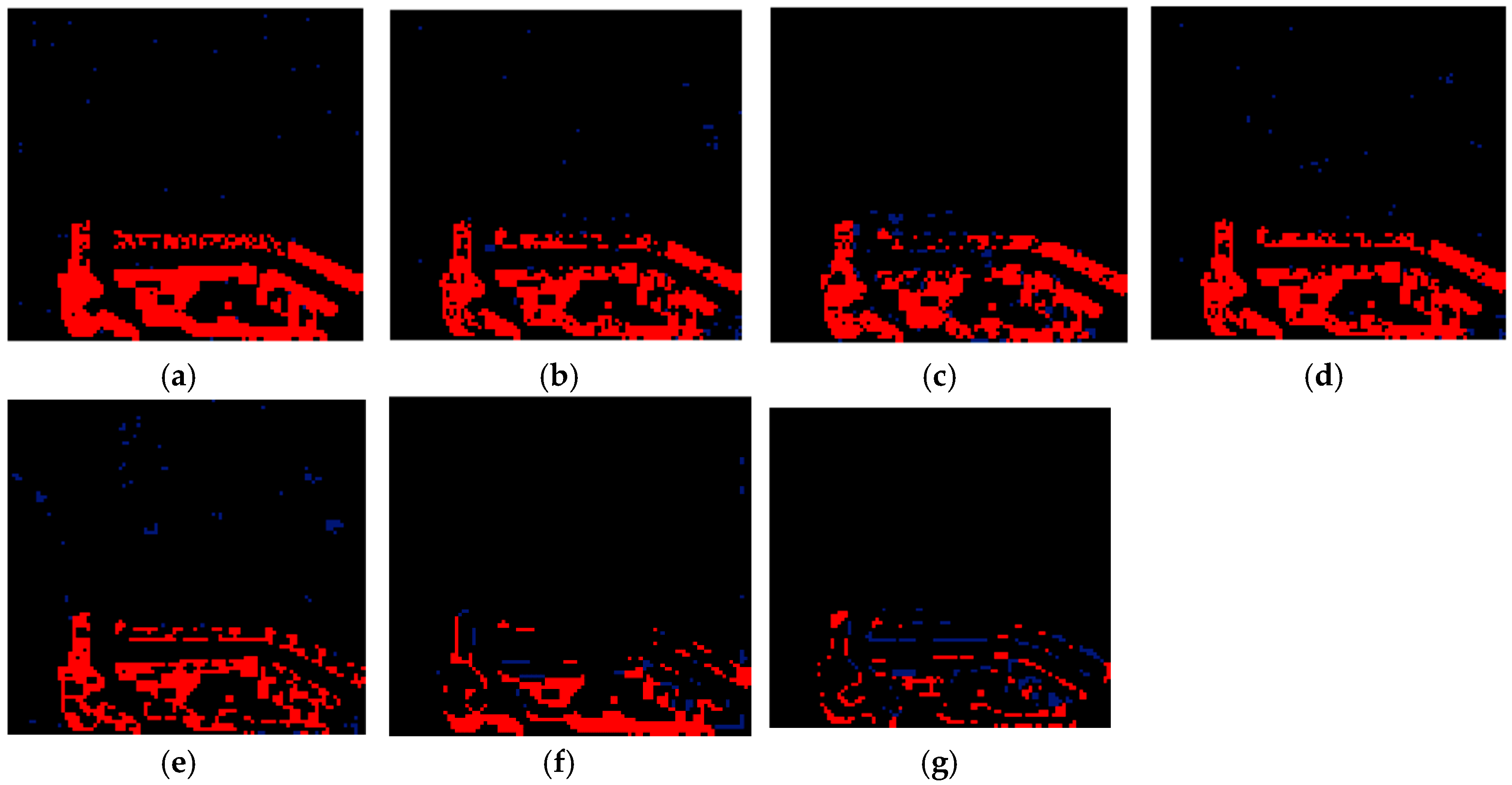
Figure 10.
The errors in change detection using different methods for the Multispectral-Abudhabi dataset. (a) CVA-SVM, (b) MAD-SVM, (c) PCA-SVM, (d) IR-MAD -SVM, (e) SFA-SVM, (f) 3D-CNN, and (g) Proposed Method. Black, red, and blue colors indicate TP and TN, FN, and FP respectively.
Figure 10.
The errors in change detection using different methods for the Multispectral-Abudhabi dataset. (a) CVA-SVM, (b) MAD-SVM, (c) PCA-SVM, (d) IR-MAD -SVM, (e) SFA-SVM, (f) 3D-CNN, and (g) Proposed Method. Black, red, and blue colors indicate TP and TN, FN, and FP respectively.
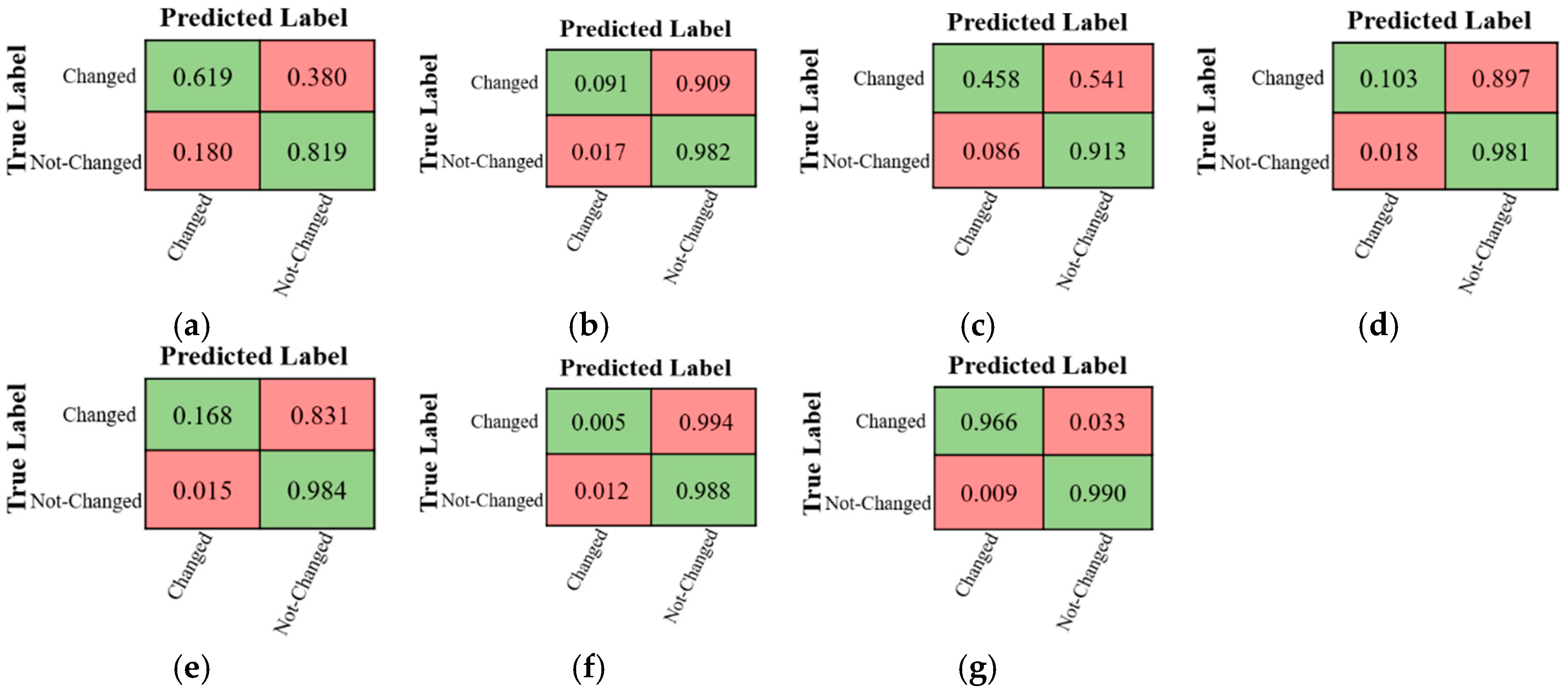
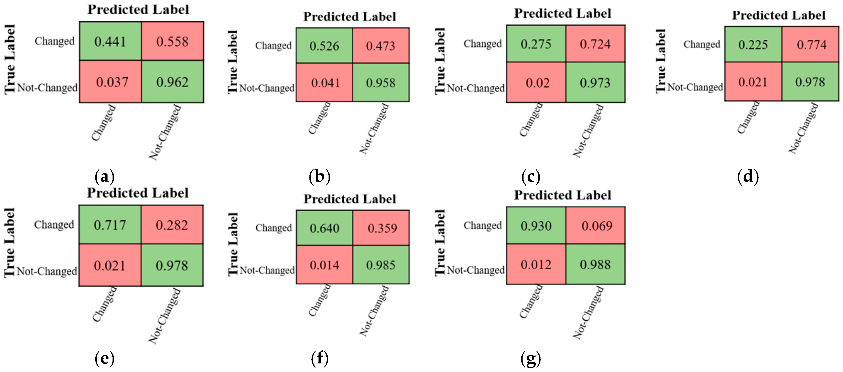
Figure 11.
The confusion matrices of different CD methods for the Multispectral-Abudhabi dataset. (a) CVA-SVM, (b) MAD-SVM, (c) PCA-SVM, (d) IR-MAD -SVM, (e) SFA-SVM, (f) 3D-CNN, and (g) Proposed Method.
Figure 11.
The confusion matrices of different CD methods for the Multispectral-Abudhabi dataset. (a) CVA-SVM, (b) MAD-SVM, (c) PCA-SVM, (d) IR-MAD -SVM, (e) SFA-SVM, (f) 3D-CNN, and (g) Proposed Method.
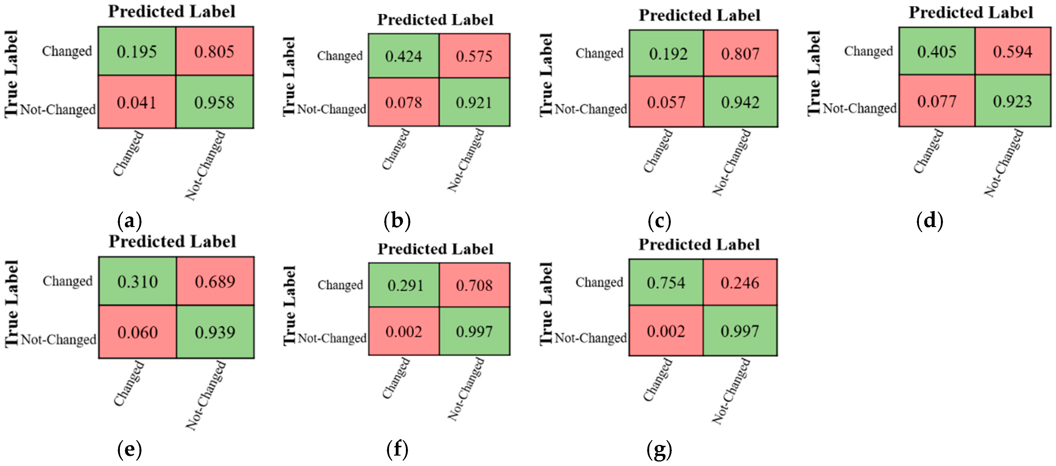
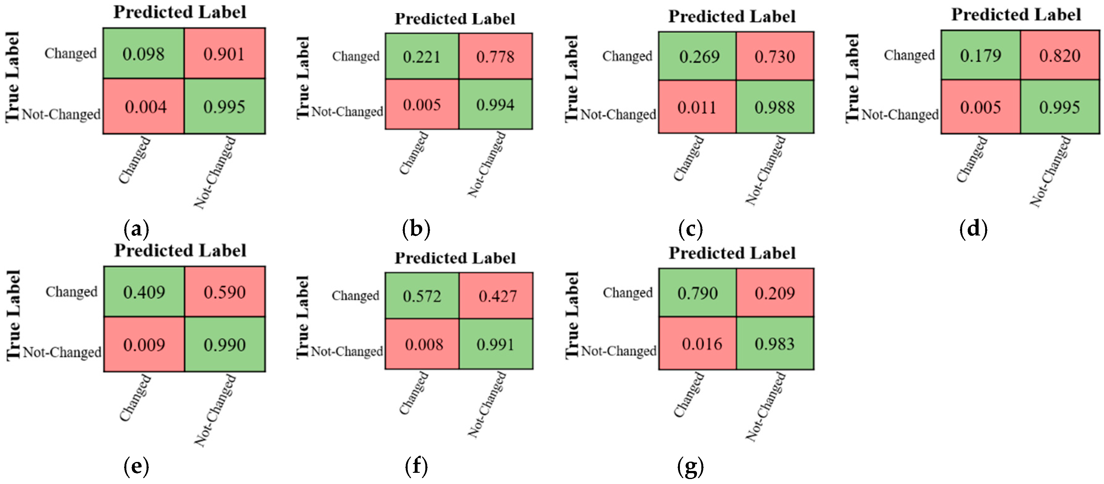
Figure 12.
The change detection maps produced by different methods for the Multispectral-Saclay dataset. (a) CVA-SVM, (b) MAD-SVM, (c) PCA-SVM, (d) IR-MAD -SVM, (e) SFA-SVM, (f) 3D-CNN, (g) Proposed Method, and (h) Ground Truth. White and black colors indicate the change and no-change areas, respectively.
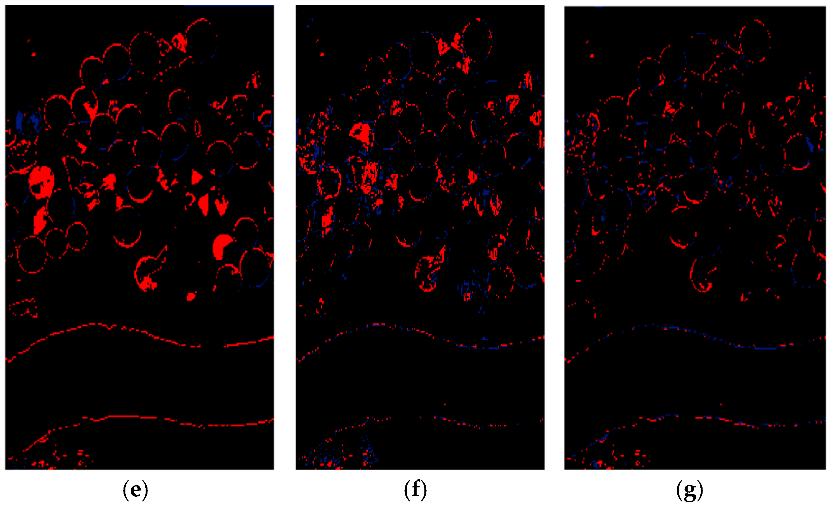
Figure 13.
The change detection errors of different methods for the Multispectral-Saclay dataset. (a) CVA-SVM, (b) MAD-SVM, (c) PCA-SVM, (d) IR-MAD -SVM, (e) SFA-SVM, (f) 3D-CNN, and (g) Proposed Method. Black, red, and blue colors indicate TP and TN, FN, and FP pixels, respectively.
Figure 13.
The change detection errors of different methods for the Multispectral-Saclay dataset. (a) CVA-SVM, (b) MAD-SVM, (c) PCA-SVM, (d) IR-MAD -SVM, (e) SFA-SVM, (f) 3D-CNN, and (g) Proposed Method. Black, red, and blue colors indicate TP and TN, FN, and FP pixels, respectively.
Figure 14.
The confusion matrices of different CD methods for the Multispectral-Saclay dataset. (a) CVA-SVM, (b) MAD-SVM, (c) PCA-SVM, (d) IR-MAD -SVM, (e) SFA-SVM, (f) 3D-CNN, and (g) Proposed Method.
Figure 14.
The confusion matrices of different CD methods for the Multispectral-Saclay dataset. (a) CVA-SVM, (b) MAD-SVM, (c) PCA-SVM, (d) IR-MAD -SVM, (e) SFA-SVM, (f) 3D-CNN, and (g) Proposed Method.
Figure 15.
The change detection maps obtained by different methods for the Hyperspectral-River dataset. (a) CVA-SVM, (b) MAD-SVM, (c) PCA-SVM, (d) IR-MAD -SVM, (e) SFA-SVM, (f) 3D-CNN, (g) Proposed Method, and (h) Ground Truth. White and black colors indicate the change and no-change areas, respectively.
Figure 16.
The change detection errors of different methods for the Hyperspectral-River dataset. (a) CVA-SVM, (b) MAD-SVM, (c) PCA-SVM, (d) IR-MAD -SVM, (e) SFA-SVM, (f) 3D-CNN, and (g) Proposed Method. Black, red, and blue colors indicate TP and TN, FN, and FP pixels respectively.
Figure 16.
The change detection errors of different methods for the Hyperspectral-River dataset. (a) CVA-SVM, (b) MAD-SVM, (c) PCA-SVM, (d) IR-MAD -SVM, (e) SFA-SVM, (f) 3D-CNN, and (g) Proposed Method. Black, red, and blue colors indicate TP and TN, FN, and FP pixels respectively.
Figure 17.
The confusion matrices of different CD methods for the Hyperspectral-River dataset. (a) CVA-SVM, (b) MAD-SVM, (c) PCA-SVM, (d) IR-MAD -SVM, (e) SFA-SVM, (f) 3D-CNN, and (g) Proposed Method.
Figure 17.
The confusion matrices of different CD methods for the Hyperspectral-River dataset. (a) CVA-SVM, (b) MAD-SVM, (c) PCA-SVM, (d) IR-MAD -SVM, (e) SFA-SVM, (f) 3D-CNN, and (g) Proposed Method.
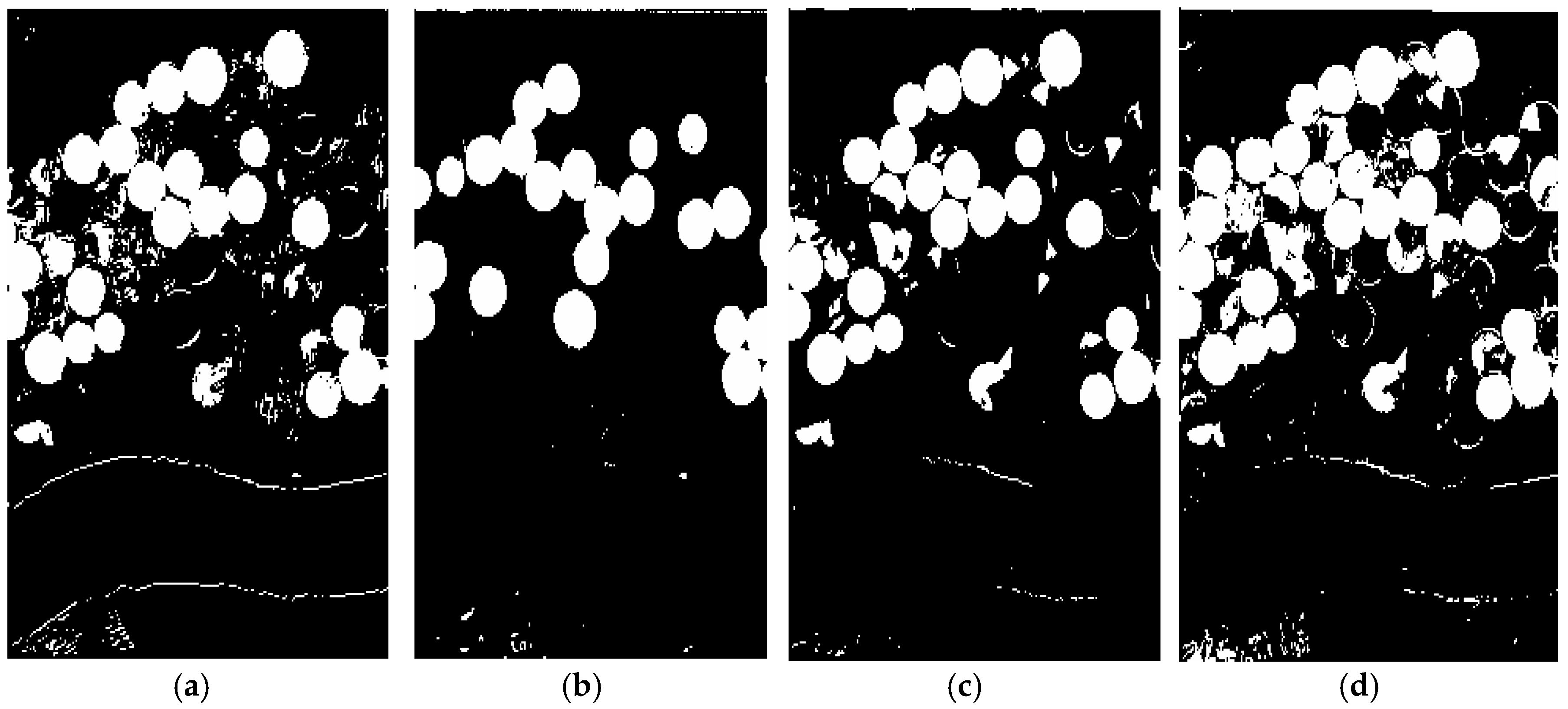
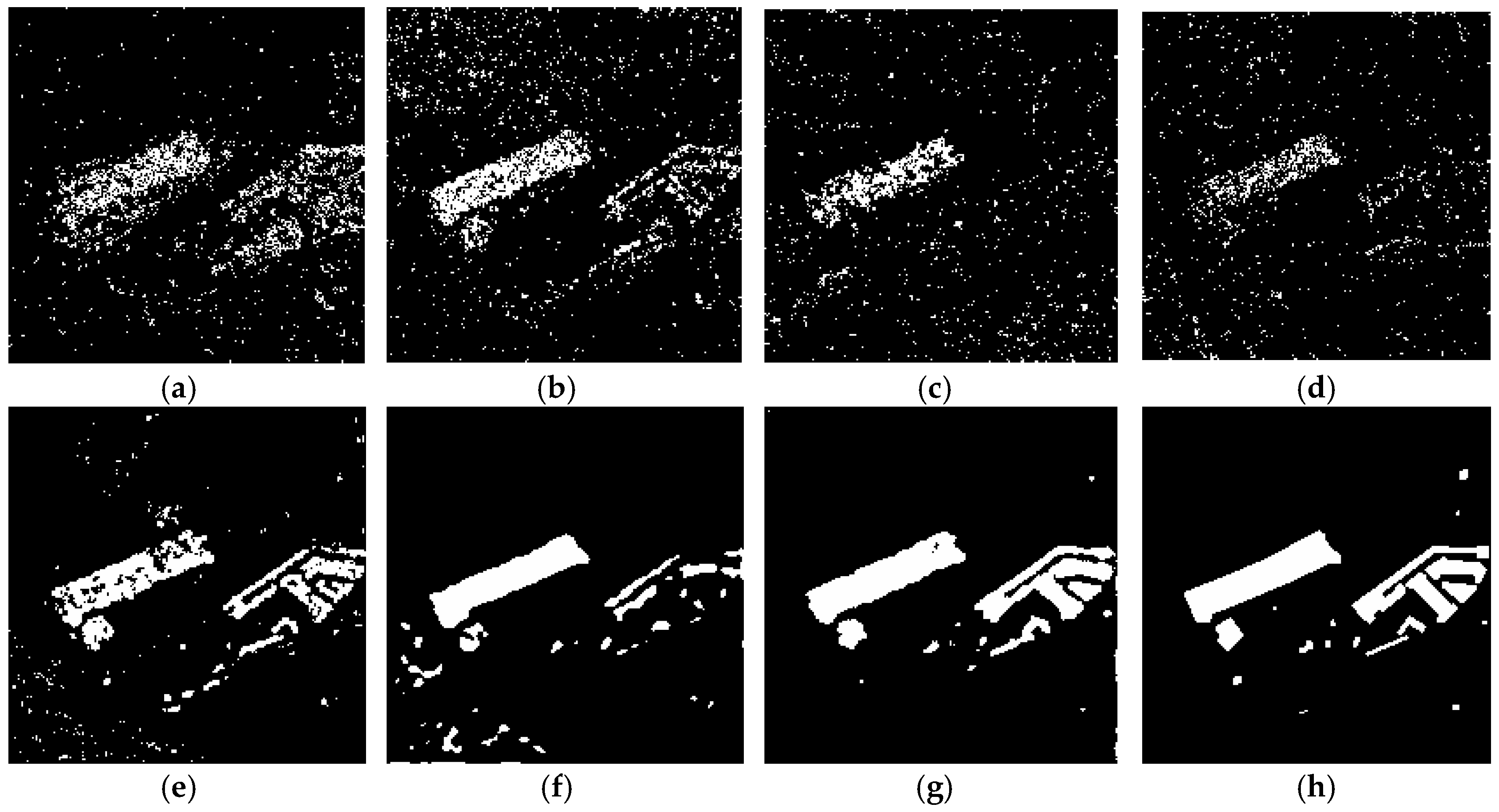
Figure 18.
The change detection maps of different methods for the Hyperspectral-Farmland dataset. (a) CVA-SVM, (b) MAD-SVM, (c) PCA-SVM, (d) IR-MAD -SVM, (e) SFA-SVM, (f) 3D-CNN, (g) Proposed Method, and (h) Ground Truth. White and black colors indicate the change and no-change areas, respectively.
Figure 18.
The change detection maps of different methods for the Hyperspectral-Farmland dataset. (a) CVA-SVM, (b) MAD-SVM, (c) PCA-SVM, (d) IR-MAD -SVM, (e) SFA-SVM, (f) 3D-CNN, (g) Proposed Method, and (h) Ground Truth. White and black colors indicate the change and no-change areas, respectively.
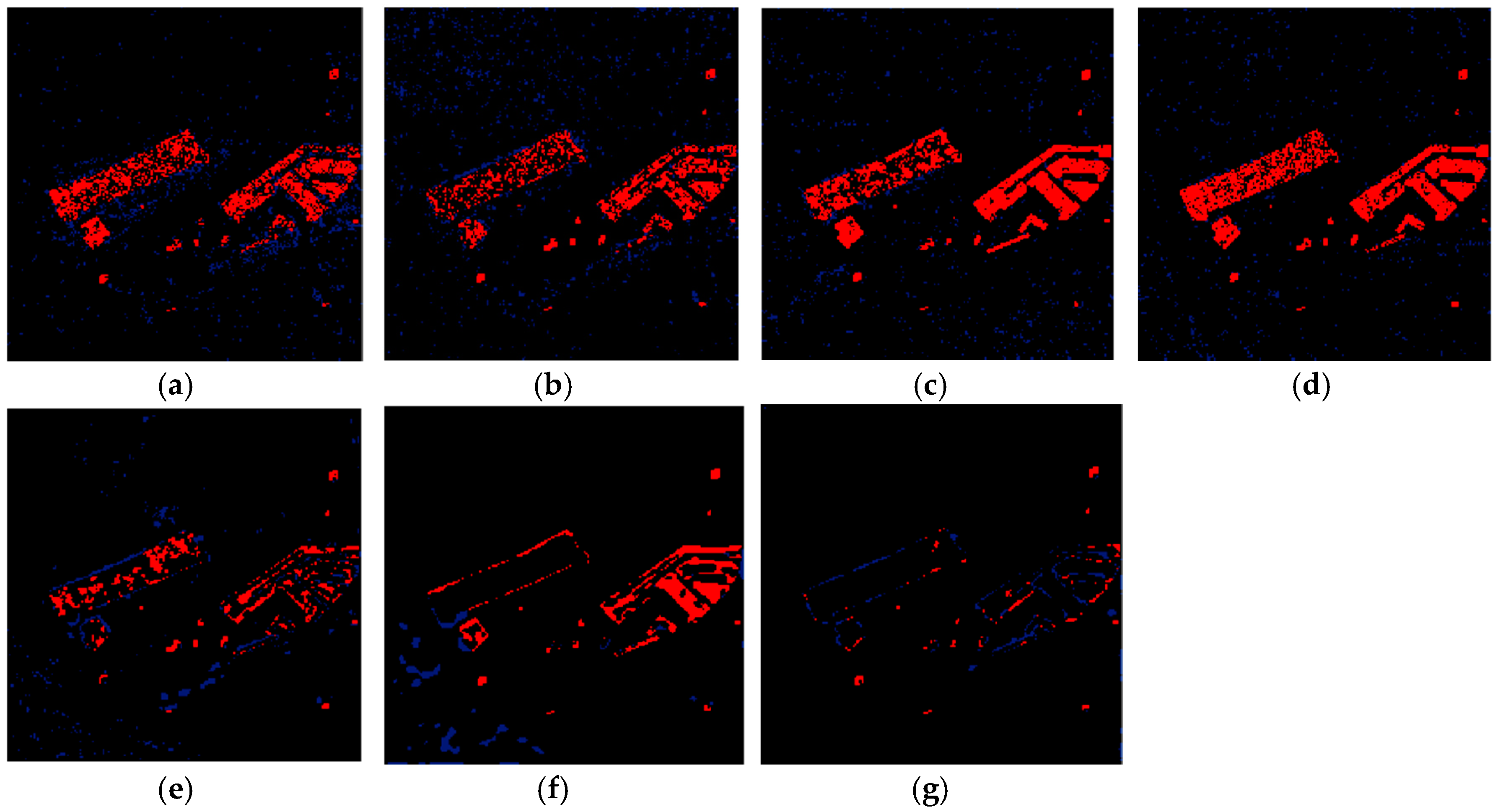
Figure 19.
The error in change detection maps obtained by different methods for the Hyperspectral-Farmland dataset. (a) CVA-SVM, (b) MAD-SVM, (c) PCA-SVM, (d) IR-MAD -SVM, (e) SFA-SVM, (f) 3D-CNN, and (g) Proposed Method. Black, red, and blue colors indicate TP and TN, FN, and FP pixels, respectively.
Figure 20.
The confusion matrices of different CD methods for the Hyperspectral-Farmland dataset. (a) CVA-SVM, (b) MAD-SVM, (c) PCA-SVM, (d) IR-MAD -SVM, (e) SFA-SVM, (f) 3D-CNN, and (g) Proposed Method.
Figure 20.
The confusion matrices of different CD methods for the Hyperspectral-Farmland dataset. (a) CVA-SVM, (b) MAD-SVM, (c) PCA-SVM, (d) IR-MAD -SVM, (e) SFA-SVM, (f) 3D-CNN, and (g) Proposed Method.
Figure 21.
The change detection maps of different methods for the PolSAR-San Francisco1 dataset. (a) CVA-SVM, (b) MAD-SVM, (c) PCA-SVM, (d) IR-MAD -SVM, (e) SFA-SVM, (f) 3D-CNN, (g) Proposed Method, and (h) Ground Truth. White and black colors indicate the change and no-change areas, respectively.
Figure 21.
The change detection maps of different methods for the PolSAR-San Francisco1 dataset. (a) CVA-SVM, (b) MAD-SVM, (c) PCA-SVM, (d) IR-MAD -SVM, (e) SFA-SVM, (f) 3D-CNN, (g) Proposed Method, and (h) Ground Truth. White and black colors indicate the change and no-change areas, respectively.
Figure 22.
The errors in change detection of different methods for the PolSAR-San Francisco1 dataset. (a) CVA-SVM, (b) MAD-SVM, (c) PCA-SVM, (d) IR-MAD -SVM, (e) SFA-SVM, (f) 3D-CNN, and (g) Proposed Method. Black, red, and blue colors indicate TN and TP, FN, and FP pixels, respectively.
Figure 22.
The errors in change detection of different methods for the PolSAR-San Francisco1 dataset. (a) CVA-SVM, (b) MAD-SVM, (c) PCA-SVM, (d) IR-MAD -SVM, (e) SFA-SVM, (f) 3D-CNN, and (g) Proposed Method. Black, red, and blue colors indicate TN and TP, FN, and FP pixels, respectively.
Figure 23.
The confusion matrices of different CD methods for the PolSAR-San Francisco1 dataset. (a) CVA-SVM, (b) MAD-SVM, (c) PCA-SVM, (d) IR-MAD -SVM, (e) SFA-SVM, (f) 3D-CNN, and (g) Proposed Method.
Figure 23.
The confusion matrices of different CD methods for the PolSAR-San Francisco1 dataset. (a) CVA-SVM, (b) MAD-SVM, (c) PCA-SVM, (d) IR-MAD -SVM, (e) SFA-SVM, (f) 3D-CNN, and (g) Proposed Method.
Figure 24.
The change detection maps of different methods for the PolSAR-San Francisco2 dataset. (a) CVA-SVM, (b) MAD-SVM, (c) PCA-SVM, (d) IR-MAD -SVM, (e) SFA-SVM, (f) 3D-CNN, (g) Proposed Method, and (h) Ground Truth. White and black colors indicate the change and no-change areas, respectively.
Figure 24.
The change detection maps of different methods for the PolSAR-San Francisco2 dataset. (a) CVA-SVM, (b) MAD-SVM, (c) PCA-SVM, (d) IR-MAD -SVM, (e) SFA-SVM, (f) 3D-CNN, (g) Proposed Method, and (h) Ground Truth. White and black colors indicate the change and no-change areas, respectively.
Figure 25.
The errors in change detection using different methods for the PolSAR- Francisco2 dataset. (a) CVA-SVM, (b) MAD-SVM, (c) PCA-SVM, (d) IR-MAD -SVM, (e) SFA-SVM, (f) 3D-CNN, and (g) Proposed Method. Black, red, and blue colors indicate TP and TN, FN, and FP pixels, respectively.
Figure 25.
The errors in change detection using different methods for the PolSAR- Francisco2 dataset. (a) CVA-SVM, (b) MAD-SVM, (c) PCA-SVM, (d) IR-MAD -SVM, (e) SFA-SVM, (f) 3D-CNN, and (g) Proposed Method. Black, red, and blue colors indicate TP and TN, FN, and FP pixels, respectively.
Figure 26.
The confusion matrices of different CD methods for the PolSAR-San Francisco2 dataset. (a) CVA-SVM, (b) MAD-SVM, (c) PCA-SVM, (d) IR-MAD -SVM, (e) SFA-SVM, (f) 3D-CNN, and (g) Proposed Method.
Figure 26.
The confusion matrices of different CD methods for the PolSAR-San Francisco2 dataset. (a) CVA-SVM, (b) MAD-SVM, (c) PCA-SVM, (d) IR-MAD -SVM, (e) SFA-SVM, (f) 3D-CNN, and (g) Proposed Method.
Table 1.
Description of multispectral datasets (italic characters are the name of datasets).
Table 1.
Description of multispectral datasets (italic characters are the name of datasets).
| Data | Resolution (m) | #Bands | Size (pixel) | Wavelength (nm) |
|---|
| Multispectral-Abudhabi | 10 | 13 | 401 × 401 | 356–1058 |
| Multispectral-Saclay | 10 | 13 | 260 × 270 | 356–1058 |
Table 2.
Description of hyperspectral datasets (italic characters are the name of datasets).
Table 2.
Description of hyperspectral datasets (italic characters are the name of datasets).
| Data | Resolution (m) | #Bands | Size (pixel) | Wavelength (nm) |
|---|
| Hyperspectral-River | 30 | 154 | 436 × 241 | 356–1058 |
| Hyperspectral-Farmland | 30 | 154 | 306 × 241 | 356–1058 |
Table 3.
The description of the Polarimetric Synthetic Aperture RADAR (PolSAR) datasets (italic characters are the name of datasets).
Table 3.
The description of the Polarimetric Synthetic Aperture RADAR (PolSAR) datasets (italic characters are the name of datasets).
| Dataset | Range Resolution (m) | Azimuth Resolution (m) | Incidence Angles (°) | Size (pixel) | Wavelength (cm) |
|---|
| PolSAR-San Francisco1 | 1.66 | 1.00 | [25,26,27,28,29,30,31,32,33,34,35,36,37,38,39,40,41,42,43,44,45,46,47,48,49,50,51,52,53,54,55,56,57,58,59,60,61,62,63,64,65] | 200 × 200 | 23.84 |
| PolSAR-San Francisco2 | 1.66 | 1.00 | [25,26,27,28,29,30,31,32,33,34,35,36,37,38,39,40,41,42,43,44,45,46,47,48,49,50,51,52,53,54,55,56,57,58,59,60,61,62,63,64,65] | 100 × 100 | 23.84 |
Table 4.
Confusion matrix (TP: True Positive, TN: True Negative, FP: False Positive, and FN: False Negative).
Table 4.
Confusion matrix (TP: True Positive, TN: True Negative, FP: False Positive, and FN: False Negative).
| Confusion Matrix | Predicted |
|---|
| Change | No-Change |
|---|
| Actual | Change | TP | FN |
| No-Change | FP | TN |
Table 5.
Different types of indices that were used for accuracy assessment of the change map produced using the proposed method by components TP, TN, FP, and FN (TP: True Positive, TN: True Negative, FP: False Positive, and FN: False Negative).
Table 5.
Different types of indices that were used for accuracy assessment of the change map produced using the proposed method by components TP, TN, FP, and FN (TP: True Positive, TN: True Negative, FP: False Positive, and FN: False Negative).
| Accuracy Index | Formula |
|---|
| OA | |
| Precision | |
| Sensitivity | |
| Specificity | |
| BA | |
| F1-Score | |
| MD | |
| FA | |
| KC | |
Table 6.
Numbers of samples for change detection in the six datasets used in this study.
Table 6.
Numbers of samples for change detection in the six datasets used in this study.
| Dataset | Class | Total Number of Pixels | Number of Samples | Percentage
(%) | Training | Validation | Testing |
|---|
| Multispectral-Abudhabi | Change | 11,519 | 2700 | 23.43 | 1755 | 405 | 540 |
| No-Change | 148,481 | 7500 | 5.05 | 4875 | 1125 | 1500 |
| Multispectral-Saclay | Change | 1610 | 500 | 31.06 | 325 | 75 | 100 |
| No-Change | 68,590 | 4900 | 7.14 | 3185 | 735 | 980 |
| Hyperspectral-River | Change | 9698 | 2200 | 22.68 | 1430 | 330 | 440 |
| No-Change | 101,885 | 5000 | 5.21 | 3250 | 750 | 1000 |
| Hyperspectral-Farmland | Change | 14,288 | 2000 | 14.00 | 1300 | 300 | 400 |
| No-Change | 59,458 | 2500 | 5.04 | 1625 | 375 | 500 |
| PolSAR-San Francisco1 | Change | 3434 | 810 | 23.58 | 527 | 121 | 162 |
| No-Change | 36,566 | 2400 | 6.56 | 1560 | 360 | 480 |
| PolSAR-San Francisco2 | Change | 1259 | 400 | 31.77 | 260 | 60 | 80 |
| No-Change | 8741 | 700 | 8.00 | 455 | 105 | 140 |
Table 7.
The optimum values for the training parameters of the proposed CNN network.
Table 7.
The optimum values for the training parameters of the proposed CNN network.
| Parameter | Bounding | Selected Value |
|---|
| Initial learning | {10−3, 10−4} | 10−4 |
| Epsilon value | {10−5, 10−9} | 10−9 |
| Number of epochs | {550,750,950} | 750 |
| Mini-batch size | {100,150} | 100 |
| Dropout rate | {0.1,0.2} | 0.1 |
| Patch size | {11,13} | 11 |
| Weight initializer | {Random, Glorot} | Glorot |
| Number of neurons at first full connected layer | {150,250} | 150 |
| Number of neurons at second full connected layer | {15,25} | 15 |
Table 8.
The accuracy of different change detection methods for the Multispectral-Abudhabi dataset (the best performance for each method appears in bold).
Table 8.
The accuracy of different change detection methods for the Multispectral-Abudhabi dataset (the best performance for each method appears in bold).
| Method | CVA | MAD | PCA | IR-MAD | SFA | 3D-CNN | Proposed Method |
|---|
| OA (%) | 80.54 | 91.80 | 88.08 | 91.79 | 92.54 | 91.73 | 98.89 |
| Sensitivity (%) | 61.94 | 9.10 | 45.85 | 10.30 | 16.82 | 0.59 | 96.65 |
| MD (%) | 38.06 | 90.90 | 54.15 | 89.70 | 83.18 | 99.41 | 3.35 |
| FA (%) | 18.01 | 1.78 | 8.64 | 1.88 | 1.59 | 1.20 | 0.93 |
| F1-Score (%) | 31.43 | 13.78 | 35.65 | 15.31 | 24.51 | 1.02 | 92.63 |
| BA (%) | 71.96 | 53.66 | 68.61 | 54.21 | 57.62 | 49.70 | 97.86 |
| Precision (%) | 21.06 | 28.39 | 29.17 | 29.81 | 45.14 | 3.68 | 88.93 |
| Specificity (%) | 81.99 | 98.22 | 91.36 | 98.12 | 98.41 | 98.80 | 99.07 |
| KC | 0.231 | 0.106 | 0.294 | 0.120 | 0.214 | 0.00 | 0.920 |
Table 9.
The accuracy of different change detection methods for the Multispectral-Saclay dataset (the best performance for each method appears in bold).
Table 9.
The accuracy of different change detection methods for the Multispectral-Saclay dataset (the best performance for each method appears in bold).
| Method | CVA | MAD | PCA | IR-MAD | SFA | 3D-CNN | Proposed Method |
|---|
| OA (%) | 94.09 | 91.05 | 92.55 | 91.1 | 92.48 | 98.15 | 99.18 |
| Sensitivity (%) | 19.50 | 42.48 | 19.25 | 40.56 | 31.06 | 29.19 | 75.40 |
| MD (%) | 80.50 | 57.52 | 80.75 | 59.44 | 68.94 | 70.81 | 24.60 |
| FA (%) | 4.16 | 7.81 | 5.72 | 7.70 | 6.07 | 0.23 | 0.25 |
| F1-Score (%) | 13.15 | 17.88 | 10.61 | 17.31 | 15.94 | 42.02 | 80.99 |
| BA (%) | 57.67 | 67.34 | 56.77 | 66.43 | 62.49 | 64.48 | 87.58 |
| Precision (%) | 9.92 | 11.32 | 7.32 | 11.00 | 10.72 | 74.96 | 87.46 |
| Specificity (%) | 95.84 | 92.19 | 94.28 | 92.30 | 93.93 | 99.77 | 99.75 |
| KC | 0.104 | 0.148 | 0.075 | 0.142 | 0.128 | 0.413 | 0.805 |
Table 10.
The accuracy of different change detection methods for the Hyperspectral-River dataset (the best performance for each method appears in bold).
Table 10.
The accuracy of different change detection methods for the Hyperspectral-River dataset (the best performance for each method appears in bold).
| Method | CVA | MAD | PCA | IR-MAD | SFA | 3D-CNN | Proposed Method |
|---|
| OA (%) | 96.41 | 93.51 | 96.75 | 87.13 | 92.94 | 95.02 | 97.50 |
| Sensitivity (%) | 77.76 | 36.52 | 77.35 | 59.89 | 70.21 | 76.47 | 81.66 |
| MD (%) | 22.23 | 63.47 | 22.64 | 40.10 | 29.78 | 23.52 | 18.33 |
| FA (%) | 1.81 | 1.06 | 1.40 | 10.27 | 4.89 | 3.21 | 0.99 |
| F1-Score (%) | 79.04 | 49.46 | 80.56 | 44.73 | 63.36 | 72.76 | 85.06 |
| BA (%) | 87.98 | 67.73 | 87.97 | 74.81 | 82.65 | 86.63 | 90.34 |
| Precision (%) | 80.37 | 76.63 | 84.05 | 35.69 | 57.72 | 69.39 | 88.74 |
| Specificity (%) | 98.19 | 98.94 | 98.60 | 89.72 | 95.10 | 96.78 | 99.01 |
| KC | 0.771 | 0.464 | 0.788 | 0.379 | 0.595 | 0.700 | 0.837 |
Table 11.
The accuracy of the different change detection methods applied to the Hyperspectral-Farmland dataset (the best performance for each method appears in bold).
Table 11.
The accuracy of the different change detection methods applied to the Hyperspectral-Farmland dataset (the best performance for each method appears in bold).
| Method | CVA | MAD | PCA | IR-MAD | SFA | 3D-CNN | Proposed Method |
|---|
| OA (%) | 95.93 | 85.81 | 96.06 | 91.23 | 94.87 | 94.91 | 97.15 |
| Sensitivity (%) | 85.55 | 47.47 | 82.13 | 86.91 | 76.82 | 82.84 | 90.78 |
| MD (%) | 14.44 | 52.52 | 17.86 | 13.08 | 23.17 | 17.15 | 9.21 |
| FA (%) | 1.59 | 5.04 | 0.619 | 7.73 | 0.824 | 2.21 | 1.329 |
| F1-Score (%) | 89.01 | 56.31 | 88.92 | 79.25 | 85.22 | 86.23 | 92.46 |
| BA (%) | 91.97 | 71.21 | 90.75 | 89.58 | 87.99 | 90.31 | 94.72 |
| Precision (%) | 92.76 | 69.22 | 96.94 | 72.83 | 95.69 | 89.91 | 94.21 |
| Specificity (%) | 98.40 | 94.96 | 99.38 | 92.26 | 99.17 | 97.78 | 98.67 |
| KC | 0.865 | 0.482 | 0.865 | 0.738 | 0.821 | 0.831 | 0.907 |
Table 12.
The accuracy of different change detection methods for the PolSAR-San Francisco1 dataset (the best performance for each method appears in bold).
Table 12.
The accuracy of different change detection methods for the PolSAR-San Francisco1 dataset (the best performance for each method appears in bold).
| Method | CVA | MAD | PCA | IR-MAD | SFA | 3D-CNN | Proposed Method |
|---|
| OA (%) | 91.74 | 92.17 | 91.36 | 91.37 | 95.64 | 95.62 | 98.31 |
| Sensitivity (%) | 44.11 | 52.62 | 27.57 | 22.56 | 71.75 | 64.00 | 93.06 |
| MD (%) | 55.88 | 47.37 | 72.42 | 77.43 | 28.24 | 35.99 | 6.93 |
| FA (%) | 3.78 | 4.11 | 2.64 | 2.16 | 2.11 | 1.41 | 1.19 |
| F1-Score (%) | 47.85 | 53.58 | 35.41 | 30.98 | 73.88 | 71.49 | 90.43 |
| BA (%) | 70.16 | 74.25 | 62.46 | 60.19 | 84.82 | 81.29 | 95.93 |
| Precision (%) | 52.27 | 54.57 | 49.47 | 49.42 | 76.14 | 80.95 | 87.94 |
| Specificity (%) | 96.21 | 95.88 | 97.35 | 97.83 | 97.88 | 98.58 | 98.80 |
| KC | 0.434 | 0.493 | 0.311 | 0.271 | 0.715 | 0.691 | 0.895 |
Table 13.
The accuracy of different change detection methods for the PolSAR-San Francisco2 dataset (the best performance for each method appears in bold).
Table 13.
The accuracy of different change detection methods for the PolSAR-San Francisco2 dataset (the best performance for each method appears in bold).
| Method | CVA | MAD | PCA | IR-MAD | SFA | 3D-CNN | Proposed Method |
|---|
| OA (%) | 88.28 | 89.68 | 89.76 | 89.23 | 91.73 | 93.87 | 95.89 |
| Sensitivity (%) | 9.85 | 22.16 | 26.93 | 17.95 | 40.98 | 57.27 | 79.03 |
| MD (%) | 90.15 | 77.84 | 73.07 | 82.05 | 59.02 | 42.73 | 20.97 |
| FA (%) | 0.42 | 0.59 | 1.19 | 0.50 | 0.96 | 0.86 | 1.68 |
| F1-Score (%) | 17.46 | 35.09 | 39.84 | 29.56 | 55.51 | 70.17 | 82.88 |
| BA (%) | 54.71 | 60.78 | 62.87 | 58.72 | 70.01 | 78.20 | 88.67 |
| Precision (%) | 77.02 | 84.29 | 76.52 | 83.70 | 86.00 | 90.58 | 87.13 |
| Specificity (%) | 99.57 | 99.40 | 98.81 | 99.50 | 99.04 | 99.14 | 98.32 |
| KC | 0.150 | 0.315 | 0.356 | 0.263 | 0.515 | 0.669 | 0.805 |
Table 14.
Comparison between the accuracies of the CD methods for CD in the Hyperspectral datasets (italic characters are the name of datasets).
Table 14.
Comparison between the accuracies of the CD methods for CD in the Hyperspectral datasets (italic characters are the name of datasets).
| Method | Hyperspectral-
River [29] | Hyperspectral-Farmland [3] | Proposed Method
Hyperspectral-River | Proposed Method
Hyperspectral-Farmland |
|---|
| OA (%) | 95.14 | 92.32 | 97.50 | 97.15 |
| KC | 0.754 | 0.818 | 0.837 | 0.907 |
Table 15.
Comparison between the accuracies of the CD methods for CD in the PolSAR datasets (italic characters are the name of datasets).
Table 15.
Comparison between the accuracies of the CD methods for CD in the PolSAR datasets (italic characters are the name of datasets).
| Method | PolSAR- Francisco1 [38] | PolSAR- Francisco2 [38] | PolSAR- Francisco1 [42] | Proposed Method
PolSAR- Francisco1 | Proposed Method
PolSAR- Francisco2 |
|---|
| OA (%) | 96.37 | 97.52 | 96.01 | 98.31 | 95.89 |
| KC | ---- | ---- | 0.762 | 0.895 | 0.805 |


