Review

Thermal Remote Sensing from UAVs: A Review on Methods in Coastal Cliffs Prone to Landslides

1
Department of Chemical and Geological Sciences, University of Cagliari, Cittadella Universitaria S.S. 554 bivio per Sestu I, 09042 Monserrato, CA, Italy
2
Department of Architecture, Built environment and Construction engineering, Politecnico di Milano, via Ponzio 31, 20133 Milano, Italy
3
Institute of Hydrogeology, Engineering Geology and Applied Geophysics, Charles University, Albertov 6, 128 43 Prague 2, Czech Republic
*
Author to whom correspondence should be addressed.
Remote Sens. 2020, 12(12), 1971; https://doi.org/10.3390/rs12121971
Submission received: 11 May 2020 / Revised: 14 June 2020 / Accepted: 17 June 2020 / Published: 19 June 2020
(This article belongs to the Collection Feature Papers for Section Environmental Remote Sensing)

Abstract

:
Coastal retreat is a non-recoverable phenomenon that—together with a relevant proneness to landslides—has economic, social and environmental impacts. Quantitative data on geological and geomorphologic features of such areas can help to predict and quantify the phenomena and to propose mitigation measures to reduce their impact. Coastal areas are often inaccessible for sampling and in situ surveys, in particular where steeply sloping cliffs are present. Uses and capability of infrared thermography (IRT) were reviewed, highlighting its suitability in geological and landslides hazard applications. Thanks to the high resolution of the cameras on the market, unmanned aerial vehicle-based IRT allows to acquire large amounts of data from inaccessible steep cliffs. Coupled structure-from-motion photogrammetry and coregistration of data can improve accuracy of IRT data. According to the strengths recognized in the reviewed literature, a three-step methodological approach to produce IRTs was proposed.

Graphical Abstract

1. Introduction

Landslides are ubiquitous, yet complex phenomena. As agents of localized erosion, they play an important role in landform evolution [1], counterbalancing relief-building processes and shaping drainage networks and coastlines [2]. They also are a remarkable source of risk for human life and economic assets—a risk that is projected to rise as world population increases, economy expands, and changes in global climate become more striking [3,4].
Landslides are a prime process driving the erosion and retreat of coastal cliffs [5,6,7]. They commonly occur as rock-and-soil falls, slides, avalanches or, less frequently, as topples or flows. Falling rocks from eroding cliffs can be especially dangerous to anyone occupying areas at their base or in nearby beaches [8]. The lithology and geological structure of the cliff exert the strongest control on landslide occurrence under continued weathering [6].
Regardless of the material involved—whether it be rock, debris or soil—gravity is the primary driver of landslide movement. On the other hand, the interplay of predisposing and causative factors that defines the mechanisms of initiation—and to some extent, also the fate of the moving mass—is not easily discernible [9,10]. Consequently, predicting the occurrence and dynamics of a landslide aiming at risk reduction is a highly complex task [11,12]. Landslide susceptibility is often assessed qualitatively, in a way entirely based upon the judgement of the person carrying out the analysis [13]. Recently, many efforts have been made to ensure a reduced level of subjectivity through novel rule-based systems [14].
Part of the complexity inherent to the initiation mechanism of a landslide and its forecasting can be resolved if appropriate information on the geological, geometric, hydraulic, mechanical, thermal, chemical and biologic characteristics (often intrinsically coupled), of the potentially unstable mass can be acquired and tracked through time [15,16]. Landslide monitoring through remote sensing is a vast subject that has been widely discussed from multiple viewpoints, sometimes focusing on specific applications such as mapping/inventorying, tracing multi-hazard chains and early warning [17,18,19,20,21]. Remote sensing methodologies are sometimes utilized in combination, so as to better exploit technique-specific strengths and reduce inherent shortcomings [22,23,24,25].
Landslides that initiate in inaccessible areas—such as coastal cliffs—can pose higher risks because their characterization and monitoring in the field is difficult or simply not feasible. In this context, remote sensing is an invaluable tool [26,27]. Structure-from-motion (SfM) photogrammetry from ground-based stations and unmanned aerial vehicles (UAVs) [28,29,30] allows the acquisition of large amounts of data from inaccessible areas, aiding in the identification of past, current and potential landslide structures and associated geometries, processes and affected lithologies. UAV-based SfM photogrammetry is particularly useful in steep cliffs, for which data acquisition from the ground is unfeasible, and sometimes the different points of view, gathered by these acquisitions, are not sufficient. Indeed, despite the high precision achievable, the main limitation of Terrestrial Laser Scanning (TLS) [31] for rock face monitoring are occlusions and shadowed areas that affect acquisition from faces with complex morphology. However, when applicable, TLS remains a solid technology that, coupled to methods for point-cloud-based deformation analysis [32], can produce very accurate results (see, e.g., [33]).
In the last two decades, the growing interest in the use of UAVs for geohazard monitoring has led to new methods with high spatial resolution and temporal accuracy [34,35,36,37]. Data interpretation may be performed, for instance with deep learning convolutional neural networks (CNNs) which overcome uncertainties related to the subjectivity of expert knowledge detection [38]. UAVs can rapidly provide information to evaluate structural damage and perform preliminary impact assessments during post-disaster emergency responses [39,40], but they remain precious tools in all phases of disaster management—from prevention to recovery [41,42,43,44]. In fact, UAVs are well suited for updating or producing ex novo high-resolution maps of areas where other aerial or spaceborne techniques cannot be implemented because of adverse weather conditions, lack of timeliness or excessive cost [45,46]. Although weather conditions may also affect the UAVs acquisitions, the flight can be rescheduled quickly, assuring in most cases a successful mission for data collection. UAVs have several desirable characteristics as they can reach remote locations and perform monitoring operations at various spatial scales with high temporal frequency. Moreover, they are able to acquire images at low altitude (<150 m above ground) with multiple views angles—thus enabling three-dimensional reconstructions—and they can be equipped with multiple sensors operating in different spectral ranges [22,47]. The availability of detailed spectral data promoted new approaches to characterize various geomaterials from their spectral signatures [48], providing both two-dimensional (2D) surface mapping and three-dimensional (3D) body information (e.g., lithological units and landslides masses) [49,50,51,52].
The ongoing downsizing of thermal infrared (TIR) sensor apparatuses has allowed a relevant improvement of UAVs capability in acquiring data for evaluating the stability of coastal cliffs and their short-term evolution. Thus, TIR applications have gained increasing interest and attention in the hazards research literature in the last years. The bibliometric analysis has highlighted the geographical and temporal distribution of published works on this topic. Three main databases, Scopus (www.scopus.com), Web of Science—WoS (webofknowledge.com) and Google Scholar (scholar.google.com/) were interrogated using a string of three combined keywords: “infrared thermography AND landslide OR rockfall”. These databases contain bibliographical information on books, articles and reviews, among others. Scopus and WoS feature only papers published in journals or conference proceedings of certified editors, whereas Google Scholar lists a variety of documents, including non-peer-reviewed technical reports. Hence, it can be used to understand the general trend of interest in a topic, more than the related scientific production.
A growing interest around TIR applications has been recognized, even though the dedicated scientific production is still in its infancy. The searches in Scopus, WoS and Google Scholar, in fact, returned 18, 20 and >500 results, respectively (Figure 1). The Scopus and WoS queries returned results from 2012–2020, whereas the ones from Google Scholar date back to 1973. However, only some documents found in Google Scholar appeared to fit well in the topic, such as “infrared thermography in landslides context”, while others only matched the combination of words. Nonetheless, the analysis shows a positive trend in the three databases, with an increasing number of documents published in the last years. Moreover, the geographical distribution of the results from WoS showed that most of the papers were published by teams of researchers entirely based in Italy, while only a few resulted from collaborations of Italy based researchers with colleagues in other countries. Keywords co-occurrence analysis [53] showed that infrared thermography is strictly linked to landslide and hazard, highlighting a scientific interest on this matter.
This review focuses, in particular, on algorithms and methods for the acquisition of geomechanical information from landslide-prone coastal cliffs in soil and rock using UAV-borne thermal infrared (TIR) sensors. By analyzing the recent literature, this study discusses the main issues related to the understanding of the thermal behavior of landslide-prone coastal cliffs—as it can be extracted from thermal data—and its correlation with geological features. Four main topics, that were identified as relevant for coastal cliff landslide investigations, will be examined: the type of geological and geomorphologic characteristics that can be inferred, the requirements in terms of thermal data acquisition by UAVs, the possible auxiliary data and co-registration, the processing effort and the expected accuracy. This study was proposed in the framework of the Project MAREGOT (MAnagement des Risques de l’Erosion cotière et actions de GOuvernance Transfrontalière—“Managing the Risks of Coastal Erosion and Cross-border Governance Actions) funded under the Maritime Programme: 2014–2020 INTERREG V-A Italy–France (http://interreg-maritime.eu/fr/web/maregot/projet). MAREGOT focuses on the joint prevention and management of the risks arising from coastal erosion in the Mediterranean area. A specific task, coordinated by the University of Cagliari (Italy), is dedicated to the assessment of cliff instability to understand the dynamics of erosive phenomena and coastlines, in relation to the geomorphologic and hydro-dynamic characteristics of the coasts. 3D point clouds using digital photogrammetry, terrestrial laser scanner and a thermal camera on board of a UAV were created. This activity, aiming at studying the instability of coastal cliffs, enhanced the requirement of a shared and complete methodology for the acquisition and interpretation of thermal data collected by UAVs in coastal environmental conditions [54].
The review is structured into the following sections: Thermal remote sensing techniques (Section 2), TIR data acquisition by UAVs (Section 3), IRT capabilities in landslide hazards (Section 4), IRT approaches in coastal rocky cliffs hazards (Section 5) and methodological synthesis on the basis of the present knowledge (Section 6).

2. Thermal Remote Sensing Techniques

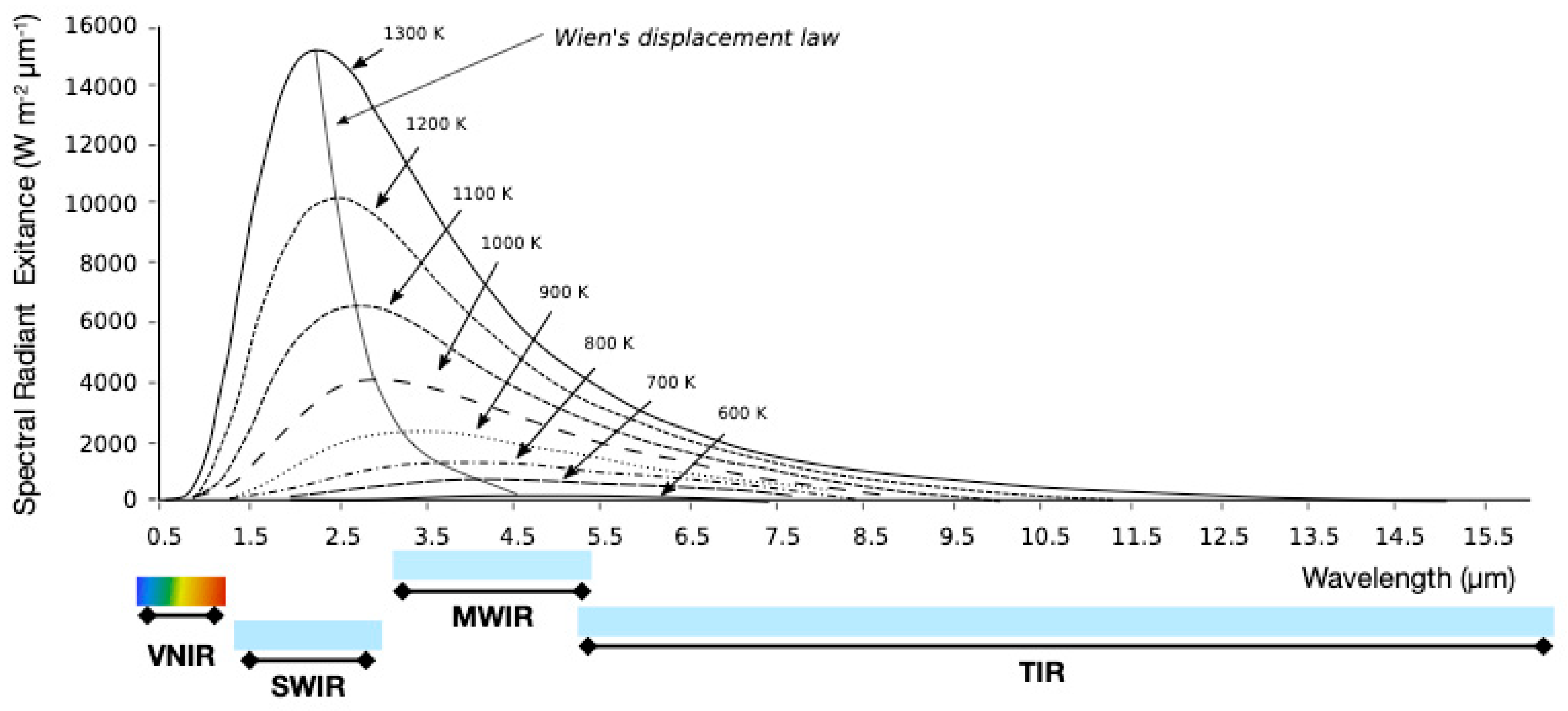
2.1. Thermal Infrared Domain

Thermal infrared imagery is commonly used to characterize land surface temperature (LST) and sea surface temperature (SST). In Figure 2, an example of thermal nighttime image highlighting the thermal behavior of different land covers is shown. The main aim of the study in the figure was to propose the monitoring of dust storms using the highest possible number of moderate resolution imaging spectroradiometer (MODIS) acquisitions (day and night) to forecast the potential affected urban areas [55,56].
With the increasing spatial and spectral resolution of thermal sensors, a large number of applications have been developed, thereby demonstrating the potential of utilizing thermal imaging data in natural and anthropic environments. These applications span from the identification of thermal anomalies linked to forest fires or coal fires to the quantification of water pollution or moisture contents, but also to machinery performance or heat dispersion from buildings in urban and industrial contexts [57].
Table 1 compares the TIR domain with other major spectral regions exploited for Earth Observation. The TIR wavelength domain, considering the entire spectral emission and capability to detect this radiation, has been classified into different ranges [57,58]. According to [59], it extends from about 3 to 14 μm, a range which refers in particular to that of the emitted energy detectable by sensors in the remote-sensing domain. In this range, all wavelengths are not completely transmitted through the atmosphere because of the presence of carbon dioxide, ozone and water vapor that absorb energy at certain wavelengths. Water vapor and carbon dioxide absorb radiation at 2.5–3 μm and 5–8 μm [60]. Consequently, two main TIR ranges are used, i.e., the 3–5 μm and 8–14 μm ranges, which are referred to as the “atmospheric windows”.

2.2. Interpreting Thermal Infrared Signals

The interpretation of thermal data are based on the understanding of the physical processes enabling the energy transfer, such as radiation [59]. All objects at a temperature above absolute zero (0 K, −273.15 °C) continuously emit electromagnetic radiation. The Earth surface, with an ambient temperature of ~300 K, has a peak energy emission in the TIR region at ~9.7 µm [59]. Sensors responsive in the thermal wavelengths have the capacity to record the TIR radiation emitted by surfaces that absorb a large part of the incoming solar radiation [57]. This radiant energy results from the conversion of the internal kinetic energy at molecular level. The electromagnetic energy radiated from a source is termed radiant flux and is measured in watts [W]. The kinetic temperature of an object can be measured with a thermometer placed in direct contact with it, whereas the radiant temperature, i.e., the density of the radiant flux, can be remotely measured by devices that detect the electromagnetic radiation in the TIR wavelength region [59]. The latter is quantified in terms of radiance per unit of wavelength and is referred to as spectral radiance [61].
The radiant flux is regulated by the Stefan–Boltzmann law, which states that the radiant flux density emitted by an object is proportional to the fourth power of the object’s surface temperature, implying that a hotter object will radiate much more energy than a cooler one. This law is applicable to all wavelengths of emission.
According to Wien’s displacement law, spectral radiant emissions show their peak wavelength at a shorter value with the temperature increasing:
λ m = A T
where λ m is the wavelength of maximum spectral exitance, A is Wien’s constant (i.e., 2897.8 μm K) and T is the absolute kinetic temperature (K).
Wien’s displacement law states that colder targets emit only a small amount of radiation compared to the hotter ones. This implies that thermal remote sensing at ambient temperature has to rely on small amounts of low-energy photons, which may be difficult to detect. Consequently, the spatial and spectral resolutions may have to be reduced when acquiring thermal data to ensure a reasonable signal-to-noise ratio.
The spectral radiance can be calculated according to Planck’s function (Equation (2)), which states that the spectral radiance emitted by a blackbody at a temperature T and wavelength λ can be calculated as:
L λ ( T ) = C 1 λ 5 ( e x p ( C 2 λ T ) 1 )
where C1 and C2 are constants, equal to 3.7413· 108 W m−2 μm4 and 1.4388·104 μm K, respectively [61].
The radiant emissions, according to Equation (1), can be detected by VNIR, SWIR, MIR and TIR sensors (Figure 3).
The application of Planck’s function relies on the assumption that a hypothetical body (termed blackbody) adsorbs and re-emits all energy incident upon it. The electromagnetic radiation emitted by a blackbody at a given wavelength is therefore only a function of the blackbody’s absolute temperature, following Kirchhoff’s law. However, real objects are not perfect emitters or absorbers, thus Planck’s function is modified by an emission-efficiency factor, termed emissivity ( ε ). This is a function of the wavelength [60] and can be defined as:
ε = F r F b
where Fr and Fb are the radiant fluxes from a real material and from a blackbody, respectively. As a consequence, a blackbody will have ε = 1, while all real materials ε < 1 (generally between 0.7–0.95). In real materials, a high value of ε signifies that a large proportion of incident energy is absorbed and radiated back, while the opposite holds true for materials with low ε [59].
The interaction between the incident radiant flux (irradiance) and an object results in three coefficients, measured by the ratio of reflected, absorbed and transmitted radiant fluxes and the irradiance, respectively: reflectance (ρ), absorbance (α) and transmittance (τ).
Considering the principle of energy conservation, if for a blackbody, at a given wavelength, the emittance is equal to the absorbance, i.e.:
ε ( λ ) = α ( λ )
so that the sum of α, ρ and τ equals 1 (as most objects are opaque and do not transmit), the following equation can be formulated:
ε ( λ ) + ρ ( λ ) = 1
Using Equation (5), the spectral emittance can be calculated from the reflectance, and vice versa.
The relationship between the spectral radiant emission and temperature of the emitting surfaces is of particular interest, for instance, in volcanology, as the temperature of volcanic features varies in a wide range [62,63]. Through thermal remote sensing, volcanic activity and eruptions can be monitored and hazard assessments can be performed accordingly [64,65,66].
Using the emissivity, the Stefan–Boltzmann law can be rewritten as:
T ( r a d ) = ε ( 1 / 4 ) T ( k i n ) ε ( λ ) + ρ ( λ )
so that the radiant temperature (T(rad)) can be converted into kinetic temperature (T(kin)).
Because ε < 1 in real materials, from Equation (6) it results that the remotely sensed T(rad) is always lower than the locally measurable T(kin) on the material’s surface. However, if the material’s ε is known, the real T(kin) can be calculated. For a first-order analysis, tabular data of emissivity for various materials, such as metals, nonmetals, common construction materials, minerals and rocks, water and vegetation can be used. However, the emissivity of a material is a function of temperature and surface geometry (also intended as surface finish, roughness), thus tabular data should only be used as a guide or for indicative comparative measures. The emissivity of the specific material under investigation should always be experimentally determined when absolute and detailed measurements are required [60,61].
Moreover, because the spectral emissivity changes according to the wavelength and angle of incidence [67], the emissivity spectra should be collected using multispectral and hyperspectral spectrometers either remotely and in a controlled environment.

2.3. Remotely Sensed TIR Application in Geological Domains

Recently, the expression “thermal infrared imagery” has been replaced with “infrared thermography” (IRT) [59]. A thermography is a map of surface temperature and is derived from TIR images. Thermal sensors detect the radiant energy emitted by the land surface. This energy is transmitted (not absorbed) through the atmosphere, but also emitted by the atmosphere itself. The remote-sensing interpretation of the land–atmosphere signal is complicated by this coupling, yet a thermography still allows the estimation of several environmental variables useful in Earth System Science modeling [68]. The emissivity is informative of the composition of the radiant surface, and is a fundamental parameter in atmospheric and energy-balance models, as it must be known alongside with the radiant temperature to establish the heat measure of the surface [69]. Starting from the TIR radiance recorded by the sensor, an apparent temperature or surface radiant temperature is assigned to each pixel. This process is based on the application of corrections for the effects of atmospheric radiance and TIR instrument sensor gains, offsets and sensitivities. As aforementioned, the surface radiant temperature is not only a function of the surface temperature, but also of the surface emissivity. Moreover, if the emissivity of the surface is known, the surface kinetic temperatures can be calculated using the relation among radiance, emissivity and temperature. The contribute of the emissivity are generally corrected by classifying the optical channels of an image into surface type classes and assigning an emissivity value to each class [57]. Some interesting results were obtained for urban areas by applying the Temperature and Emissivity Separation (TES) algorithm, originally developed for the advanced spaceborne thermal emission and reflection radiometer (ASTER) spaceborne sensor [70] and used to provide an accurate emissivity map using data provided by the airborne hyperspectral scanner (AHS) [71]. Detailed emissivity correction is recommended to retrieve accurate values of surface temperature [72,73,74,75]. In [75], the main multichannel and single-channel algorithms to extract the LST and land surface emissivity (LSE) are discussed in detail.
The mineral characterization from thermal spectra was first demonstrated in the 1960s in laboratory. The selective emission of thermal radiation from minerals, rocks and soils was exploited to identify mineral groups, such as silicates, carbonates, sulfates and phosphates [76]. The first multichannel thermal scanner for mapping geological units (the Dedalus 24-channel scanner) was developed in the late 1970s. Since the 1980s, TIR sensors have been utilized in different contexts, such as mining and tunneling, detection of hydrological features in karst watersheds, monitoring of geothermal activity, mapping of geomorphologic and sedimentary features of alluvial fans, agricultural soil analysis for moisture content and LST monitoring [77,78,79,80,81,82,83].
The first thermal sensor for remote-sensing acquisitions (the thermal infrared multispectral scanner, TIMS) was released in 1981 [84]. On the basis of the performance of these sensors, the possibility of developing a spaceborne sensor for multichannel thermal measurements within the Landsat program was considered [85]. The Jet Propulsion Laboratory (under a NASA contract), in collaboration with the Japanese Space Agency and the Ministry of Trade and Industry of Japan, developed and launched the advanced spaceborne thermal emission and reflection radiometer (ASTER) onboard of the Terra satellite in 1990 [86]. From this period on, the use of TIR remotely sensed data have found important applications in the geological domain for the recognition of minerals, especially in mining surveys [49,87,88]. ASTER can acquire 5 bands in the TIR domain (see Table 2), permitting to enhance the spectral components of minerals and apply complex algorithms for the processing of geological models. The ground sample distance (GSD) of these bands is 90 m (https://asterweb.jpl.nasa.gov/characteristics.asp). Several band ratios have been proposed to map mineral indices using ASTER bands. The ASTER team, for instance, proposed an empirical silica index using ASTER TIR bands [86].
As all materials radiate energy at various TIR wavelengths, the temperature of an object can be measured both during daytime hours and during the night. This capability relates to the thermal inertia, a measure of the thermal response of a material to variations of its temperature. The thermal inertia depends on the thermal conductivity and specific heat capacity, and is proportional to the material density [59,73]. Soils and rocks with higher thermal inertia, such as sandstone and quartzite, tend to show smaller variations of surface temperature during a circadian solar heating cycle compared to materials with lower thermal inertia such as shale, gravel and pyroclastic covers. The thermal inertia cannot be measured by remote sensing directly, whereas it can be measured through field or laboratory tests. However, proxies such as the day–night difference of temperature (DT) and the Apparent Thermal Inertia (related to the albedo in the visible band), which are retrievable through remote sensing, have been successfully utilized for soil moisture monitoring [74].

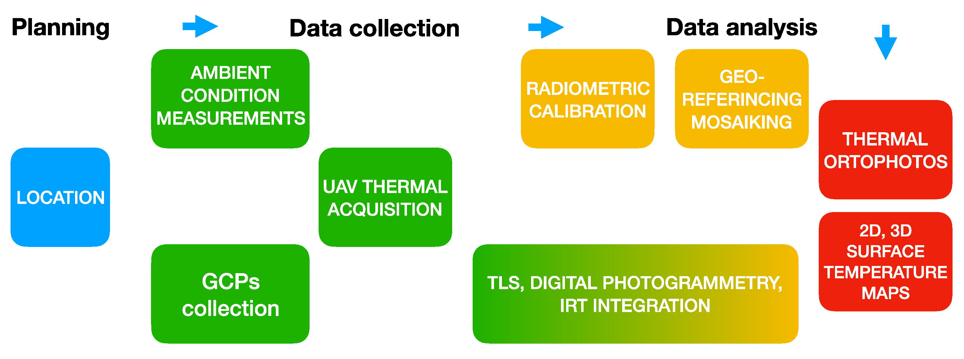
3. Thermal Data Acquisition by UAVs

Remote-sensing sensors can be differentiated in terms of their spatial resolution, which constrains the field and scale of their application. Spaceborne remotely sensed imagery has an immense potential as an enabling tool for the generation of spatial maps. Spaceborne instruments provide an advantage for collecting data continuously and, in general, at regional scale, yet they still cannot match the spatial detail or temporal resolution achievable using airborne sensors. Aircrafts with adequate fight duration can map large areas even in a single flight mission. Interesting studies on the application of airborne TIR in urban areas to classify vegetation and soil moisture have been reported [89].
The flexibility of the surveying and the ability to reach inaccessible and hazardous areas such as active volcanoes has promoted the use of UAVs in the last years [90,91]. They can nowadays carry sensors for detailed surveys throughout moderate-sized areas while remaining compact and low-cost compared with manned aircrafts. UAVs combine the characteristics of short (and flexible) revisit time and high spatial resolution, thus they are well suited for detailed multitemporal observations [92,93]. Most of the advances in geomatics have indeed been achieved when relatively large areas could be mapped in the visible and NIR bands using compact cameras [94,95,96]. In a recent research, the combined use of IRT and UAVs [97] has made it possible to investigate frequent instability phenomena connected with weathering in steep tuff slopes.
In proximal sensing, i.e., when UAV-mounted or ground-based cameras are employed, the GSD is a fundamental parameter for appropriate surveying, as the sensor-object distance controls the achievable resolution [98]. In fact, the thermal sensor registers an at-sensor radiance ( L a t s e n s o r [W m−2]) per each pixel, which is a function of the surface radiance ( L s u r f ) and the attenuation by the atmosphere ( L a t m ) [99,100]:
L a t s e n s o r = t · L s u r f + L a t m
where t is the atmospheric transmittance (dimensionless; 0 < t < 1).
Both t and L a t m mainly depend on the atmospheric water content and the sensor-object distance [100]. It has been suggested that during the overfly of the airborne vehicle (as for spaceborne acquisitions), ground truth calibration may be appropriate to evaluate the sensor accuracy [57,101].
In Table 3, the technical specifications of the thermal imaging cameras utilized in landslide studies discussed in this study are shown. These thermal cameras are equipped with detectors sensitive to IR radiation at 7–14 µm wavelength. The incoming radiation heats the detector and changes its electrical resistance, which is measured and converted into temperature values. Different thermal cameras have different pixel pitch, sensor resolution and radiometric resolution.
The potential of UAV-based IRT mainly arises from the high resolution of the images, their low cost and portability [102]. The spatial image resolution is the highest at short distances. Common thermal imaging cameras have a geometric resolution (Instantaneous Field Of View-IFOV) ranging from 0.65 mrad to 2 mrad at 1 m distance, resulting in a ground resolution as high as 2 × 2 mm [103,104]. To analyze an entire slope, it is necessary to mount the thermal camera on a UAV in order to expand the FOV, and the resolution of the thermal imaging results in centimetric values [102].

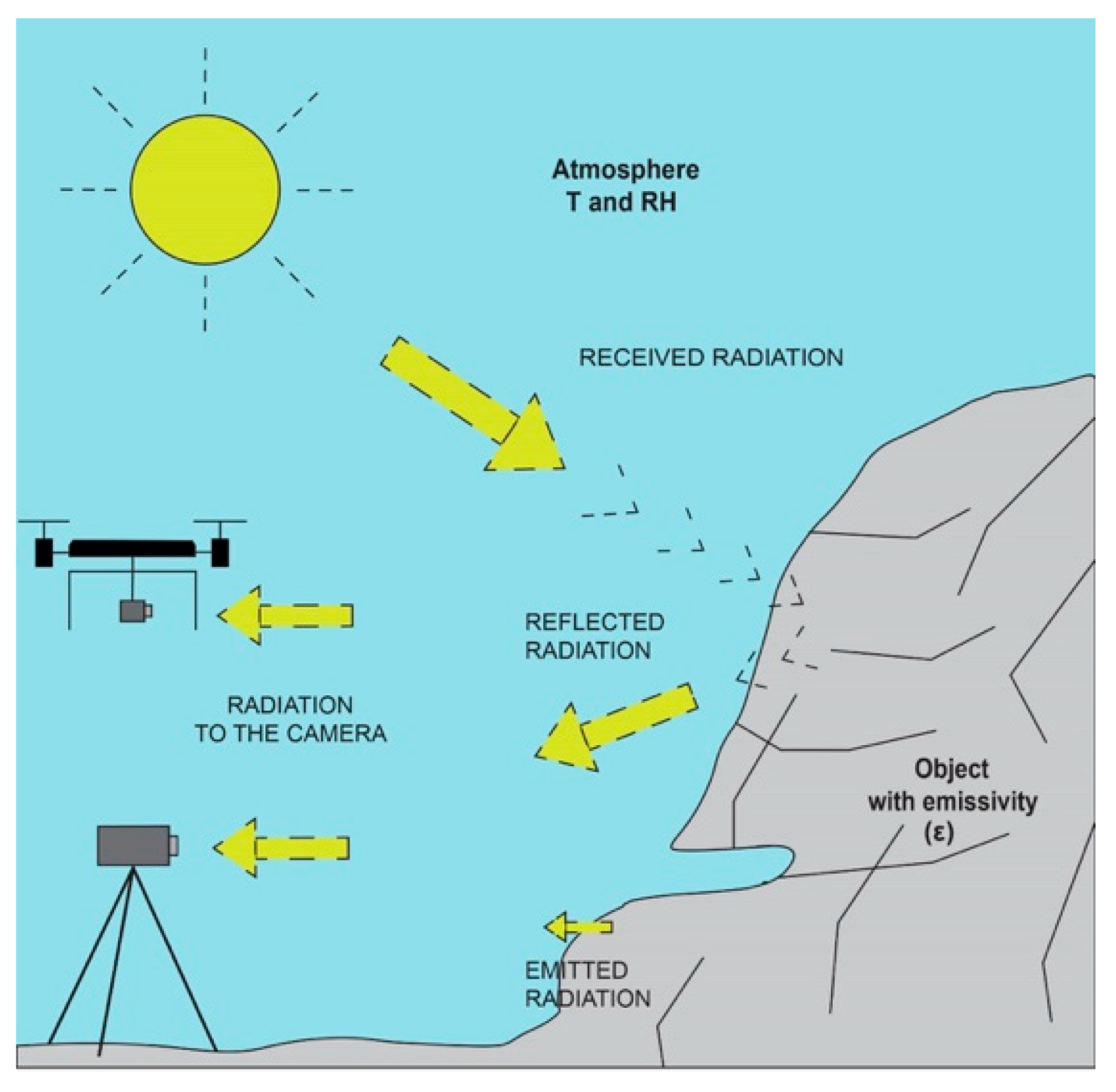
3.1. Data Processing: Atmospheric Correction

The kinetic temperature of an object, its emissivity and atmospheric effects control the intensity of the radiation detected by the thermal camera. Before the acquisition, specific camera settings are thus suggested to minimize measurement errors [112]. The recorded radiation is a function of the surface temperature of the object, but also depends on the radiation emitted by the atmosphere, which is higher when the air temperature is higher [113]. The camera automatically compensates multiples parameters, whereas some others need to be defined by the user in relation to the distance between the object and the sensor, namely: the reflected apparent temperature, the atmospheric transmission and the air temperature [67] (Figure 4).
The reflected apparent temperature refers to the thermal radiation that originates from another body but is reflected by the object and recorded by the camera. It is especially significant when the emissivity is low [57].
As for the atmospheric transmission, common methodologies to account for this phenomenon in both single- and multichannel acquisitions from large distances have been described in the literature [115]. On the other hand, specific studies tackling atmospheric effects at short distances, which are relevant for IRT acquisitions from UAVs, are still limited, possibly because other environmental conditions, such as wind speed and humidity, are given priority in research as they can have a stronger influence on the measure [112]. Nonetheless, simulations of thermography acquisition during flights at different altitudes actually demonstrated that a lack of atmospheric correction can lead to important errors, even for short object-sensor distances [116]. Errors larger than 4 K in conditions of high relative humidity and low air temperature were in fact evaluated at a distance of 150 m [116]. The application of the MODerate resolution atmospheric TRANsmission (MODTRAN) radiative model for the correction of atmospheric effects could reduce the Root Mean Square Error (RMSE) of the temperature evaluation to less than 1 K. In the model, the atmosphere could be treated as a single-layer medium with uniform conditions because the variability of atmospheric parameters could be neglected in the altitude range of the observations.
The air temperature also influences the propagation of radiation. However, if the object-sensor distance is small and the flight altitude is less than 30 m, the radiometric distortion caused by the atmosphere may be neglected [112]. In most studies entailing proximal sensing, the atmospheric effects were simply compensated by defining a single air temperature value in the camera settings [114].

3.2. Data Processing: Geometric Correction

Optical remotely sensed images are commonly processed to obtain digital elevation models and orthophotos with very high resolution using photogrammetric techniques. Photogrammetry refers to the methodology of extracting three dimensional data from photographs [117]. The reconstruction of the 3D geometry of a rock cliff requires the use of images at large photo-scale that need to be collected in its proximity and at various points of view. As already mentioned, UAVs give the opportunity to collect such images. The other fundamental advance is provided by the Structure-from-Motion (SfM) algorithms, that make the orientation and calibration of the camera fully automatic, without any a priori knowledge on the location of camera stations [30,118,119]. Thanks to the Multi-view Dense Matching, once the mutual position of the camera poses is reconstructed, a detailed point cloud describing the surface of the recorded object can be automatically obtained. The model is also directly textured with the radiometric content of the images, opening to the use of virtual/augmented reality techniques that allow to carry out some analyses by simulating on site conditions (see, e.g., [120]).
While the term SfM should refer to the image orientation phase only, it is now commonly used to address the whole photogrammetric process, especially in geosciences [121]. The 3D-point clouds generated in this process can be referred to a coordinate-system model using few ground control points (GCPs), which need to be laid out in the field and georeferenced using geodetic techniques (global navigation satellite system (GNSS) and total stations) before the UAV acquisition. It is essential that the GCPs are clearly recognizable in the overlapping images– an operation that is based on manual measurements unless coded targets of suitable size are used [122]. An alternative solution to the use of GCPs consists in the direct georeferencing of the adopted drone, that should be equipped with GNSS-RTK (real-time kinematic) sensors [123] or other types of precise positioning systems [124].
The SfM technique was used extensively to process optical (RGB) imagery, yet its applicability is not limited to it. Most software packages also allow for the processing of multi- and hyperspectral imagery, including thermal imagery [100,125,126,127,128,129]. Specifically, most acquisitions from commercial thermal cameras can be processed by using the same camera model as for optical images [94,117].
Thermal data are sometimes processed through SfM to generate orthophotos [100,130,131]. However, the limited pixel contrast in thermal images compared to RGB images often hinders the SfM processing [132,133,134]. In such cases, thermal maps can still be generated manually, by mosaicking the separate images individually georeferenced using GCPs. The number and distribution of GCPs have a direct influence on the resulting accuracy, being necessary at least three GCP per image, but preferably a higher number (e.g., at least six per image). Nonetheless, in various environments, the limited visibility of GCPs and the complexity of their measurement may pose major problems. For this reason, some authors proposed the concurrent acquisition of optical and thermal images. Optical data are used to reconstruct the surface geometry, but also to allow the extraction of those GCPs necessary for the orientation of each thermal image by using an integrated bundle adjustment [135]. Solutions for the integrated automatic processing of interspectral images has also been proposed [136] in order to obtain aligned outputs from optical and thermal data.
The use of artificial GCPs can be necessary in thermal images as it is sometimes difficult to identify well-defined natural points. Aluminum sheets, which do not need power supply, are often utilized because of their sharp boundary in thermal images [137,138]. They reflect almost 90% of the thermal radiation in the atmosphere [139] and exhibit a low absorbed intensity, appearing dark in thermal images [137,140]. This way, even though thermal images have high blur and low contrast, a spatial accuracy similar to that of optical images can still be achieved. Sometimes, targets with different composition and colors are also used [112], while reference targets with known temperature are employed for radiometric calibration [141].

3.3. Auxiliary Data and Coregistration Processing

In geological applications, thermal data can be used for the identification of landforms, lithologies and structural features. Optical and TLS sensors are widely used to map and monitor slope instabilities, and can be used in co-registration with data from other sensors, such as thermal sensors, to enhance the slope characterization [94,142,143,144]. Methodologies that incorporate object-based image analysis (OBIA) with two machine learning (ML) methods, namely the multilayer perceptron neural network (MLP-NN) and random forest (RF), have been developed for landslide detection [145]. Data on distances, volumes, horizontal and vertical coordinates of objects can be extracted [146]. Photogrammetry from UAVs has been applied successfully to characterize rockfall movements [147,148,149].
The alignment of point clouds obtained from TLS and thermal data can be obtained by using GCPs, with similar drawbacks as in the case of coregistration of optical and thermal images. The automatic fusion of thermal images and 3D models has been successfully exploited in the case of buildings, but its application to geological surfaces may be difficult because of their higher irregularity [124,150,151].
Other solutions have been based on the development of integrated sensors, which in general show low flexibility due to different acquisition geometry [152].

4. IRT Capabilities in Landslide Hazards

IRT-based studies for landslide assessment began in the early 2000s, when high-resolution thermal cameras became available. In this context, IRTs were first performed from ground-based platforms in combination with TLS, geophysical investigations and traditional field surveys. TIR images overlapped to 3D models, generated from TLS surveys, are used for faster data interpretation and analysis [33]. The ability to record small variations in IR radiation has the advantage of extending the observation capability to a variety of processes which are sensitive to minor temperature variations. Therefore, in recent years, IRT has proven to be a strong tool for modeling the geological behavior of unstable rock masses [102,106,107,153,154,155,156,157,158,159,160].
With reference to thermal remote sensing in geological studies, as already discussed, one of the most interesting applications entails the use of multispectral TIR emissions to extract spectral properties of rocks from their emissivity spectra. Unfortunately, common thermal sensors mounted on UAVs only function in one or two thermal bands, limiting the ability to identify minerals and physical characteristics of the surfaces. Therefore, most of the applications of TIR data in geological hazard studies have focused on the mapping and monitoring of floods, landslides and coastal inundation hazards [161]. For landslide detection, high-resolution thermal cameras can provide high-definition thermograms, supporting the identification of fractures, water and weathered areas [162] (Figure 5).
More recently, sensors with even higher resolution have improved the estimation of geomechanical characteristics of rock slopes, supporting field surveying and laboratory testing [102,162]. It has been shown [67] that IRT can provide objective and quantitative information on anomalies and thermal variations in relation to differences of moisture in rock outcrops, which may lead to detachments. Water infiltration in rock masses, discontinuity networks, and debris covers may be identified by interpreting thermal anomalies [102]. Furthermore, multitemporal thermographic measurements, by operating in different lighting conditions, may achieve evaluations on the thermal efficiency of the rocks [106,158].
The analysis of rock mass features is an essential step to understand rockfall and toppling phenomena. Field methods to detect rock mass discontinuities follow the approaches described in [163,164]. The scanline method [164] is one of the field strategy to measure and describe rock mass features. Many studies have explored the relationship between mechanical properties and thermal behavior. For instance, it has been shown through laboratory analysis [109] that differences in porosity of intact volcanic rocks may control their cooling behavior. Recent research efforts are thus focusing on the thermal behavior of fractured rock masses and on the capacity of IRT to predict some geo-mechanical features on the basis of thermal anomalies of the discontinuities.
As discussed in [67,107,165], thermal imaging systems can be useful in preliminary evaluations of discontinuity systems. It has been demonstrated that the presence of voids in the rock, due to its porosity or to rock failures, may be correlated to different values of emitted temperature. The temperature values during the heating and cooling phases have been used to correlate the trend of each specimen with the corresponding porosity value. One of the first studies exploiting thermal data for rock-mass description was carried out by Wu [106], who demonstrated the capacity of the different parts of a rock mass, with dissimilar structural and morphologic characteristics, to warm up and release heat in different ways. In the context of rockfalls, this technique was applied to a limestone underground mine in northern Spain to quantify the risk of rockfalls during mine exploitation [67].
A method based on the analysis of a series of thermal images (thermograms or thermographic images) acquired during rock-cliff cooling at night–time has been proposed by Zaragoza et al. [156] and implemented in MATLAB- MathWorks Inc. environment [166]. The authors motivated the data acquisition during rock cooling as direct sun heating would have induced high disturbance, with significant noises due to the relative position between the source and the facets of the surface. Even more, Guerin et al. [167] demonstrated that by repeating IRT surveys during cooling and heating phases, the thermal anomalies can be highlighted because they are strongly controlled by the degree of fracturing and weathering of the rock. Indeed, in coastal environment weathering for sea spray plays a more relevant role in downgrading mechanical quality of the rock mass than in inland environments.
A 3D visualization is often beneficial for the accurate identification of structural characteristics. Ultimately, the reconstruction of the discontinuity networks allows to constrain the geological volumes of potentially unstable rock wedges, which is a necessary step for planning landslide risk reduction and monitoring measures [102]. This reconstruction is not always possible, as some characteristics of the rock mass are difficult to detect, yet IRT can be of great aid, as the high thermal contrast between the environment and the fractures can be exploited for their detection [159,167]. In fact, the air or water circulation in the open fractures allows to detect their temperature. With dry conditions, the temperature of the air in the fractures can be significantly higher than the surface air temperature, resulting in a significant heat flux anomaly from the rock [108]. The heating of a fracture is a function of its opening. In fact, very open fractures allow the passage of hot air flows, while tight or filled discontinuities exhibit much lower thermal intensity. Groundwater flow usually cools down fractured zone, particularly in the summertime. Both dry and wet condition produce thermal anomalies within the rock mass providing information on the degree of interconnection of the fractures and their persistence, which is often difficult to determine with direct field surveys [114]. In coastal environment this difference is enhanced by the higher thermal range. Moreover, a correlation between the fracturing degree of the rock mass and the cooling behavior has been detected. A cooling rate index (CRI) has been proposed to identify one area with respect to another for its cooling capacity during a specific time window. According to the evidence, the index could be used as a tool to remotely detect the rock quality, as a linear correlation between CRI and jointing. In this way, preliminary estimates of the slope conditions could be done [114].
Depending on the time of the day in which the measurement is performed, the fracturing system emits higher or lower radiation than the intact rock. As the cooling of the rock mass depends by the temperature difference with the external environment, nocturnal analyses during the cooling phase have been considered to offer the best conditions for obtaining well-defined thermograms [57,114]. In fact, after the sunset, parasite radiation is absent and the temperature difference between the objects and air is the highest. Moreover, on daytime thermographic acquisitions, external radiation emitted by other bodies can cast shadows on the slope under investigation, producing a signal bias. Therefore, before an investigation, the rock mass exposure and the timing of the acquisition must be carefully evaluated [114]. In the analyzed literature, nighttime conditions proved to be the best for the definition of thermograms [107,114,160,168].
Soil slopes may also exhibit important temperature-dependent behaviors, not only in seasonally cold regions under freeze-thawing cycles, but also under thermal excursions typical of temperate areas or in response to extreme heating caused, for instance, by wildfires [169,170]. The amplitude of the thermal signal in the soil, driven by solar irradiance and surface air temperature oscillations, damps with depth considerably, so that circadian and seasonal oscillations typically penetrate only to depths of some decimeters or a few meters, respectively. However, specific conditions such as important sub vertical groundwater flows or the presence of open fractures may increase the penetration depth remarkably. Moreover, longer-period climate trends, such as the natural centennial variability and the anthropogenic climate change, may locally induce significant variations of temperature at larger depths in human time scales [171]. In landslide assessment, however, changes of temperature are generally only accounted for indirectly and changes in patterns and frequency of landslides in response to climate change are mostly attributed to variations in precipitation patterns [1,4], whereas field and experimental evidence of landslides directly activated by changes in soil temperature have indeed been reported [172,173].
The systematic overlooking of thermally induced processes relevant to soil slope stability originates from the fact that the mechanisms by which temperature affects the mechanical properties of soils are diverse and not completely understood. The behavior of soil slopes is controlled by the interplay of coupled hydro-mechanical processes, which are especially pronounced in clay-rich materials. Various studies have shown that variations of temperature may affect both the hydraulic and mechanical aspects of clay behavior [174]. The properties of water—flowing in the pores and adsorbed on the particle surface—are temperature-dependent, thereby affecting the way the soil responds to external loads. As water, air and soil particles have different thermal properties, changes of temperature can also alter pressures and stresses within the soil [175]. Loss of apparent cohesion can occur in unsaturated soils as temperature increases—driven by a loss of water retention capacity—and structural collapse has also been reported [176,177]. Various frameworks have been proposed to describe the thermo-hydro-mechanical behavior of soils. However, their application to land surface processes is still in its infancy, as tools for upscaling the constitutive relations to the slope and regional scales are being developed [178]. In this context, the availability of remotely sensed thermal data from IRT, coupled with soil-moisture information, vegetation coverage, land surface geometry and precipitation patterns, can be a precious tool for model development and validation, as well as an essential input in absence of densely distributed ground-based and borehole monitoring.

5. IRT Approaches in Coastal Rocky Cliffs Hazards

Coastal instability is generally related to the interaction of marine and gravitational processes as well as the accelerated weathering effects due to sea spray. For this reason, coastal cliffs can be considered vulnerable, given the connection with more parameters compared with inland landslides [54,179,180,181,182,183]. Rockfalls occur commonly in high coasts, and they are among the faster landslide movements. These movements suffer from two principal factors: gravity and discontinuities distribution [184]. Additional movements along the coastal slopes can be recognized in the form of translational and rotational landslides in soil and debris. Due to their nature, damages in surrounding areas are highly possible. At the same time, rapid flows have the same potential as fast movements. Hard-rock coastal cliffs, e.g., granite, are often affected by weathering phenomena that lead to the formation of debris deposits in some portions of the slope, which could be mobilized as debris slides and flows. The evaluation of the magnitude of these landslide phenomena becomes fundamental in environmental management and hazard monitoring [5,6,185]. Collecting data and implement monitoring systems in coastal environments is a challenge, mainly where high cliffs with a steep cliff gradient are present.
In recent years, investigation techniques on coastal landslides have been developed with the contribution of new remote sensing tools [179,182,186,187,188,189,190,191]. Currently, however, there are no well-defined investigation protocols. Existing studies often do not follow uniform methodologies, mainly due to the lack of knowledge and complexity in collecting data on the processes that generate coastal erosion [181,185,192]. Principal applications of the IRT in coastal landslides hazard are aimed at detection of main discontinuities, main cavities, loosen/altered materials and identification of soil moisture and groundwater flows [162,168].
Even from large distances, it is possible to distinguish the volumes of landslide bodies thanks to thermal contrasts (Figure 5). Unstable areas can be recognized by processing thermal images taken at different irradiation moments during the day, thanks to the higher ability of the landslide body to transfer thermal energy compared to the surrounding rocks, due to the presence of an air circulation system inside the voids [102]. Through proximal sensing analysis, it has been demonstrated that it is possible to highlight the contrasts of thermal energy emitted between the fracturing system and the intact rock [158] and also to infer the main geotechnical parameters from cliff discontinuity set information according to the response in terms of surface thermal radiation.
Thermal cameras coupled with UAVs can be advantageous in studying the stability of vertical cliffs, as they allow to keep multi-view acquisitions with respect to the object-sensor, with a consequently higher value of thermal radiation [102]. The reliability of IRT to the study of inaccessible areas as coastal cliffs is pointed out by Mineo [160].
An update of Pappalardo et al. [168] proved the possibility of determining source areas as rock wedges. The camera resolution is such that information on the fracturing system, due to the joints opening, can be provided at mm–cm scale. The contrasts between the discontinuity system and weak areas, probably underwent decompression phenomena after the initial wedge sliding can help to identify areas which would lead to retreat phenomenon of the slope. In their study, the results seem to be clearer in summer acquisitions [168].
The integration of thermography with ground-based interferometric synthetic aperture radar (GBinSAR) and TLS in coastal cliffs is discussed in [193], with reference to the stability analysis of a coastal cliff in southern Italy. In particular, IRT results show the detachments as areas with a concentration of thermal anomalies. These results suggest the need for an integrated approach of remote sensing techniques to propose the model of slope instability in complex areas like coastal cliffs, where the partial and side visibility may be considered the main issue.

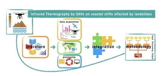
6. Methodological Synthesis and Conclusions

A comparison among the relevant methods to characterize coastal cliffs affected by landslides is provided in Table 4. The factors (constraints) influencing the phases of the planning, the data collection, the data analysis and the results have been evaluated for each technique: Traditional field survey, TLS, photogrammetry and IRT. An evaluation of strengths and weakness of each method has been provided.
Thermography with UAVs, integrated with TLS or photogrammetry data, compared to traditional field survey, proved to be a useful non-invasive technique in slope instability studies as evidenced in literature (see the Table 4). The potential of UAV thermography for coastal cliffs characterization can be recognized in the production of rock mass images of medium/high resolution, in the low-cost and easy portability [110]. All the proposed techniques were proved to be useful for the reconstruction of the fracture network. Indeed, the higher spatial resolution of the data collected by TLS and photogrammetric techniques can be integrated by the capacity to characterize the geotechnical behavior of the rock mass. Weather conditions may affect the UAV’s flight and the TLS acquisitions. Moreover, considering the visibility of the objects, IRT at the latitude of northern hemisphere, is more effective in summer season. Due to higher solar radiation, the heating phase is faster than in winter, during the night the cooling phase is slower, and thermal anomalies are higher [114]. Using these data, geomechanical features (i.e., fractures network, RQD) and physical properties of rock masses (i.e., porosity, bulk density) may be correlated to thermograms [109].
On the basis of the methods discussed in the analyzed literature, an approach to produce IRTs is hereby proposed (Figure 6). The methodology consists of three main steps: planning, data collection and data analysis.
The planning step comprises the analysis of the location, including the evaluation of accessibility issues. In this perspective, the orientation of the slope and UAV limitations (restricted airspace and logistic problems) have to be taken into account [165]. Moreover, nighttime acquisition should be considered, if achievable [107,109,154,168].
The data collection phase begins with the positioning of ground control points and the acquisition of their position [195]. At the same time, ambient-sensitive parameters such as object emissivity, path length, humidity and air temperature must be considered prior to the UAV flight [196]. If possible, auxiliary data as TLS and optical images should be acquired [193].
In the data analysis phase, thermal data are managed through software tools. For instance, the FLIR tool is a software package that allows to visualize, edit, and perform radiometric calibrations [112]. The SfM can also be applied [122,156,197]. Performing mosaicking and georeferencing is possible in a GIS environment, combining thermal snapshots with digital photogrammetric data (DEM). The coupling of IRT with TLS allows to obtain 3D models capable of showing various properties of the slope comprehensively, generating orthophotos at the same time [102,198].
This review highlights that the application of thermal remote sensing to coastal landslides is a new, but promising field of study. The publications cited throughout the study can be considered as a guide to apply a correct approach, adapting the environmental conditions to the specific coastal cliffs’ domain. As shown in Table 5, most of the published studies entailed the use of a thermal camera mounted on a tripod for terrestrial acquisition. The literature on UAV-mounted cameras is still scarce. The main geological and morphologic features highlighted in these studies concerned the identifications of weathered areas and fracture networks, cavities and pseudo-karst caverns, recently collapsed areas, landslide bodies, as well as the evaluation of shallow inhomogeneities and moisture content patterns. Resolution of cameras on the market provide UAV-based IRT a likelihood of getting an accurate measurement of fracture patterns, thus being a valuable support to the in situ surveys in coastal steep area, where collecting samples and performing direct measurements are often impossible. Accuracy of data can be improved coupling UAVs-based SfM photogrammetry and IRT methods and implementing a coregistration data system.

Author Contributions

For this research, the following represents author contributions to this manuscript. Conceptualization, M.T.M., S.D.P., A.F., M.S., and G.S.; Formal Analysis, M.T.M., S.D.P., M.S., and G.S.; Investigation, I.E., M.L., G.D., V.D., M.A.M., and F.D.; methodology, M.T.M., S.D.P., I.E., M.L., G.D., and M.A.M.; Writing—Original Draft Preparation, M.T.M., S.D.P., I.E., M.L., M.S., and G.S.; writing—review & Editing, M.T.M., S.D.P., and G.S.; supervision, M.T.M.; funding acquisition, M.T.M., S.D.P., A.F., and G.S.; project administration, A.F. and G.S. All authors have read and agreed to the published version of the manuscript.

Funding

This review was funded by Project MAREGOT (MAnagement des Risques de l’Erosion cotière et actions de GOuvernance Transfrontalière–Managing the Risks of Coastal Erosion and Cross-border Governance Actions) under the Program: 2014–2020 INTERREG V-A Italy - France (Maritime). G. Scaringi acknowledges financial support by the Czech Science Foundation (GAČR Junior Grant No. GJ20-28853Y).

Conflicts of Interest

The authors declare no conflicts of interest.

References

  1. Crozier, M. Landslide geomorphology: An argument for recognition, with examples from New Zealand. Geomorphology 2010, 120, 3–15. [Google Scholar] [CrossRef]
  2. Korup, O.; Densmore, A.L.; Schlunegger, F. The role of landslides in mountain range evolution. Geomorphology 2010, 120, 77–90. [Google Scholar] [CrossRef]
  3. Froude, M.J.; Petley, D.N. Global fatal landslide occurrence from 2004 to 2016. Nat. Hazards Earth Syst. Sci. 2018, 18, 2161–2181. [Google Scholar] [CrossRef] [Green Version]
  4. Gariano, S.L.; Guzzetti, F. Landslides in a changing climate. Earth Sci. Rev. 2016, 162, 227–252. [Google Scholar] [CrossRef] [Green Version]
  5. Dong, P.; Guzzetti, F. Frequency-Size Statistics of Coastal Soft-Cliff Erosion. J. Waterw. Port Coast. Ocean Eng. 2005, 131, 37–42. [Google Scholar] [CrossRef] [Green Version]
  6. Bromhead, E.; Ibsen, M.-L. Bedding-controlled coastal landslides in Southeast Britain between Axmouth and the Thames Estuary. Landslides 2004, 1, 131–141. [Google Scholar] [CrossRef]
  7. Hapke, C.J. Estimation of regional material yield from coastal landslides based on historical digital terrain modelling. Earth Surf. Process. Landf. 2005, 30, 679–697. [Google Scholar] [CrossRef]
  8. Haque, U.; Da Silva, P.F.; Devoli, G.; Pilz, J.; Zhao, B.; Khaloua, A.; Wilopo, W.; Andersen, P.; Lu, P.; Lee, J.; et al. The human cost of global warming: Deadly landslides and their triggers (1995–2014). Sci. Total Environ. 2019, 682, 673–684. [Google Scholar] [CrossRef]
  9. Tiranti, D.; Nicolò, G.; Gaeta, A.R. Shallow landslides predisposing and triggering factors in developing a regional early warning system. Landslides 2018, 16, 235–251. [Google Scholar] [CrossRef]
  10. Conforti, M.; Pascale, S.; Robustelli, G.; Sdao, F. Evaluation of prediction capability of the artificial neural networks for mapping landslide susceptibility in the Turbolo River catchment (northern Calabria, Italy). Catena 2014, 113, 236–250. [Google Scholar] [CrossRef]
  11. Soeters, R.; van Westen, C.J. Slope instability recognition, analysis, and zonation. In Landslides, Investigation and Mitigation Transportation Research Board, National Research Council, Special Report; Turner, A.K., Schuster, R.L., Eds.; National Academy Press: Washington, DC, USA, 1996; Volume 247, pp. 129–177. ISBN 0-309-06151-2. [Google Scholar]
  12. Manconi, A.; Giordan, D. Landslide failure forecast in near-real-time. Geomat. Nat. Hazards Risk 2014, 7, 1–10. [Google Scholar] [CrossRef] [Green Version]
  13. Fell, R.; Corominas, J.; Bonnard, C.; Cascini, L.; Leroi, E.; Savage, W.Z. Guidelines for landslide susceptibility, hazard and risk zoning for land use planning. Eng. Geol. 2008, 102, 85–98. [Google Scholar] [CrossRef] [Green Version]
  14. Roodposhti, M.S.; Aryal, J.; Pradhan, B. A Novel Rule-based Approach in Mapping Landslide Susceptibility. Sensors 2019, 19, 2274. [Google Scholar] [CrossRef] [Green Version]
  15. Angeli, M.-G.; Pasuto, A.; Silvano, S. A critical review of landslide monitoring experiences. Eng. Geol. 2000, 55, 133–147. [Google Scholar] [CrossRef]
  16. Tarchi, D.; Casagli, N.; Fanti, R.; Leva, D.D.; Luzi, G.; Pasuto, A.; Pieraccini, M.; Silvano, S. Landslide monitoring by using ground-based SAR interferometry: An example of application to the Tessina landslide in Italy. Eng. Geol. 2003, 68, 15–30. [Google Scholar] [CrossRef]
  17. Guzzetti, F.; Mondini, A.C.; Cardinali, M.; Fiorucci, F.; Santangelo, M.; Chang, K.-T. Landslide inventory maps: New tools for an old problem. Earth Sci. Rev. 2012, 112, 42–66. [Google Scholar] [CrossRef] [Green Version]
  18. Fiorucci, F.; Giordan, D.; Santangelo, M.; Dutto, F.; Rossi, M.; Guzzetti, F. Criteria for the optimal selection of remote sensing optical images to map event landslides. Nat. Hazards Earth Syst. Sci. 2018, 18, 405–417. [Google Scholar] [CrossRef] [Green Version]
  19. Joyce, K.; Belliss, S.; Samsonov, S.; McNeill, S.; Glassey, P. A review of the status of satellite remote sensing and image processing techniques for mapping natural hazards and disasters. Prog. Phys. Geogr. Earth Environ. 2009, 33, 183–207. [Google Scholar] [CrossRef] [Green Version]
  20. Pirasteh, S.; Li, J. Landslides investigations from geoinformatics perspective: Quality, challenges, and recommendations. Geomat. Nat. Hazards Risk 2016, 8, 448–465. [Google Scholar] [CrossRef] [Green Version]
  21. Fan, X.; Scaringi, G.; Korup, O.; West, A.J.; Van Westen, C.; Tanyas, H.; Hovius, N.; Ran, J.; Jibson, R.W.; Allstadt, K.E.; et al. Earthquake-Induced Chains of Geologic Hazards: Patterns, Mechanisms, and Impacts. Rev. Geophys. 2019, 57, 421–503. [Google Scholar] [CrossRef] [Green Version]
  22. Luo, Y.; Jiang, W.; Li, B.; Jiao, Q.; Li, Y.; Li, Q.; Zhang, J. Analyzing the formation mechanism of the Xuyong landslide, Sichuan province, China, and emergency monitoring based on multiple remote sensing platform techniques. Geomat. Nat. Hazards Risk 2020, 11, 654–677. [Google Scholar] [CrossRef] [Green Version]
  23. Kyriou, A.; Nikolakopoulos, K. Assessing the suitability of Sentinel-1 data for landslide mapping. Eur. J. Remote Sens. 2018, 51, 402–411. [Google Scholar] [CrossRef] [Green Version]
  24. Jiménez-Perálvarez, J.D.; El Hamdouni, R.; Palenzuela, J.A.; Irigaray, C.; Chacón, J. Landslide-hazard mapping through multi-technique activity assessment: An example from the Betic Cordillera (southern Spain). Landslides 2017, 14, 1975–1991. [Google Scholar] [CrossRef]
  25. Türk, T. Determination of mass movements in slow-motion landslides by the Cosi-Corr method. Geomat. Nat. Hazards Risk 2018, 9, 325–336. [Google Scholar] [CrossRef] [Green Version]
  26. Scaioni, M. Introduction. In Modern Technologies for Landslide Monitoring and Prediction; Scaioni, M., Ed.; Springer Natural Hazards; Springer: Berlin/Heidelberg, Germany, 2015; pp. 1–9. ISBN 978-3-662-45931-7. [Google Scholar]
  27. Fan, X.; Xu, Q.; Scaringi, G.; Li, S.; Peng, D. A chemo-mechanical insight into the failure mechanism of frequently occurred landslides in the Loess Plateau, Gansu Province, China. Eng. Geol. 2017, 228, 337–345. [Google Scholar] [CrossRef]
  28. Colomina, I.; Molina, P. Unmanned aerial systems for photogrammetry and remote sensing: A review. ISPRS J. Photogramm. Remote Sens. 2014, 92, 79–97. [Google Scholar] [CrossRef] [Green Version]
  29. Granshaw, S.I. RPV, UAV, UAS, RPAS … or just drone? Photogramm. Rec. 2018, 33, 160–170. [Google Scholar] [CrossRef]
  30. Westoby, M.; Brasington, J.; Glasser, N.F.; Hambrey, M.; Reynolds, J. ‘Structure-from-Motion’ photogrammetry: A low-cost, effective tool for geoscience applications. Geomorphology 2012, 179, 300–314. [Google Scholar] [CrossRef] [Green Version]
  31. Vosselman, G.; Maas, H.G. Airborne and Terrestrial Laser Scanning; CRC Press: Boca Raton, FL, USA, 2010; ISBN 978-1-904445-97-6. [Google Scholar]
  32. Lindenbergh, R.C.; Pietrzyk, P. Change detection and deformation analysis using static and mobile laser scanning. Appl. Geomat. 2015, 7, 65–74. [Google Scholar] [CrossRef]
  33. Scaioni, M.; Roncella, R.; Alba, M.I. Change Detection and Deformation Analysis in Point Clouds. Photogramm. Eng. Remote Sens. 2013, 79, 441–455. [Google Scholar] [CrossRef]
  34. Hamshaw, S.D.; Engel, T.; Rizzo, D.M.; O’Neil-Dunne, J.; Dewoolkar, M.M. Application of unmanned aircraft system (UAS) for monitoring bank erosion along river corridors. Geomat. Nat. Hazards Risk 2019, 10, 1285–1305. [Google Scholar] [CrossRef] [Green Version]
  35. Cao, C.; Liu, D.; Singh, R.P.; Zheng, S.; Tian, R.; Tian, H. Integrated detection and analysis of earthquake disaster information using airborne data. Geomat. Nat. Hazards Risk 2015, 7, 1–30. [Google Scholar] [CrossRef] [Green Version]
  36. Deffontaines, B.; Chang, K.-J.; Champenois, J.; Fruneau, B.; Pathier, E.; Hu, J.-C.; Lu, S.-T.; Liu, Y.-C. Active interseismic shallow deformation of the Pingting terraces (Longitudinal Valley–Eastern Taiwan) from UAV high-resolution topographic data combined with InSAR time series. Geomat. Nat. Hazards Risk 2016, 8, 120–136. [Google Scholar] [CrossRef] [Green Version]
  37. Turner, D.; Lucieer, A.; De Jong, S.M. Time Series Analysis of Landslide Dynamics Using an Unmanned Aerial Vehicle (UAV). Remote Sens. 2015, 7, 1736–1757. [Google Scholar] [CrossRef] [Green Version]
  38. Ghorbanzadeh, O.; Meena, S.R.; Blaschke, T.; Aryal, J. UAV-Based Slope Failure Detection Using Deep-Learning Convolutional Neural Networks. Remote Sens. 2019, 11, 2046. [Google Scholar] [CrossRef] [Green Version]
  39. Fan, X.; Xu, Q.; Scaringi, G.; Dai, L.; Li, W.; Dong, X.; Zhu, X.; Pei, X.; Dai, K.; Havenith, H.-B. Failure mechanism and kinematics of the deadly June 24th 2017 Xinmo landslide, Maoxian, Sichuan, China. Landslides 2017, 14, 2129–2146. [Google Scholar] [CrossRef]
  40. Fan, X.; Xu, Q.; Scaringi, G.; Zheng, G.; Huang, R.; Dai, L.; Ju, Y. The “long” runout rock avalanche in Pusa, China, on August 28, 2017: A preliminary report. Landslides 2018, 16, 139–154. [Google Scholar] [CrossRef]
  41. Murphy, R.R.; Steimle, E.; Griffin, C.; Cullins, C.; Hall, M.; Pratt, K. Cooperative use of unmanned sea surface and micro aerial vehicles at Hurricane Wilma. J. Field Robot. 2008, 25, 164–180. [Google Scholar] [CrossRef]
  42. Pratt, K.S.; Murphy, R.R.; Stover, S.; Griffin, C. CONOPS and autonomy recommendations for VTOL small unmanned aerial system based on Hurricane Katrina operations. J. Field Robot. 2009, 26, 636–650. [Google Scholar] [CrossRef]
  43. Molina, P.; Colomina, I.; Vitoria, T.; Silva, P.F.; Skaloud, J.; Kornus, W.; Prades, R.; Aguilera, C. Searching Lost People with UAVs: The System and Results of the CLOSE-SEARCH Project. ISPRS Int. Arch. Photogramm. Remote Sens. Spat. Inf. Sci. 2012, 441–446. [Google Scholar] [CrossRef] [Green Version]
  44. Griffin, G.F. The Use of Unmanned Aerial Vehicles for Disaster Management. Geomatica 2014, 68, 265–281. [Google Scholar] [CrossRef]
  45. Boccardo, P.; Chiabrando, F.; Dutto, F.; Tonolo, F.G.; Lingua, A. UAV Deployment Exercise for Mapping Purposes: Evaluation of Emergency Response Applications. Sensors 2015, 15, 15717–15737. [Google Scholar] [CrossRef] [PubMed] [Green Version]
  46. Fan, X.; Scaringi, G.; Xu, Q.; Zhan, W.; Dai, L.; Li, Y.; Pei, X.; Yang, Q.; Huang, R. Coseismic landslides triggered by the 8th August 2017 Ms 7.0 Jiuzhaigou earthquake (Sichuan, China): Factors controlling their spatial distribution and implications for the seismogenic blind fault identification. Landslides 2018, 15, 967–983. [Google Scholar] [CrossRef]
  47. Giordan, D.; Manconi, A.; Remondino, F.; Nex, F. Use of unmanned aerial vehicles in monitoring application and management of natural hazards. Geomat. Nat. Hazards Risk 2017, 8, 1–4. [Google Scholar] [CrossRef]
  48. De Souza, M.K.; Tognoli, F.M.W.; Veronez, M.R.; De Oliveira, L.P.L.; Gonzaga, L.; Cagliari, J.; Scaioni, M. High-resolution spectroscopy for detecting stratigraphic surfaces and stacking patterns in sedimentary basins. J. South Am. Earth Sci. 2018, 88, 287–293. [Google Scholar] [CrossRef]
  49. Gomez, C.; Delacourt, C.; Allemand, P.; Ledru, P.; Wackerle, R. Using ASTER remote sensing data set for geological mapping, in Namibia. Phys. Chem. Earth Parts A B C 2005, 30, 97–108. [Google Scholar] [CrossRef]
  50. Yu, L.; Porwal, A.; Holden, E.-J.; Dentith, M.C. Towards automatic lithological classification from remote sensing data using support vector machines. Comput. Geosci. 2012, 45, 229–239. [Google Scholar] [CrossRef]
  51. Booth, A.M.; Lamb, M.P.; Avouac, J.-P.; Delacourt, C. Landslide velocity, thickness, and rheology from remote sensing: La Clapière landslide, France. Geophys. Res. Lett. 2013, 40, 4299–4304. [Google Scholar] [CrossRef] [Green Version]
  52. Beretta, F.; Rodrigues, Á.L.; Peroni, R.D.L.; Costa, J.F.C.L. Automated lithological classification using UAV and machine learning on an open cast mine. Appl. Earth Sci. 2019, 128, 79–88. [Google Scholar] [CrossRef]
  53. Aria, M.; Cuccurullo, C. bibliometrix: An R-tool for comprehensive science mapping analysis. J. Inf. 2017, 11, 959–975. [Google Scholar] [CrossRef]
  54. Deiana, G.; Melis, M.T.; Funedda, A.; Da Pelo, S.; Meloni, M.; Naitza, L.; Orrù, P.; Salvini, R.; Sulis, A. Integrating remote sensing data for the assessments of coastal cliffs hazard: MAREGOT project. Earth Obs. Adv. Chang. World 2019, 1, 176–181. [Google Scholar] [CrossRef]
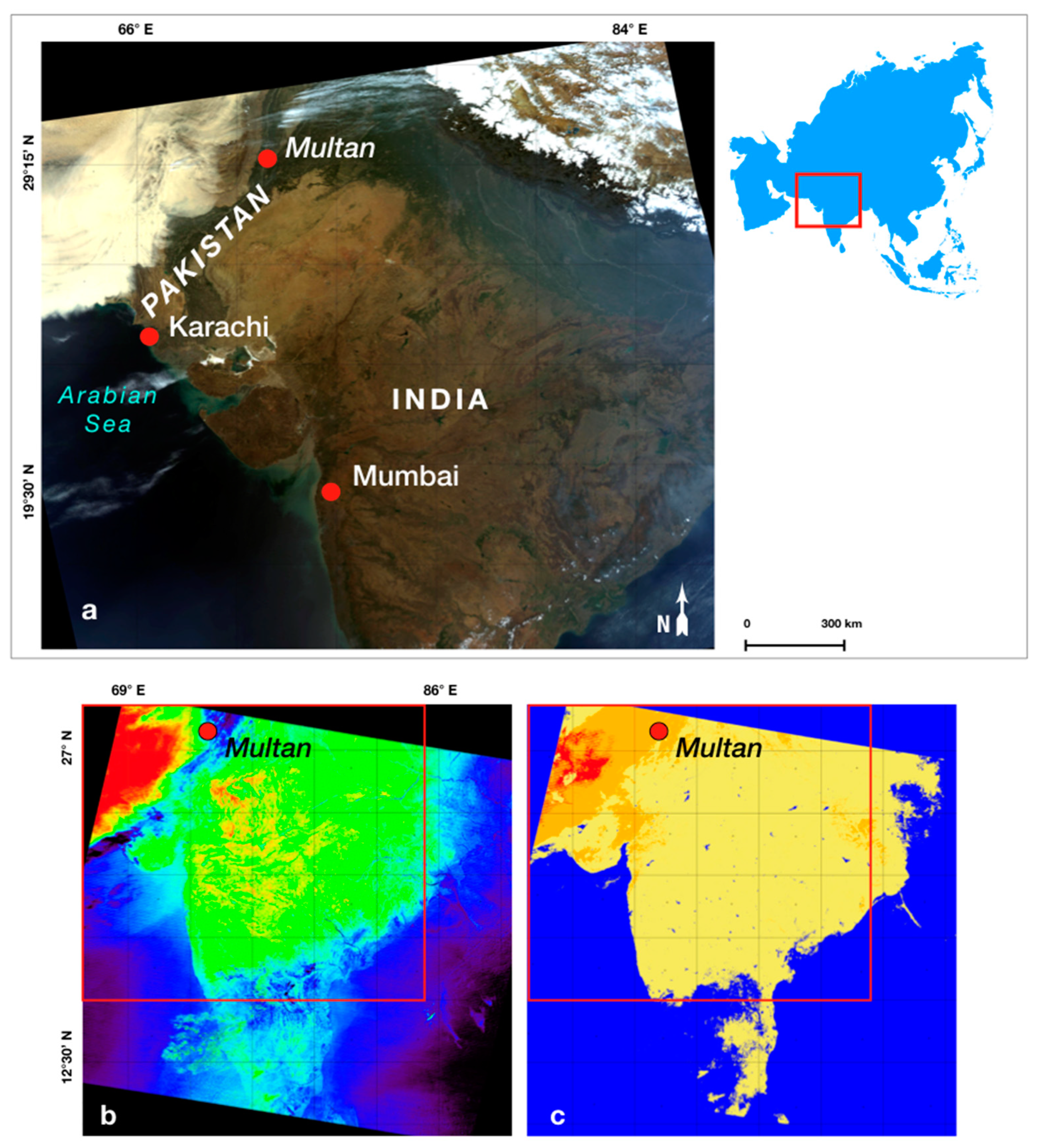
  55. Melis, M.T.; Locci, F.; Dessì, F.; Vuillermoz, E. Dust Storm Monitoring with MODIS Data on the Multan Region (Pakistan); Rendiconti Online Societa Geologica Italiana: Milano, Italy, 2014; Volume 31, p. 2014. [Google Scholar]
  56. Vuillermoz, E.; Cristofanelli, P.; Putero, D.; Verza, G.; Alborighetti, M.; Melis, M.T.; Rasul, G.; Listo, L.; Bonasoni, P. Sustainable Social, Economic and Environmental Revitalization in Multan City. In Sustainable Social, Economic and Environmental Revitalization in Multan City; Research for Development; Springer: Cham, Switzerland, 2014; pp. 137–147. ISBN 978-3-319-02117-1. [Google Scholar]
  57. Kuenzer, C.; Dech, S. Theoretical Background of Thermal Infrared Remote Sensing. In Thermal Infrared Remote Sensing: Sensors, Methods, Applications; Kuenzer, C., Dech, S., Eds.; Springer Netherlands: Dordrecht, The Netherlands, 2013; pp. 1–26. ISBN 978-94-007-6639-6. [Google Scholar]
  58. Prakash, A. Thermal Remote Sensing: Concepts, issues and applications. Int. Arch. Photogramm. Remote Sens. 2000, XXXIII, 239–243. [Google Scholar]
  59. Sabins, F.F.; Ellis, J.M. Remote Sensing: Principles, Interpretation, and Applications, 4th ed.; Waveland Press: Long Grove, IL, USA, 2020; ISBN 978-1-4786-4506-1. [Google Scholar]
  60. Schowengerdt, R. Remote Sensing 2nd Edition Models and Methods for Image Processing; Academic Press: Cambridge, MA, USA, 2012; ISBN 978-0-08-051610-3. [Google Scholar]
  61. Blackett, M. An Overview of Infrared Remote Sensing of Volcanic Activity. J. Imaging 2017, 3, 13. [Google Scholar] [CrossRef]
  62. Oppenheimer, C.; Yirgu, G. Thermal imaging of an active lava lake: Erta ’Ale volcano, Ethiopia. Int. J. Remote Sens. 2002, 23, 4777–4782. [Google Scholar] [CrossRef]
  63. Lagios, E.; Vassilopoulou, S.; Sakkas, V.; Dietrich, V.; Damiata, B.; Ganas, A. Testing satellite and ground thermal imaging of low-temperature fumarolic fields: The dormant Nisyros Volcano (Greece). ISPRS J. Photogramm. Remote Sens. 2007, 62, 447–460. [Google Scholar] [CrossRef]
  64. Spampinato, L.; Calvari, S.; Oppenheimer, C.; Boschi, E. Volcano surveillance using infrared cameras. Earth Sci. Rev. 2011, 106, 63–91. [Google Scholar] [CrossRef]
  65. Pioli, L.; Harris, A.J.L. Real-Time Geophysical Monitoring of Particle Size Distribution during Volcanic Explosions at Stromboli Volcano (Italy). Front. Earth Sci. 2019, 7, 52. [Google Scholar] [CrossRef] [Green Version]
  66. Bombrun, M.; Jessop, D.; Harris, A.; Barra, V. An algorithm for the detection and characterisation of volcanic plumes using thermal camera imagery. J. Volcanol. Geotherm. Res. 2018, 352, 26–37. [Google Scholar] [CrossRef]
  67. Prendes-Gero, M.B.; Suárez-Domínguez, F.J.; González-Nicieza, C.; Álvarez-Fernández, M.I. Infrared Thermography Methodology Applied to Detect Localized Rockfalls in Self-Supporting Underground Mines. In Proceedings of the ISRM-EUROCK-2013-129, Wroclaw, Poland, 23–26 October 2013; International Society for Rock Mechanics and Rock Engineering: Salzburg, Austria, 2013; p. 5. [Google Scholar]
  68. Czajkowski, K.; Goward, S.; Mulhern, T.; Goetz, S.; Walz, A.; Shirey, D.; Stadler, S.; Prince, S.; Dubayah, R.; Quattrochi, D.; et al. Estimating environmental variables using thermal remote sensing. Therm. Remote Sens. Land Surf. Process. 2004, 11–32. [Google Scholar] [CrossRef]
  69. Njoku, E.G. Encyclopedia of Remote Sensing; Encyclopedia of Earth Sciences Series; Springer: New York, NY, USA, 2014; ISBN 978-0-387-36698-2. [Google Scholar]
  70. Gillespie, A.; Rokugawa, S.; Matsunaga, T.; Cothern, J.; Hook, S.; Kahle, A. A temperature and emissivity separation algorithm for Advanced Spaceborne Thermal Emission and Reflection Radiometer (ASTER) images. IEEE Trans. Geosci. Remote Sens. 1998, 36, 1113–1126. [Google Scholar] [CrossRef]
  71. Sobrino, J.A.; Oltra-Carrió, R.; Jiménez-Muñoz, J.C.; Julien, Y.; Soria, G.; Franch, B.; Mattar, C. Emissivity mapping over urban areas using a classification-based approach: Application to the Dual-use European Security IR Experiment (DESIREX). Int. J. Appl. Earth Obs. Geoinf. 2012, 18, 141–147. [Google Scholar] [CrossRef]
  72. Becker, F. The impact of spectral emissivity on the measurement of land surface temperature from a satellite. Int. J. Remote Sens. 1987, 8, 1509–1522. [Google Scholar] [CrossRef]
  73. Nerry, F.; Labed, J.; Stoll, M.P. Spectral properties of land surfaces in the thermal infrared: 1. Laboratory measurements of absolute spectral emissivity signatures. J. Geophys. Res. Space Phys. 1990, 95, 7027. [Google Scholar] [CrossRef]
  74. Hook, S.J.; Gabell, A.; Green, A.; Kealy, P. A comparison of techniques for extracting emissivity information from thermal infrared data for geologic studies. Remote Sens. Environ. 1992, 42, 123–135. [Google Scholar] [CrossRef]
  75. Liang, S.; Wang, J. Land surface temperature and thermal infrared emissivity. In Advanced Remote Sensing: Terrestrial Information Extraction and Applications; Academic Press: Cambridge, MA, USA, 2020; ISBN 978-0-12-816528-7. [Google Scholar]
  76. Taranik, J.V.; Coolbaugh, M.F.; Vaughan, R.G.; Bedell, R.; Crósta, A.P.; Grunsky, E. An Overview of Thermal Infrared Remote Sensing with Applications to Geothermal and Mineral Exploration in the Great Basin, Western United States. Remote Sens. Spectr. Geol. 2009, 16, 41–57. [Google Scholar] [CrossRef]
  77. Tomlinson, C.J.; Chapman, L.; Thornes, J.E.; Baker, C. Remote sensing land surface temperature for meteorology and climatology: A review. Meteorol. Appl. 2011, 18, 296–306. [Google Scholar] [CrossRef] [Green Version]
  78. Rautio, A.B.K.; Korkka-Niemi, K.I.; Salonen, V.-P. Thermal infrared remote sensing in assessing groundwater and surface-water resources related to Hannukainen mining development site, northern Finland. Hydrogeol. J. 2017, 26, 163–183. [Google Scholar] [CrossRef]
  79. Wawrzyniak, V.; Piégay, H.; Allemand, P.; Vaudor, L.; Grandjean, P. Prediction of water temperature heterogeneity of braided rivers using very high resolution thermal infrared (TIR) images. Int. J. Remote Sens. 2013, 34, 4812–4831. [Google Scholar] [CrossRef]
  80. Ishimwe, R.; Abutaleb, K.; Ahmed, F. Applications of Thermal Imaging in Agriculture—A Review. Adv. Remote Sens. 2014, 3, 128–140. [Google Scholar] [CrossRef] [Green Version]
  81. Bejannin, S.; Van Beek, P.; Stieglitz, T.C.; Souhaut, M.; Tamborski, J. Combining airborne thermal infrared images and radium isotopes to study submarine groundwater discharge along the French Mediterranean coastline. J. Hydrol. Reg. Stud. 2017, 13, 72–90. [Google Scholar] [CrossRef]
  82. Antoine, R.; Fauchard, C.; Oehler, J.-F.; Joignant, P. Permeability and voids influence on the thermal signal, as inferred by multitemporal UAV-based infrared and visible images. J. Hydrol. 2020, 587, 124907. [Google Scholar] [CrossRef]
  83. Eisele, A.; Chabrillat, S.; Hecker, C.; Hewson, R.; Lau, I.C.; Rogass, C.; Segl, K.; Cudahy, T.J.; Udelhoven, T.; Hostert, P.; et al. Advantages using the thermal infrared (TIR) to detect and quantify semi-arid soil properties. Remote Sens. Environ. 2015, 163, 296–311. [Google Scholar] [CrossRef]
  84. Rowan, L.; Kahale, A.B. Evaluation of 0.46- to 2.36-mu m Multispectral Scanner Images of the East Tintic Mining District, Utah, for Mapping Hydrothermally Altered Rock. Econ. Geol. 1982, 77, 441–452. [Google Scholar] [CrossRef]
  85. Belward, A.S.; Skøien, J.O. Who launched what, when and why; trends in global land-cover observation capacity from civilian earth observation satellites. ISPRS J. Photogramm. Remote Sens. 2015, 103, 115–128. [Google Scholar] [CrossRef]
  86. Abrams, M.; Yamaguchi, Y. Twenty Years of ASTER Contributions to Lithologic Mapping and Mineral Exploration. Remote Sens. 2019, 11, 1394. [Google Scholar] [CrossRef] [Green Version]
  87. Mushkin, A.; Gillespie, A.R.; Abbott, E.A.; Batbaatar, J.; Hulley, G.; Tan, H.; Tratt, D.M.; Buckland, K.N. Validation of ASTER Emissivity Retrieval Using the Mako Airborne TIR Imaging Spectrometer at the Algodones Dune Field in Southern California, USA. Remote Sens. 2020, 12, 815. [Google Scholar] [CrossRef] [Green Version]
  88. Yousefi, B.; Sojasi, S.; Castanedo, C.I.; Beaudoin, G.; Huot, F.; Maldague, X.P.V.; Chamberland, M.; Lalonde, E. Emissivity retrieval from indoor hyperspectral imaging of mineral grains. In Proceedings of the SPIE, Baltimore, MD, USA, 14 April 2016; Volume 9861. [Google Scholar]
  89. Quattrochi, D.; Luvall, J. Thermal Remote Sensing in Land Surface Processing; CRC Press: Boca Raton, FL, USA, 2004; ISBN 978-0-415-30224-1. [Google Scholar]
  90. Mcgonigle, A.; Aiuppa, A.; Giudice, G.; Tamburello, G.; Hodson, A.J.; Gurrieri, S. Unmanned aerial vehicle measurements of volcanic carbon dioxide fluxes. Geophys. Res. Lett. 2008, 35, 35. [Google Scholar] [CrossRef] [Green Version]
  91. Bonali, F.L.; Tibaldi, A.; Marchese, F.; Fallati, L.; Russo, E.; Corselli, C.; Savini, A. UAV-based surveying in volcano-tectonics: An example from the Iceland rift. J. Struct. Geol. 2019, 121, 46–64. [Google Scholar] [CrossRef]
  92. Sheng, H.; Chao, H.; Coopmans, C.; Han, J.; McKee, M.; Chen, Y. Low-cost UAV-Based Thermal Infrared Remote Sensing: Platform, Calibration and Applications-IEEE Conference Publication. Available online: https://ieeexplore.ieee.org/document/5552031/ (accessed on 13 April 2020).
  93. Rossi, G.; Tanteri, L.; Tofani, V.; Vannocci, P.; Moretti, S.; Casagli, N. Multitemporal UAV surveys for landslide mapping and characterization. Landslides 2018, 15, 1045–1052. [Google Scholar] [CrossRef] [Green Version]
  94. Eisenbeiss, H. UAV Photogrammetry. Ph.D. Thesis, ETH Zurich, Zurich, Switzerland, 2009. [Google Scholar]
  95. Eisenbeiss, H.; Sauerbier, M. Investigation of uav systems and flight modes for photogrammetric applications. Photogramm. Rec. 2011, 26, 400–421. [Google Scholar] [CrossRef]
  96. Nex, F.; Remondino, F. UAV for 3D mapping applications: A review. Appl. Geomat. 2013, 6, 1–15. [Google Scholar] [CrossRef]
  97. Frodella, W.; Elashvili, M.; Spizzichino, D.; Gigli, G.; Adikashvili, L.; Vacheishvili, N.; Kirkitadze, G.; Nadaraia, A.; Margottini, C.; Casagli, N. Combining InfraRed Thermography and UAV Digital Photogrammetry for the Protection and Conservation of Rupestrian Cultural Heritage Sites in Georgia: A Methodological Application. Remote Sens. 2020, 12, 892. [Google Scholar] [CrossRef] [Green Version]
  98. Scaioni, M.; Longoni, L.; Melillo, V.; Papini, M. Remote Sensing for Landslide Investigations: An Overview of Recent Achievements and Perspectives. Remote Sens. 2014, 6, 12666. [Google Scholar] [CrossRef] [Green Version]
  99. Maes, W.; Pashuysen, T.; Trabucco, A.; Veroustraete, F.; Muys, B. Does energy dissipation increase with ecosystem succession? Testing the ecosystem exergy theory combining theoretical simulations and thermal remote sensing observations. Ecol. Model. 2011, 222, 3917–3941. [Google Scholar] [CrossRef]
  100. Maes, W.; Huete, A.; Steppe, K. Optimizing the Processing of UAV-Based Thermal Imagery. Remote Sens. 2017, 9, 476. [Google Scholar] [CrossRef] [Green Version]
  101. Ouyang, X.; Chen, D.M.; Duan, S.-B.; Lei, Y.; Dou, Y.; Hu, G. Validation and Analysis of Long-Term AATSR Land Surface Temperature Product in the Heihe River Basin, China. Remote Sens. 2017, 9, 152. [Google Scholar] [CrossRef] [Green Version]
  102. Frodella, W.; Gigli, G.; Morelli, S.; Lombardi, L.; Casagli, N. Landslide Mapping and Characterization through Infrared Thermography (IRT): Suggestions for a Methodological Approach from Some Case Studies. Remote Sens. 2017, 9, 1281. [Google Scholar] [CrossRef] [Green Version]
  103. Sobrino, J.A.; Caselles, V. Thermal infrared radiance model for interpreting the directional radiometric temperature of a vegetative surface. Remote Sens. Environ. 1990, 33, 193–199. [Google Scholar] [CrossRef]
  104. Cao, B.; Liu, Q.; Du, Y.; Bian, Z.; Gastellu, J.-P.; Trigo, I.F.; Zhan, W.; Yu, Y.; Cheng, J.; Jacob, F.; et al. A review of earth surface thermal radiation directionality observing and modeling: Historical development, current status and perspectives. Remote Sens. Environ. 2019, 232, 111304. [Google Scholar] [CrossRef]
  105. Shannon, H.R.; Sigda, J.M.; Van Dam, R.; Hendrickx, J.M.H.; McLemore, V. Thermal Camera Imaging of Rock Piles at the Questa Molybdenum Mine, Questa, New Mexico. J. Am. Soc. Min. Reclam. 2005, 2005, 1015–1028. [Google Scholar] [CrossRef]
  106. Wu, J.-H.; Lin, H.-M.; Lee, D.-H.; Fang, S.-C. Integrity assessment of rock mass behind the shotcreted slope using thermography. Eng. Geol. 2005, 80, 164–173. [Google Scholar] [CrossRef]
  107. Teza, G.; Marcato, G.; Castelli, E.; Galgaro, A. IRTROCK: A MATLAB toolbox for contactless recognition of surface and shallow weakness of a rock cliff by infrared thermography. Comput. Geosci. 2012, 45, 109–118. [Google Scholar] [CrossRef]
  108. Baroň, I.; Bečkovský, D.; Míča, L. Application of infrared thermography for mapping open fractures in deep-seated rockslides and unstable cliffs. Landslides 2012, 11, 15–27. [Google Scholar] [CrossRef]
  109. Mineo, S.; Pappalardo, G. The Use of Infrared Thermography for Porosity Assessment of Intact Rock. Rock Mech. Rock Eng. 2016, 49, 3027–3039. [Google Scholar] [CrossRef]
  110. Fiorucci, M.; Marmoni, G.M.; Martino, S.; Mazzanti, P. Thermal Response of Jointed Rock Masses Inferred from Infrared Thermographic Surveying (Acuto Test-Site, Italy). Sensors 2018, 18, 2221. [Google Scholar] [CrossRef] [PubMed] [Green Version]
  111. Sagan, V.; Maimaitijiang, M.; Sagan, V.; Eblimit, K.; Peterson, K.; Hartling, S.; Esposito, F.; Khanal, K.; Newcomb, M.; Pauli, D.; et al. UAV-Based High Resolution Thermal Imaging for Vegetation Monitoring, and Plant Phenotyping Using ICI 8640 P, FLIR Vue Pro R 640, and thermoMap Cameras. Remote Sens. 2019, 11, 330. [Google Scholar] [CrossRef] [Green Version]
  112. Lagüela, S.; Díaz-Vilariño, L.; Martínez-Sánchez, J.; Armesto, J. Automatic thermographic and RGB texture of as-built BIM for energy rehabilitation purposes. Autom. Constr. 2013, 31, 230–240. [Google Scholar] [CrossRef]
  113. Pappalardo, G.; Mineo, S.; Zampelli, S.P.; Cubito, A.; Calcaterra, D. InfraRed Thermography proposed for the estimation of the Cooling Rate Index in the remote survey of rock masses. Int. J. Rock Mech. Min. Sci. 2016, 83, 182–196. [Google Scholar] [CrossRef]
  114. Schläpfer, D.; Richter, R. Geo-atmospheric processing of airborne imaging spectrometry data. Part 1: Parametric orthorectification. Int. J. Remote Sens. 2002, 23, 2609–2630. [Google Scholar] [CrossRef]
  115. Jimenez-Berni, J.A.; Zarco-Tejada, P.J.; Suarez, L.; Fereres, E. Thermal and Narrowband Multispectral Remote Sensing for Vegetation Monitoring From an Unmanned Aerial Vehicle. IEEE Trans. Geosci. Remote Sens. 2009, 47, 722–738. [Google Scholar] [CrossRef] [Green Version]
  116. Luhmann, T.; Fraser, C.; Maas, H.-G. Sensor modelling and camera calibration for close-range photogrammetry. ISPRS J. Photogramm. Remote Sens. 2016, 115, 37–46. [Google Scholar] [CrossRef]
  117. Wei, Y.-M.; Kang, L.; Yang, B.; Wu, L.-D. Applications of structure from motion: A survey. J. Zhejiang Univ. Sci. C 2013, 14, 486–494. [Google Scholar] [CrossRef]
  118. James, M.R.; Robson, S.; D’Oleire-Oltmanns, S.; Niethammer, U. Optimising UAV topographic surveys processed with structure-from-motion: Ground control quality, quantity and bundle adjustment. Geomorphology 2017, 280, 51–66. [Google Scholar] [CrossRef] [Green Version]
  119. Jaboyedoff, M. Introduction to Vertical Geology thematic issue. Eur. J. Remote Sens. 2015, 48, 479–487. [Google Scholar] [CrossRef] [Green Version]
  120. Granshaw, S.I. Structure from motion: Origins and originality. Photogramm. Rec. 2018, 33, 6–10. [Google Scholar] [CrossRef]
  121. Scaioni, M.; Crippa, J.; Corti, M.; Barazzetti, L.; Fugazza, D.; Azzoni, R.; Cernuschi, M.; Diolaiuti, G.A. Technical Aspects Related to the Application of SFM Photogrammetry in High Mountain. ISPRS Int. Arch. Photogramm. Remote Sens. Spat. Inf. Sci. 2018, 1029–1036. [Google Scholar] [CrossRef] [Green Version]
  122. Dall’Asta, E.; Forlani, G.; Roncella, R.; Santise, M.; Diotri, F.; Di Cella, U.M. Unmanned Aerial Systems and DSM matching for rock glacier monitoring. ISPRS J. Photogramm. Remote Sens. 2017, 127, 102–114. [Google Scholar] [CrossRef]
  123. Helgesen, H.H.; Leira, F.S.; Bryne, T.H.; Albrektsen, S.M.; Johansen, T.A. Real-time georeferencing of thermal images using small fixed-wing UAVs in maritime environments. ISPRS J. Photogramm. Remote Sens. 2019, 154, 84–97. [Google Scholar] [CrossRef]
  124. Bendig, J.; Yu, K.; Aasen, H.; Bolten, A.; Bennertz, S.; Broscheit, J.; Gnyp, M.L.; Bareth, G. Combining UAV-based plant height from crop surface models, visible, and near infrared vegetation indices for biomass monitoring in barley. Int. J. Appl. Earth Obs. Geoinf. 2015, 39, 79–87. [Google Scholar] [CrossRef]
  125. Shi, Y.; Thomasson, J.A.; Murray, S.C.; Pugh, N.A.; Rooney, W.L.; Shafian, S.; Rajan, N.; Rouze, G.; Morgan, C.L.S.; Neely, H.L.; et al. Unmanned Aerial Vehicles for High-Throughput Phenotyping and Agronomic Research. PLoS ONE 2016, 11, e0159781. [Google Scholar] [CrossRef] [Green Version]
  126. Honkavaara, E.; Eskelinen, M.; Pölönen, I.; Saari, H.; Ojanen, H.; Mannila, R.; Holmlund, C.; Hakala, T.; Litkey, P.; Rosnell, T.; et al. Remote Sensing of 3-D Geometry and Surface Moisture of a Peat Production Area Using Hyperspectral Frame Cameras in Visible to Short-Wave Infrared Spectral Ranges Onboard a Small Unmanned Airborne Vehicle (UAV). IEEE Trans. Geosci. Remote Sens. 2016, 54, 5440–5454. [Google Scholar] [CrossRef] [Green Version]
  127. Conte, P.; Girelli, V.A.; Mandanici, E. Structure from Motion for aerial thermal imagery at city scale: Pre-processing, camera calibration, accuracy assessment. ISPRS J. Photogramm. Remote Sens. 2018, 146, 320–333. [Google Scholar] [CrossRef]
  128. Maset, E.; Fusiello, A.; Crosilla, F.; Toldo, R.; Zorzetto, D. PHOTOGRAMMETRIC 3D BUILDING RECONSTRUCTION FROM THERMAL IMAGES. ISPRS Ann. Photogramm. Remote Sens. Spat. Inf. Sci. 2017, 2, 25–32. [Google Scholar] [CrossRef] [Green Version]
  129. Turner, D.; Lucieer, A.; Malenovsky, Z.; King, D.; Robinson, S.A. Spatial Co-Registration of Ultra-High Resolution Visible, Multispectral and Thermal Images Acquired with a Micro-UAV over Antarctic Moss Beds. Remote Sens. 2014, 6, 4003–4024. [Google Scholar] [CrossRef] [Green Version]
  130. Pérez-García, J.L.; Sánchez-Gómez, M.; Gómez-López, J.M.; Guerra, T.; Gil, D.; Fernández, T. Georeferenced thermal infrared images from UAV surveys as a potential tool to detect and characterize shallow cave ducts. Eng. Geol. 2018, 246, 277–287. [Google Scholar] [CrossRef]
  131. Dillen, M.; Vanhellemont, M.; Verdonckt, P.; Maes, W.; Steppe, K.; Verheyen, K. Productivity, stand dynamics and the selection effect in a mixed willow clone short rotation coppice plantation. Biomass Bioenergy 2016, 87, 46–54. [Google Scholar] [CrossRef]
  132. Hoffmann, H.; Nieto, H.; Jensen, R.; Guzinski, R.; Zarco-Tejada, P.; Friborg, T. Estimating evaporation with thermal UAV data and two-source energy balance models. Hydrol. Earth Syst. Sci. 2016, 20, 697–713. [Google Scholar] [CrossRef] [Green Version]
  133. Pech, K.; Stelling, N.; Karrasch, P.; Maas, H.-G. Generation of Multitemporal Thermal Orthophotos from UAV Data. ISPRS Int. Arch. Photogramm. Remote Sens. Spat. Inf. Sci. 2013, XL-1-W2, 305–310. [Google Scholar] [CrossRef] [Green Version]
  134. Previtali, M.; Barazzetti, L.; Redaelli, V.; Scaioni, M.; Rosina, E. Rigorous procedure for mapping thermal infrared images on three-dimensional models of building façades. J. Appl. Remote Sens. 2013, 7, 73503. [Google Scholar] [CrossRef] [Green Version]
  135. Yahyanejad, S.; Rinner, B. A fast and mobile system for registration of low-altitude visual and thermal aerial images using multiple small-scale UAVs. ISPRS J. Photogramm. Remote Sens. 2015, 104, 189–202. [Google Scholar] [CrossRef]
  136. Hartmann, W.; Tilch, S.; Eisenbeiss, H.; Schindler, K. Determination of the UAV Position by Automatic Processing of Thermal Images. ISPRS Int. Arch. Photogramm. Remote Sens. Spat. Inf. Sci. 2012, 111–116. [Google Scholar] [CrossRef] [Green Version]
  137. Boesch, R. Thermal Remote Sensing with UAV-Based Workflows. ISPRS Int. Arch. Photogramm. Remote Sens. Spat. Inf. Sci. 2017, 41–46. [Google Scholar] [CrossRef] [Green Version]
  138. Ostermann, F. Anwendungstechnologie Aluminium; VDI-Buch; 3, neu bearbeitete Auflage; Springer Vieweg: Berlin, Germany, 2014; ISBN 978-3-662-43807-7. [Google Scholar]
  139. Luhmann, T.; Piechel, J.; Roelfs, T. Geometric Calibration of Thermographic Cameras. In Thermal Infrared Remote Sensing. Remote Sensing and Digital Image Processing; Kuenzer, C., Dech, S., Eds.; Springer: Dordrecht, The Netherlands, 2013; Volume 17, ISBN 978-94-007-6639-6. [Google Scholar]
  140. Matese, A.; Di Gennaro, S.F. Practical Applications of a Multisensor UAV Platform Based on Multispectral, Thermal and RGB High Resolution Images in Precision Viticulture. Agriculture 2018, 8, 116. [Google Scholar] [CrossRef] [Green Version]
  141. Dering, G.M.; Micklethwaite, S.; Thiele, S.T.; Vollgger, S.A.; Cruden, A.R. Review of drones, photogrammetry and emerging sensor technology for the study of dykes: Best practises and future potential. J. Volcanol. Geotherm. Res. 2019, 373, 148–166. [Google Scholar] [CrossRef]
  142. Tucci, G.; Parisi, E.I.; Castelli, G.; Errico, A.; Corongiu, M.; Sona, G.; Viviani, E.; Bresci, E.; Preti, F. Multi-Sensor UAV Application for Thermal Analysis on a Dry-Stone Terraced Vineyard in Rural Tuscany Landscape. ISPRS Int. J. Geo Inf. 2019, 8, 87. [Google Scholar] [CrossRef] [Green Version]
  143. Tewinkel, G.C. Basic mathematics of photogrammetry. In Manual of Photogrammetry; U.S. Department of Commerce, Coast and Geodetic Survey, 1963. [Google Scholar]
  144. Piralilou, S.T.; Shahabi, H.; Jarihani, B.; Ghorbanzadeh, O.; Blaschke, T.; Gholamnia, K.; Meena, S.R.; Aryal, J. Landslide Detection Using Multi-Scale Image Segmentation and Different Machine Learning Models in the Higher Himalayas. Remote Sens. 2019, 11, 2575. [Google Scholar] [CrossRef] [Green Version]
  145. Wolf, P.R.; Dewitt, B.A.; Wilkinson, B.E. Elements of Photogrammetry with Applications in GIS, 4th ed.; McGraw-Hill Education: New York, NY, USA, 2014; ISBN 978-0-07-176112-3. [Google Scholar]
  146. Danzi, M.; Di Crescenzo, G.; Ramondini, M.; Santo, A. Use of Unmanned Aerial Vehicles (Uavs) for Photogrammetric Surveys in Rockfall Instability Studies; Rendiconti Online Societa Geologica Italiana: Milano, Italy, 2013; Volume 23. [Google Scholar]
  147. Ruiz-Carulla, R.; Corominas, J.; Mavrouli, O. A methodology to obtain the block size distribution of fragmental rockfall deposits. Landslides 2015, 12, 815–825. [Google Scholar] [CrossRef] [Green Version]
  148. Mazzanti, P.; Brunetti, A.; Bretschneider, A. A New Approach Based on Terrestrial Remote-sensing Techniques for Rock Fall Hazard Assessment. In Modern Technologies for Landslide Monitoring and Prediction; Scaioni, M., Ed.; Springer Natural Hazards; Springer: Berlin/Heidelberg, Germany, 2015; pp. 69–87. ISBN 978-3-662-45931-7. [Google Scholar]
  149. Iwaszczuk, D.; Stilla, U. Camera pose refinement by matching uncertain 3D building models with thermal infrared image sequences for high quality texture extraction. ISPRS J. Photogramm. Remote Sens. 2017, 132, 33–47. [Google Scholar] [CrossRef]
  150. Lin, D.; Jarzabek-Rychard, M.; Tong, X.; Maas, H.-G. Fusion of thermal imagery with point clouds for building façade thermal attribute mapping. ISPRS J. Photogramm. Remote Sens. 2019, 151, 162–175. [Google Scholar] [CrossRef]
  151. Alba, M.I.; Barazzetti, L.; Scaioni, M.; Rosina, E.; Previtali, M. Mapping Infrared Data on Terrestrial Laser Scanning 3D Models of Buildings. Remote Sens. 2011, 3, 1847–1870. [Google Scholar] [CrossRef] [Green Version]
  152. Chapter 7-Land surface temperature and thermal infrared emissivity. In Advanced Remote Sensing, 2nd ed.; Liang, S.; Wang, J. (Eds.) Academic Press: Cambridge, MA, USA, 2020; pp. 251–295. ISBN 978-0-12-815826-5. [Google Scholar]
  153. Mineo, S.; Pappalardo, G.; Rapisarda, F.; Cubito, A.; Di Maria, G. Integrated geostructural, seismic and infrared thermography surveys for the study of an unstable rock slope in the Peloritani Chain (NE Sicily). Eng. Geol. 2015, 195, 225–235. [Google Scholar] [CrossRef]
  154. Zaragoza, I.M.-E.; Caroti, G.; Piemonte, A.; Riedel, B.; Tengen, D.; Niemeier, W. Structure from motion (SfM) processing of UAV images and combination with terrestrial laser scanning, applied for a 3D-documentation in a hazardous situation. Geomat. Nat. Hazards Risk 2017, 8, 1492–1504. [Google Scholar] [CrossRef]
  155. Liu, S.; Wu, L.; Ma, B. Infrared Imaging Detection of Hidden Danger in Mine Engineering. In Proceedings of the PIERS, Suzhou, China, 12–16 September 2011. [Google Scholar]
  156. Squarzoni, C.; Galgaro, A.; Teza, G.; Acosta, C.A.T.; Pernito, M.A.; Bucceri, N. Terrestrial laser scanner and infrared thermography in rock fall prone slope analysis. Geophys. Res. Abstr. 2008, 10. EGU2008-A-09254. [Google Scholar]
  157. Baroň, I.; Bečkovský, D. Infrared Thermographic Survey of Pseudokarst Sites in The Fysch Belt Of Outer West Carpathians (Czech Republic). In Proceedings of the 16th International Congress of Speleology, Brno, Czech Republic, 21–28 July 2013; Michal, F., Pavel, B., Eds.; 2013. [Google Scholar]
  158. Mineo, S.; Calcaterra, D.; Zampelli, S.P.; Pappalardo, G. Application of Infrared Thermography for the survey of intensely jointed rock slopes. Rend. Online Soc. Geol. Ital. 2015, 35, 212–215. [Google Scholar] [CrossRef]
  159. Pappalardo, G.; Mineo, S.; Angrisani, A.C.; Di Martire, D.; Calcaterra, D. Combining field data with infrared thermography and DInSAR surveys to evaluate the activity of landslides: The case study of Randazzo Landslide (NE Sicily). Landslides 2018, 15, 2173–2193. [Google Scholar] [CrossRef]
  160. Chicco, J.; Vacha, D.; Mandrone, G. Thermo-Physical and Geo-Mechanical Characterization of Faulted Carbonate Rock Masses (Valdieri, Italy). Remote Sens. 2019, 11, 179. [Google Scholar] [CrossRef] [Green Version]
  161. Barton, N. Suggested methods for the quantitative description of discontinuities in rock masses: International Society for Rock Mechanics. Int. J. Rock Mech. Min. Sci. Geomech. Abstr. 1978, 15, 319–368. [Google Scholar]
  162. Priest, S.D. Discontinuity Analysis for Rock Engineering; Springer Netherlands: Dordrecht, The Netherlands, 1993. [Google Scholar]
  163. Akgun, A.; Sezer, E.A.; Nefeslioglu, H.; Gokceoglu, C.; Pradhan, B. An easy-to-use MATLAB program (MamLand) for the assessment of landslide susceptibility using a Mamdani fuzzy algorithm. Comput. Geosci. 2012, 38, 23–34. [Google Scholar] [CrossRef]
  164. Jaboyedoff, M.; Jaboyedoff, M.; Collins, B.D.; Derron, M.-H.; Stock, G.M.; Matasci, B.; Boesiger, M.; Lefeuvre, C.; Podladchikov, Y.Y. Detection of rock bridges by infrared thermal imaging and modeling. Sci. Rep. 2019, 9, 13138–13219. [Google Scholar] [CrossRef] [Green Version]
  165. Pappalardo, G.; Mineo, S. Study of Jointed and Weathered Rock Slopes through the Innovative Approach of InfraRed Thermography. In Landslides: Theory, Practice and Modelling; Pradhan, S.P., Vishal, V., Singh, T.N., Eds.; Advances in Natural and Technological Hazards Research; Springer International Publishing: Cham, Switzerland, 2019; pp. 85–103. [Google Scholar]
  166. Subramanian, S.S.; Fan, X.; Yunus, A.P.; Van Asch, T.; Scaringi, G.; Xu, Q.; Dai, L.; Ishikawa, T.; Huang, R. A Sequentially Coupled Catchment-Scale Numerical Model for Snowmelt-Induced Soil Slope Instabilities. J. Geophys. Res. Earth Surf. 2020, 125. [Google Scholar] [CrossRef]
  167. Kurylyk, B.L.; MacQuarrie, K.T.; McKenzie, J.M. Climate change impacts on groundwater and soil temperatures in cold and temperate regions: Implications, mathematical theory, and emerging simulation tools. Earth Sci. Rev. 2014, 138, 313–334. [Google Scholar] [CrossRef]
  168. Oni, S.K.; Mieres, F.; Futter, M.N.; Laudon, H. Soil temperature responses to climate change along a gradient of upland–riparian transect in boreal forest. Clim. Chang. 2017, 70, 39–41. [Google Scholar] [CrossRef] [Green Version]
  169. Shibasaki, T.; Matsuura, S.; Okamoto, T. Experimental evidence for shallow, slow-moving landslides activated by a decrease in ground temperature. Geophys. Res. Lett. 2016, 43, 6975–6984. [Google Scholar] [CrossRef]
  170. Shibasaki, T.; Matsuura, S.; Hasegawa, Y. Temperature-dependent residual shear strength characteristics of smectite-bearing landslide soils. J. Geophys. Res. Solid Earth 2017, 122, 1449–1469. [Google Scholar] [CrossRef]
  171. Romero, E.; Villar, M.V.; Lloret, A. Thermo-hydro-mechanical behaviour of two heavily overconsolidated clays. Eng. Geol. 2005, 81, 255–268. [Google Scholar] [CrossRef]
  172. Mašín, D. Coupled Thermohydromechanical Double-Structure Model for Expansive Soils. J. Eng. Mech. 2017, 143, 04017067. [Google Scholar] [CrossRef]
  173. Sun, H.; Mašín, D.; Najser, J.; Scaringi, G. Water retention of a bentonite for deep geological radioactive waste repositories: High-temperature experiments and thermodynamic modeling. Eng. Geol. 2020, 269, 105549. [Google Scholar] [CrossRef]
  174. Villar, M.V.; Lloret, A. Influence of temperature on the hydro-mechanical behaviour of a compacted bentonite. Appl. Clay Sci. 2004, 26, 337–350. [Google Scholar] [CrossRef]
  175. McCartney, J.S.; Jafari, N.H.; Hueckel, T.; Sánchez, M.; Vahedifard, F. Emerging Thermal Issues in Geotechnical Engineering. In Geotechnical Fundamentals for Addressing New World Challenges; Lu, N., Mitchell, J.K., Eds.; Springer International Publishing: Cham, Switzerland, 2019; pp. 275–317. ISBN 978-3-030-06249-1. [Google Scholar]
  176. De Blasio, F.V.; Mazzanti, P. Subaerial and subaqueous dynamics of coastal rockfalls. Geomorphology 2010, 115, 188–193. [Google Scholar] [CrossRef]
  177. Salvini, R.; Francioni, M.; Riccucci, S.; Fantozzi, P.L.; Bonciani, F.; Mancini, S. Stability analysis of “Grotta delle Felci” Cliff (Capri Island, Italy): Structural, engineering–geological, photogrammetric surveys and laser scanning. Bull. Int. Assoc. Eng. Geol. 2011, 70, 549–557. [Google Scholar] [CrossRef]
  178. Sunamura, T. A Relationship between Wave-Induced Cliff Erosion and Erosive Force of Waves. J. Geol. 1977, 85, 613–618. [Google Scholar] [CrossRef]
  179. Andriani, G.F.; Walsh, N. Rocky coast geomorphology and erosional processes: A case study along the Murgia coastline South of Bari, Apulia—SE Italy. Geomorphology 2007, 87, 224–238. [Google Scholar] [CrossRef]
  180. Emery, K.O.; Kuhn, G.G. Sea cliffs: Their processes, profiles, and classification. GSA Bull. 1982, 93, 644. [Google Scholar] [CrossRef]
  181. Hungr, O.; Leroueil, S.; Picarelli, L. The Varnes classification of landslide types, an update. Landslides 2013, 11, 167–194. [Google Scholar] [CrossRef]
  182. Sunamura, T. Rocky coast processes: With special reference to the recession of soft rock cliffs. Proc. Jpn. Acad. Ser. B 2015, 91, 481–500. [Google Scholar] [CrossRef] [PubMed] [Green Version]
  183. Budetta, P.; Galietta, G.; Santo, A. A methodology for the study of the relation between coastal cliff erosion and the mechanical strength of soils and rock masses. Eng. Geol. 2000, 56, 243–256. [Google Scholar] [CrossRef]
  184. De Vita, P.; Cevasco, A.; Cavallo, C. Detailed rock failure susceptibility mapping in steep rocky coasts by means of non-contact geostructural surveys: The case study of the Tigullio Gulf (Eastern Liguria, Northern Italy). Nat. Hazards Earth Syst. Sci. 2012, 12, 867–880. [Google Scholar] [CrossRef] [Green Version]
  185. Budetta, P.; Nappi, M. Heterogeneous rock mass classification by means of the geological strength index: The San Mauro formation (Cilento, Italy). Bull. Int. Assoc. Eng. Geol. 2011, 70, 585–593. [Google Scholar] [CrossRef]
  186. Ružić, I.; Benac, Č.; Marović, I.; Ilic, S. A stability assessment of coastal cliffs using digital imagery. Acta Geotech. Slov. 2015, 12, 25–35. [Google Scholar]
  187. Budetta, P.; De Luca, C. Wedge failure hazard assessment by means of a probabilistic approach for an unstable sea-cliff. Nat. Hazards 2014, 76, 1219–1239. [Google Scholar] [CrossRef]
  188. Budetta, P.; De Luca, C.; Nappi, M. Quantitative rockfall risk assessment for an important road by means of the rockfall risk management (RO.MA.) method. Bull. Int. Assoc. Eng. Geol. 2015, 75, 1377–1397. [Google Scholar] [CrossRef]
  189. Sunamura, T. The Geomorphology of Rocky Coasts; Wiley: Chichester, UK, 1992; ISBN 0-471-91775-3. [Google Scholar]
  190. Martino, S.; Mazzanti, P. Integrating geomechanical surveys and remote sensing for sea cliff slope stability analysis: The Mt. Pucci case study (Italy). Nat. Hazards Earth Syst. Sci. 2014, 14, 831–848. [Google Scholar] [CrossRef] [Green Version]
  191. Winter, M.G.; Smith, J.T.; Fotopoulou, S.; Pitilakis, K.; Mavrouli, O.; Corominas, J.; Argyroudis, S.A. An expert judgement approach to determining the physical vulnerability of roads to debris flow. Bull. Int. Assoc. Eng. Geol. 2014, 73, 291–305. [Google Scholar] [CrossRef]
  192. Aicardi, I.; Chiabrando, F.; Lingua, A.; Noardo, F.; Piras, M.; Vigna, G.B. A methodology for acquisition and processing of thermal data acquired by UAVs: A test about subfluvial springs’ investigations. Geomat. Nat. Hazards Risk 2016, 8, 5–17. [Google Scholar] [CrossRef] [Green Version]
  193. Esposito, G.; Salvini, R.; Matano, F.; Sacchi, M.; Danzi, M.; Somma, R.; Troise, C. Multitemporal monitoring of a coastal landslide through SfM-derived point cloud comparison. Photogramm. Rec. 2017, 32, 459–479. [Google Scholar] [CrossRef] [Green Version]
  194. Harvey, M.; Rowland, J.; Luketina, K. Drone with thermal infrared camera provides high resolution georeferenced imagery of the Waikite geothermal area, New Zealand. J. Volcanol. Geotherm. Res. 2016, 325, 61–69. [Google Scholar] [CrossRef]
  195. Quattrochi, D.A.; Ridd, M.K. Analysis of vegetation within a semi-arid urban environment using high spatial resolution airborne thermal infrared remote sensing data. Atmos. Environ. 1998, 32, 19–33. [Google Scholar] [CrossRef]
  196. Ninomiya, Y.; Fu, B.; Cudahy, T. Detecting lithology with Advanced Spaceborne Thermal Emission and Reflection Radiometer (ASTER) multispectral thermal infrared “radiance-at-sensor” data. Remote Sens. Environ. 2005, 99, 127–139. [Google Scholar] [CrossRef]
  197. Pappalardo, G.; Mineo, S. Investigation on the mechanical attitude of basaltic rocks from Mount Etna through InfraRed Thermography and laboratory tests. Constr. Build. Mater. 2017, 134, 228–235. [Google Scholar] [CrossRef]
  198. Grechi, G.; Marino, S. Preliminary results from Multitemporal Infrared Thermography Surveys at the Wied-Il-Mielah Rock Arch (Island of Gozo). Ital. J. Eng. Geol. Environ. 2019. [Google Scholar] [CrossRef]
Figure 1. Number and year of publication of documents matching the keywords “infrared thermography AND landslide OR rockfall” in Scopus, Web of Science and Google Scholar databases.
Remotesensing 12 01971 g001
Figure 2. Moderate resolution imaging spectroradiometer (MODIS) data acquired during a dust storm in the Punjab province of Pakistan, along the boundary with India: (a) RGB optical data acquired daytime on 19/03/2011; (b) brightness temperature difference applied on nighttime imagery acquired on 19/03/2011 at 20:30 h; (c) classification of the image in b: in red, the relatively strong dust zone, in orange, the relatively weak dust zone, in yellow, the land and in blue, the sea and the clouds [55]. The red box in (b,c) represents the boundary of (a).
Remotesensing 12 01971 g002
Figure 3. Relationship between the spectral radiant emission and the temperature of emitting surfaces according to the wavelength. The Plank function and both the Stefan–Boltzmann and Wien displacement laws are represented. The portions of the spectrum are depicted (modified from [61]).
Remotesensing 12 01971 g003
Figure 4. Paths of electromagnetic radiation: the relative size of the arrows indicates the proportion of energy transferred (modified from [114]).
Remotesensing 12 01971 g004
Figure 5. Coastal cliff near Villaggio Nurra, Sassari, northwest Sardinia, Italy. (A) Optical data and (B) thermal data of the area in the dotted red box. The thermogram was acquired on 3 August 2019 at 18:00 h, including surface temperature profiles (°C). Technical specifications: DJI Zenmuse XT2, Dual 4K, 12MP, 1/1.7″ active-pixel (CMOS) visual sensor and forward looking infrared (FLIR) Tau 2 thermal sensor (resolution 640 × 512 pixels) lens 9 mm; UAV DJI Matrice 200; thermal sensitivity of <50 mK. The cliff is mainly made by: (a) Paleozoic low-grade metamorphites (gray rocks in the left half of the picture) with a pervasive cleavage; (b) Quaternary cross-stratified aeolian sandstones (light brown color in the down left side of the picture) that unconformable rest on the metamorphites; (c) a meter-thick, coarse slope talus (dark brown deposit in the central high side of the picture). Rockfall and toppling mainly affected the metamorphites, but the aeolian sandstones were also affected. High T pixels identify the less coherent rock mass, easily identifying the landslide body. Some low T pixels inside the landslides body point out the occurrence of large blocks. In the still not collapsed metamorphites, high T pixels highlight fractures parallel to the metamorphic cleavage.
Remotesensing 12 01971 g005
Figure 6. Synthesis of the three main steps to produce the final infrared thermographs (IRTs).
Remotesensing 12 01971 g006
Table 1. Primary spectral regions used in remote sensing. The boundaries can vary [60].
NameWavelength Range (μm)Radiation SourceSurface Property of Interest
Visible (V)0.4–0.7solarreflectance
Near infrared (NIR)0.7–1.1solarreflectance
Short wave infrared (SWIR)1.1–1.35
1.4–1.8
2–2.5
solarreflectance
Mid wave infrared (MWIR)3–4
4.5–5
solar, thermalreflectance, temperature
Thermal infrared (TIR)8–9.5
10–14
thermalreflectance, temperature
Microwave, radar1 mm–1 mthermal (passive),
artificial (active)
temperature (passive),
roughness (active)
Table 2. Thermal infrared (TIR) advanced spaceborne thermal emission and reflection radiometer (ASTER) bands with ground sample distance of 90 m.
BandSpectral Range
108.125–8.475 μm
118.475–8.825 μm
128.925–9.275 μm
1310.25–10.95 μm
1410.95–11.65 μm
Table 3. Specifications of thermal cameras utilized in landslide studies cited in this study.
Thermal Cameras/ParametersFLIR SC 3000Therm Tracer Th1101FLIR P640FLIR B360FLIR B335FLIR i7FLIR SC620TESTO 885
Spectral Range (μm)8–98–137,5–137.5–137.5–137.5–137.5–137.5–14
Frame Rate (Hz)50/6030309–303033
Accuracy (+/− °C)1222222
Data FormatIMG, BMPJPEGJPEGJPEGJPEGJPEGBMP, JPEG, PNG
Sensor Resolution (dpi)320 × 240640 × 480320 × 240320 × 240120 × 120640 × 480640 × 480
Radiometric Resolution (bit)8–14141414
Thermal Sensitivity (Noise Equivalent Temperature Difference-NETD) (m K)20506060501004030
Focusautoabsent
Focal Length (mm)818
Weight (g)3200170088088034019001570
IFOV (mrad)1.12.20.651.42.593.71.31.7
Publication[105][106][107][108] [109][97,110][111]
Table 4. Comparison among different survey methods for coastal cliffs prone to landslides.
PHASESConstraintsTraditional Field SurveyTLSPhotogrammetryIRT
PlanningCost-EffectivenessLow costHigh costLow costLow cost [102]
Data ResolutionHigh resolution
(linear data)
Very high resolution
(3D-spatial data)
High resolution
(2D/3D-spatial data)
Medium/high resolution depending on object-sensor distance [110]
Solar IlluminationNo influenceNo influenceHighly dependentStrongly dependent
PortabilityHigh portabilityMedium/Low portabilityHigh portabilityHigh portability [106]
MonitoringQuite impossiblePossible, but with high costs and timePossible and fastPossible and fast
Expected ResultsLocal fractures network3D-fractures network
(Orientation)
3D-fractures network (Orientation)Behavior of the fractures [168]
Data CollectionTime-consuming for data acquisitionHigh time-consuming for wide areasVery slow acquisitionFast acquisitionFast acquisition [106]
Accessibility
(Distance Object-Sensor)
Issues to reach inaccessible areasA ground station is necessaryCapable of reaching inaccessible areasCapable of reaching inaccessible areas
Weather ConditionsPartially limitedCompletely limitedPartially or completely limitedPartially or completely limited [114]
VisibilityDaytimeDaytimeDaytimeDaytime and nighttime [107,114]
Field of ViewLimitedPotential occlusionsCompleteComplete
Data analysis and ResultsGeomechanical FeaturesExpert judgment, maps [194]Fracture network (roughness, orientation, opening).
Point Cloud
Fracture network (roughness, direction, opening).
Ortophotos and Point cloud
Classified fracture network, RQD correlation [168]
Thermal images
Physical PropertiesLimited areas of samplingNoneNoneRelationships between thermal data and porosity and bulk density [109]
Table 5. Main topics covered in the literature and holding device used for the thermal infrared (TIR) camera.
Holding DeviceTopic
Quattrochi et al., 1998
[195]
AirborneThermal energy fluxes of different vegetation types in urban environment
Ninomiya et al., 2005
[196]
SpaceborneDetecting mineralogic or chemical composition of rocks
Wu et al., 2005
[106]
TerrestrialEroded caves inside a shotcreted slope
Sheng et al., 2010AirborneAgriculture field coverage, black marker detection
Teza et al., 2012
[107]
Terrestrial (120–150 m)Shallow inhomogeneities, weathered rock cliff areas
Martino and Mazzanti, 2014
[193]
TerrestrialMain joints, recent collapsed areas/detachments in a rock coastal cliff
Baroň et al., 2014
[108]
Terrestrial and UAVOpen cracks and zones of tension within rock slope instability, loosened rock zones, pseudo-karst caverns
Mineo et al., 2015a;
Pappalardo et al., 2016
[154,165]
Terrestrial (3 m)Geostructural features, fracturing degree, daytime temperature exchange of a rock slope
Mineo et al., 2015b
[160]
TerrestrialThermal contrast between vegetated portion, weathered and bare rock along an unstable slope
Pappalardo et al., 2017
[197]
TerrestrialDiscontinuity system and fracture sectors of a rock wedge
Frodella et al., 2017
[102]
Terrestrial and airborneWedge fractures, erosional channels, scarps, earth flow ponds, seepage sectors, debris cones
Fiorucci et al., 2018
[111]
TerrestrialSurficial temperature distribution on rock
masses—thermal response of jointed rock-block—seasonal behavior differences
Pappalardo et al., 2018
[161]
TerrestrialMorphologic features, lithological differences, Landslides bodies
Grechi and Martino 2019
[198]
Terrestrial (20 m)Surficial temperature distribution of rock mass arch in terms of temporal and spatial evolution
Frodella et al., 2020
[97]
Terrestrial (600 m)Weathering rock areas: Moisture
content connected to the ephemeral drainage network

