Mapping of Snow Depth by Blending Satellite and In-Situ Data Using Two-Dimensional Optimal Interpolation—Application to AMSR2


Abstract
:
1. Introduction
2. Data
2.1. Satellite Snow Data
2.2. In-Situ Snow Data
2.3. Forecast Data
2.4. Ancillary Data
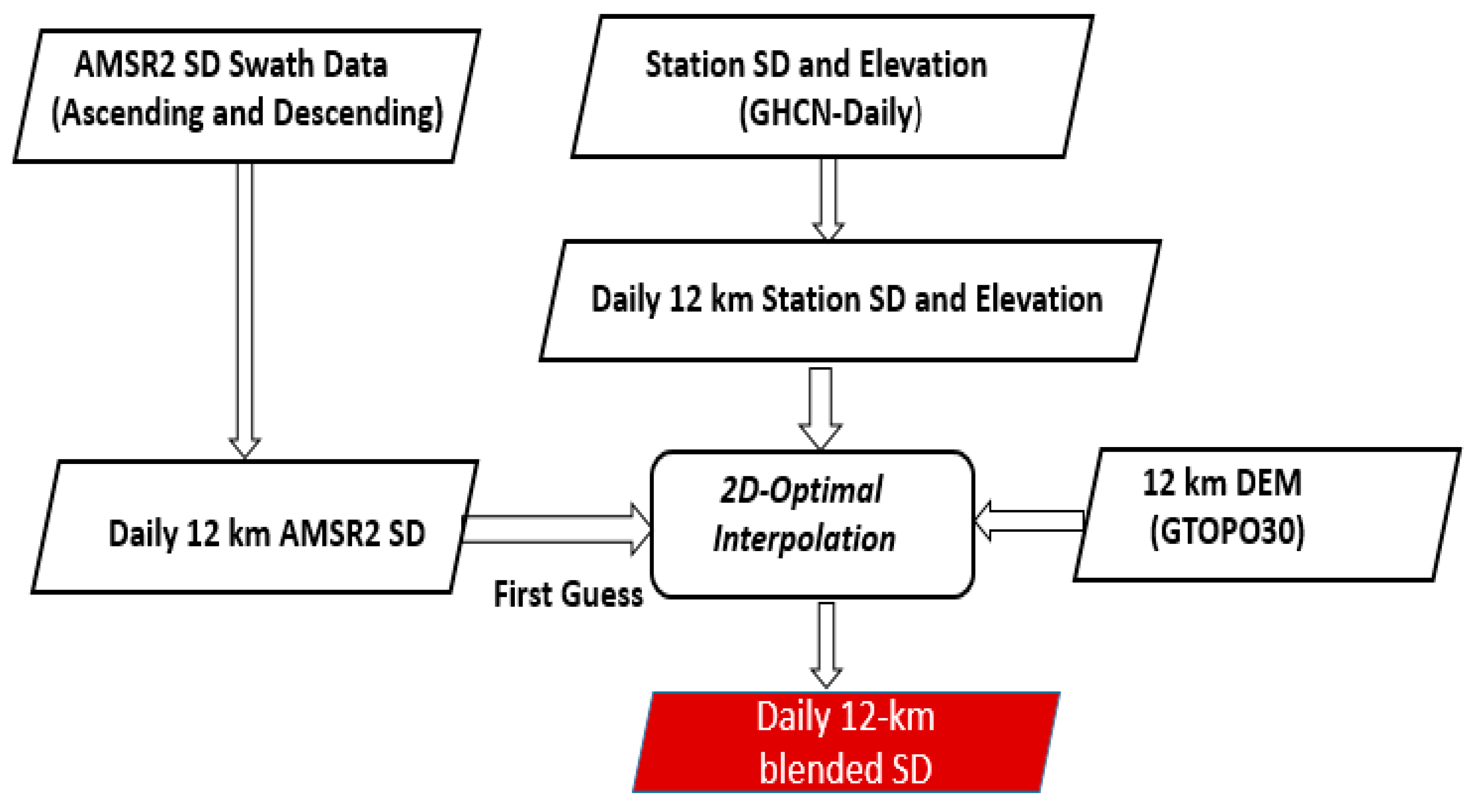
3. Methods
3.1. Two-Dimensional Optimal Interpolation
3.2. Blended Snow Depth Scheme and its Application
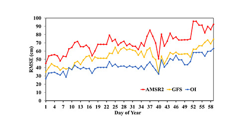
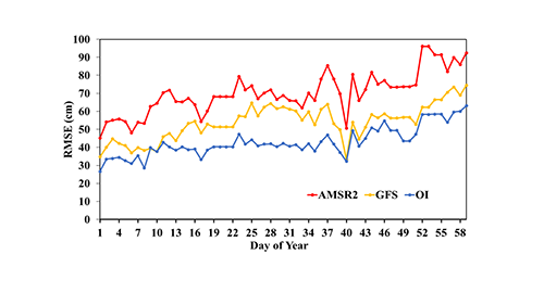
3.3. Evaluation Methodology
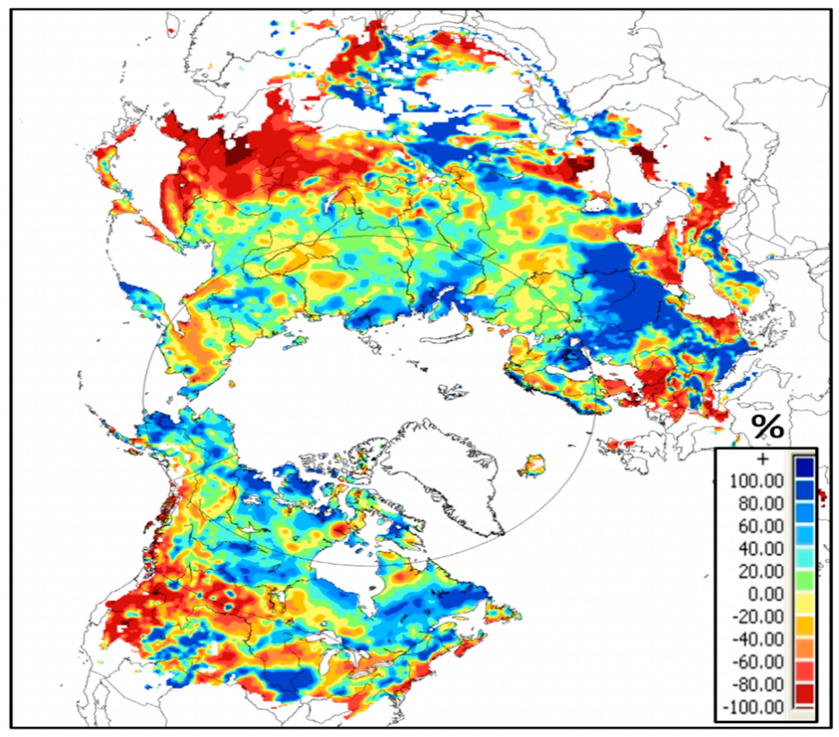
4. Results and Discussion
5. Conclusions
Author Contributions
Funding
Acknowledgments
Conflicts of Interest
References
- Sturm, M.; Taras, B.; Liston, G.E.; Dirksen, C.; Jonas, T.; Leas, J. Estimating Snow Water Equivalent Using Snow Depth Data and Climate Classes. J. Hydrometeorol. 2010, 11, 1380–1394. [Google Scholar] [CrossRef]
- Chang, A.; Foster, J.; Hall, D. Nimbus-7 SMMR derived global snow cover parameters. Ann. Glaciol. 1987, 9, 39–44. [Google Scholar] [CrossRef] [Green Version]
- Goodison, B.E. Determination of areal snow water equivalent on the Canadian prairies using passive microwave satellite data. In Proceedings of the 12th Canadian Symposium on Remote Sensing Geoscience and Remote Sensing Symposium, Vancouver, BC, Canada, 10–14 July 1989; Volume 3, pp. 1243–1246. [Google Scholar]
- Kelly, R.E.; Chang, A.T.; Tsang, L.; Foster, J.L. A prototype AMSR-E global snow area snow depth algorithm. IEEE Trans. Geosci. Remote Sens. 2003, 41, 230–242. [Google Scholar] [CrossRef] [Green Version]
- Kongoli, C.; Grody, N.C.; Ferraro, R.R. Interpretation of AMSU measurements for the retrievals of snow water equivalent and snow depth. J. Geophys. Res. 2004, 109, D24111. [Google Scholar] [CrossRef]
- Kelly, R.E. The AMSR-E Snow Depth Algorithm Description and Initial Results. J. Remote Sens. Soc. Jpn. 2009, 29, 307–317. [Google Scholar]
- Brogioni, M.; Macelloni, G.; Paloscia, S.; Pampaloni, P.; Pettinato, S.; Santi, E.; Xiong, C.; Crepaz, A. Sensitivity analysis of microwave backscattering and emission to snow water equivalent: Synergy of dual sensor observations. In Proceedings of the XXXth URSI General Assembly and Scientific Symposium, Istanbul, Turkey, 13–20 August 2011; pp. 1–3. [Google Scholar]
- Deems, J.S.; Painther, T.H.; Finnegan, D.C. LIDAR measurement of snow depth—A review. J. Glaciol. 2013, 59, 467–479. [Google Scholar] [CrossRef] [Green Version]
- Pulliainen, J.; Grandell, J.; Hallikainen, M.T. HUT snow emission model and its applicability to snow water equivalent retrieval. IEEE Trans. Geosci. Remote Sens. 1999, 37, 1378–1390. [Google Scholar] [CrossRef]
- Pulliainen, J. Mapping of snow water equivalent and snow depth in boreal and sub-arctic zones by assimilating space-borne microwave radiometer data and ground-based observations. Remote Sens. Environ. 2006, 101, 257–269. [Google Scholar] [CrossRef]
- Takala, M.; Luojus, K.; Pulliainen, J.; Derksen, C.; Lemmetyinen, J.; Kärnä, J.-P.; Koskinen, J.; Bojkov, B. Estimating northern hemisphere snow water equivalent for climate research through assimilation of spaceborne radiometer data and ground-based measurements. Remote Sens. Environ. 2011, 115, 3517–3529. [Google Scholar] [CrossRef]
- Grody, N. Relationship between snow parameters and microwave satellite measurements: Theory compared withAdvanced Microwave Sounding Unit observations from 23 to 150 GHz. J. Geophys. Res. 2008, 113, D22108. [Google Scholar] [CrossRef]
- Brasnett, B. A global analysis of snow depth for numerical weather prediction. J. Appl. Meteorol. 1999, 38, 726–740. [Google Scholar] [CrossRef]
- Liu, Y.; Peters-Lidard, C.D.; Kumar, S.; Foster, J.L.; Shaw, M.; Tian, Y.; Fall, G.M. Assimilating satellite-based snow depth and snow cover products for improving snow predictions in Alaska. Adv. Water Resour. 2013, 54, 208–227. [Google Scholar] [CrossRef]
- Liu, Y.; Peters-Lidard, C.D.; Kumar, S.V.; Arsenault, K.R.; Mocko, D.M. Blending satellite-based snow depth products with in situ observations for streamflow predictions in the upper Colorado River Basin. Water Resour. Res. 2015, 51, 1182–1202. [Google Scholar] [CrossRef]
- Grody, N.C. Classification of snow cover and precipitation using the Special Sensor Microwave Imager. J. Geophys. Res. 1991, 96, 7423–7435. [Google Scholar] [CrossRef]
- Grody, N.C.; Basist, A.N. Global identification of snowcover using SSM/I measurements. IEEE Trans. Geosci. Remote Sens. 1996, 34, 237–249. [Google Scholar] [CrossRef]
- Lee, Y.-K.; Kongoli, C.; Key, J. An in-depth evaluation of NOAA’s snow heritage algorithms for snow cover and snow depth using AMSR-E and AMSR2 measurements. J. Atmos. Ocean. Technol. 2015, 32, 2319–2336. [Google Scholar] [CrossRef]
- EMC. The GFS Atmospheric Model; NOAA/NWS/NCEP, NCEP Office Note 442; 2003; p. 14. Available online: http://www.lib.ncep.noaa.gov/ncepofficenotes/files/on442.pdf (accessed on 20 November 2019).
- Ek, M.B.; Mitchell, K.E.; Lin, Y.; Rogers, E.; Grunmann, P.; Koren, V.; Gayno, G.; Tarpley, J.D. Implementation of Noah land surface model advances in the National Centers for Environmental Prediction operational mesoscale Eta model. J. Geophys. Res. 2003, 108, 8851. [Google Scholar] [CrossRef]
- Daley, R. Atmospheric Data Analysis; Cambridge University Press: Cambridge, UK, 1991; p. 457. [Google Scholar]
- de Rosnay, P.; Balsamo, G.; Albergel, C.; Muñoz-Sabater, J.; Isaksen, L. Initialisation of Land Surface Variables for Numerical Weather Prediction. Surv. Geophys. 2012, 35, 607–621. [Google Scholar] [CrossRef]
- Kusabiraki, H. Offline validation of a multi-layer snow scheme for a new land surface model in the operational regional NWP model at JMA. In Proceedings of the 13th EMS Annual Meeting and 11th European Conference on Applications of Meteorology, Reading, UK, 13 September 2013. [Google Scholar]
- Kusabiraki, H. Improvement of Snow Analysis Using an Offline Land-Surface Model. JSC/CAS Working Group on Numerical Experimentation (WGNE). Research Activities in Oceanic and Atmospheric Modelling; Blue Book; World Meteorological Organization (WMO): Geneva, Switzerland, 2015; pp. 1–13. [Google Scholar]
- Helfrich, S.R.; McNamara, D.; Ramsay, B.H.; Baldwin, T.; Kasheta, T. Enhancements to and Forthcoming Developments to the Interactive Multisensor Snow and Ice Mapping System (IMS). Hydrol. Process. 2007, 21, 1576–1586. [Google Scholar] [CrossRef]


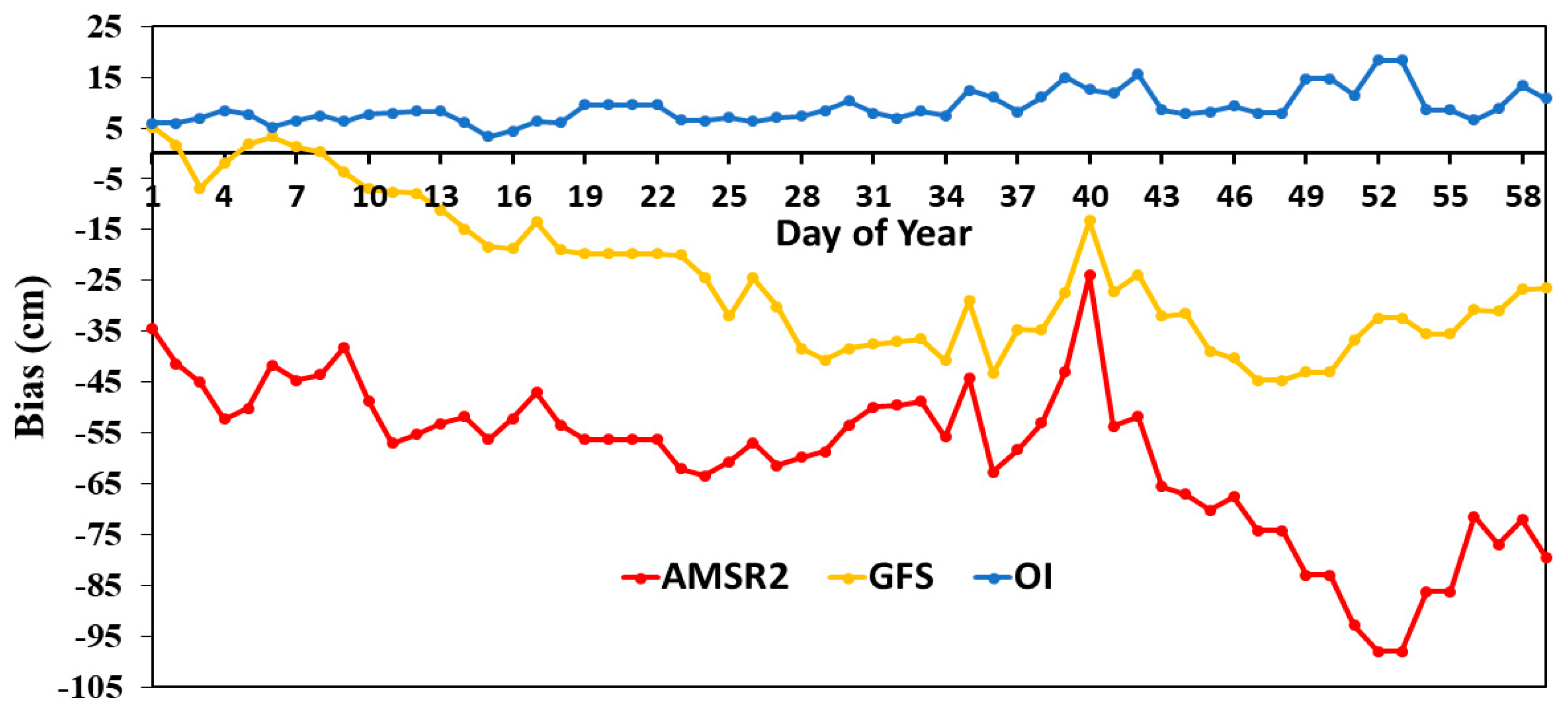
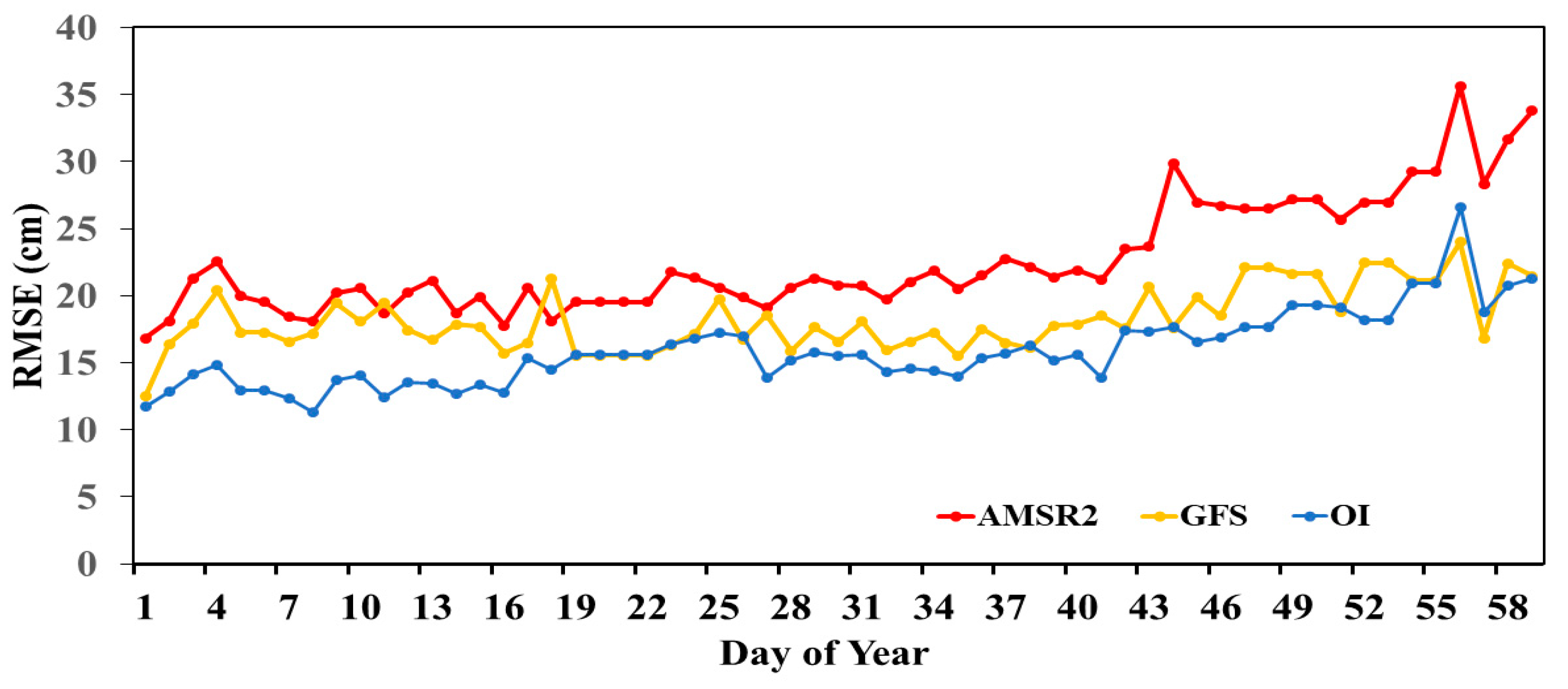
| Snow Depth | Mean/Bias | STD/RMSE | ||
|---|---|---|---|---|
| 7 January | 15 February | 7 January | 15 February | |
| Ground Truth | 23.2 | 28.1 | 19.2 | 22.4 |
| AMSR2 | −7.6 | −7.7 | 18.4 | 27.0 |
| OI | 3.6 | 5.1 | 9.3 | 12.7 |
| GFS | −1.4 | −11.0 | 15.4 | 18.7 |
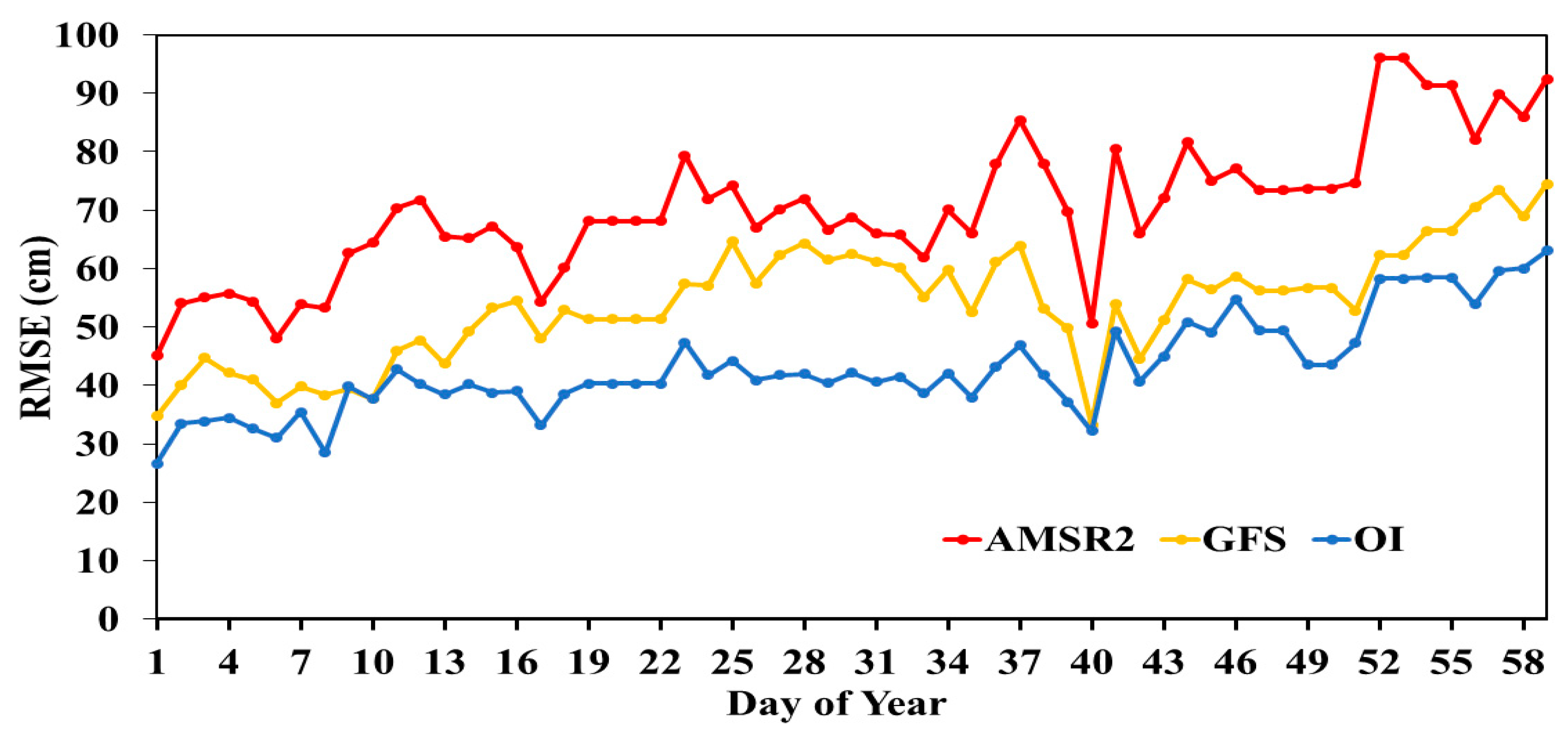
| Snow Depth | Mean/Bias | STD/RMSE | ||
|---|---|---|---|---|
| 7 January | 15 February | 7 January | 15 February | |
| Ground Truth | 62.4 | 88.3 | 51.7 | 75.1 |
| AMSR2 | −44.8 | −68.0 | 52.9 | 78.3 |
| OI | 5.5 | 8.0 | 30.2 | 43.4 |
| GFS | 1.4 | −39.0 | 39.9 | 58.8 |
© 2019 by the authors. Licensee MDPI, Basel, Switzerland. This article is an open access article distributed under the terms and conditions of the Creative Commons Attribution (CC BY) license (http://creativecommons.org/licenses/by/4.0/).
Share and Cite
Kongoli, C.; Key, J.; Smith, T.M. Mapping of Snow Depth by Blending Satellite and In-Situ Data Using Two-Dimensional Optimal Interpolation—Application to AMSR2. Remote Sens. 2019, 11, 3049. https://doi.org/10.3390/rs11243049
Kongoli C, Key J, Smith TM. Mapping of Snow Depth by Blending Satellite and In-Situ Data Using Two-Dimensional Optimal Interpolation—Application to AMSR2. Remote Sensing. 2019; 11(24):3049. https://doi.org/10.3390/rs11243049
Chicago/Turabian StyleKongoli, Cezar, Jeffrey Key, and Thomas M. Smith. 2019. "Mapping of Snow Depth by Blending Satellite and In-Situ Data Using Two-Dimensional Optimal Interpolation—Application to AMSR2" Remote Sensing 11, no. 24: 3049. https://doi.org/10.3390/rs11243049