Satellite Altimetry and Tide Gauge Observed Teleconnections between Long-Term Sea Level Variability in the U.S. East Coast and the North Atlantic Ocean

Abstract

Rising sea levels amplify the threat and magnitude of storm surges in coastal areas. The U.S. east coast region north of Cape Hatteras has shown a significant sea level rise acceleration and is believed to be a “hot-spot” for accelerating tidal flooding. To better understand the forcing mechanism of long-term regional sea level change, in order to more efficiently implement local sea level rise adaptation and mitigation measures, this work investigated the teleconnections between low-frequency sea level variability in the coastal region north of Cape Hatteras and the subpolar/tropical North Atlantic Ocean by using tide gauge measurements, satellite altimetry data and a sea level reconstruction dataset. The correlation analysis demonstrates that the tide-gauge measured sea level variability in the area north of Cape Hatteras is highly and positively correlated with that observed by satellite altimetry in the subpolar and tropical North Atlantic between 1993 and 2002. Over the following decade (2003–2012), the phase of the teleconnection in the subpolar region was reversed and the spatio-temporal correlation in the tropical North Atlantic was enhanced. Furthermore, the positive correlation in the region north of Cape Hatteras’s near shore area is strengthened, while the negative correlation in the Gulf Stream front region is weakened. The North Atlantic Oscillation and Atlantic Multidecadal Oscillation, which affect variations of the Atlantic Meridional Overturning Circulation and Gulf Stream, were shown to have significant impacts on the decadal changes of the teleconnections. Coherent with satellite altimetry data, the reconstructed sea level dataset in the 20th century exhibits similar spatial correlation patterns with the Atlantic Meridional Overturning Circulation, North Atlantic Oscillation and Atlantic Multidecadal Oscillation indices.

1. Introduction

Recently, a significant sea level rise acceleration has been detected along the U.S. east coast north of Cape Hatteras (NCH) using tide gauge data [1,2,3]. The region is also believed to be a “hot-spot” for accelerating tidal flooding [4]. Some studies have revealed that the climate-related changes in the Atlantic Meridional Overturning Circulation (AMOC) and Gulf Stream, as well as the subsistence of the coastal zones are potential drivers behind this [3,5].

Rising sea levels amplify the threat and magnitude of the storm surge-induced urban flooding in coastal areas. Therefore, it is important to combine tide gauge measurements, satellite altimetry and sea level data on longer time series (e.g., the sea level reconstruction) together to better understand the forcing mechanism of the regional sea level variability and help to implement the sea level rise adaptation and mitigation strategy. Yearly averaged tide gauge data have been found to be highly and positively correlated with satellite altimetry data in NCH near shore regions [6]. But are there teleconnections between low-frequency sea level variability in the U.S. east coast and deep-water regions of the North Atlantic (e.g., [7])? If so, how do they link to each other? Do the correlations exist on long time scales? To answer these questions, we investigated the relationships of tide-gauge measured long-term sea level variability to satellite altimetry observations and sea level reconstruction data (1900–2012, [8]) in the North Atlantic.

The paper is organized as follows. The data and methods used in this work are described in Section 2. Section 3 presents the variations of correlations between long-term sea level variability along the U.S. east coast observed by tide gauges and that in the North Atlantic observed by satellite altimeters. Analysis of the factors contributing to the variations are given in Section 4. The results from the sea level reconstruction are shown in Section 5. The summary is presented in Section 6.

2. Data and Methodology

2.1. Satellite Altimetry Data

In this study, we used daily absolute dynamic topography (ADT) data from the SSALTO/Duacs gridded delayed-time products, which were merged from all available satellite altimetry data with spatial resolution of 0.25° × 0.25°. The ADT, known as the sea surface height with respect to the geoid, is a sum of sea level anomaly (SLA) and mean dynamic topography. The daily ADT maps are monthly averaged for further analysis.

2.2. Tide Gauge Data

The monthly sea level data recorded by 32 tide gauge stations (Figure 1) along the U.S. east coast were downloaded from the Permanent Service for Mean Sea Level. The data completeness over the time span of 1993–2012 exceeds 90% at all the tide gauges. The classical inverted barometer correction was applied at each tide gauge station using NCEP (National Centers for Environmental Prediction)/NCAR (National Center for Atmospheric Research) reanalyzed (2.5° × 2.5° grids) monthly sea level pressure data. Considering the high coherent regional sea level variability along the U.S. east coast and to fill the data gaps in the tide gauge measurements, the tide gauges are divided into two groups, i.e., 26 sites in NCH (blue dots in Figure 1) and 6 (black dots in Figure 1) in the region south of Cape Hatteras (SCH) [9]. We averaged the detrended tide gauge data in the two defined regions and the mean value in each composite sea level time series were removed.

To compare with altimetry data and the sea level reconstruction dataset, four representative regions in the North Atlantic Ocean were selected and shown in Figure 1. Significant positive and negative correlations between tide gauge and altimetry data have been found in the NCH near shore area (Region 1) and Gulf Stream front region (Region 2) [6], respectively. Regions 3 and 4 denote the subpolar (e.g., the Labrador Sea) and subtropical regions, respectively.

2.3. Sea Level Reconstruction Data

The reconstructed global sea level by combining sea surface temperature (SST) with tide gauge and altimetry data could represent the contribution of climate variability to sea level change. The data are available over the time period from 1900 to 2012 (see Reference [10] for more details about the dataset). Particularly, the reconstructed sea level variability is highly correlated with the Atlantic Multidecadal Oscillation (AMO) in the North Atlantic Ocean.

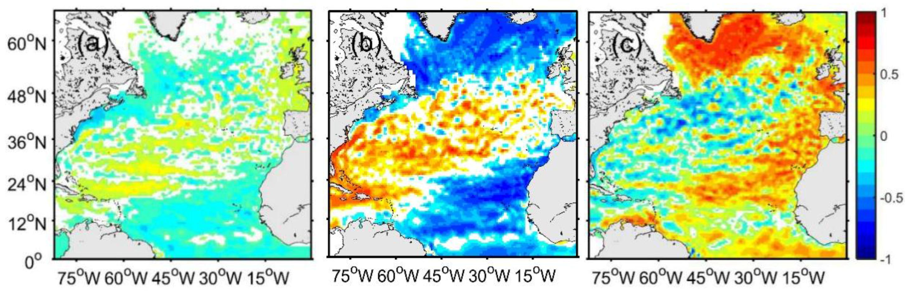
3. Spatio-Temporal Correlations between Sea Level Variability in the U.S. East Coast and the North Atlantic Ocean

In order to show the teleconnections of long-term sea level variability in the U.S. east coast with that in the North Atlantic Ocean, the spatio-temporal correlation coefficients between tide gauge records in SCH (Figure 2a–c)/NCH (Figure 2d–f) and altimeter data at each grid are shown in Figure 2. All the time series were low-pass filtered with a filter half amplitude period of 1 year. To exhibit the changes of the teleconnection patterns on a decadal time scale, the calculations were made over 1993–2012 (Figure 2a,d), 1993–2002 (Figure 2b,e) and 2003–2012 (Figure 2c,f), respectively. Only the correlations significant at 95% confidence level are shown in Figure 2.

In Figure 2a, the SCH averaged sea level variability observed by tide gauges are highly correlated with the altimeter observations in the U.S. near shore areas. Higher correlations are found over these areas in 2003–2012 (Figure 2c) than a decade ago (Figure 2b, 1993–2002). In addition, there is an obvious negative correlation in the sub-polar gyre (e.g., the Labrador Sea and Irminger Sea) in 2003–2012 (Figure 2c), which is not observed in the first decade. This might be due to the possible change in the forcing factors of the regional sea level variability.

Compared with the region SCH, the patterns of the spatio-temporal correlations between altimetry data and tide gauge measurements in NCH (Figure 2d–f) are distinct, indicating the forcing mechanisms are possibly different in these two regions. High correlations are shown from the coasts to the outer shelf and sub-tropical regions (10° N–20° N) in Figure 2d. This has not been investigated in previous works [6]. Compared with the first decade of 1993–2002 (Figure 2e), there is a correlation reversal in the northern North Atlantic and coastal regions of Greenland in 2003–2012 (Figure 2f) and an enhanced correlation in NCH near shore and sub-tropical regions. The change of the high correlations implies a shift from subpolar-related to tropical-related regional sea level variability along the NCH coast in the past two decades. In the following sections, considering that the change of correlation in NCH is more significant than that in SCH and it is a “hot-spot” for accelerating flooding, we focus on the sea level variability in this area.

As shown in Figure 2e, over 1993–2002, the tide gauge data in NCH are negatively correlated with altimeter data near 36° N and 73° W, the southeast of the Gulf Stream’s mean position. This was also pointed out in Reference [6]. However, the correlations disappear in the following decade and a wider spatial coverage of higher correlations exhibits on the NCH shelves, which may be related to the eastward shift of the Gulf Stream path [5].

4. Potential Drivers of the Teleconnection

4.1. Atlantic Meridional Overturning Circulation (AMOC)

In this work, we use a monthly AMOC proxy [11] to investigate the relationship of AMOC to satellite altimetry observations. Figure 3a–c show the spatial pattern of correlations between the AMOC proxy and altimeter data over the time span of 1993–2012, 1993–2002 and 2003–2012, respectively. The white regions denote the correlations that are not significant at the 95% confidence level. In Figure 3a, significant positive correlations appear in the mid-Atlantic Ocean and along the path of the Gulf Stream, while negative correlations are observed in the tropical Atlantic and NCH near shore regions. The comparison of Figure 3c with Figure 3b demonstrates a strengthening of the negative correlations in the U.S. northeast coast, Labrador Sea and tropical North Atlantic in 2003–2012, while the Gulf Stream front (Region 2 in Figure 1) exhibits a weakening of the positive correlation. In the northeastern Atlantic, the correlations reversed in the last two decades.

Compared with Figure 2, one can see the changes of the spatio-temporal correlation patterns agree fairly well with that between the composite tide gauge data in NCH and altimetry data. This indicates the variation in AMOC in recent years is more closely related to sea level variation in the Gulf Stream. Consistent with the other studies (e.g., [12]), the recent weakening of AMOC will increase coastal sea levels but decrease offshore sea levels and lead to higher correlations between tide gauge observed sea level variability in the U.S east coast and altimetry data in the North Atlantic.

4.2. North Atlantic Oscillation (NAO)

The sea level variability in the North Atlantic is highly correlated with NAO [7]. Long term variations of AMOC and Gulf Stream are linked to the NAO index through Ekman transport [13]. Furthermore, the decline of the AMOC proxy in 2009–2010 is linked to the drop in the NAO winter index [14]. Hereby we tested the variations of spatio-temporal correlations between altimeter data and the NAO winter index in the past two decades.

The correlation coefficients between annually averaged altimetry SLA time series and the NAO winter index is shown in Figure 3d–f. The patterns of the correlations in the northern Atlantic Ocean between 1993 and 2002 (Figure 3e) are consistent with that found by [7]. Moreover, negative correlations are found in the NCH near shore region and tropical North Atlantic. However, a significant decrease and an increase in negative correlations are shown in the northern and tropical North Atlantic, respectively, in the following decade (Figure 3f). This is highly consistent with the variations of the correlations between tide gauge and altimeter data over the years (Figure 2e–f).

The similarity between the general patterns of the SLA–AMOC correlation (Figure 3a) and the SLA–NAO correlation (Figure 3d) confirms the close relation between AMOC and NAO as indicated in numerous studies mentioned before. That is also in line with the findings that the sea level variations in the North Atlantic closely represent the AMOC variability driven by the NAO forcing at interannual to decadal time scales [15]. However, some differences in the above correlation patterns in the subpolar region, especially in recent years near the Greenland Sea (Figure 3c), may reveal the influence of some other factors, such as the increase in Greenland ice sheet melt (see Section 2).

4.3. Atlantic Multidecadal Oscillation (AMO)

Figure 3g–i show the variations of spatio-temporal correlations between the SLA and AMO index in the past two decades. An enhancement of the positive correlation is found in the tropical North Atlantic and Labrador Sea in the last decade.

The AMO and NAO indices are not independent of each other. Figure 4a,b show the correlations between a high NAO/AMO index (i.e., outside ± σ of the index, where σ denotes the standard deviation of the index) and altimeter data over 1993–2012. One can see the variability of high station-based NAO is negatively correlated with long-term sea level variability in the northeast Atlantic (Figure 4a). Significant positive correlations between the high AMO index and altimeter data are observed in the Subpolar Gyre and tropical Atlantic Ocean (Figure 4b). Moreover, the correlation coefficients exceed 0.5 in NCH coastal regions. That implies the AMO has an important impact on the variation of long-term sea level variability in the NCH near shore area, whereas a combination of low NAO and high AMO can contribute to higher coastal water levels in this region in the last decade.

To further explain the mechanism of the teleconnection between sea level variability and the AMO/NAO/AMOC, the empirical orthogonal function (EOF) analysis is performed to altimetry data with the trend and seasonal signal removed. The leading EOF mode (EOF1) accounts for 5.4% of the total sea level variance (Figure 5a). The subpolar regions exhibit strong sea level variability accompanied with opposite sea level variability in the Gulf Stream and western subtropical Atlantic. Coherent variability along the NCH and subpolar/subtropical Atlantic regions confirms the teleconnection between sea levels in coastal areas and remote regions in Figure 2d–f.

Figure 5b–d compare the principle component time series (PCTS1) of EOF1 with the negative station-based NAO index, AMO index and negative AMOC proxy, respectively. In Figure 5b, the low-passed NAO (13-month running mean) leads PCTS1 by 6 months. In Figure 5c,d, 13-month and 25-month running means were applied to PCTS1 and AMO/AMOC, respectively, to exhibit the low-frequency sea level variability. Coherent variations are shown between the PCTS1 and the indices with correlations of 0.49, 0.49 and 0.55, respectively. Particularly, the extremely low NAO, high AMO and low AMOC are linked to the strong sea level variation in 2010–2011. Combining Figure 5a with Figure 5b–d explains the decadal variation of the correlations presented in Figure 3, which is associated with the variations of the climate indices.

5. Long-Term Sea Level Variability from Sea Level Reconstruction

In the above sections, we investigated the variations of correlations between tide gauge measurements, altimetry data and climate indices over the period 1993–2012. Does the correlation and teleconnection exist on a longer time scale? Here we try to answer the question based on the reconstructed sea level data over the 20th century (1901–2012).

Before further analysis of the low-frequency sea level variability in the North Atlantic Ocean, we first evaluated the reconstructed sea level data against satellite altimetry data in the four representative regions in Figure 1. The time series of sea level anomaly from the reconstruction dataset and altimeters are shown in Figure 6a–d with trends and seasonal signals removed. All regions exhibit high correlations larger than 0.7. In Figure 6a, the sea level peak in 1998 in Region 1 is captured by the sea level reconstruction dataset. Strong sea level variability in the Gulf Stream is well reproduced (Figure 6b). In the subpolar (Figure 6c) and subtropical (Figure 6d) regions, the correlations exceed 0.8.

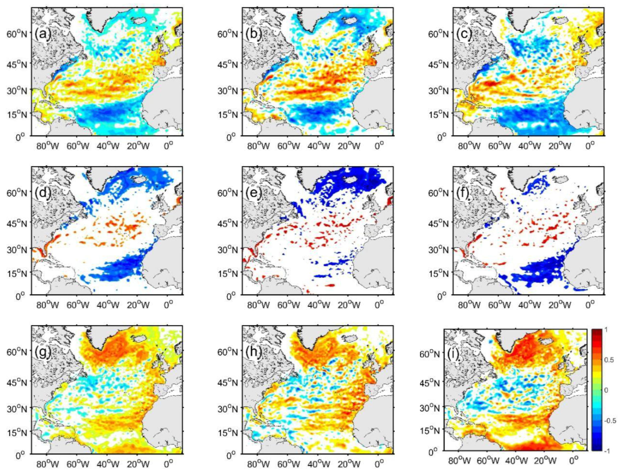
Similar to Figure 3, Figure 7a–c show the correlation coefficient between the filtered sea level reconstruction data and AMOC/NAO winter/AMO indices over 1901–2012 (1935–2012 for AMOC). Compared with the satellite altimetry era (Figure 3a), coherent spatial patterns are observed in the 20th century (Figure 7a) but with a weaker correlation. Comparing Figure 7b with Figure 3d, the reconstructed sea level shows stronger correlation in NCH near shore and subpolar regions. As for the AMO, very similar spatial patterns are presented in altimetry data and the sea level reconstruction dataset (Figure 3g and Figure 7c).

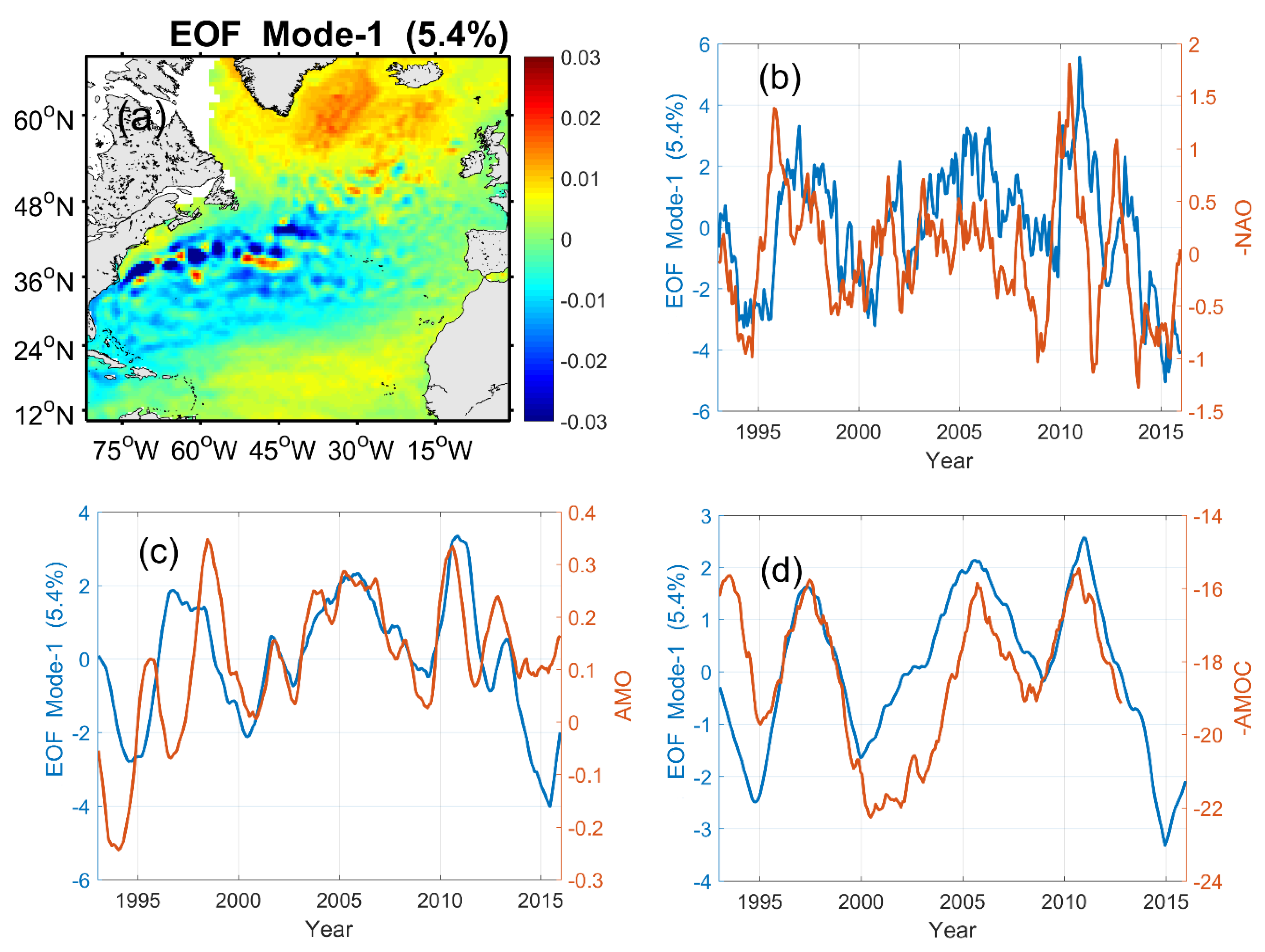
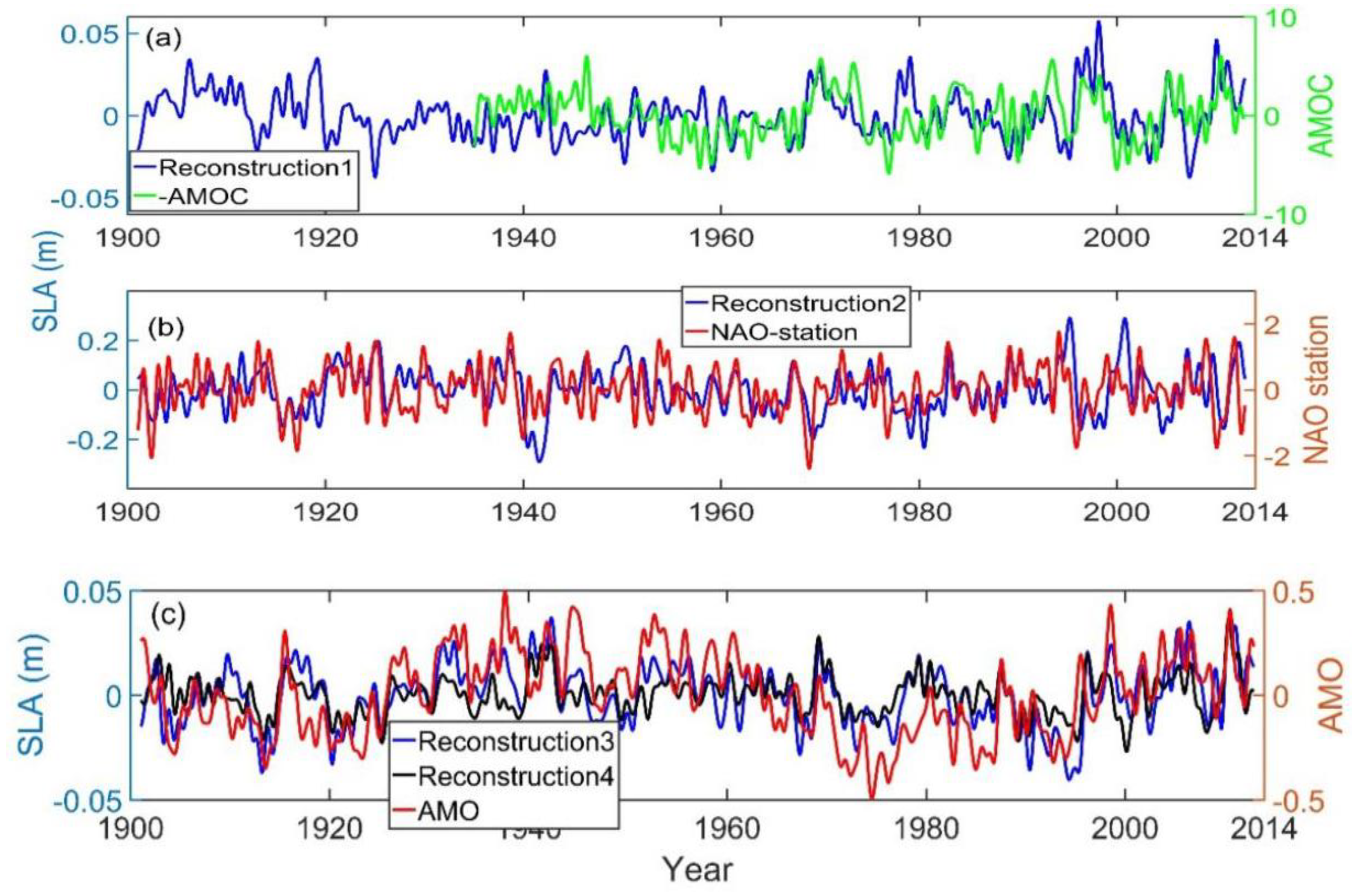
Figure 8 shows the time evolution of the reconstructed sea level anomaly in the past 112 years and AMOC/NAO/AMO indices in the four selected regions. In Figure 8a, a higher correlation could be obtained if the calculation started from 1960. The correlations between the sea level anomalies in the four regions are listed in

Table 1. The correlation coefficient between the sea level reconstructions in the four regions in Figure 1 over 1901–2012. Regions 1–4 denote the NCH near shore area, Gulf Stream front region, subpolar and subtropical North Atlantic, respectively.

	Region 1	Region 2	Region 3
Region 2	−0.45
Region 3	0.38	−0.53
Region 4	0.51	−0.73	0.71

. Negative correlations are found between sea level in the Gulf Stream front and the other three regions, with a correlation coefficient (CC) of −0.45, −0.53 and −0.73, respectively. Sea level variability in the coastal regions are tele-connected with that in the subpolar and subtropical regions with a CC of 0.38 and 0.51. Similar to the altimetry era, the sea level in the subpolar and subtropical regions are highly correlated with each other with an absolute value of CC over 0.7. Combining Figure 8a with Figure 5, it is obvious that the remarkable high sea level variations in NCH coastal regions in 1998–1999 and 2010–2011 are related to AMOC variations and low NAO/high AMO indices.

Table 2. The correlation coefficient between the regional sea level reconstruction and NAO/AMO/AMOC indices over 1901–2012 (1935–2012 for AMOC). Regions 1–4 denote the NCH near shore area, Gulf Stream front region, subpolar and subtropical North Atlantic, respectively.

	NAO	AMO	AMOC
Region 1	−0.30	0.01	−0.37
Region 2	0.38	−0.07	0.21
Region 3	−0.37	0.59	−0.15
Region 4	−0.51	0.38	−0.22

summarizes the correlations between regional sea level reconstructions and the three climate indices. NAO is correlated with the reconstructed sea level in the four regions, but AMO is only correlated with that in the subpolar and subtropical regions. Compared with the other regions, a higher correlation between AMOC and sea level is shown in the NCH near shore area.

6. Summary

In this study, we found a high teleconnection between sea level variability in NCH observed by tide gauges and that captured by satellite altimetry in the subpolar and tropical North Atlantic. The correlation varies on a decadal time scale. In the Labrador Sea, the positive correlations during 1993 to 2002 reverses to negative in the following decade (2003–2012). Compared with the subpolar North Atlantic, satellite data in the tropical region exhibit a stronger connection with tide gauge data in NCH in 2003–2012, which implies a shift of local sea level variability from subpolar-related to tropical-related in the past two decades. Moreover, the negative correlations between tide gauge measurements and altimeter data near 36° N and 73° W disappear in 2003–2012, which could be related to the shift in the Gulf Stream path and has not been reported in previous studies.

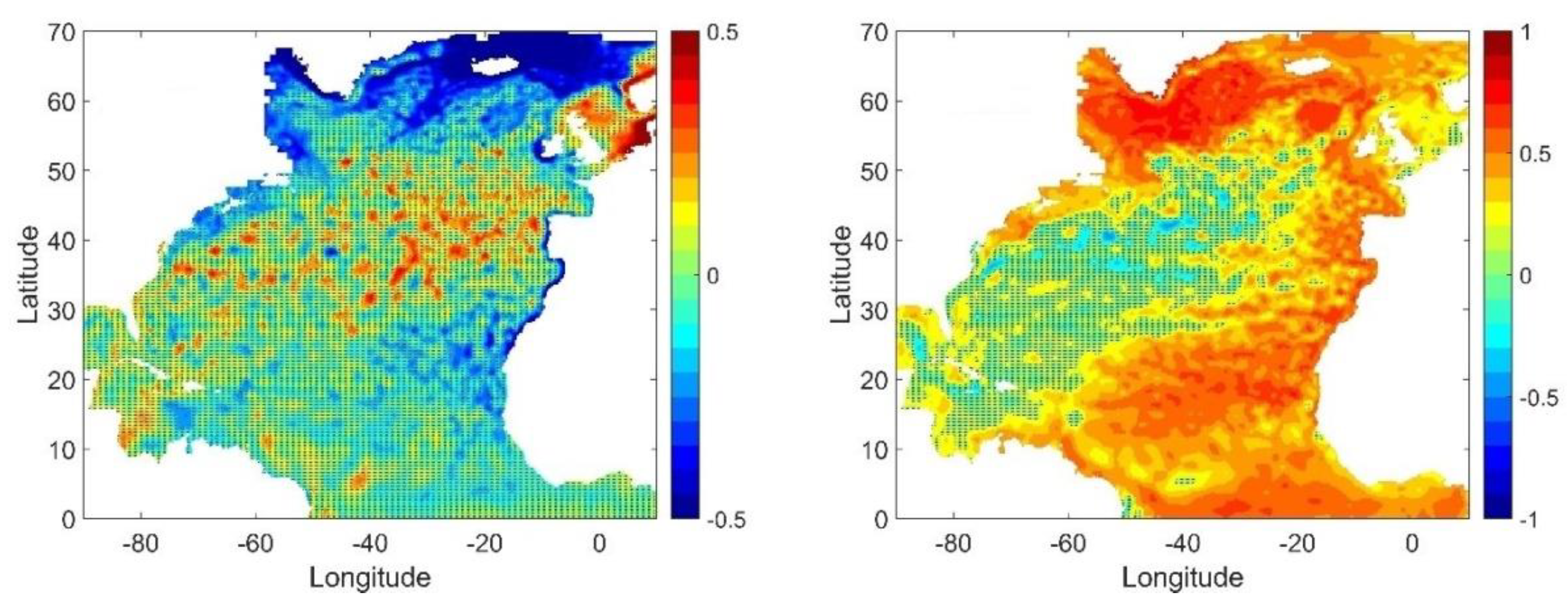
At basin scales, surface heat flux changes contribute a lot to the low-frequency sea level variations [16]. Hence, we further investigated the variability of ocean heat content (OHC) to explain the remote connections between tide gauge and satellite altimeter data in the last 20 years. Figure 9a,b show the distribution of the standard deviation of the detrended OHC over 1993–2002 and 2003–2012, respectively. The AMOC transports the heat from the South Atlantic and tropical North Atlantic to high latitudes. In Figure 9, note the decrease in OHC variability along the Gulf Stream main path, which is possibly related to the slowdown of the AMOC accompanied with less transportation of warm water to the subpolar Atlantic Ocean.

The climatic warming and the melting of the Greenland ice sheet have a great impact on the deep (dense) water formation in the northern North Atlantic and Labrador Sea. The reversed correlations in the Labrador Sea in the last two decades (Figure 2e,f) are consistent with the cooling regions caused by the slowdown of AMOC due to the freshwater anomaly added to the northern North Atlantic [17]. Therefore, the decrease in deep-water formation in the Labrador Sea and the associated reduction of AMOC may partly lead to the correlation variations. In the tropical regions, the areas with positive correlations agree well with the warm westward limb of the AMOC at 10°–20° N. The weakening of AMOC decreases the westward transportation of the warm water. That explains the variability of the sea level here, particularly in 1998, 2005 and 2010 (see Figure 5d).

The variations of the correlations between tide gauge observations in NCH and altimeter data are accompanied with lower or higher negative correlations between NAO winter and annual sea level data in the subpolar and tropical Atlantic Ocean (Figure 3d–f), suggesting that the NAO may be an important factor remotely influencing the local sea level variability.

Another factor linked to the teleconnection of NHC–North Atlantic sea level variability is AMO (Figure 3g–i). A positive AMO phase can increase sea level by thermal expansion, and the associated enhanced AMOC tends to weaken the sea level rise rate in the northeast coastal areas of the U.S. and Subpolar Gyre regions (e.g., [18,19]). The two effects combine to yield the spatial patterns of sea level change associated with the AMO (Figure 4b and Figure 5c). The sea level variability in the NCH near shore area may be linked with that in the subtropical North Atlantic through the observed warming of the tropical Atlantic Ocean (Figure 2h and Figure 4b), and remotely connected with that in the northern North Atlantic through NAO (Figure 4a) and its relationship with AMOC variability.

The climate indices AMOC, AMO and NAO are related to each other. Multidecadal variation of the NAO can induce multidecadal variation of the AMOC and poleward ocean heat transport in the Atlantic (e.g., AMO). The NAO variation could change the AMOC. The sea level reconstruction (1900–2012) demonstrates remarkable decadal sea level variability in the North Atlantic Ocean. Coherent with altimetry data, the reconstructed dataset in the 20th century exhibits similar spatial correlation patterns with the AMOC, NAO and AMO indices (Figure 7 and Table 2). It confirms the teleconnection between sea level variability in NCH and the subpolar/subtropical North Atlantic, which may be attributed to variations in AMOC and NAO/AMO.

References

1. Boon, J.D. Evidence of sea level acceleration at us and Canadian tide stations, Atlantic coast, north America. J. Coast. Res. 2012, 28, 1437–1445. [Google Scholar] [CrossRef]
2. Boon, J.D.; Mitchell, M. Nonlinear change in sea level observed at north American tide stations. J. Coast. Res. 2015, 31, 1295–1305. [Google Scholar] [CrossRef]
3. Sallenger, A.H.; Doran, K.S.; Howd, P.A. Hotspot of accelerated sea-level rise on the atlantic coast of north america. Nat. Clim. Chang. 2012, 2, 884–888. [Google Scholar] [CrossRef]
4. Ezer, T.; Atkinson, L.P. Accelerated flooding along the us east coast: On the impact of sea-level rise, tides, storms, the gulf stream, and the north Atlantic oscillations. Earth Future 2014, 2, 362–382. [Google Scholar] [CrossRef]
5. Ezer, T.; Atkinson, L.P.; Corlett, W.B.; Blanco, J.L. Gulf stream’s induced sea level rise and variability along the us mid-Atlantic coast. J. Geophys. Res. Ocean. 2013, 118, 685–697. [Google Scholar] [CrossRef]
6. Andres, M.; Gawarkiewicz, G.G.; Toole, J.M. Interannual sea level variability in the western north Atlantic: Regional forcing and remote response. Geophys. Res. Lett. 2013, 40, 5915–5919. [Google Scholar] [CrossRef]
7. Volkov, D.L.; van Aken, H.M. Annual and interannual variability of sea level in the northern north Atlantic ocean. J. Geophys. Res. Ocean. 2003, 108. [Google Scholar] [CrossRef]
8. Hamlington, B.; Leben, R.; Strassburg, M.; Kim, K.Y. Cyclostationary empirical orthogonal function sea-level reconstruction. Geosci. Data J. 2014, 1, 13–19. [Google Scholar] [CrossRef]
9. Thompson, P.; Mitchum, G. Coherent sea level variability on the north Atlantic western boundary. J. Geophys. Res. Ocean. 2014, 119, 5676–5689. [Google Scholar] [CrossRef]
10. Hamlington, B.; Leben, R.; Kim, K.Y. Improving sea level reconstructions using non-sea level measurements. J. Geophys. Res. Ocean. 2012, 117. [Google Scholar] [CrossRef]
11. Stepanov, V.N.; Iovino, D.; Masina, S.; Storto, A.; Cipollone, A. Observed and simulated variability of the Atlantic meridional overturning circulation at 41° N. J. Mar. Syst. 2016, 164, 42–52. [Google Scholar] [CrossRef]
12. Ezer, T. Detecting changes in the transport of the gulf stream and the Atlantic overturning circulation from coastal sea level data: The extreme decline in 2009–2010 and estimated variations for 1935–2012. Glob. Planet. Chang. 2015, 129, 23–36. [Google Scholar] [CrossRef]
13. Zhao, J.; Johns, W. Wind-forced interannual variability of the Atlantic meridional overturning circulation at 26.5° N. J. Geophys. Res. Ocean. 2014, 119, 2403–2419. [Google Scholar] [CrossRef]
14. Srokosz, M.A.; Bryden, H. Observing the Atlantic meridional overturning circulation yields a decade of inevitable surprises. Science 2015, 348, 1255575. [Google Scholar] [CrossRef] [PubMed]
15. Li, F.; Jo, Y.-H.; Yan, X.-H.; Liu, W.T. Climate signals in the mid to high latitude north Atlantic from altimeter observations. J. Clim. 2015, 29, 4905–4925. [Google Scholar] [CrossRef]
16. Wang, Z.; Lu, Y.; Dupont, F.; Loder, J.W.; Hannah, C.; Wright, D.G. Variability of sea surface height and circulation in the north Atlantic: Forcing mechanisms and linkages. Prog. Oceanogr. 2015, 132, 273–286. [Google Scholar] [CrossRef]
17. Yin, J.; Goddard, P.B. Oceanic control of sea level rise patterns along the east coast of the United States. Geophys. Res. Lett. 2013, 40, 5514–5520. [Google Scholar] [CrossRef]
18. Hu, A.; Meehl, G.A.; Han, W.; Yin, J. Transient response of the MOC and climate to potential melting of the Greenland ice sheet in the 21st century. Geophys. Res. Lett. 2009, 36. [Google Scholar] [CrossRef]
19. Liu, Z. Dynamics of interdecadal climate variability: A historical perspective. J. Clim. 2012, 25, 1963–1995. [Google Scholar] [CrossRef]
Figure 1. Locations of the tide gauge stations in each group: North (blue dots) and south of Cape Hatteras (black dots). The location of Cape Hatteras (CH) is marked as the red diamond. A water depth of 200 m isobath is overlaid (dashed curve). The red boxes 1–4 denote the four representative regions: the NCH near shore area (1), Gulf Stream front region (2), subpolar (3) and subtropical (4) North Atlantic Ocean.
Remotesensing 11 02816 g001
Figure 2. Geographical distribution of the correlation coefficient between tide gauge measurements south of Cape Hatteras (ac), north of Cape Hatteras (df) and satellite altimeter data over 1993–2012 (left panels), 1993–2002 (middle panels) and 2003–2012 (right panels). The white regions denote correlations that are not significant at the 95% confidence level.
Remotesensing 11 02816 g002
Figure 3. Geographical distribution of the correlation coefficient between the reconstructed monthly AMOC proxy and altimeter observed sea level anomaly (SLA) over the time span of 1993–2012 (a), 1993–2002 (b) and 2003–2012 (c). (df) are similar to (ac) but for correlations between the North Atlantic Oscillation (NAO) winter index and annually averaged altimeter data. (gi) are similar to (df) but for correlations between monthly Atlantic Multidecadal Oscillation (AMO) index and altimeter data. The white regions denote correlations that are not significant at the 95% confidence level.
Remotesensing 11 02816 g003
Figure 4. Geographical distribution of the correlation coefficient between high NAO (left)/AMO (right) index (outside ± σ of the NAO/AMO index) and altimetry sea level time series during 1993 to 2012.
Remotesensing 11 02816 g004
Figure 5. The first empirical orthogonal function (EOF) mode of altimeter SLA in the North Atlantic Ocean (a) and comparison of PCTS1 with NAO (b), AMO (c) and AMOC (d) indices.
Remotesensing 11 02816 g005
Figure 6. Time series of regional mean sea level anomaly from the reconstruction and satellite altimetry in the four representative regions (in Figure 1): (a) the NCH near shore area, (b) Gulf Stream front region, (c) subpolar and (d) subtropical North Atlantic Ocean. The trends and seasonal signals in the time series were removed.
Remotesensing 11 02816 g006
Figure 7. Geographical distribution of the correlation coefficient between the annual averaged reconstructed SLA and monthly AMOC proxy over 1935–2012 (a), NAO winter (b) and AMO indices (c) over the time span of 1901–2012. The white zones denote correlations that are not significant at the 95% confidence level.
Remotesensing 11 02816 g007
Figure 8. Regional mean reconstructed SLA in (a) Region 1: the NCH near shore area; (b) Region 2: Gulf Stream front region; and (c) Regions 3 and 4: subpolar and subtropical North Atlantic Ocean.
Remotesensing 11 02816 g008
Figure 9. Geographical distribution of the standard deviation of the detrended seasonal ocean heat content (10 × 1018 J, 0–700 m) over the time span of 1993–2002 (a) and 2003–2012 (b).
Remotesensing 11 02816 g009