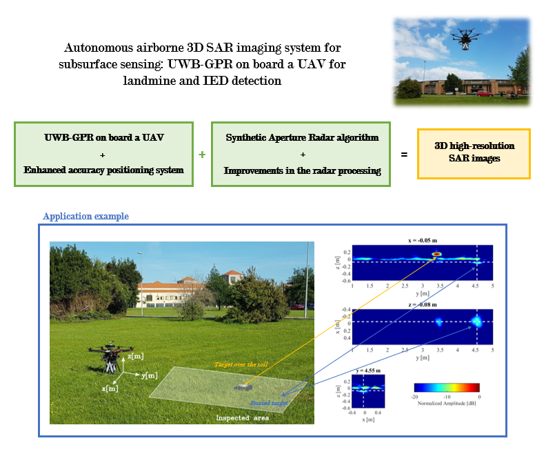
Autonomous Airborne 3D SAR Imaging System for Subsurface Sensing: UWB-GPR on Board a UAV for Landmine and IED Detection

Abstract

This work presents an enhanced autonomous airborne Synthetic Aperture Radar (SAR) imaging system able to provide full 3D radar images from the subsurface. The proposed prototype and methodology allow the safe detection of both metallic and non-metallic buried targets even in difficult-to-access scenarios without interacting with the ground. Thus, they are particularly suitable for detecting dangerous targets, such as landmines and Improvised Explosive Devices (IEDs). The prototype is mainly composed by an Ultra-Wide-Band (UWB) radar module working from Ultra-High-Frequency (UHF) band and a high accuracy dual-band Real Time Kinematic (RTK) positioning system mounted on board an Unmanned Aerial Vehicle (UAV). The UAV autonomously flies over the region of interest, gathering radar measurements. These measurements are accurately geo-referred so as to enable their coherent combination to obtain a well-focused SAR image. Improvements in the processing chain are also presented in order to deal with some issues associated to UAV-based measurements (such as non-uniform acquisition grids) as well as to enhance the resolution and the signal to clutter ratio of the image. Both the prototype and the methodology were validated with measurements, showing their capability to provide high-resolution 3D SAR images.

1. Introduction

In the last years, there has been a massive development of new applications using Unmanned Aerial Vehicles (UAVs) [1,2,3,4]. A considerable amount of these applications is based on integrating electromagnetic sensors on board the UAVs (e.g., power detectors for antenna measurement [5], or radars for earth observation [6] and subsurface sensing [7]). Safety, measurement speed and the ability to fly over difficult-to-access areas are some of the advantages that have contributed to widely increase the usage of UAVs for security and defense applications, such as landmine and Improvised Explosive Device (IED) detection.

Several Non-Destructive Testing (NDT) techniques have been employed for subsurface sensing applications, since they allow extracting information of the subsurface and detecting possible buried targets without interacting with them. Focusing on the field of landmine and IED detection, the most common NDT techniques are, according to their physical principle [8]: electromagnetic induction, Nuclear Quadrupole Resonance (NQR), thermal imaging and Ground Penetrating Radar (GPR). GPR has been found to be a useful strategy for this application since it is able to provide high resolution images from the subsurface and, as a result, it makes possible the detection of both metallic and dielectric buried targets [9,10]. However, GPR capabilities are considerably affected by the soil heterogeneity, the roughness of the air–soil interface and the possible low signal to clutter ratio (especially for non-metallic targets) [11].

There are several criteria to classify GPR systems. The first criterion takes into account whether the GPR antennas are placed directly in contact with the ground (ground-coupled) or above the ground (air-launched). The former architecture usually provides a better signal to clutter ratio, due to a higher penetration into the ground and weaker reflections from the air–soil interface (assuming a well-matching between the antennas and the soil impedance). The main drawback of this configuration is that the antennas are directly over the soil, which prevents the use of ground-coupled systems in applications which require a safety stand-off distance such as the aforementioned landmine and IED detection. The latter architecture avoids the contact with the ground, but suffers from stronger clutter, which makes the target detection more difficult. Another criterion classifies GPR systems according to the orientation of the antennas with respect to the soil surface, distinguishing between Forward (or Side)-Looking GPR (FLGPR, SLGPR) and Down-Looking GPR (DLGPR). In FLGPR [12] and SLGPR [13], the antennas are usually oriented looking ahead, which contributes to minimize the reflection coming from the air–soil interface. Nevertheless, they suffer from lower sensitivity and resolution (compromising the distinction between targets under or above the ground). On the other hand, in DLGPR [14], the antennas are placed looking downwards, providing higher resolution but receiving stronger reflections from the air–soil interface.

As aforementioned, in landmine and IED detection, the scanning system must be placed at a safe stand-off distance to prevent accidental detonations, thus FLGPR architectures have been usually proposed due to the difficulties to keep a safe distance with a DLGPR system. However, in the last years, a new approach based on a UAV-mounted radar has been proposed [7,15], allowing the use of a DLGPR configuration in safe conditions.

Although several UAV-mounted GPR systems have been presented [7,16,17], the system and processing techniques presented in this contribution have several novelties with respect to existing state-of-the-art systems. The most important feature is its ability to provide high resolution well-focused 3D images of the underground from radar measurements gathered during autonomous flights. This requires integrating a high accuracy real-time positioning system on board the UAV because: (i) the UAV needs accurate positioning to follow the predefined flight path; and (ii) the radar measurements are coherently combined using a Synthetic Aperture Radar (SAR) algorithm, which imposes a geo-referring accuracy several times lower than the smallest working wavelength. Furthermore, the positions of the radar measurements are carefully processed to discard data that could cause unfocusing or resolution degradation in the SAR image (for instance, due to oversampling in some areas [18], since it is very difficult to perform a uniformly sampled acquisition with the UAV). Regarding the processing of the radar data, some improvement steps are also proposed to enhance the resolution and the target discrimination. In addition, the lowest working frequency of the selected radar has been notably decreased (down to Ultra-High-Frequency, UHF, band), allowing the detection of targets buried in higher loss soils. Both the prototype and the processing techniques were tested with experimental flights, comparing the resulting 3D SAR images with the ground-truth. A video summarizing the features of the system and a brief application example is provided as Supplementary Materials.

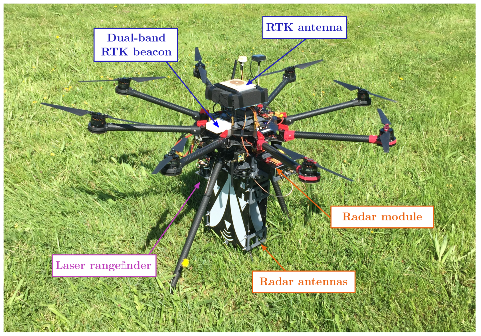
2. System Architecture

The main goal of the proposed system is that the UAV autonomously flies over a region of interest collecting radar measurements, which are geo-referred and sent in real-time to a ground control station, to produce high-resolution 3D SAR images. The UAV-mounted GPR prototype, which is shown in Figure 1, comprises the following subsystems:

• The flight control subsystem is composed of the UAV flight controller and common positioning sensors on board UAVs. These sensors are: an Inertial Measurement Unit (IMU), a barometer, and a Global Navigation Satellite System (GNSS) receiver.
• The enhanced positioning system consists of a laser rangefinder and a dual-band Real Time Kinematic (RTK) system.
• The radar subsystem includes the radar module, and the transmitter and receiver antennas.
• The communication subsystem has a receiver at 433 MHz for the link with the pilot remote controller and a wireless local area network (WLAN) transceiver at $5.8$ GHz to exchange data with the ground station. Both frequencies were selected to minimize possible interferences with the radar subsystem during the experimental campaigns.

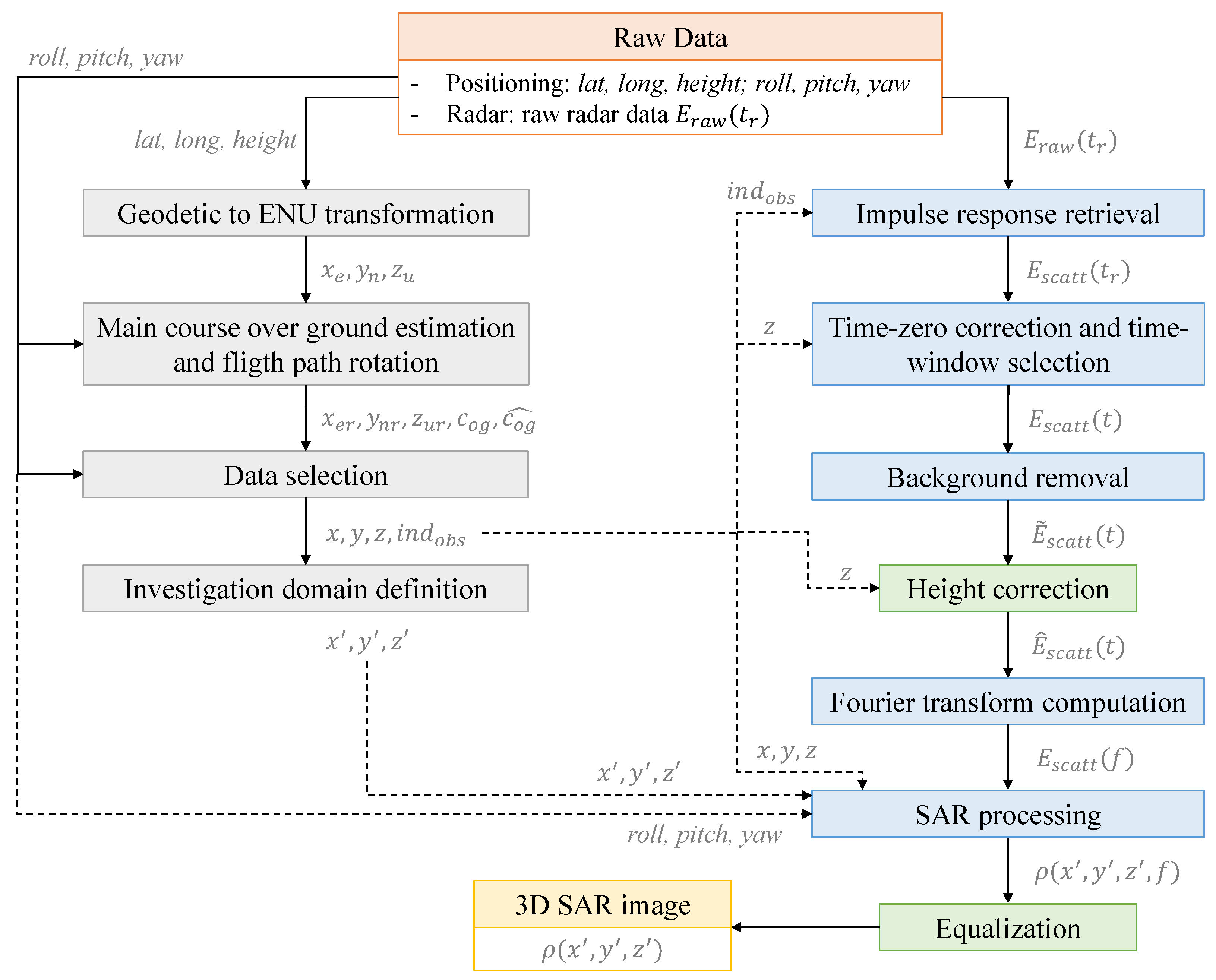
The architecture of the system is similar to the one adopted by the prototype proposed in [7]. The main improved features are: (i) the radar subsystem, which works at considerably lower frequencies; and (ii) the enhanced positioning system, whose accuracy has been greatly increased. As a result, with the prototype presented in this contribution, targets buried in soils with higher losses can be detected and, due to the enhanced positioning accuracy, well-focused 3D SAR images of the underground can be obtained.

Regarding the radar subsystem, an M-sequence Ultra-Wide-Band (UWB) radar covering a frequency range from 100 MHz to 6 GHz was selected [19]. This radar transmits a type of pseudo-random binary signal called Maximum Length Binary Sequence (MLBS) periodically, thus the received backscattered signal must be correlated with the ideal MLBS to obtain the impulse response. Two UWB Vivaldi antennas, working from 600 MHz to 6 GHz, were selected for transmitting and receiving. For the experimental validation shown in this contribution, only the frequency band from $f_{\min }=600$ MHz to $f_{\max }=3$ GHz was selected for processing since the soil losses in the measured scenario produce too much attenuation at higher frequencies. As shown in Figure 1, 3D printed structures were designed and fabricated to properly mount the radar and the antennas on board the UAV.

Concerning the enhanced positioning system, to coherently combine all the measurements gathered with the prototype, they must be accurately geo-referred. To avoid artifacts and obtain a well-focused SAR image, this accuracy should be better than ${\lambda }_{\min }/4=2.5$ cm in the horizontal plane (i.e., in cross-range) and ${\lambda }_{\min }/8=1.25$ cm in the vertical direction (i.e., in range), where ${\lambda }_{\min }=10$ cm is the smaller wavelength. A dual-band multiconstellation RTK system was selected to fulfill this requirement. This system is composed of two RTK beacons [20], one mounted on the UAV and another one working as base station static on the ground. The latter sends real-time correction data to the former to achieve cm-level positioning accuracy. The reason a dual-band RTK was chosen is to obtain better accuracy and availability (that is, percentage of time that corrected coordinates are provided), more robustness (especially when working in challenging environments, e.g., with limited sky view) and faster deployment time (since less time is required to resolve carrier phase ambiguity), compared to single-band RTKs previously used. The selected dual-band RTK was integrated into the UAV to provide these accurate coordinates in real time for both the UAV navigation and the measurements geo-referring. The expected accuracy is $0.5$ cm in the horizontal plane and 1 cm in the vertical direction, which corresponds to ${\lambda }_{\min }/20$ and ${\lambda }_{\min }/10$, respectively. Nevertheless, even better relative positioning accuracies were observed during the measurement campaigns.

3. Methodology

The data acquired with the prototype (composed by the georeferred radar measurements) are processed according to the flowchart shown in Figure 2. The boxes in gray correspond to the processing of the geo-referring data gathered with the positioning subsystem, blue boxes represent the basic GPR-SAR processing, and green ones highlight the steps corresponding to improvements in the GPR-SAR processing. The final result is a 3D high-resolution SAR reflectivity image (yellow box).

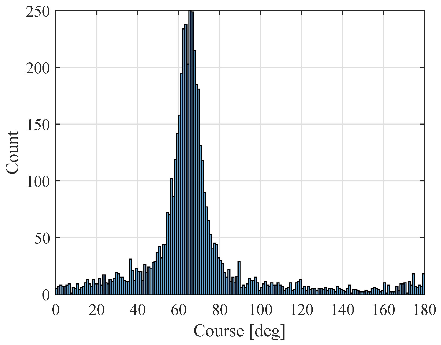
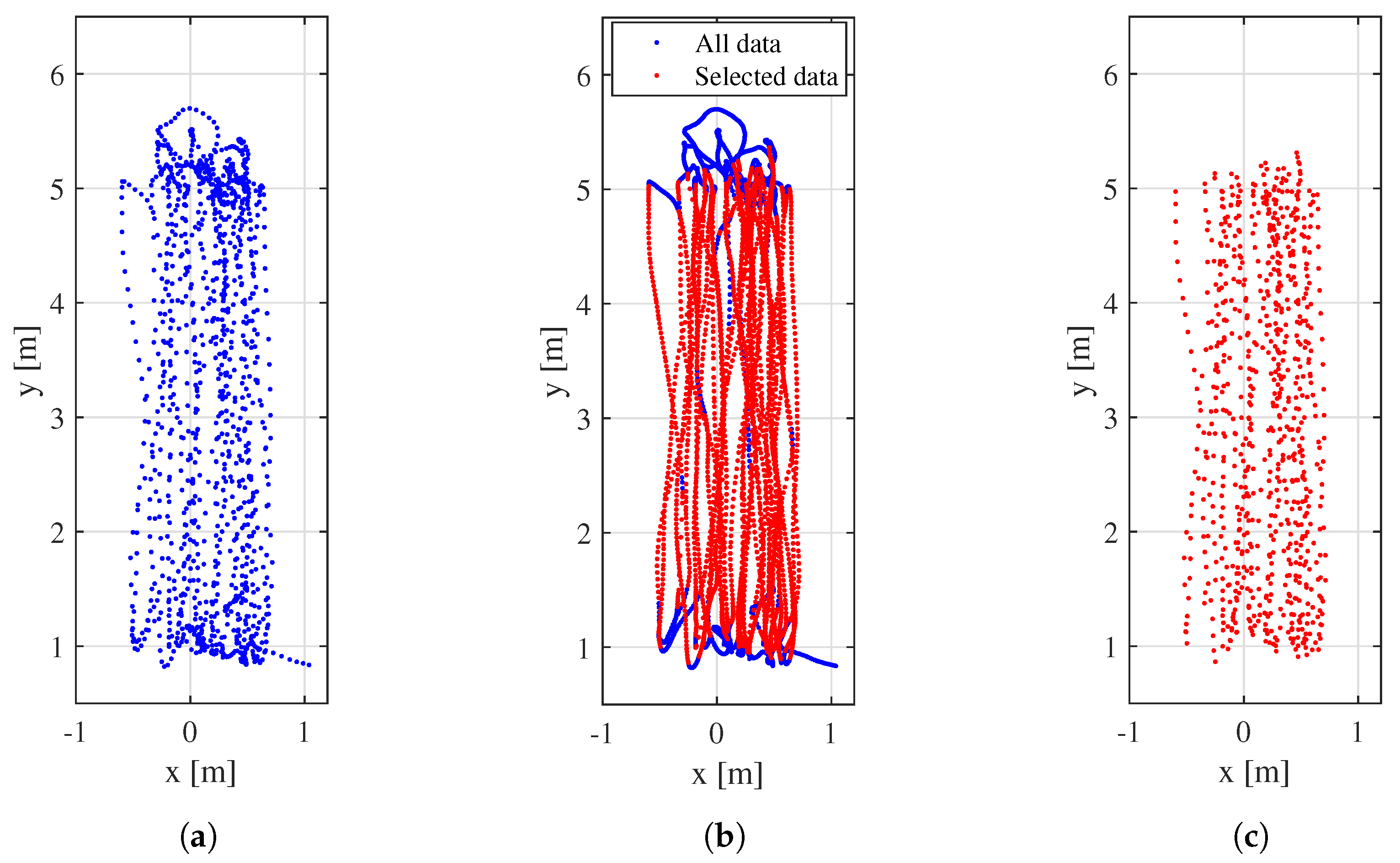
3.1. Positioning Data Processing

The flowchart of the positioning data processing is shown in Figure 2 (left). The positioning data to be processed is composed by: latitude (lat), longitude (lon) and height from the RTK system, and roll, pitch and yaw from the IMU. Due to the high accuracy of the RTK system in both horizontal and vertical directions, the laser rangefinder is not used in the processing. It is used, however, in the UAV navigation to help the UAV to keep an approximately constant distance to the soil surface.

This geo-referring data are processed mainly: (i) to select which measurements will be processed (discarding those that do not provide valuable information); (ii) to compute the position of the radar antennas in a cartesian coordinate system; and (iii) to define the investigation domain (i.e., where the SAR image is obtained) according to the flight path.

As explained above, the UAV autonomously flies over the region of interest. The flight path (i.e., the measurement grid) is a planar rectangular surface at a constant height and heading, where geo-referred radar measurements are continuously collected. However, it must be noticed that the proposed positioning data processing does not require prior knowledge of the predefined measurement grid, thus allowing the processing of measurements gathered in planar grids with both autonomous and manual flights.

The first step consists of transforming the coordinates from the geodetic system (latitude, longitude and height) to a local ENU (East–North–Up) system ($x_e$, $y_n$, $z_u$). This requires selecting a reference point as origin of the ENU system. In particular, the position of the UAV when it is first turned on is used as reference: the latitude and the longitude are given by the RTK, and the height is given by the physical distance from the RTK antenna to the ground (so that at the reference position, $z_u=0$ m).

Then, the main course over the ground or main ground track (denoted as $\widehat{c_{og}}$) is estimated and the flight path is rotated according to this value. After the rotation, the flight path will be almost aligned with the x- and y-axis, which helps to facilitate the visualization of the measurements and the definition of the investigation domain. $\widehat{c_{og}}$ will also be used in the next step (data selection) to discard measurements acquired when the course over the ground is too far from its main value.

The main ground track estimation is obtained from the set of UAV positions as follows: (i) the course over the ground $c_{og}$ (discarding the sense) is computed according to Equation (1), where $v_n$ and $v_e$ are the velocities in the north and east directions and mod denotes the modulo operation; (ii) $c_{og}$ is discretized in bins of $1^{\circ }$-width and the mode is computed to obtain a rough estimation of the main course over the ground $\widetilde{c_{og}}$; and (iii) the estimation is improved by computing the mean of all measurements in the range $\widetilde{c_{og}}\pm {10}^{\circ }$, yielding $\widehat{c_{og}}$. If the flight path is performed autonomously (as in this contribution), this value is almost the same as the desired course defined with the waypoints. It must be noticed that the mean of $c_{og}$ is a worse estimation of the main course over the ground than $\widehat{c_{og}}$, since it is greatly influenced by the course of the UAV when it changes sense or when it is almost still.

$$c_{og}\left[rad\right]=\mathrm{mod}\left(\mathrm{atan}\left(\frac{v_n}{v_e}\right),\pi \right)\approx \mathrm{mod}\left(\mathrm{atan}\left(\frac{\partial y_n}{\partial x_e}\right),\pi \right)$$

(1)

Figure 3 shows the histogram of $c_{og}$ of an autonomous flight defined with waypoints (with a desired course of ${65}^{\circ }$). The mode gives the rough estimation of $\widetilde{c_{og}}={65.5}^{\circ }$. After improving this estimation as explained before, $\widehat{c_{og}}={65.09}^{\circ }$, which is almost the same as the desired course. The original and rotated flight paths are shown in Figure 4. As expected, the rotated path ($x_{er}$, $y_{nr}$, $z_{ur}$) is now aligned with the x- and y-axis.

The next step aims to discard the data that do not provide valuable information (e.g., when there is a sudden change in attitude) or that could degrade the SAR image. Regarding the latter, it must be noticed that the spatial sampling should be as uniform as possible to avoid artifacts in the SAR image. If there is an oversampled region (where much more measurements were taken), the SAR image pixels close to this region will have a high amplitude, thus masking the detection of targets in other parts of the image. In measurements taken with UAVs, it is very difficult to perform a uniform acquisition, since the UAV deviates from the ideal flight path mainly due to wind conditions and positioning systems uncertainties. Furthermore, in the experimental flights, it was observed that, when the UAV changes sense of movement (i.e., when it changes from moving in one direction to moving in the opposite one), the speed usually decreases, thus resulting in oversampling. It must be remarked that the UAV heading is fix to a constant value (making it coincident with the desired main course over the ground).

The data that are kept for further processing must satisfy the following constraints, where $t{h}_{\left(\right)}$ denotes a fix threshold:

• ${\Delta }_{xy}=\sqrt{\Delta x_{er}^2+\Delta y_{nr}^2}>t{h}_{\Delta }$, where $\Delta x_{er}$ and $\Delta y_{er}$ are the differences between adjacent values of $x_{er}$ and $y_{er}$, respectively. This condition ensures that the UAV is actually moving.
• $|roll-\overline{roll}|<t{h}_{roll}$, $|pitch-\overline{pitch}|<t{h}_{pitch}$, and $|yaw-\overline{yaw}|<t{h}_{yaw}$, where $\overline{\left(\right)}$ denotes the mean value. These conditions are used to filter out the positions where there was a noticeable change in attitude.
• $|\mathrm{rem}(c_{og}-\widehat{c_{og}},\pi )|<t{h}_c$, where $\mathrm{rem}$ denotes the remainder operator. Only measurements with the course over ground close to the main one are kept. This means that, if the UAV path deviates noticeably from the main path, these measurements are discarded.
• $|z_{ur}-\overline{z_{ur}}|<t{h}_z$. This condition helps to get rid of considerable changes in height.

The following thresholds were employed: $t{h}_{\Delta }={\lambda }_{\min }/6\approx 0.017$ m (where ${\lambda }_{\min }$ is the smaller wavelength), $t{h}_{att}=\overline{att}+3\mathrm{std}\left(att\right)$ where $\mathrm{std}$ is the standard deviation and $att$ is each of the attitude angles (roll, pitch and yaw), $t{h}_c={20}^{\circ }$ and $t{h}_z=0.25$ m. They were found to provide a good compromise to avoid oversampling and discard unnecessary data, while keeping enough measurements to obtain a well-focused SAR image.

In the flight used for illustrating the positioning data processing, the UAV is mainly moving back and forth between $y=1$ m and $y=5$ m. If only one of each four consecutive UAV positions are plotted (Figure 5a), it can be clearly seen the oversampling when the UAV changes sense of movement (at $y=1$ m and $y=5$ m). Figure 5b shows the full flight path (after the rotation performed in the previous step) and the selected flight path. Most of the discarded data correspond to these oversampled regions (as can be inferred from Figure 5c), whereas the rest of discarded data mainly correspond to sudden changes in movement due to wind.

This data selection step also helps to reduce the number of measurements that are processed, thus helping to decrease the computational time. In the previously shown example, the full flight path contains 4993 measurements points, whereas the selected path has 3118 points. This means that only $62.5\%$ of the measurements will be processed.

As a result of this step, the indexes of the measurements that will be processed $\left(in{d}_{\mathrm{obs}}\right)$ are stored in a vector. Thus, the observation domain coordinates (i.e., the positions where these measurements were taken) are: $\mathit{r}=(x,y,z)$, where $x=x_{er}\left(in{d}_{obs}\right)$, $y=y_{nr}\left(in{d}_{obs}\right)$ and $z=z_{ur}\left(in{d}_{obs}\right)$.

Finally, the investigation domain, ${\mathit{r}}^{\prime }=(x^{\prime },y^{\prime },z^{\prime })$, where the 3D SAR image will be calculated must be defined. The investigation plane ($x^{\prime }$ and $y^{\prime }$ coordinates) is defined according to the observation plane (x and y coordinates) as follows:

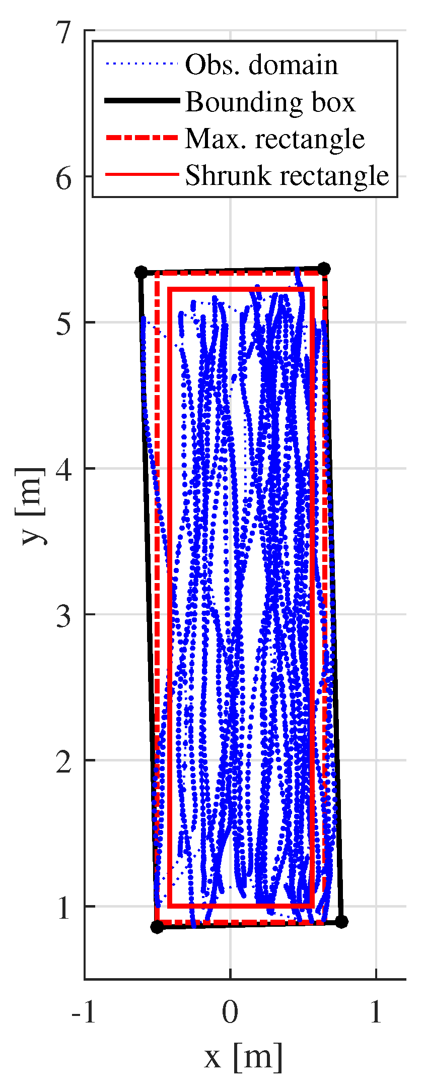
• First, the minimum area bounding rectangle that encloses the observation plane (called bounding box) is retrieved. To find it, the convex hull of the observation plane coordinates (i.e., the smallest convex polygon containing the observation plane) is computed. Then, the bounding box can be easily obtained since it always contains an edge of the convex hull.
• Then, the maximum axis-aligned rectangle inside the bounding box is computed, since it is easy to define and work with an axis-aligned investigation domain and the observation domain is almost aligned (due to the rotation according to the main course over the ground previously performed).
• Finally, the investigation plane is defined by shrinking this rectangle by a scale factor of $s{f}_t$ and $s{f}_{ct}$ in the track and across-track directions (to avoid edge effects in the SAR image) and sampling it every ${\delta }_t$ and ${\delta }_{ct}$, respectively.

An example of the computation of the investigation plane following this procedure is shown in Figure 6, where the bounding box is depicted with a solid black line, the maximum axis-aligned rectangle inside it is drawn with a dash-dot red line and the edges of the investigation plane are shown in solid red. For the results shown in this contribution, the investigation plane is obtained by shrinking the rectangle with the scale factors $s{f}_t=0.95$ and $s{f}_{ct}=0.85$ (which prevents edge effects in the SAR image) and sampling it every ${\delta }_t={\delta }_{ct}={\lambda }_{\min }/4=0.025$ m. Since the soil surface is around $z=0$ m, $z^{\prime }$ is defined between $-0.6$ m and $0.4$ m, and is sampled every ${\delta }_z=0.02$ m. These values can be adjusted by the user as desired (e.g., if coarse sampling of the investigation domain is considered enough for the specific application considered).

It is worth noting that the investigation domain coordinates, ${\mathit{r}}^{\prime }=(x^{\prime },y^{\prime },z^{\prime })$, where the 3D SAR image is calculated, can be transformed back to the geodetic system of coordinates by applying the inverse of the previous operations (i.e., rotating them an angle $-\widehat{c_{og}}$ and then applying the transformation from the local east–north–up system to the geodetic system).

3.2. Radar Data Processing

The flowchart of the radar data processing is shown in Figure 2 (right). As aforementioned, the boxes in blue correspond to the basic processing and the boxes in green are optional steps to improve the resulting SAR image quality.

Since the radar used in this contribution transmits a pseudorandom binary sequence, the first step consists of cross-correlating the raw radar data $E_{raw}\left(t_r\right)$ with the ideal transmitted binary sequence to obtain an approximation of the impulse response function $E_{scatt}\left(t_r\right)$ (where $t_r$ is the time axis). As explained above, it must be noticed that only the selected measurements (given by $in{d}_{obs}$) will be processed.

The next step deals with adjusting to a common time-zero and selecting the time-window of interest. Estimating the time-zero is important in order to remove the effect of the wires and the radar internal delays as well as to obtain a well-focused image. The estimation is performed with a calibration measurement at the beginning of the experimental campaign. The prototype is placed over the ground at a known distance ($d_{rg}$) and this distance is also estimated with the radar ($d_{eg}=c{t}_g/2$, where c is the light speed and $t_g$ is the time instant where the ground is detected). Therefore, the time-zero is given by $t_0=2(d_{eg}-d_{rg})/c$, the corrected time-axis is $t_c=t_r-t_0$ and the measurements at $t_c<0$ will be discarded. Besides, the time window of interest is selected so as to reduce the data size (since measurements at larger range do not provide valuable information). In particular, the used criterion selects the time-window t that corresponds to a range of $\overline{r_0}\pm 1$ m, where $\overline{r_0}$ is the mean distance between the radar antennas and the soil. It must be remarked that the time-zero is estimated only once, and then the same time-zero correction is applied to all measurements (discarding the data at $t_c<0$).

The radar measurements of the flight shown in Section 3.1 after applying this step are depicted in Figure 7, where the range axis is given by $r_{ng}=ct/2$.

To improve the signal to clutter ratio [21], the background should be estimated and removed from the radar measurements. In this contribution, the background is estimated as the average of all measurements and thus, the average is subtracted from each measurement. This helps to reduce the clutter, such as the coupling effects between the antennas.

The resulting improved radar measurements ${\tilde{E}}_{scatt}\left(t\right)$ are shown in Figure 8, where a clear improvement can be noticed comparing this image with the original radar data. This enhancement can be better observed taking a closer look to both original and improved radar measurements (Figure 9). Furthermore, there is a good agreement between the location of the air–soil interface in the radar measurements and the distance between the radar antennas and the soil provided by the positioning system. The small discrepancies are mainly due to the soil being not perfectly flat (besides the scattering effects due to the presence of grass on the ground), and the errors in the positioning system.

After this step, a height correction can be applied to the data to enhance the SAR image quality (mainly focusing and resolution). This correction consists of first shifting the radar measurements by $z-\overline{z}$, so that the resulting data ${\widehat{E}}_{scatt}\left(t\right)$ look as if the measurements were taken at constant height.

The radar measurements after the height shifting are shown in Figure 10 and a closer look is depicted in Figure 11. As expected, the strong reflection at the air–soil interface is now almost at the same range for all measurements. In addition, it can also be concluded that there is a target at around 15 cm over the ground.

After the shifting, a second background subtraction is applied to mitigate the reflection from the air–soil interface and further enhance the signal to clutter ratio.

The next step consists of applying the Fourier transform to obtain $E_{scatt}\left(f\right)$ since the SAR processing will be performed in the frequency domain. Before the SAR processing, the positions of the transmitter and receiver antennas, denoted as ${\mathit{r}}_t=(x_t,y_t,z_t)$ and ${\mathit{r}}_r=(x_r,y_r,z_r)$, must be calculated since the observation domain coordinates are given with respect to the RTK antenna. These positions are computed through translation and rotation operations taking into account the attitude angles, the observation domain coordinates and the distances between the RTK antenna, the radar antennas and the IMU. If height correction has been applied, this must also be taken into account since in this case $z=\overline{z}$.

Then, a SAR algorithm [22] is applied to coherently combine the measurements and obtain a well-focused image. SAR reflectivity at pixel ${\mathit{r}}_p^{\prime }$ is given by Equation (2), where $f_n$ are the selected frequencies of interest; ${\mathit{r}}_t^m$ and ${\mathit{r}}_r^m$ denote the position of the transmitter and receiver antennas, respectively, at the mth measurement point; $k_{0,n}$ is the wavenumber in free-space at the nth frequency; and $R_{p,m}$ is the total path length between the transmitter antenna, the pixel where the SAR reflectivity is computed and the receiver antenna.

$$\rho \left({\mathit{r}}_p^{\prime }\right)=\sum _{n=1}^N\rho ({\mathit{r}}_p^{\prime },n)=\sum _{n=1}^N\sum _{m=1}^M{E}_{scatt}(f^n,{\mathit{r}}_t^m,{\mathit{r}}_r^m)\exp (+j{k}_{0,n}{R}_{p,m})$$

(2)

If free-space propagation is assumed (i.e., the soil composition is not taken into account), then $R_{p,m}=\parallel {\mathit{r}}_t^m-{\mathit{r}}_p^{\prime }\parallel +\parallel {\mathit{r}}_r^m-{\mathit{r}}_p^{\prime }\parallel$. Thus, if an object is buried at $d_{obj}$ depth and the soil permittivity is ${\epsilon }_r$, it will be detected at $\sqrt{{\epsilon }_r}{d}_{obj}$ in the SAR image. To consider the soil composition when calculating the path length for $z_p^{\prime }<0$ m (i.e., under the soil surface), $R_{p,m}$ is computed according to (3), where $n_s=\sqrt{{\epsilon }_r-1}-\sqrt{{\epsilon }_r}$ and the other parameters are shown in Figure 12 [23].

$$R_{p,m}=2d\sqrt{{\epsilon }_r-1}+\frac{d_t(d_t-d{n}_{s}cos\left(2{\varphi }_t\right))}{d_t+d{n}_{s}sin{\left(2{\varphi }_t\right)}^2}+\frac{d_r(d_r-d{n}_{s}cos\left(2{\varphi }_r\right))}{d_r+d{n}_{s}sin{\left(2{\varphi }_r\right)}^2}$$

(3)

To improve the resolution of the SAR image, an equalization of the frequency response can be performed. When working with UWB radars and antennas, the amplitude levels of the SAR image show a great variation across the whole frequency band (mainly due to the fact that the antenna behaviour notably changes with the frequency) [19]. Usually, the data at lower frequencies mask the data at higher frequencies, yielding a SAR image with worse resolution than expected. To overcome this issue, instead of computing the SAR image for all the frequencies directly, the SAR image is computed for each nth frequency and is normalized by the maximum of its absolute value. Then, all nth SAR images are added to obtain the final SAR image, according to Equation (4).

$$\rho \left({\mathit{r}}_p^{\prime }\right)=\sum _{n=1}^N\frac{\rho ({\mathit{r}}_p^{\prime },n)}{max\left\{\right|\rho ({\mathit{r}}_p^{\prime },n)\left|\right\}}$$

(4)

4. Results and Discussion

The proposed system was validated at the airfield of the University of Oviedo (Figure 13). Two measurements were performed with the setup shown in Figure 14. In both cases, a metallic disk (of 9 cm radius) was placed on top of a plastic briefcase (with 14 cm height). In the first measurement, an open cylindrical metallic box (of $9.5$ cm radius) was placed inside of a small hole of 8 cm depth (without soil covering it). For the second measurement, the box was covered with soil (i.e., the box was buried 8 cm under the soil surface).

In both measurements, the flight was performed autonomously. The predefined flight path was a rectangle of dimensions $\Delta x_p=1$ m and $\Delta y_p=4$ m sampled at $\delta x_p=0.03$ m and $\delta y_p=0.25$ m to define the waypoints positions, where $x_p$ denotes the cross-track direction and $y_p$ the along-track directions. The height was fixed at $2.3$ m distance to ground (from the laser rangefinder). It must be remarked that radar measurements are continuously acquired during the flight (i.e., they are acquired not at each waypoint, but all over the flight path). The resulting flight path for the second measurement was used to illustrate the processing of the position data described in Section 3. To facilitate the comparison of the results shown in this section, both flights were rotated according to the same $\widehat{c_{og}}$ (in particular, $\widehat{c_{og}}={65.09}^{\circ }$ as estimated for the second measurement) and the same investigation domain was used ($x^{\prime }\in [-0.4,0.6]$ m, $y^{\prime }\in [1,5]$ m and $z^{\prime }\in [-0.6,0.4]$ m).

In the following subsections, different slices of the resulting SAR images are depicted. Please note that a $YZ$ plane is an along-track view (i.e., an along-track vs. depth slice), a $YX$ plane is a top view (i.e., an along-track vs. across-track slice) and an $XZ$ plane is an across-track view (i.e., across-track vs. depth slice).

4.1. Basic Processing

Both measurements were processed according to the procedure explained in Section 3, but first only applying the basic radar processing steps (without the improvement steps and without taking into account the soil composition). The resulting 3D SAR images were compared and the most relevant slices are shown in Figure 15 and Figure 16. These slices were normalized by the maximum value of the full 3D SAR image to facilitate the comparison between different slices of the same measurement.

First, the slices at the position where the cylindrical box is detected are depicted in Figure 15, on the left for the first measurement (where the box is not covered by soil, Figure 14b) and on the right for the second measurement (where the box is covered by soil, i.e., buried under the ground, Figure 14c). In the former, the box is detected at approximately its true position, at $(x,y,z)=(-0.05,4.55,-0.08)$ m. In the later, as expected, the box is detected deeper (at $z=-0.14$ m) since the soil composition had not been taken into account yet. In addition, in the along-track view (i.e., $YZ$ plane), it can also be noticed that the target is not clearly distinguished from the soil surface interface, due to the strong reflection at the soil interface and the resolution in the z-axis not being high enough. This issue is overcome with the improvement steps in the radar processing. Furthermore, the amplitude of the SAR image at the box position is around 10 dB smaller when the box is buried, due to the high losses of the soil.

Then, the slices at the position where the disk (placed on top of a briefcase) is detected are depicted on the left part of Figure 16. Only the slices of the second measurement are shown since the 3D SAR images of both measurements are almost the same in all the investigation domain except in the area where the cylindrical box is buried. The disk is detected at its true position, at $(x,y,z)=(-0.075,3.4,0.14)$ m.

Finally, the slices of a region without targets at one position at the air–soil interface are represented on the right part of Figure 16. The air–soil interface is clearly detected and, as the actual physical air–soil interface, it is not perfectly flat.

4.2. Enhanced Processing

As explained above, the SAR images obtained with the basic processing should be improved mainly to obtain a better resolution and a higher signal to clutter ratio. In particular, this is especially important in order to detect shallow buried targets and distinguish them from the air–soil interface. The slices of the SAR image obtained for the second measurement at the position where the cylindrical box is detected are shown to analyze the effect of the proposed improvements.

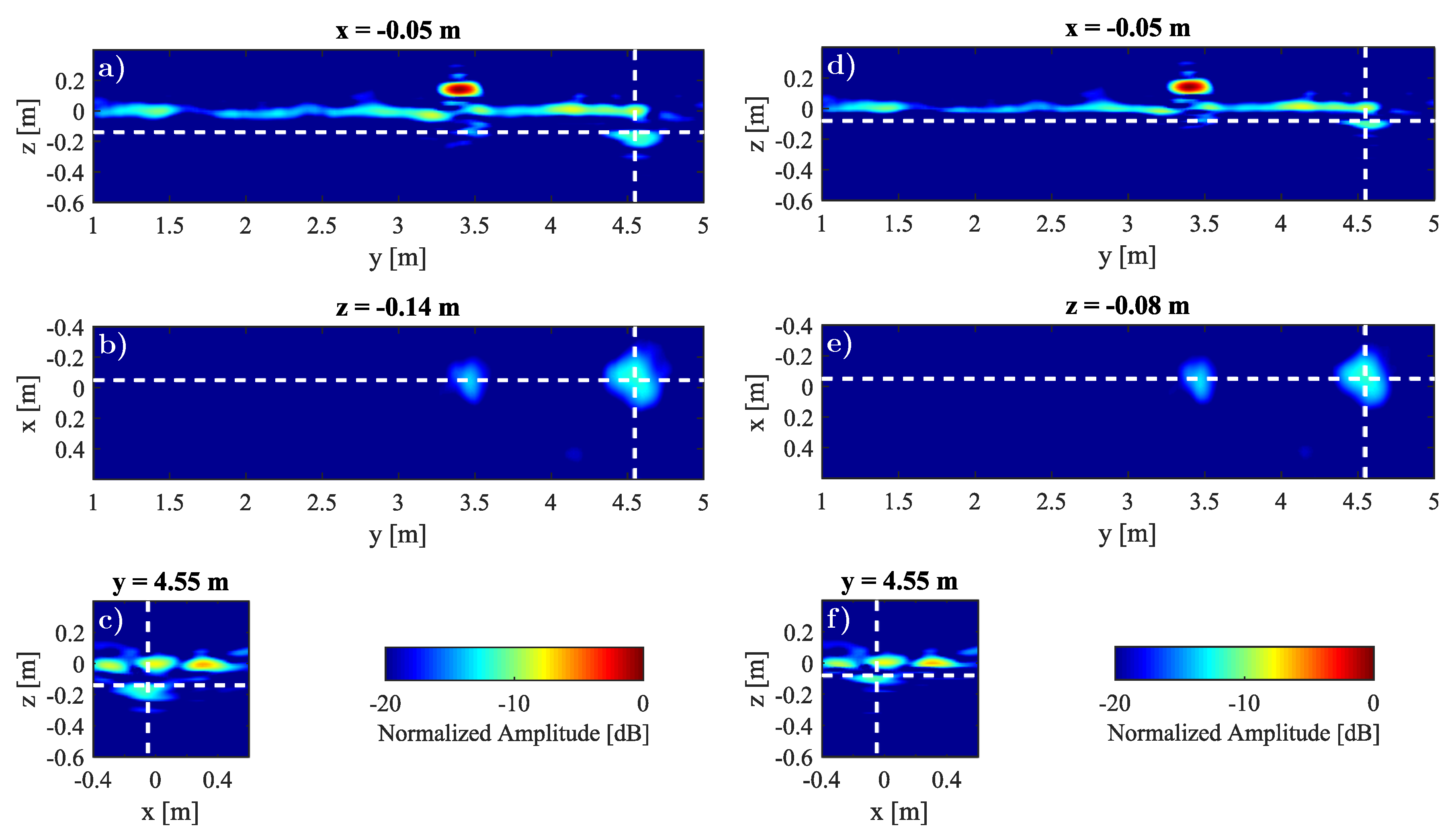
4.2.1. Height Correction

The results obtained applying the height correction described in Section 3.2 are shown on the left part of Figure 17. Comparing them with the results without the height correction (right part of Figure 15), the cylindrical metallic box has become clearly distinguishable from the air–soil interface. Furthermore, the reflection of the air–soil interface has been mitigated thanks to the second background subtraction applied in the height correction step. This mitigation results in less amplitude in the SAR image around $z=0$ m, which is especially evident in the $YZ$ slice (where some areas corresponding to the interface have a normalized amplitude smaller than $-30$ dB). As a result, there is an improvement in the signal to clutter ratio. As a side effect, there is also a considerable amplitude in the SAR image approximately under the metallic disk, which might be due to some secondary reflections.

4.2.2. Equalization

The effect of applying the equalization can be observed comparing the SAR image slices when equalization is applied (right part of Figure 17) with the results of the basic processing (right part of Figure 15). As explained above, the goal of the equalization is to effectively use the whole bandwidth, preventing the low frequency data masking the high frequency one. Thus, the range resolution, which corresponds in this case to the resolution in the z-axis, should improve with the equalization. This improvement is clearly visible since the width of the high reflectivity areas corresponding to the disk, the box and the air–soil interface is narrower. As a result, the buried box can be now distinguished from the air–soil interface.

4.2.3. Height Correction and Equalization

If both height correction and equalization are applied, the resulting SAR image (shown in left part of Figure 18) has better resolution and higher signal to clutter ratio than the one obtained with the basic processing. Furthermore, the equalization also helps to remove the artifact that appears under the metallic disk after applying the height correction. Thus, the combination of these improvements helps to enhance the range resolution (especially the equalization) and the signal to clutter ratio (mainly by reducing the reflection at the air–soil interface with the height correction).

4.2.4. Soil Composition Consideration

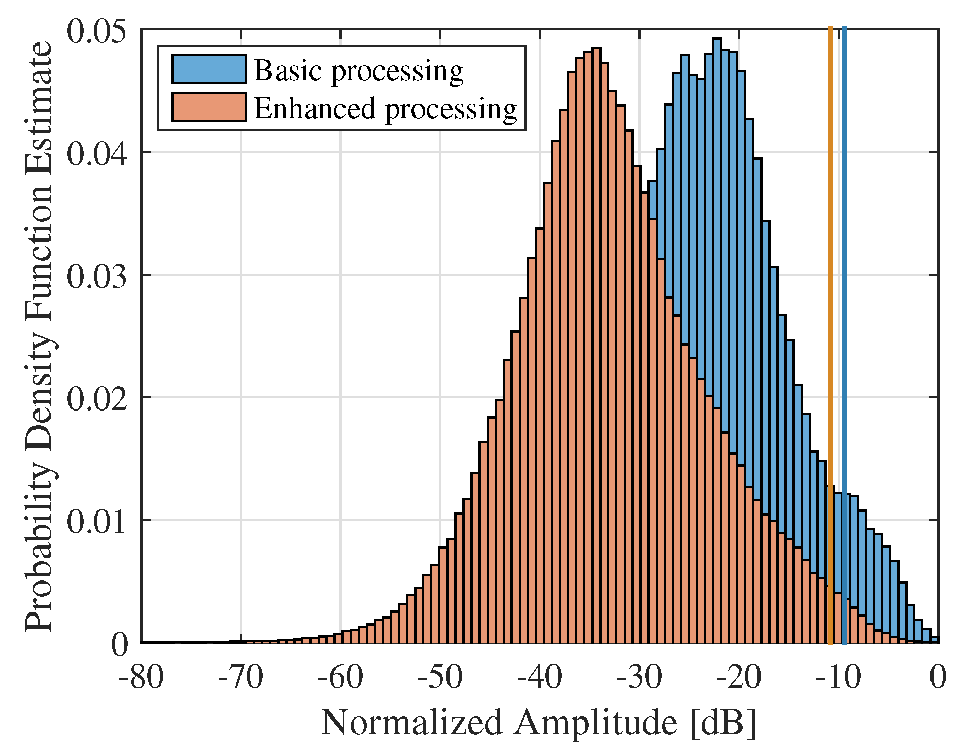
Finally, the soil composition must be taken into account in order to obtain a well-focused SAR image with the buried targets detected at their true depth. Soil permittivity can be estimated from the radar measurements or from the characteristics of the scenario (temperature, soil material components and volumetric water content). A relative permittivity of ${\epsilon }_r=3$ has been assumed, based on previous soil characterization results from [24]. This agrees with the fact that, when free-space propagation is considered, the box is detected at a depth of approximately $d_{box}\sqrt{{\epsilon }_r}=0.14$ m (being $d_{box}=0.08$ m the true depth).

The resulting SAR images are shown in Figure 18b. The box is now detected around its true depth (that is, the depth where the box is detected when it is not covered by soil).

4.3. Comparison

To further compare the results, the histograms of the 3D SAR images amplitudes when using basic and enhanced processing (height correction, equalization and soil composition consideration) are shown in Figure 19 (in blue and orange respectively) for the second measurement (i.e., when there is a buried target). In this figure, the vertical lines indicate the maximum amplitude of the buried target in the corresponding 3D SAR images. This representation allows quantitatively assessing the influence of the proposed enhanced processing. When applying this enhanced processing, the distance between the target amplitude (depicted in the vertical line) and the clutter is increased, which helps to improve the detection capabilities of the system and to reduce the false alarm rate.

5. Conclusions

An enhanced UAV-mounted SAR imaging system to obtain 3D high-resolution radar images (where both underground and overground targets can be detected) is presented. The ultimate goal is the detection of buried hazards, mainly landmines and IEDs, although it can be used for a wide range of application involving both subsurface sensing and terrain observation.

First, several improvements have been implemented in the proposed prototype, mainly to increase the accuracy of the positioning system and the penetration of the electromagnetic waves into the soil. As shown in the results, this allows the coherent combination of measurements gathered at arbitrary positions (3D measurement grid), providing high-resolution radar images, and it also enables the detection of targets buried in higher losses soils.

Concerning the methodology, the processing chain for both the positioning and radar data is thoroughly explained. This methodology can be used to process data collected in both manual and autonomous flight mode, since it selects which measurements will be processed and the location of the investigation domain taking into account the set of UAV positions where measurements were acquired during the flight (i.e., the observation domain). Furthermore, several enhancements in the radar processing are presented to improve the resulting 3D images (mainly in terms of resolution and target discrimination).

Both the prototype and the methodology were experimentally validated with autonomous measurement flights, proving the capability of the system to provide high-resolution 3D SAR images even when using a basic processing strategy. In addition, the effectiveness of the enhanced radar processing was also proved, showing that it yields better resolution and signal to clutter ratio. As expected, results also confirm that, when an estimation of the soil composition is taken into account the buried targets are detected at their true depth.

6. Patents

The work presented in this contribution is related to the patent “Airborne Systems and Detection Methods Localisation and Production of Images of Buried Objects and Characterisation of the Composition of the Subsurface”. Publication No. WO/2017/125627. International Application No. PCT/ES2017/000006. Priority date: 21 January 2016. International filing date: 18 January 2017. University of Oviedo, University of Vigo. Available online: https://patentscope.wipo.int/search/en/detail.jsf?docId=WO2017125627 (accessed on 1 September 2019).

References

1. Yao, H.; Qin, R.; Chen, X. Unmanned Aerial Vehicle for Remote Sensing Applications—A Review. Remote Sens. 2019, 11, 1443. [Google Scholar] [CrossRef]
2. Hildmann, H.; Kovacs, E. Review: Using Unmanned Aerial Vehicles (UAVs) as Mobile Sensing Platforms (MSPs) for Disaster Response, Civil Security and Public Safety. Drones 2019, 3, 59. [Google Scholar] [CrossRef]
3. Manfreda, S.; McCabe, M.F.; Miller, P.E.; Lucas, R.; Pajuelo Madrigal, V.; Mallinis, G.; Ben Dor, E.; Helman, D.; Estes, L.; Ciraolo, G.; et al. On the Use of Unmanned Aerial Systems for Environmental Monitoring. Remote Sens. 2018, 10, 641. [Google Scholar] [CrossRef]
4. Jeziorska, J. UAs for Wetland Mapping and Hydrological Modeling. Remote Sens. 2019, 11, 1997. [Google Scholar] [CrossRef]
5. Garcia-Fernandez, M.; Alvarez-Lopez, Y.; Las Heras, F. On the use of Unmanned Aerial Vehicles for antenna and coverage diagnostics in mobile networks. IEEE Commun. Mag. 2018, 56, 72–78. [Google Scholar] [CrossRef]
6. Llort, M.; Aguasca, A.; Lopez-Martinez, C.; Martinez-Marin, T. Initial evaluation of SAR capabilities in UAV multicopter platforms. IEEE J. Sel. Top. Appl. Earth Obs. Remote Sens. 2018, 11, 127–140. [Google Scholar] [CrossRef]
7. Garcia-Fernandez, M.; Alvarez-Lopez, Y.; Arboleya-Arboleya, A.; Gonzalez-Valdes, B.; Rodriguez-Vaqueiro, Y.; Las Heras, F.; Pino, A. Synthetic Aperture Radar imaging system for landmine detection using a Ground Penetrating Radar on board an Unmanned Aerial Vehicle. IEEE Access 2018, 6, 45100–45112. [Google Scholar] [CrossRef]
8. Robledo, L.; Carrasco, M.; Mery, D. A survey of land mine detection technology. Int. J. Remote Sens. 2009, 30, 2399–2410. [Google Scholar] [CrossRef]
9. Jol, H.M. Ground Penetrating Radar Theory and Applications; Elsevier Science: Amsterdam, The Netherlands, 2009. [Google Scholar]
10. Daniels, D.J. A review of GPR for landmine detection. Sens. Imaging Int. J. 2006, 7, 90–123. [Google Scholar] [CrossRef]
11. Rappaport, C.; El-Shenawee, M.; Zhan, H. Suppressing GPR clutter from randomly rough ground surfaces to enhance nonmetallic mine detection. Subsurf. Sens. Technol. Appl. 2003, 4, 311–326. [Google Scholar] [CrossRef]
12. Wang, T.; Keller, J.M.; Gader, P.D.; Sjahputera, O. Frequency subband processing and feature analysis of forward-looking ground-penetrating radar signals for land-mine detection. IEEE Trans. Geosci. Remote Sens. 2007, 45, 718–729. [Google Scholar] [CrossRef]
13. Peichl, M.; Schreiber, E.; Heinzel, A.; Kempf, T. TIRAMI-SAR—A Synthetic Aperture Radar approach for efficient detection of landmines and UXO. In Proceedings of the 10th European Conference on Synthetic Aperture Radar—EuSAR, Berlin, Germany, 3–5 June 2014. [Google Scholar]
14. Comite, D.; Galli, A.; Catapano, I.; Soldovieri, F. Advanced imaging for down-looking contactless GPR systems. In Proceedings of the International Applied Computational Electromagnetics Society Symposium—Italy (ACES), Florence, Italy, 26–30 March 2017. [Google Scholar]
15. Gonzalez-Valdes, B.; Alvarez-Lopez, Y.; Arboleya, A.; Rodriguez-Vaqueiro, Y.; Garcia-Fernandez, M.; Las Heras, F.; Pino, A. Airborne Systems and Methods for the Detection, Localisation and Imaging of Buried Objects, and Characterization of the Subsurface Composition. ES Patent 2,577,403 (WO2017/125627), 21 January 2016. [Google Scholar]
16. Fasano, G.; Renga, A.; Vetrella, A.R.; Ludeno, G.; Catapano, I.; Soldovieri, F. Proof of concept of micro-UAV-based radar imaging. In Proceedings of the International Conference on Unmanned Aircraft Systems (ICUAS), Miami, FL, USA, 13–16 June 2017. [Google Scholar]
17. Schartel, M.; Bähnemann, R.; Burr, R.; Mayer, W.; Waldschmidt, C. Position acquisition for a multicopter-based synthetic aperture radar. In Proceedings of the 20th International Radar Symposium (IRS), Ulm, Germany, 26–28 June 2019. [Google Scholar]
18. Alvarez-Narciandi, G.; Lopez-Portuges, M.; Las-Heras, F.; Laviada, J. Freehand, Agile and High-Resolution Imaging With Compact mm-Wave Radar. IEEE Access 2019, 7, 95516–95526. [Google Scholar] [CrossRef]
19. Gonzalez-Diaz, M.; Garcia-Fernandez, M.; Alvarez-Lopez, Y.; Las Heras, F. Improvement of GPR SAR-based techniques for accurate detection and imaging of buried objects. IEEE Trans. Instrum. Meas. 2019. [Google Scholar] [CrossRef]
20. Topcon B111 Receiver. Available online: https://www.topconpositioning.com/oem-components-technology/gnss-components/b111 (accessed on 31 August 2019).
21. Solimene, R.; Cuccaro, A.; Dell’Aversano, A.; Catapano, I.; Soldovieri, F. Ground clutter removal in gpr surveys. IEEE J. Sel. Top. Appl. Earth Obs. Remote Sens. 2014, 7, 792–798. [Google Scholar] [CrossRef]
22. Johansson, E.M.; Mast, J.E. Three-dimensional ground-penetrating radar imaging using synthetic aperture time-domain focusing. In Proceedings of the International Symposium on Optics, Imaging, and Instrumentation, International Society for Optics and Photonics, San Diego, CA, USA, 14 September 1994. [Google Scholar]
23. Fuse, Y.; Gonzalez-Valdes, B.; Martinez-Lorenzo, J.A.; Rappaport, C.M. Advanced SAR imaging methods for forward-looking ground penetrating radar. In Proceedings of the European Conference on Antennas and Propagation, Davos, Switzerland, 10–15 April 2016. [Google Scholar]
24. Alvarez, Y.; Garcia-Fernandez, M.; Arboleya-Arboleya, A.; Gonzalez-Valdes, B.; Rodriguez-Vaqueiro, Y.; Las-Heras, F.; Pino, A. SAR-based technique for soil permittivity estimation. Int. J. Remote Sens. 2017, 38, 5168–5186. [Google Scholar] [CrossRef]
Figure 1. UAV-mounted GPR prototype.
Remotesensing 11 02357 g001
Figure 2. Flowchart of the data processing.
Remotesensing 11 02357 g002
Figure 3. Histogram of the course over the ground.
Remotesensing 11 02357 g003
Figure 4. Original and rotated flight path (in blue and red, respectively).
Remotesensing 11 02357 g004
Figure 5. One of each four consecutive UAV positions (a); full and selected UAV positions (in blue and red, respectively) (b); and one of each four consecutive selective UAV positions (c).
Remotesensing 11 02357 g005
Figure 6. Definition of the investigation plane edges (in solid red line) from the observation plane coordinates (in dotted blue line).
Remotesensing 11 02357 g006
Figure 7. Normalized radar measurements ( E s c a t t ( r n g ) ) after time-zero correction and time-window selection. The distance between the radar antennas and the soil is depicted in black on top of the measurement.
Remotesensing 11 02357 g007
Figure 8. Normalized radar measurements ( E ˜ s c a t t ( r n g ) ) after background subtraction. The distance between the radar antennas and the soil is depicted in white on top of the measurement.
Remotesensing 11 02357 g008
Figure 9. Closer look to the radar measurements before (a) and after (b) background subtraction.
Remotesensing 11 02357 g009
Figure 10. Normalized radar measurement ( E ^ s c a t t ( r n g ) ) after height shifting.
Remotesensing 11 02357 g010
Figure 11. Closer look to the radar measurement ( E ^ s c a t t ( r n g ) ) after height shifting.
Remotesensing 11 02357 g011
Figure 12. Main parameters involved in the estimation of the path length when the soil permittivity is taken into account (dashed line represents the true ray path).
Remotesensing 11 02357 g012
Figure 13. Measurement scenario.
Remotesensing 11 02357 g013
Figure 14. Setup for the measurement (a); first with the 9.5 cm radius metallic box uncovered (b); and second with this box buried and covered with soil (c).
Remotesensing 11 02357 g014
Figure 15. Slices of the 3D SAR image at the position where the buried metallic cylindrical box is detected. Results for the the first measurement (uncovered buried metallic box) are depicted on the left: along-track view at x = 0.05 m (a); top view at z = 0.08 m (b); and across-track view at y = 4.55 m (c). Results for the the second measurement (buried metallic box covered with soil) are depicted on the right: along-track view at x = 0.05 m (d); top view at z = 0.14 m (e); and across-track view at y = 4.55 m (f).
Remotesensing 11 02357 g015
Figure 16. Slices of the 3D SAR image for the second measurement at the position where the cylindrical disk on top of a briefcase is detected (along-track view at x = 0.075 m (a); top view at z = 0.14 m (b); and across-track view at y = 3.4 m (c)) and at a position at the soil surface interface without targets (along-track view at x = 0.3 m (d); top view at z = 0 m (e); and across-track view at y = 2 m (f)).
Remotesensing 11 02357 g016
Figure 17. Slices of the 3D SAR image at the position where the cylindrical box is detected when height correction is applied (on the left) and when the SAR image is equalized (on the right): (a,d) along-track views at x = 0.05 m; (b,e) top views at z = 0.14 m; and (c,f) across-track views at y = 4.55 m.
Remotesensing 11 02357 g017
Figure 18. Slices of the 3D SAR image at the position where the cylindrical box is detected when height correction and equalization are applied. Results on the left are obtained without taking into account the soil composition, whereas results on the right are obtained assuming ε r = 3 : (a,d) along-track views at x = 0.05 m; (b,e) top views at z = 0.14 m and z = 0.08 m, respectively; and (c,f) across-track views.
Remotesensing 11 02357 g018
Figure 19. Histograms of the 3D SAR images amplitudes of the second measurement when using basic and enhanced processing (height correction, equalization and soil composition consideration). Vertical lines indicate the maximum amplitude of the buried target in the corresponding 3D SAR images.
Remotesensing 11 02357 g019