Volatility Spillovers and Causality of Carbon Emissions, Oil and Coal Spot and Futures for the EU and USA

Abstract

Recent research shows that the efforts to limit climate change should focus on reducing the emissions of carbon dioxide over other greenhouse gases or air pollutants. Many countries are paying substantial attention to carbon emissions to improve air quality and public health. The largest source of carbon emissions from human activities in some countries in Europe and elsewhere is from burning fossil fuels for electricity, heat, and transportation. The prices of fuel and carbon emissions can influence each other. Owing to the importance of carbon emissions and their connection to fossil fuels, and the possibility of Granger causality in spot and futures prices, returns, and volatility of carbon emissions, crude oil and coal have recently become very important research topics. For the USA, daily spot and futures prices are available for crude oil and coal, but there are no daily futures prices for carbon emissions. For the European Union (EU), there are no daily spot prices for coal or carbon emissions, but there are daily futures prices for crude oil, coal and carbon emissions. For this reason, daily prices will be used to analyse Granger causality and volatility spillovers in spot and futures prices of carbon emissions, crude oil, and coal. As the estimators are based on quasi-maximum likelihood estimators (QMLE) under the incorrect assumption of a normal distribution, we modify the likelihood ratio (LR) test to a quasi-likelihood ratio test (QLR) to test the multivariate conditional volatility Diagonal BEKK model, which estimates and tests volatility spillovers, and has valid regularity conditions and asymptotic properties, against the alternative Full BEKK model, which also estimates volatility spillovers, but has valid regularity conditions and asymptotic properties only under the null hypothesis of zero off-diagonal elements. Dynamic hedging strategies by using optimal hedge ratios are suggested to analyse market fluctuations in the spot and futures returns and volatility of carbon emissions, crude oil, and coal prices.

1. Introduction

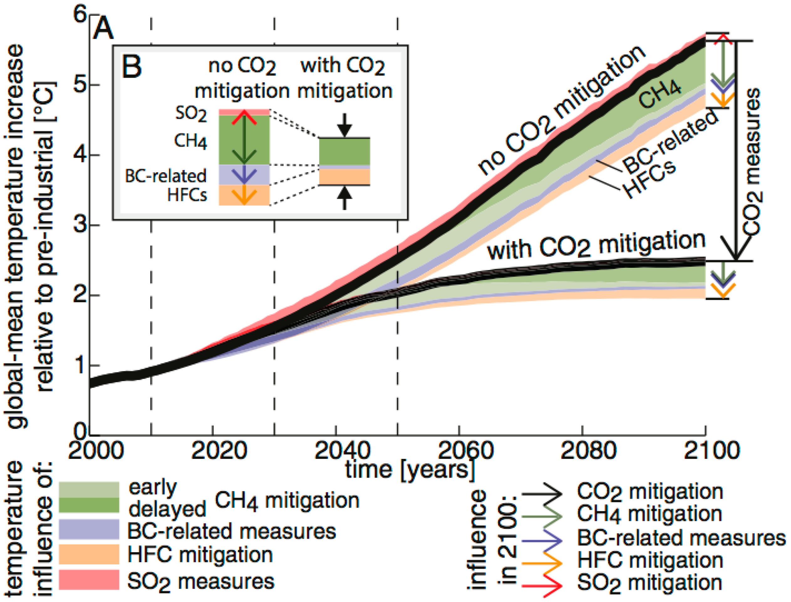
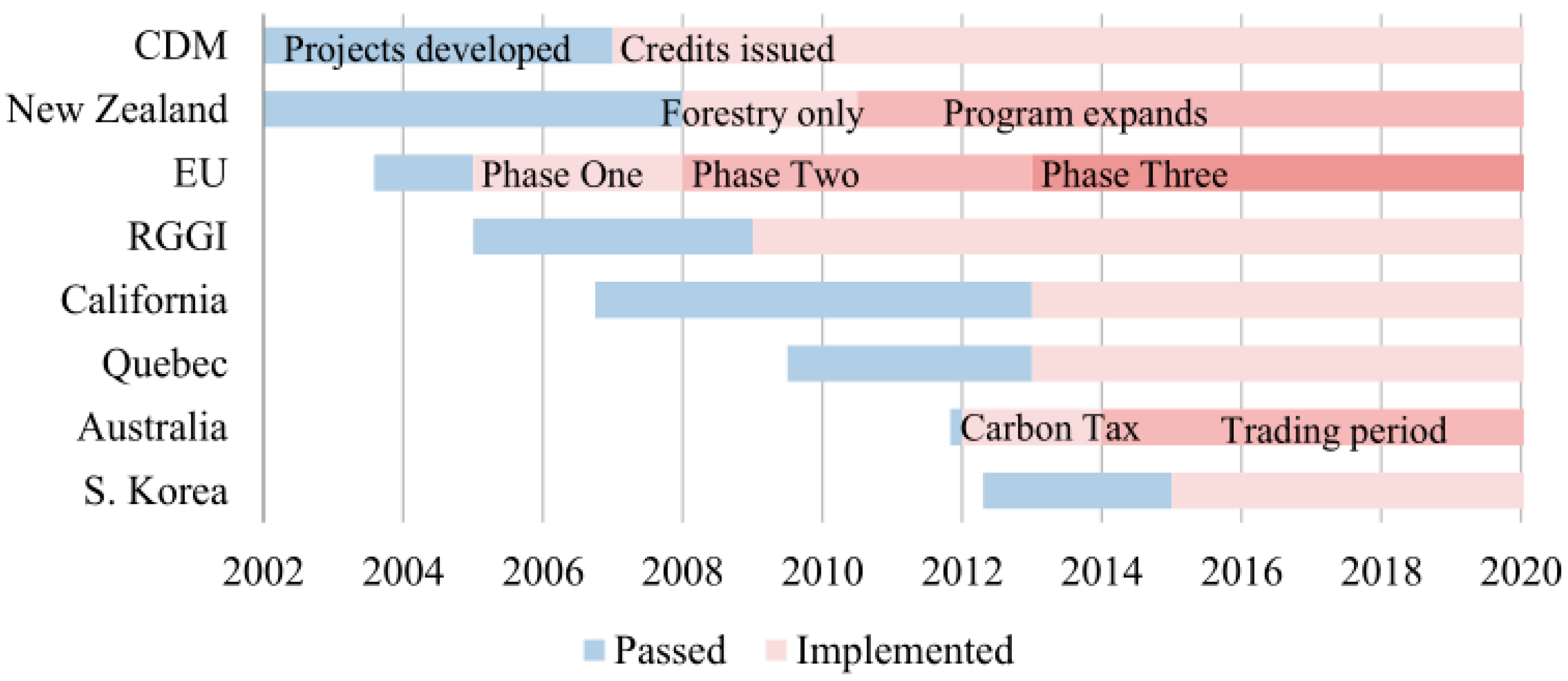
Recent research shows that efforts to limit climate change should focus on reducing emissions of carbon dioxide over other greenhouse gases or air pollutants. Many countries are paying substantially greater attention to carbon emissions to improve air quality and public health. Carbon emissions trading programs have been established at the international, regional, national, and sub-national levels (see Figure 1).

As can be seen from Figure 1, in a scenario of ‘no carbon dioxide mitigation’, global temperatures would be predicted to rise by over five degrees Celsius by 2100, but cutting emissions of methane, HFCs, and black carbon would reduce this rise to around one degree Celsius. The results suggest that carbon dioxide should certainly remain central to greenhouse gas emission cuts.

Figure 2 shows that projects and regions such as the CDM (Clean Development Mechanism), RGGI (Regional Greenhouse Gas Initiative), and European Union (EU), countries like New Zealand, Australia, and South Korea, the State of California in the USA, and the Province of Quebec inn Canada, have passed and implemented programs to mitigate carbon emissions.

The programs have operated in phases, with a pilot phase from 2005 to 2007 covering the power sector and certain heavy industries, a second phase from 2008 to 2012 expanding coverage slightly, and a third phase for 2013–2020 that adds a significant range of industrial activities.

The largest source of carbon emissions from human activities in some countries in Europe and elsewhere is from burning fossil fuels for electricity, heat, and transportation. The price of fuel influences carbon emissions, but the price of carbon emissions can also influence the price of fuel.

Owing to the importance of carbon emissions and their connection to fossil fuels, and the possibility of [2] Granger (1980) causality in spot and futures prices, returns and volatility of carbon emissions, it is not surprising that crude oil and coal have recently become a very important public policy issue, and hence also a significant research topic.

Energy markets have recently expanded considerably due in large part to the rapidly accelerating behaviour of investors in financial markets. The synergy between financial and energy markets is that the financial aspect of fossil fuels and carbon emissions need to be analysed more carefully by using advanced financial econometric methods. An important reference in the field of energy prices and its consequences on financial markets are the empirical studies presented in [3] Ramos and Veiga (2014). These macroeconomic variables include risk factors in the oil industry, risk taking in the airline industry, prices, volatility, and shocks in the oil industry, oil shock spillovers to stock market returns, equity returns, bond returns, and volatility market risks.

In a more microeconomic context, [4] Sawik, Faulin and Pérez-Bernabeu (2017a) examine energy and environment issues with respect to multi-criteria analysis and multi-objective green logistics optimization. The optimality criteria are presented in terms of environmental costs, that is, the minimization of externality costs for noise, pollution, and fuel costs as compared with their minimization. In a separate contribution, [5] Sawik, Faulin and Pérez-Bernabeu (2017b) solve a multi-objective formulation problem by minimizing the total distance, and hence the costs to a delivery company, and the amount of CO₂ emissions. [6] Sawik, Faulin and Pérez-Bernabeu (2017c) optimize a multi-criteria formulation for green vehicle routing problems by mixed integer programming, specifically to decide the best delivery route to minimize the travel costs and optimize the transportation route of a delivery company.

The plan of the remainder of the paper is as follows. Section 2 discusses the spot and futures data for carbon emissions, coal, and oil that will be used in the empirical analysis for the EU and USA. Section 3 discusses methodological issues, including univariate and multivariate conditional volatility models, Granger causality, volatility spillovers, optimal hedge ratios, causality in returns and volatility, as well as an interesting and novel adaptation of the likelihood ratio (LR) test to a quasi likelihood ratio (QLR) test of the Diagonal BEKK model against the alternative of a Full BEKK model. Section 4 examines the alternative unit root tests that are used to test for stationarity in the data. Granger Causality and Spillovers in Returns and Volatilities are analysed in Section 5. Section 6 provides some concluding remarks.

2. Data

The length of the sample period for the empirical analysis was dictated by the availability of data on carbon, coal, and crude oil spot and futures prices in the EU and the United States of America (USA). The carbon emission trading market of the EU has the longest trading period for futures prices, but not for spot prices. The USA is the leader in developing a wide range of financial derivatives, such as futures prices, for financial, energy, and commodities, but not for carbon emissions, where only spot prices are available.

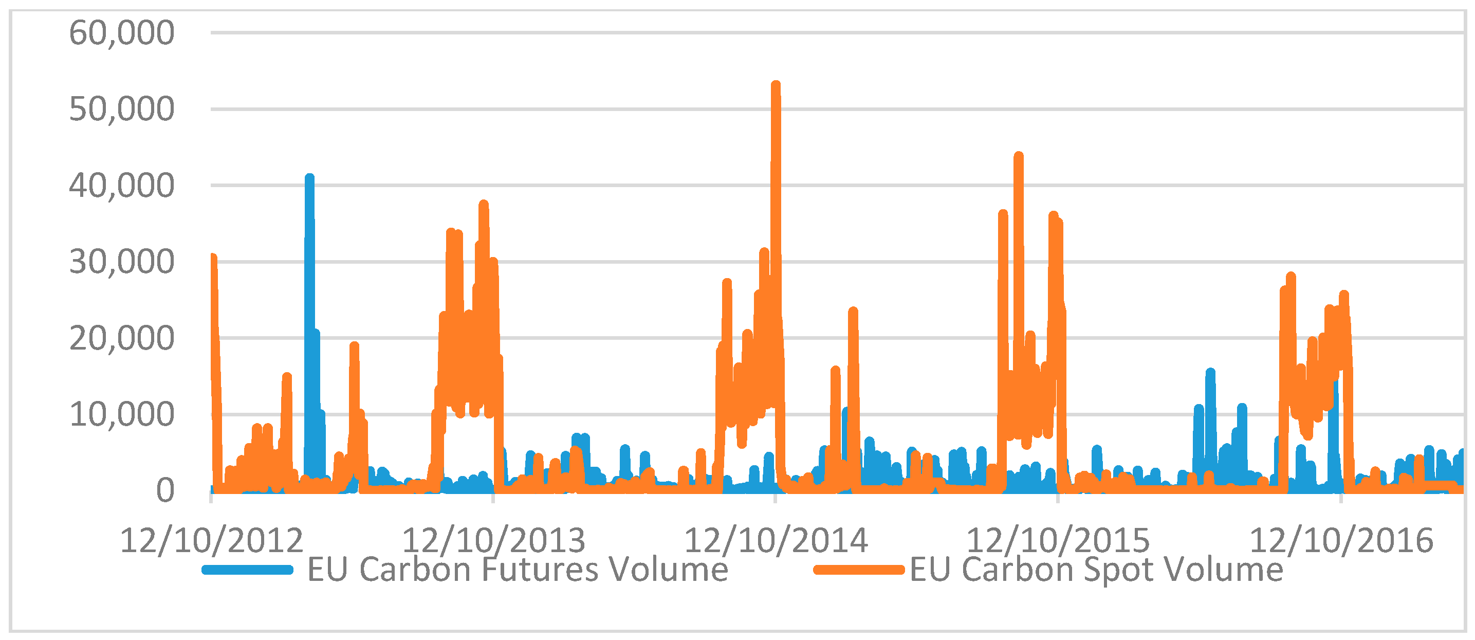
Data for EU carbon emission, crude oil, and coal futures are available from 1 April 2008 to 20 May 2017, and these will be analyzed in the paper. Coal spot price in the EU is available on a weekly basis. The spot prices of carbon emission and crude oil have a high correlation with the corresponding futures prices. The volume of trades in the spot market of carbon emissions is much smaller than in the futures market, as shown in Figure 3.

Data for crude oil are available prior to 2000. However, the data for the spot prices of coal and carbon emissions start from 17 July 2006 and 1 April 2008, respectively. Therefore, the data in the empirical analysis for the European Union starts from the latest date for crude oil, coal, and carbon emissions, namely 1 April 2008.

Data for carbon, coal, and oil spot prices from 5 January 2016 to 20 May 2017 for the USA will also be analyzed in the paper, but data for futures prices of carbon emissions are not available for the USA. Spot prices for coal and crude oil start prior to 2000. However, data for carbon emissions start from 1 May 2016. Consequently, the spot price data in the empirical analysis for the USA starts from the latest date for oil, coal, and carbon emissions, namely 5 January 2016.

The transaction markets and units for the variables are different. EU carbon futures is the Intercontinental Exchange EU allowance, which is traded in the ICE-ICE Futures Europe Commodities market and is expressed in Euros per metric ton. EU coal futures is ICE Rotterdam Monthly Coal Futures Contract, and is traded in the ICE-ICE Futures Europe Commodities market. EU oil futures is the current pipeline export quality Brent blend, as supplied at Sullom Voe, is traded in the ICE-ICE Futures Europe Commodities market, and is expressed in USDs per bbl.

Carbon spot prices in the USA are given as the United States Carbon Dioxide RGGI Allowance, and are expressed in USDs per allowance. Coal spot prices are given as the Dow Jones US Total Market Coal Index, which is expressed in USD. Oil spot returns are given as the West Texas Intermediate Cushing Crude Oil, which is expressed in USDs per bbl. All of the currency units are transformed to USD in the empirical analysis.

The endogenous variables used in the empirical analysis are daily returns, where the rate of return is obtained as the first difference in the natural logarithm of the relevant daily price data. The mnemonics ${\mathrm{EUcarbon}}_{\mathrm{fr}},$ ${\mathrm{EUcoal}}_{\mathrm{fr}},$ ${\mathrm{EUoil}}_{\mathrm{fr}}$ denote, respectively, the future returns of carbon emission, coal, and oil in the European Union. Similarly, the mnemonics ${\mathrm{UScarbon}}_{\mathrm{sr}},{ \mathrm{UScoal}}_{\mathrm{sr}},{ \mathrm{USoil}}_{\mathrm{sr}}$ denote, respectively, the spot returns for carbon emission, coal, and oil in the USA.

The variable sources and definitions are given in

Table 1. Data Sources and Definitions.

Variable Name	Definitions	Transaction Market	Description
${\mathrm{EUcarbon}}_{\mathrm{fr}}$	EU carbon futures return	ICE-ICE Futures Europe Commodities	ICE EUA Futures Contract EUR/MT
${\mathrm{EUcoal}}_{\mathrm{fr}}$	EU coal futures return	ICE-ICE Futures Europe Commodities	ICE Rotterdam Monthly Coal Futures Contract USD/MT
${\mathrm{EUoil}}_{\mathrm{fr}}$	EU oil futures return	ICE-ICE Futures Europe Commodities	Current pipeline export quality Brent blend as supplied at Sullom Voe USD/bbl
${\mathrm{UScarbon}}_{\mathrm{sr}}$	US carbon spot return	over the counter	United States Carbon Dioxide RGGI Allowance USD/Allowance
${\mathrm{UScoal}}_{\mathrm{sr}}$	US coal spot return	over the counter	Dow Jones US Total Market Coal Index USD
${\mathrm{USoil}}_{\mathrm{sr}}$	US oil spot return	over the counter	West Texas Intermediate Cushing Crude Oil USD/bbl

ICE is the Intercontinental Exchange; EUA is the EU allowance; MT is metric ton; RGGI (Regional Greenhouse Gas Initiative) is a CO₂ cap-and-trade emissions trading program that is comprised of ten New England and Mid-Atlantic States that will commence in 2009 and aims to reduce emissions from the power sector. RGGI will be the first government mandated CO₂ emissions trading program in USA.

, with respect to the futures returns for the EU and spot returns for the USA, as well as their transactions markets, and the descriptions of the data.

For the USA, daily spot and futures prices are available for crude oil and coal, but there are no daily spot or futures prices for carbon emissions. For the EU, there are no daily spot prices for coal or carbon emissions, but there are daily futures prices for crude oil, coal, and carbon emissions.

For this reason, daily futures prices will be used to analyse Granger causality and volatility spillovers in spot and futures prices of carbon emissions, crude oil, and coal. This will be based on the Lagrange multiplier test of univariate causality in variance (strictly, causality in conditional volatility) of [7] Hafner and Herwartz (2006), and more recently, [8] Chang and McAleer (2017). An extension to multivariate tests of causality in conditional volatility will be a focus of the paper.

As the estimators are based on Quasi-Maximum Likelihood Estimators (QMLE) under the incorrect assumption of a normal likelihood function, we will modify the likelihood ratio (LR) test to a novel quasi-likelihood ratio test (QLR).

Definition of QLR test statistic: QLR = 2 (quasi maximized log likelihood value under the alternative hypothesis − quasi maximized log likelihood value under the null hypothesis).

The QLR test statistic tests the multivariate conditional volatility Diagonal BEKK model, which is used to estimate and test spillovers, and which has valid regularity conditions and asymptotic properties, against the alternative Full BEKK model, which is used to estimate spillovers, but has valid regularity conditions and asymptotic properties only under the null hypothesis of zero off-diagonal elements. Dynamic hedging strategies using optimal hedge ratios will be suggested to analyse market fluctuations in the spot and futures returns and volatility of carbon emissions, crude oil, and coal prices.

The QLR statistic has an asymptotic chi-squared distribution under the null hypothesis, with degrees of freedom (df) equivalent to the number of off-diagonal terms in the two m × m matrices, the weighting matrix, A, and the stability matrix, B, of the Full BEKK model, namely 2m(m − 1).

The descriptive statistics for the endogenous returns of the variables are given in

Table 2. Descriptive Statistics 2 April 2008–19 May 2017 for EU 6 January 2016–19 May 2017 for United States of America (USA).

Variable	Mean	Median	Max	Min	SD	Skewness	Kurtosis	Jarque-Bera
$EUcarbo{n}_{fr}$	−0.078	−0.038	24.561	−42.457	3.349	−0.708	17.624	21,434.2
$EUcoa{l}_{fr}$	−0.022	0	17.419	−22.859	1.599	−1.268	44.924	175,155.8
$EUoi{l}_{fr}$	−0.026	−0.015	12.707	−10.946	2.246	0.054	6.522	1232.8
$UScarbo{n}_{sr}$	−0.248	0	13.937	−36.446	2.986	−5.236	66.269	61,346.8
$UScoa{l}_{sr}$	0.177	0.104	17.458	−14.183	4.041	0.047	5.343	81.99
$USoi{l}_{sr}$	0.094	0.037	11.621	−8.763	2.712	0.431	4.690	53.69

The Jarque-Bera Lagrange multiplier statistic for normality is based on testing the empirical skewness and kurtosis against their normal counterparts.

. The highest standard deviation for the EU over the sample period is for carbon futures, followed by oil and coal futures. Similarly, the highest standard deviation for the US market is for coal spot returns, followed by carbon emission spot returns.

The returns have different degrees of skewness. The futures and spot returns of oil in the EU and US markets, and coal spot returns in the USA are skewed to the left, indicating that these series have longer left tails (extreme losses) than right tails (extreme gains). However, other returns are all skewed to the right, especially carbon emission spot return in the USA, for which the value of the skewness is high, indicating that these series have more extreme gains than extreme losses.

These stylized facts should be of interest to participants in commodity markets. All of the price distributions have kurtosis that is significantly higher than three, implying that higher probabilities of extreme market movements in either direction (gains or losses) occur in these futures markets, with greater frequency in practice than would be expected under the normal distribution.

In the EU market, the highest kurtosis is for coal futures, followed by carbon futures and oil futures. For the US market, the highest kurtosis is for carbon spot, followed by coal spot. The Jarque-Bera Lagrange multiplier statistic is based on testing the empirical skewness and kurtosis against their normal counterparts, and confirms the non-normal distributions for all of the returns series.

3. Methodology

Although financial and energy returns are almost certainly stationary, the empirical analysis will commence with tests of unit roots based on ADF, DF-GLS, and KPSS. This will be followed by an analysis and estimation of univariate GARCH and multivariate diagonal BEKK models (see [9] Baba et al. (1985) [10] Engle and Kroner (1995)), from which the conditional covariances will be used for testing co-volatility spillovers, that is, Granger causality in conditional volatility.

Despite the empirical applications of a wide range of conditional volatility models in numerous papers in empirical finance, there are theoretical problems associated with virtually all of them. The CCC ([11] Bollerslev (1990)), VARMA-GARCH ([12] Ling and McAleer (2003), and its asymmetric counterpart, VARMA-AGARCH [13] McAleer et al. (2009)), models have static conditional covariances and correlations, which means that accommodating volatility spillovers is not possible.

Apart from the diagonal version, the multivariate Full BEKK model of conditional covariances has been shown to have no regularity conditions, and hence no statistical properties (see [14] McAleer et al. (2008) and [15] Chang and McAleer (2017b), and the discussion below, for further details). Therefore, spillovers can be considered only for the special case of Diagonal BEKK. The multivariate DCC model of (purported) conditional correlations has been shown to have no regularity conditions, and hence no statistical properties (see [16] Hafner and McAleer (2014) and [17] McAleer (2017) for further details).

The analysis of univariate and multivariate conditional volatility models below is a summary of what has been presented in the literature (see, for example [18] Caporin and McAleer (2012) [19] Chang et al. (2015), and especially [20] Chang et al. (2017)), although a comprehensive discussion of the Full and Diagonal BEKK models is not available in any published source. In particular, the application of the quasi likelihood ratio (QLR) test of the Diagonal BEKK model as the null hypothesis against the alternative hypothesis of a Full BEKK model does not seem to have been considered in the literature.

The first step in estimating multivariate models is to obtain the standardized residuals from the conditional mean returns shocks. For this reason, the most widely used univariate conditional volatility model, namely GARCH, will be presented briefly, followed by the two most widely estimated multivariate conditional covariance models, namely the Diagonal and Full BEKK models.

3.1. Univariate Conditional Volatility

Consider the conditional mean of financial returns, as follows:

$$y_t=E\left(y_t|I_{t-1}\right)+{\epsilon }_t$$

(1)

where the financial returns, $y_t=\Delta log{P}_t$, represent the log-difference in the financial commodity or agricultural prices, $P_t$, $I_{t-1}$ is the information set at time t − 1, and ${\epsilon }_t$ is a conditionally heteroskedastic error term, or returns shock. In order to derive conditional volatility specifications, it is necessary to specify the stochastic processes underlying the returns shocks, ${\epsilon }_t$. The most popular univariate conditional volatility model, GARCH model, is discussed below.

Now consider the random coefficient AR (1) process underlying the return shocks, ${\epsilon }_t$:

$${\epsilon }_t={\varphi }_t{\epsilon }_{t-1}+{\eta }_t$$

(2)

where ${\varphi }_t~iid\left(0,\alpha \right),$ $\alpha$≥ 0, ${\eta }_t~iid\left(0,\omega \right),$ $\omega$≥ 0, ${\eta }_t={\epsilon }_t/\sqrt{h_t}$ is the standardized residual, with $h_t$ defined below.

[21] Tsay (1987) derived the ARCH (1) model of [22] Engle (1982) and [23] Bollerslev (1986) from Equation (2) as:

$$h_t\equiv E({\epsilon }_t^2|I_{t-1})=\omega +\alpha {\epsilon }_{t-1}^2$$

(3)

where $h_t$ represents conditional volatility, and $I_{t-1}$ is the information set available at time t − 1. A lagged dependent variable, $h_{t-1}$, is typically added to Equation (3) to improve the sample fit:

$$h_t\equiv E({\epsilon }_t^2|I_{t-1})=\omega +\alpha {\epsilon }_{t-1}^2+\beta h_{t-1}$$

(4)

From the specification of Equation (2), it is clear that both $\omega$ and $\alpha$ should be positive, as they are the unconditional variances of two different stochastic processes.

Given the non-normality of the returns shocks, the Quasi-Maximum Likelihood Estimators (QMLE) of the parameters have been shown to be consistent and asymptotically normal in several papers. For example [12] Ling and McAleer (2003) showed that the QMLE for a generalized ARCH(p,q) (or GARCH(p,q)) is consistent if the second moment is finite. A sufficient condition for the QMLE of GARCH(1,1) in Equation (4) to be consistent and asymptotically normal is $\alpha +\beta <1$.

In general, the proofs of the asymptotic properties follow from the fact that GARCH can be derived from a random coefficient autoregressive process. Ref. [13] McAleer et al. (2008) give a general proof of asymptotic normality for multivariate models that are based on proving that the regularity conditions satisfy the conditions given in [24] Jeantheau (1998) for consistency, and the conditions given in Theorem 4.1.3 in [25] Amemiya (1985) for asymptotic normality.

3.2. Multivariate Conditional Volatility

The multivariate extension of the univariate ARCH and GARCH models is given in [9] Baba et al. (1985) and [10] Engle and Kroner (1995) (for caveats regarding Full BEKK, see [15] Chang and McAleer (2017b)). In order to establish volatility spillovers in a multivariate framework, it is useful to define the multivariate extension of the relationship between the returns shocks and the standardized residuals, that is, ${\eta }_t={\epsilon }_t/\sqrt{h_t}$.

The multivariate extension of Equation (1), namely $y_t=E(y_t|I_{t-1})+{\epsilon }_t$, can remain unchanged by assuming that the three components are now $m\times 1$ vectors, where $m$ is the number of financial assets. The multivariate definition of the relationship between ${\epsilon }_t$ and ${\eta }_t$ is given as:

$${\epsilon }_t=D_t^{1/2}{\eta }_t$$

(5)

where $D_t=diag\left(h_{1t},h_{2t},\dots ,h_{mt}\right)$ is a diagonal matrix comprising the univariate conditional volatilities.

Define the conditional covariance matrix of ${\epsilon }_t$ as $Q_t$. As the $m\times 1$ vector, ${\eta }_t$, is assumed to be iid for all $m$ elements, the conditional correlation matrix of ${\epsilon }_t$, which is equivalent to the conditional correlation matrix of ${\eta }_t$, is given by ${\Gamma }_t$. Therefore, the conditional expectation of (5) is defined as:

$$Q_t=D_t^{1/2}{\Gamma }_t{D}_t^{1/2}$$

(6)

Equivalently, the conditional correlation matrix, ${\Gamma }_t$, can be defined as:

$${\Gamma }_t=D_t^{-1/2}{Q}_t{D}_t^{-1/2}.$$

(7)

Equation (6) is useful if a model of ${\Gamma }_t$ is available for purposes of estimating $Q_t$, whereas (7) is useful if a model of $Q_t$ is available for the purposes of estimating ${\Gamma }_t$.

Equation (6) is convenient for a discussion of volatility spillover effects, while both Equations (6) and (7) are instructive for a discussion of asymptotic properties. As the elements of $D_t$ are consistent and asymptotically normal, the consistency of $Q_t$ in (6) depends on the consistent estimation of ${\Gamma }_t$, whereas the consistency of ${\Gamma }_t$ in (7) depends on the consistent estimation of $Q_t$. As both $Q_t$ and ${\Gamma }_t$ are products of matrices, with inverses in (7), neither the QMLE of $Q_t$ nor ${\Gamma }_t$ will be asymptotically normal based on the definitions given in Equations (6) and (7).

3.3. Diagonal BEKK

The Diagonal BEKK model can be derived from a vector random coefficient autoregressive process of order one, which is the multivariate extension of the univariate process given in Equation (2):

$${\epsilon }_t={\Phi }_t{\epsilon }_{t-1}+{\eta }_t$$

(8)

where ${\epsilon }_t$ and ${\eta }_t$ are $m\times 1$ vectors, ${\Phi }_t$ is an $m\times m$ matrix of random coefficients, ${\Phi }_t~iid\left(0,A\right)$, A is positive definite, ${\eta }_t~iid\left(0,C\right)$, C is an $m\times m$ matrix.

Vectorization of a full matrix A to vec A can have dimension as high as $m^2\times m^2$, whereas vectorization of a symmetric matrix A to vech A can have a smaller dimension of $m\left(m+1\right)/2\times m\left(m+1\right)/2$.

In a case where A is a diagonal matrix, with $a_{ii}$ > 0 for all i = 1,…, m and $\left|b_{jj}\right|$ < 1 for all j = 1,…, m, so that A has dimension $m\times m$, [13] McAleer et al. (2008) showed that the multivariate extension of GARCH(1,1) from Equation (8) is given as the Diagonal BEKK model, namely:

$$Q_t=C{C}^{\prime }+A{\epsilon }_{t-1}{\epsilon }_{t-1}^{\prime }{A}^{\prime }+B{Q}_{t-1}{B}^{\prime }$$

(9)

where A and B are both diagonal matrices, though the last term in Equation (9) need not come from an underlying stochastic process. The diagonality of the positive definite matrix A is essential for matrix multiplication as ${\epsilon }_{t-1}{\epsilon }_{t-1}^{\prime }$ is an $m\times m$ matrix; otherwise, Equation (9) could not be derived from the vector random coefficient autoregressive process in Equation (8).

3.4. Full, Triangular and Hadamard BEKK

The full BEKK model in [9] Baba et al. (1985) and [10] Engle and Kroner (1995), who do not derive the model from an underlying stochastic process, is presented as:

$$Q_t=C{C}^{\prime }+A{\epsilon }_{t-1}{\epsilon }_{t-1}^{\prime }{A}^{\prime }+B{Q}_{t-1}{B}^{\prime }$$

(10)

except that A and (possibly) B in Equation (10) are now both full matrices, rather than the diagonal matrices that were derived in Equation (9) by using the stochastic process in Equation (8). The full BEKK model can be replaced by the triangular or Hadamard (element-by-element multiplication) BEKK models, with similar problems of identification and (lack of) existence.

A fundamental technical problem is that the full, triangular, and Hadamard BEKK models cannot be derived from any known underlying stochastic processes, which means that there are no regularity conditions (except by assumption) for checking the internal consistency of the alternative models, and consequently no valid asymptotic properties of the QMLE of the associated parameters (except by assumption).

Moreover, as the number of parameters in a full BEKK model can be as much as 3m(m + 1)/2, the “curse of dimensionality” will be likely to arise, which means that the convergence of the estimation algorithm can become problematic and less reliable when there is a large number of parameters to be estimated.

As a matter of empirical fact, the estimation of the full BEKK can be problematic even when m is as low as five financial assets. Such computational difficulties do not arise for the Diagonal BEKK model. Convergence of the estimation algorithm is more likely when the number of commodities is less than four, though this is nevertheless problematic in terms of interpretation.

Therefore, in the empirical analysis, in order to investigate volatility spillover effects, the solution is to use the Diagonal BEKK model for estimation. A quasi likelihood ratio (QLR) test is developed to test the multivariate conditional volatility Diagonal BEKK model in Equation (9) (where A and B are both diagonal matrices), which has valid regularity conditions and asymptotic properties, against the alternative Full BEKK model in Equation (10) (where A and B in are now both full matrices), which has valid regularity conditions and asymptotic properties only under the null hypothesis of zero off-diagonal elements. The quasi likelihood ratio (QLR) test of the null Diagonal BEKK model against the alternative of the Full BEKK model does not yet seem to have been presented in the literature.

3.5. Granger Causality, Volatility Spillovers, and Optimal Hedge Ratios

[13] McAleer et al. (2008) showed that the QMLE of the parameters of the Diagonal BEKK model were consistent and asymptotically normal, so that standard statistical inference on testing hypotheses is valid. Moreover, as $Q_t$ in (9) can be estimated consistently, ${\Gamma }_t$ in Equation (7) can also be estimated consistently.

The Diagonal BEKK model is given as Equation (9), where the matrices A and B are given as:

$$A=\left[\begin{array}{ccc}{a}_{11}& \cdots & 0\\ ⋮& \ddots & ⋮\\ 0& \cdots & a_{mm}\end{array}\right], B=\left[\begin{array}{ccc}{b}_{11}& \cdots & 0\\ ⋮& \ddots & ⋮\\ 0& \cdots & b_{mm}\end{array}\right]$$

(11)

The Diagonal BEKK model permits a test of Co-volatility Spillover effects, which is the effect of a shock in commodity j at t − 1 on the subsequent co-volatility between j and another commodity at t. Given the Diagonal BEKK model, as expressed in Equations (9) and (10), the subsequent co-volatility must only be between commodities j and i at time t.

[19] Chang et al. (2015) define Full and Partial Volatility and Covolatility Spillovers in the context of Diagonal and Full BEKK models. Volatility spillovers are defined as the delayed effect of a returns shock in one asset on the subsequent volatility or covolatility in another asset. Therefore, a model relating $Q_t$ to returns shocks is essential, and this will be addressed in the following sub-section. Spillovers can be defined in terms of full volatility spillovers and full covolatility spillovers, as well as partial covolatility spillovers, as follows, for $i,j,k=1,\dots ,m$:

(1)

Full volatility spillovers:

$$\partial Q_{iit}/\partial {\epsilon }_{kt-1}, k\ne i;$$

(12)

(2)

Full covolatility spillovers:

$$\partial Q_{ijt}/\partial {\epsilon }_{kt-1}, i\ne j, k\ne i,j;$$

(13)

(3)

Partial covolatility spillovers:

$$\partial Q_{ijt}/\partial {\epsilon }_{kt-1}, i\ne j, k=either i or j.$$

(14)

Full volatility spillovers occur when the returns shock from financial asset k affects the volatility of a different financial asset i.

Full covolatility spillovers occur when the returns shock from financial asset k affects the covolatility between two different financial assets, i and j.

Partial covolatility spillovers occur when the returns shock from financial asset k affects the covolatility between two financial assets, i and j, one of which can be asset k.

When $m=2$, only spillovers (1) and (3) are possible as full covolatility spillovers depend on the existence of a third financial asset.

This leads to the definition of a Co-volatility Spillover Effect as:

$$\frac{\partial H_{ij,t}}{\partial {\epsilon }_{j,t-1}}= a_{ii}\times a_{jj}\times {\epsilon }_{i,t-1}, i\ne j$$

As $a_{ii}>0$ for all i, a test of the co-volatility spillover effect is given as a test of the null hypothesis:

$$H_0:a_{ii}{a}_{jj}= 0$$

which is a test of the significance of $\mathrm{the} \mathrm{estimate} \mathrm{of} a_{ii}{a}_{jj}$ in the following co-volatility spillover effect, as ${\epsilon }_{i,t-1}$ $\ne$ 0:

$$\frac{\partial H_{ij,t}}{\partial {\epsilon }_{j,t-1}}= a_{ii}{a}_{jj}{\epsilon }_{i,t-1}, i\ne j.$$

If $H_0$ is rejected against the alternative hypothesis, $H_1:a_{ii}{a}_{jj}$≠ 0, there is a spillover from the returns shock of commodity j at t − 1 to the co-volatility between commodities i and j at t that depends only on the returns shock of commodity i at t − 1. It should be emphasized that the returns shock of commodity j at t − 1 does not affect the co-volatility spillover of commodity j on the co-volatility between the commodities i and j at t. Moreover, spillovers can and do vary for each observation t − 1, so that the empirical results average co-volatility spillovers will be presented, based on the average return shocks over the sample period.

Granger (1980) [2] causality is based on the following vector AR (VAR(m,n)) models:

$$x\left(t\right)=a_0+a_{1}x\left(t-1\right)+\cdots +a_{m}x\left(t-m\right)+b_{1}y\left(t-1\right)+\cdots +b_{n}y\left(t-n\right)+u\left(t\right),$$

(15)

$$y\left(t\right)=c_0+c_{1}y\left(t-1\right)+\cdots +c_{n}y\left(t-n\right)+d_{1}x\left(t-1\right)+\cdots +d_{m}x(t-m)+v(t)$$

(16)

The null hypothesis of Granger non-causality of $y\left(t-1\right)$ on $x\left(t\right)$ is based on testing:

H₀: b_i = 0 for all i = 1,⋯ n

in Equation (12), while the null hypothesis of Granger non-causality of $x\left(t\right) \mathrm{on}$ $y\left(t-1\right)$ is based on testing:

H₀: d_i = 0 for all i = 1,⋯ m

in Equation (13). In the empirical analysis, m = n = 1 as daily data are used.

For the multivariate conditional mean returns equation:

$$y_{it}=E\left(y_{it}|I_{t-1}\right) + {\epsilon }_{it},i=1, 2,\cdots , m$$

(17)

the bivariate random coefficient autoregressive process for ${\epsilon }_{it}$ is given as:

$${\epsilon }_{it}={\phi }_{it}{\epsilon }_{it-1}+{\phi }_{jt}{\epsilon }_{jt-1}+{\eta }_{it}, i\ne j$$

(18)

where ${\phi }_{it}~iid(0,{\alpha }_i)$, ${\alpha }_i\ge 0$, ${\phi }_{jt}~iid$(0,${\alpha }_j$), ${\alpha }_j\ge 0,$ ${\eta }_{it}~iid$(0,${\omega }_i$), ${\omega }_i\ge 0 ,$ ${\eta }_{it}={\epsilon }_{it}/\sqrt{h_{it}}$ is the standardized residual, $h_{it}$ is the conditional volatility obtained by setting ${\phi }_{jt}=0$ in bivariate Equation (15):

$${\epsilon }_{it}={\phi }_{it}{\epsilon }_{it-1}+{\eta }_{it}$$

$$E\left({\epsilon }_{it}^2|I_{t-1}\right)\equiv h_{it}={\omega }_i+{\alpha }_i{\epsilon }_{it-1}^2$$

Adding another commodity, as in the bivariate Equation (15), gives:

$${\epsilon }_{it}={\phi }_{it}{\epsilon }_{it-1}+{\phi }_{jt}{\epsilon }_{jt-1}+{\eta }_{it}, i\ne j$$

$$E\left({\epsilon }_{it}^2|I_{t-1}\right)\equiv h_{it}={\omega }_i+{\alpha }_i{\epsilon }_{it-1}^2+{\alpha }_j{\epsilon }_{jt-1}^2$$

while adding first-order lags of $h_{it}$ and $h_{jt}$ gives:

$$h_{it}={\omega }_i+{\alpha }_i{\epsilon }_{it-1}^2+{\alpha }_j{\epsilon }_{jt-1}^2+{\beta }_i{h}_{it-1}+{\beta }_j{h}_{jt-1}$$

where

$${\alpha }_i\ge 0,{\alpha }_j\ge 0,{\beta }_i\in (-1, 1),{\beta }_j\in (-1, 1)$$

The null hypothesis of non-causality in volatility is given as a test of:

$$H_0:{\alpha }_j={\beta }_j=0$$

Based on the empirical results, dynamic hedging strategies using optimal hedge ratios will be suggested to analyse market fluctuations in the spot and futures returns and volatility of carbon emissions, crude oil, and coal prices.

Using the hedge ratio: $R_{H,t}=R_{S,t}-{\gamma }_t{R}_{F,t}$ and its variance, namely:

$$var\left(R_{H,t}|{\Omega }_{t-1}\right)=var\left(R_{S,t}|{\Omega }_{t-1}\right)-2{\gamma }_{t}cov\left(R_{S,t},R_{F,t}|{\Omega }_{t-1}\right)+{\gamma }_t^2 var\left(R_{F,t}|{\Omega }_{t-1}\right)$$

the optimal hedge ratio is given as:

$${\gamma }_t|{\Omega }_{t-1}=cov\left(R_{S,t},R_{F,t}|{\Omega }_{t-1}\right)/var\left(R_{F,t}|{\Omega }_{t-1}\right)$$

An extension of the recent research on the realized matrix-exponential stochastic volatility with asymmetry, long memory, and spillovers, in [26] Asai, Chang and McAleer (2017), to multivariate conditional volatility models, especially the use of the matrix-exponential transformation to ensure a positive definite covariance matrix, will enable a significant extension of the univariate Granger causality tests to be extended to multivariate Granger causality tests. This would be a novel extension of the paper.

4. Unit Root Tests

In order to evaluate the characteristics of the data, we investigate whether shocks to a series are temporary or permanent in nature. We will use the ADF test ([27] Dickey and Fuller, 1979; [28] Dickey and Fuller, 1982; [29] Said and Dickey, 1984), DF-GLS test ([30] Elliott et al., 1996), and the KPSS test ([31] Kwiatkowski et al., 1992) to test for unit roots in the individual returns series. The ADF and DF-GLS tests are designed to test for the null hypothesis of a unit root, while the KPSS test is used for the null hypothesis of stationarity.

In

Table 3. Unit Root Tests 2 April 2008–19 May 2017 for EU 6 January 2016–19 May 2017 for USA.

Variables	ADF	DF-GLS	KPSS
$EUcarbo{n}_{fr}$	−37.79 *	−3.09 *	0.05 *
$EUcoa{l}_{fr}$	−35.48 *	−10.34 *	0.12 *
$EUoi{l}_{fr}$	−51.97 *	−1.53	0.10 *
$UScarbo{n}_{sr}$	−10.64 *	−1.46	0.06 *
$UScoa{l}_{sr}$	−19.30 *	−0.43	0.18 *
$USoi{l}_{sr}$	−20.96 *	−0.78	0.07 *

* Denotes the null hypothesis of a unit root is rejected at 1%.

, based on the ADF test results, the large negative values in all of the cases indicate a rejection of the null hypothesis of unit roots at the 1% level. Based on the KPSS test, the small positive values in all of the cases do not reject the null hypothesis of stationary at the 1% level. For the DF-GLS test, the futures returns of carbon emissions and of coal in the EU, and the spot returns of carbon emissions in the USA, reject the null hypothesis of unit roots at the 1% level. However, the results of the coal and oil spot returns do not reject the null hypothesis. It should be noted that, for the USA, a relatively small sample size of 357 observations is used.

5. Granger Causality and Spillovers in Returns and Volatilities

Table 4. Granger Causality Test for Returns 2 April 2008–19 May 2017 for EU 6 January 2016–19 May 2017 for USA.

Variables		Lags	Outcome			Null Hypothesis
						A Does Not Cause B		B Does Not Cause A
A	B					F-Test	p-Value	F-Test	p-Value
${\mathrm{EUcarbon}}_{\mathrm{fr}}$	${\mathrm{EUcoal}}_{\mathrm{fr}}$	1	${\mathrm{EUcarbon}}_{\mathrm{fr}}$	←	${\mathrm{EUcoal}}_{\mathrm{fr}}$	0.6190	0.4315	5.7112	0.0169
${\mathrm{EUcarbon}}_{\mathrm{fr}}$	${\mathrm{EUoil}}_{\mathrm{fr}}$	1	${\mathrm{EUcarbon}}_{\mathrm{fr}}$	←	${\mathrm{EUoil}}_{\mathrm{fr}}$	0.2337	0.6289	4.1837	0.0409
${\mathrm{UScarbon}}_{\mathrm{sr}}$	${\mathrm{UScoal}}_{\mathrm{sr}}$	1	${\mathrm{UScarbon}}_{\mathrm{sr}}$	→	${\mathrm{UScoal}}_{\mathrm{sr}}$	4.6809	0.0312	0.9142	0.3397
${\mathrm{UScarbon}}_{\mathrm{sr}}$	${\mathrm{USoil}}_{\mathrm{sr}}$	1	${\mathrm{UScarbon}}_{\mathrm{sr}}$	→	${\mathrm{USoil}}_{\mathrm{sr}}$	5.1310	0.0241	0.0075	0.9313

reports the results for the [2] Granger (1980) causality and spillover tests in returns, with one lag being used throughout the empirical analysis. There is no evidence of bidirectional Granger causality between carbon and coal futures for the EU. However, oil futures in the EU has a causal effect on carbon emissions futures in the EU. For the USA, the carbon emissions spot has a causal effect on the coal spot, as well as on the oil spot.

Estimates of the DBEKK and Full BEKK models for EU Carbon, Coal, and Oil Futures returns are given in

Table 5. DBEKK and Full BEKK for EU Carbon, Coal, and Oil Futures 2 April 2008–19 May 2017.

DBEKK	C			A			B
${\mathrm{CARBON}}_{\mathrm{fr}}$	0.379 ***	0.024 **	0.128 ***	0.311 ***			0.947 ***
	(0.055)	(0.010)	(0.024)	(0.025)			(0.009)
${\mathrm{COAL}}_{\mathrm{fr}}$		0.088 ***	0.022		0.118 ***			0.991 ***
		(0.010)	(0.075)		(0.007)			(0.001)
${\mathrm{OIL}}_{\mathrm{fr}}$			0.000			−0.205 ***			−0.977 ***
			(0.077)			(0.013)			(0.003)
Full BEKK	C			A			B
${\mathrm{CARBON}}_{\mathrm{fr}}$	0.435 ***	−0.067 *	0.077	0.331 ***	−0.014***	0.007	0.936 ***	0.009	−0.005
	(0.055)	(0.038)	(0.072)	(0.023)	(0.004)	(0.006)	(0.009)	(0.007)	(0.010)
${\mathrm{COAL}}_{\mathrm{fr}}$		0.000	0.000	0.037	−0.086 ***	0.120 ***	0.274 ***	0.737 ***	1.110 ***
		(0.068)	(0.103)	(0.029)	(0.011)	(0.017)	(0.036))	(0.015)	(0.023)
${\mathrm{OIL}}_{\mathrm{fr}}$			−0.000	−0.104 ***	−0.032 **	−0.168 ***	−0189 ***	−0.052 ***	0.054 ***
			(0.101)	(0.026)	(0.013)	(0.010)	(0.024)	(0.011)	(0.015)

1. $\mathrm{A}=\left[\begin{array}{ccc}{a}_{11}& a_{12}& a_{13}\\ a_{21}& a_{22}& a_{23}\\ a_{31}& a_{32}& a_{33}\end{array}\right]$, $\mathrm{B}=\left[\begin{array}{ccc}{b}_{11}& b_{12}& b_{13}\\ b_{21}& b_{22}& b_{23}\\ b_{31}& b_{32}& b_{33}\end{array}\right]$, $\mathrm{C}=\left[\begin{array}{ccc}{c}_{11}& c_{12}& c_{13}\\ c_{21}& c_{22}& c_{23}\\ c_{31}& c_{32}& c_{33}\end{array}\right].$ 2. Standard errors are in parentheses, *** denotes significant at 1%, ** denotes significant at 5%, * denotes significant at 10%.

. The estimates of the weighting coefficients, A(1,1), are similar for the two models, but the estimates of the weighting coefficients A(2,2) and A(3,3) are different for the two models. Similar comments apply to the estimates of the matrix stability coefficients, B(1,1), B(2,2), and B(3,43), respectively.

Given the differences in two of the three weighting coefficients in A in Table 5, it is not particularly surprising that the quasi likelihood ratio (QLR) test in

Table 6. Quasi Likelihood Ratio (QLR) Test of DBEKK and Full BEKK for EU Futures 2 April 2008–19 May 2017.

Quasi Log-likelihood value for DBEKK −14,815.88

Quasi Log-likelihood value for Full BEKK −14,798.72

QLR test statistic 34.32

Critical value at 1% with 12 df 26.22

of the null hypothesis, DBEKK, against the alternative hypothesis, Full BEKK, leads to the rejection of the null hypothesis that the off-diagonal elements of A and B are zero. The calculated chi-squared statistic with 12 degrees of freedom, at 34.32, is greater than the critical value of 26.22 at the 1% level. Therefore, DBEKK is rejected, but Full BEKK is not appropriate as it is valid only under the null hypothesis of zero off-diagonal coefficients for the weighting matrix A and for the stability matrix B. In short, the Diagonal BEKK model is rejected, but the full BEKK model is not an appropriate replacement.

Estimates of the DBEKK and Full BEKK models for US Carbon, Coal, and Oil Spot returns are given in

Table 7. DBEKK and Full BEKK for US Carbon, Coal, and Oil Spot 6 January 2016–19 May 2017.

DBEKK	C			A			B
${\mathrm{CARBON}}_{\mathrm{sr}}$	0.854 ***	−0.276	0.129	0.707 ***			0.757 ***
	(0.105)	(0.294)	(0.332)	(0.073)			(0.038)
${\mathrm{COAL}}_{\mathrm{sr}}$		0.256	0.299 **		−0.199 ***			0.972 ***
		(0.314)	(0.154)		(0.034)			(0.008)
${\mathrm{OIL}}_{\mathrm{sr}}$			0.000			−0.222 ***			−0.964 ***
			(1.029)			(0.0035)			(0.010)
Full BEKK	C			A			B
${\mathrm{CARBON}}_{\mathrm{sr}}$	0.772 ***	0.119	0.685 ***	0.632 ***	−0.023	−0.077	0.791 ***	0.004	−0.034
	(0.092)	(0.606)	(0.178)	(0.054)	(0.089)	(0.064)	(0.025)	(0.112)	(0.063)
${\mathrm{COAL}}_{\mathrm{sr}}$		0.000	0.000	0.002	−0.320 ***	0.036	−0.042	0.900 ***	0.578 ***
		(0.528)	(0.715)	(0.033)	(0.058)	(0.041)	(0.046)	(0.056)	(0.044)
${\mathrm{OIL}}_{\mathrm{sr}}$			0.000	−0.028	−0.072	−0.252 ***	0.010	−1.267 ***	0.140 **
			(0.721)	(0.049)	(0.092)	(0.060)	(0.080)	(0.074)	(0.082)

1. $\mathrm{A}=\left[\begin{array}{ccc}{a}_{11}& a_{12}& a_{13}\\ a_{21}& a_{22}& a_{23}\\ a_{31}& a_{32}& a_{33}\end{array}\right]$, $\mathrm{B}=\left[\begin{array}{ccc}{b}_{11}& b_{12}& b_{13}\\ b_{21}& b_{22}& b_{23}\\ b_{31}& b_{32}& b_{33}\end{array}\right]$, $\mathrm{C}=\left[\begin{array}{ccc}{c}_{11}& c_{12}& c_{13}\\ c_{21}& c_{22}& c_{23}\\ c_{31}& c_{32}& c_{33}\end{array}\right]$. 2. Standard errors are in parentheses, *** denotes significant at 1%, ** denotes significant at 5%.

. The estimates of the three weighting coefficients, A(1,1), A(2,2), and A(3,3), are reasonably similar for the two models, as are the estimates of the stability coefficients B(1,1) and B(2,2), though the estimates of B(3,3) are different for the two models.

In view of the similarities in the estimates of the three weighting coefficients in A in Table 7, the quasi likelihood ratio (QLR) test in

Table 8. QLR Test of DBEKK and Full BEKK for US Spot 6 January 2016–19 May 2017.

Quasi Log-likelihood value for DBEKK −2499.27

Quasi Log-likelihood value for Full BEKK −2488.18

QLR test statistic 22.18

Critical value at 1% with 12 df 26.22

of the null hypothesis, DBEKK, against the alternative hypothesis, Full BEKK, leads to the non-rejection of the null hypothesis that the off-diagonal elements of A and B are zero, as compared with the outcome in Table 6. The calculated chi-squared statistic with 12 degrees of freedom, at 22.18, is less than the critical value of 26.22 at the 1% level. Therefore, DBEKK is not rejected against Full BEKK, which is valid only under the null hypothesis of zero off-diagonal coefficients for the weighting matrix A and stability matrix B. In short, the Diagonal BEKK model is empirically supported by the data.

In light of the discussion based on Equations (14), partial co-volatility spillovers with DBEKK are presented in

Table 9. Partial Co-volatility Spillovers with DBEKK for EU and USA 2 April 2008–19 May 2017 for EU 6 January 2016–19 May 2017 for USA.

Market	$\left(\frac{\partial {\mathbf{H}}_{\mathbf{i}\mathbf{j},\mathbf{t}}}{\partial {\mathsf{\epsilon }}_{\mathbf{k},\mathbf{t}-1}}\right)$		Average Co-Volatility Spillovers
EU	j = k = ${\mathrm{coal}}_{\mathrm{fr}}$,	i = ${\mathrm{carbon}}_{\mathrm{fr}}$	−0.001 = −0.030 × 0.311 × 0.118
	j = k = ${\mathrm{carbon}}_{\mathrm{fr}}$,	i = ${\mathrm{coal}}_{\mathrm{fr}}$.	0.001 = 0.026 × 0.311 × 0.118
	j = k = ${\mathrm{oil}}_{\mathrm{fr}}$,	i = ${\mathrm{carbon}}_{\mathrm{fr}}$	0.002 = −0.030 × 0.311 × −0.205
	j = k = ${\mathrm{carbon}}_{\mathrm{fr}}$,	i = ${\mathrm{oil}}_{\mathrm{fr}}$.	0.001 = −0.023 × 0.311 × −0.205
USA	j = k = ${\mathrm{coal}}_{\mathrm{sr}}$,	i = ${\mathrm{carbon}}_{\mathrm{sr}}$	0.020 = −0.140 × 0.707 × −0.199
	j = k = ${\mathrm{carbon}}_{\mathrm{sr}}$,	i = ${\mathrm{coal}}_{\mathrm{sr}}$	−0.002 = 0.012 × 0.707 × −0.199
	j = k = ${\mathrm{oil}}_{\mathrm{sr}}$,	i = ${\mathrm{carbon}}_{\mathrm{sr}}$	0.022 = −0.140 × 0.707 × −0.222
	j = k = ${\mathrm{carbon}}_{\mathrm{sr}}$,	i = ${\mathrm{oil}}_{\mathrm{sr}}$	0.003 = −0.022 × 0.707 × −0.222

Co-volatility Spillovers: $\frac{\partial {\mathrm{H}}_{\mathrm{ij},\mathrm{t}}}{\partial {\mathsf{\epsilon }}_{\mathrm{k},\mathrm{t}-1}}={\mathrm{a}}_{\mathrm{ii}}{\mathrm{a}}_{\mathrm{jj}}{\mathsf{\epsilon }}_{\mathrm{i},\mathrm{t}-1}$.

. Based on the estimates of the weighting matrix A, six of the eight partial co-volatility spillovers are negative, which means that a shock in one of carbon emission, coal, or oil will have a one-period delayed negative impact on the conditional correlation between itself and one of the other two commodities. Two of the eight partial co-volatility spillovers are positive, so an opposite effect will be observed.

Given the discussion based on Equations (12) and (13), full co-volatility spillovers with DBEKK are presented in

Table 10. Full Co-volatility Spillovers with Full BEKK for EU and USA 2 April 2008–19 May 2017 for EU 6 January 2016–19 May 2017 for USA.

Market	$\left(\frac{\partial {\mathbf{H}}_{\mathbf{i}\mathbf{j},\mathbf{t}}}{\partial {\mathsf{\epsilon }}_{\mathbf{k},\mathbf{t}-1}}\right)$			Co-Volatility Spillovers
EU	j = ${\mathrm{coal}}_{\mathrm{fr}}$,	i = ${\mathrm{carbon}}_{\mathrm{fr}}$	k = ${\mathrm{oil}}_{\mathrm{fr}}$	−0.001
	j = ${\mathrm{oil}}_{\mathrm{fr}}$,	i = ${\mathrm{carbon}}_{\mathrm{fr}}$	k = ${\mathrm{coal}}_{\mathrm{fr}}$,	0
	j = ${\mathrm{coal}}_{\mathrm{fr}}$,	i = ${\mathrm{oil}}_{\mathrm{fr}}$	k = ${\mathrm{carbon}}_{\mathrm{fr}}$	0.001
USA	j = ${\mathrm{coal}}_{\mathrm{sr}}$,	i = ${\mathrm{carbon}}_{\mathrm{sr}}$	k = ${\mathrm{oil}}_{\mathrm{sr}}$	−0.002
	j = ${\mathrm{oil}}_{\mathrm{sr}}$,	i = ${\mathrm{carbon}}_{\mathrm{sr}}$	k = ${\mathrm{coal}}_{\mathrm{sr}}$	0.004
	j = ${\mathrm{coal}}_{\mathrm{sr}}$,	i = ${\mathrm{oil}}_{\mathrm{sr}}$	k = ${\mathrm{carbon}}_{\mathrm{sr}}$	0

Co-volatility Spillovers: $\frac{\partial {\mathrm{H}}_{\mathrm{ij},\mathrm{t}}}{\partial {\mathsf{\epsilon }}_{\mathrm{k},\mathrm{t}-1}}={\mathrm{a}}_{\mathrm{ii}}{\mathrm{a}}_{\mathrm{jk}}{\mathsf{\epsilon }}_{\mathrm{i},\mathrm{t}-1}+{\mathrm{a}}_{\mathrm{ij}}{\mathrm{a}}_{\mathrm{jk}}{\mathsf{\epsilon }}_{\mathrm{j},\mathrm{t}-1}+{\mathrm{a}}_{\mathrm{ik}}{\mathrm{a}}_{\mathrm{ji}}{\mathsf{\epsilon }}_{\mathrm{i},\mathrm{t}-1}+{\mathrm{a}}_{\mathrm{ik}}{\mathrm{a}}_{\mathrm{jj}}{\mathsf{\epsilon }}_{\mathrm{j},\mathrm{t}-1}+2{\mathrm{a}}_{\mathrm{ik}}{\mathrm{a}}_{\mathrm{jk}}{\mathsf{\epsilon }}_{\mathrm{k},\mathrm{t}-1}$. A co-volatility spillover of 0 is to three decimal places.

. Based on the estimates of the weighting matrix A, two of the six full co-volatility spillovers are negative, which means that a shock in one of carbon emission, coal, or oil will have a one-period delayed negative impact on the conditional correlation between two of the other commodities. Two of the six full co-volatility spillovers are positive, so an opposite effect will be observed, while two of the six full co-volatility spillovers are zero, in which case there will be no spillovers.

The results for full co-volatility spillovers in Table 10 are not as clear or as helpful as in the case of the partial co-volatility spillovers in Table 9, as the estimates of the off-diagonal elements in the weighting matrix A are not especially large.

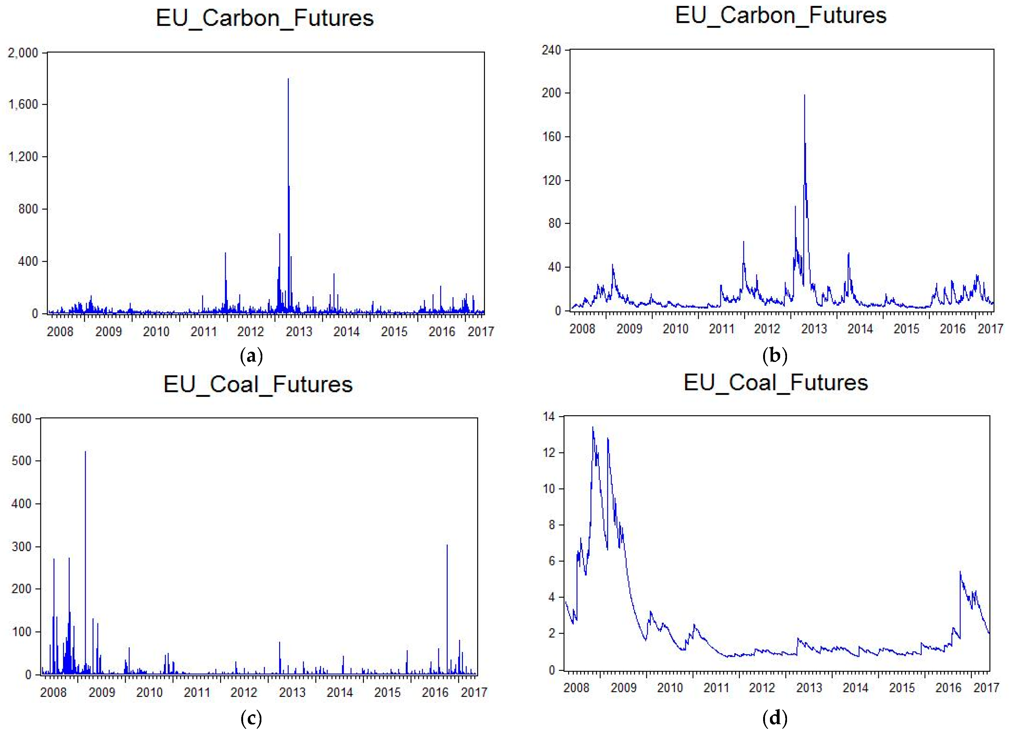
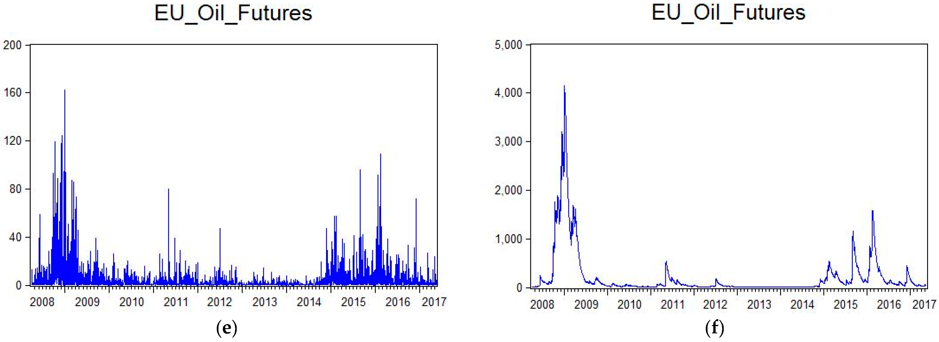
The unconditional and conditional volatility of carbon, coal, and oil futures returns for the EU are shown in Figure 4a–f, while the unconditional and conditional volatility of carbon, coal, and oil spot returns for the USA are shown in Figure 5a–f. The conditional volatility estimates are forecasts of the unconditional volatilities. Both figures show that there is a significant difference between the conditional and unconditional volatilities. As one of the purposes of the paper is to use conditional volatilities to forecast optimal hedge ratios for the various spot and futures returns, any differences between the unconditional and conditional volatilities is based on the unconditional volatilities being unpredictable as compared to the conditional volatilities.

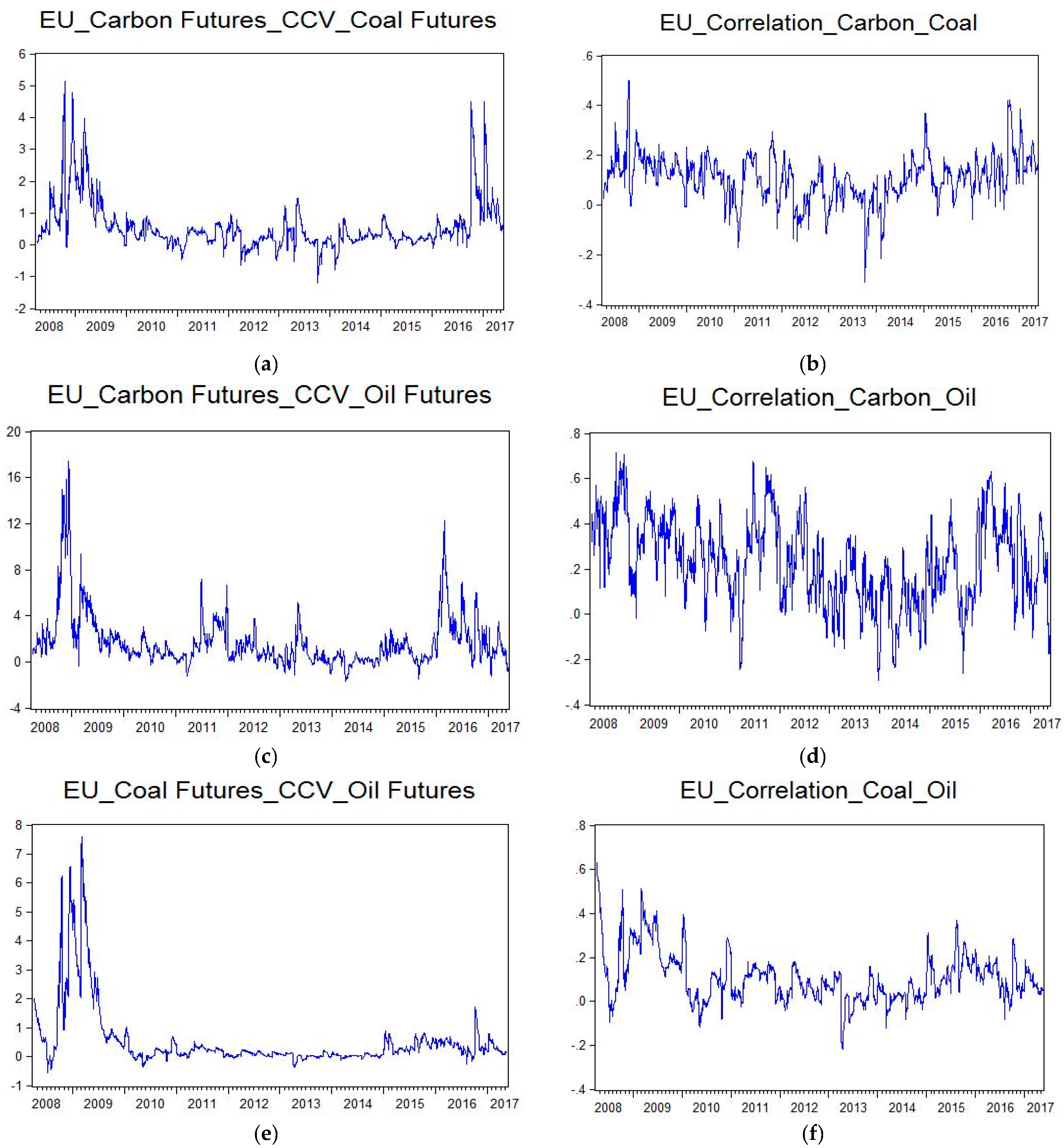
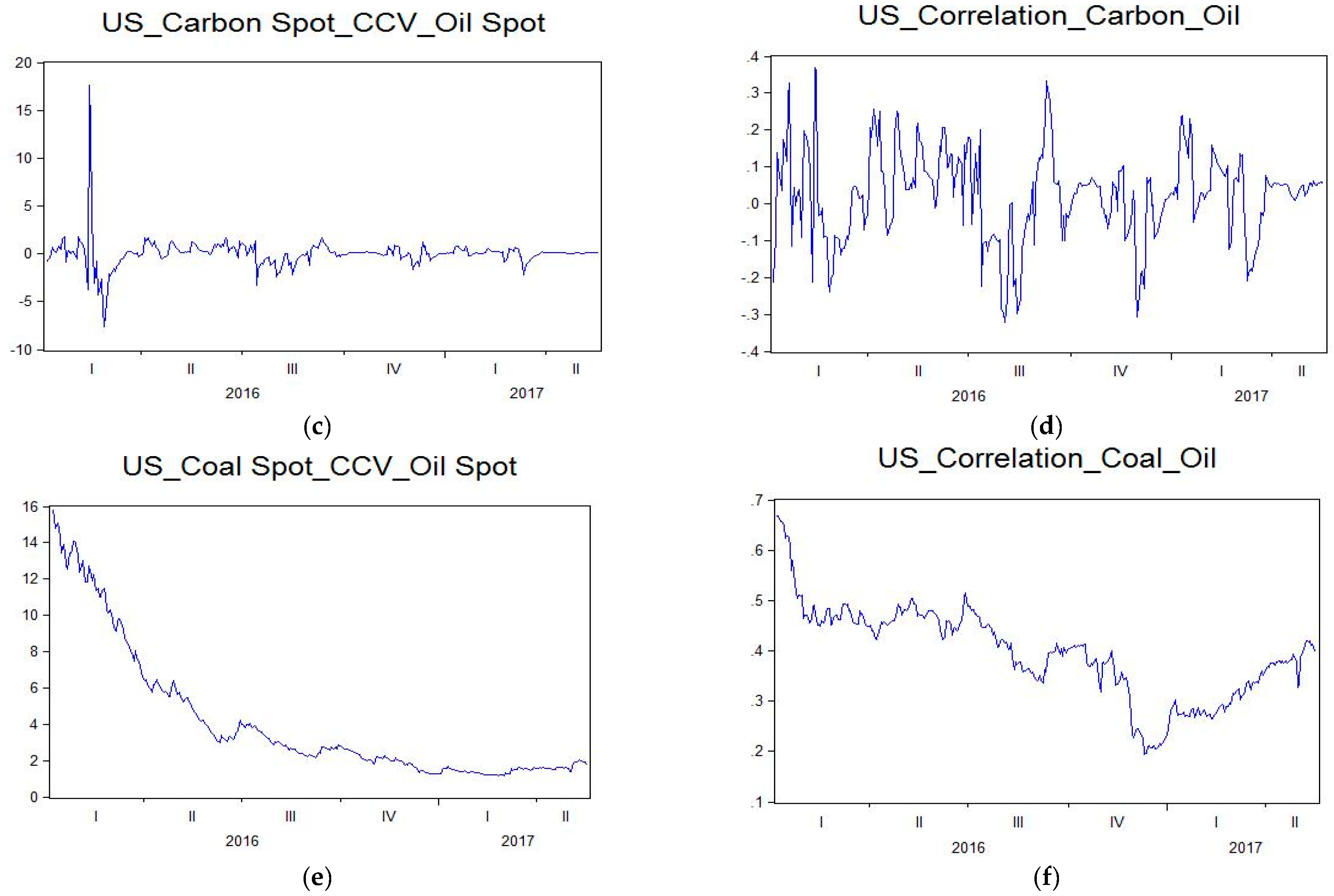
The conditional co-volatility correlations for carbon, coal, and oil futures returns for the EU are shown in Figure 6a–f, while the conditional co-volatility correlations for carbon, coal, and oil spot returns for the USA are shown in Figure 7a–f. Both of the figures show that there are substantial differences in the correlations of conditional co-volatility across the two markets and time periods for carbon, coal, and oil futures returns.

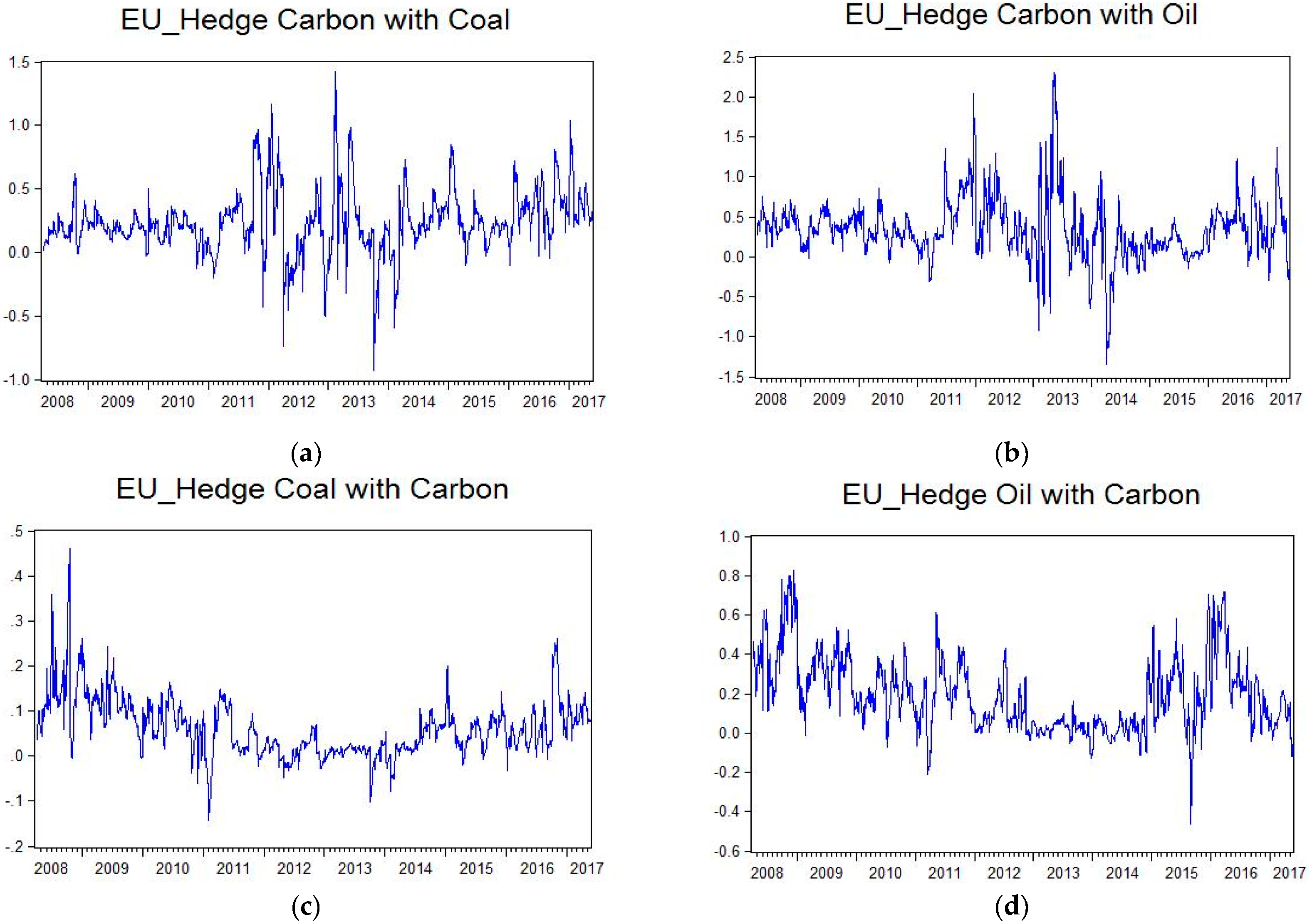
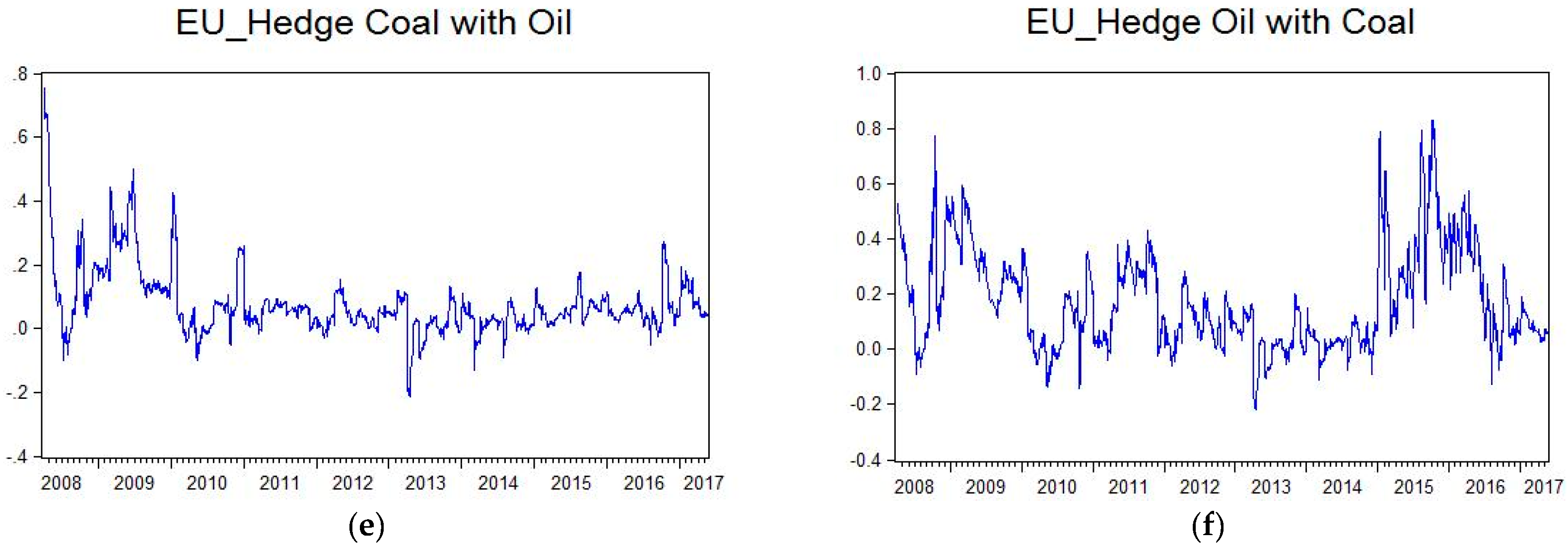
The optimal hedge ratios for carbon, coal, and oil futures returns for the EU, and optimal hedge ratios for carbon, coal, and oil spot returns for the USA, are given in Figure 8a–f and Figure 9a–f, respectively. The hedge ratios show how the covariances in returns between two assets changes relative to the variance of the hedging instrument. Both figures show that there is substantial variation in the optimal hedge ratios, so that the futures and spot prices of carbon emissions, coal, and oil should be considered contemporaneously and simultaneously in a portfolio that links the prices, returns, and volatilities of carbon emissions to the use of fossil fuels.

Finally, Figure 10a–d show the optimal hedge ratios for carbon futures returns for the EU and both coal and oil spot returns for the USA. In all cases, the optimal hedge ratios vary substantially, which suggests that it would be sensible to use both markets to hedge carbon emission futures returns in the EU against both coal and oil spot price returns in the USA.

6. Concluding Remarks

The paper discussed recent research that showed the efforts to limit climate change have been focusing on the reduction of carbon dioxide emissions over other greenhouse gases or air pollutants. Many countries have paid great attention to carbon emissions in order to improve air quality and public health. The largest source of carbon emissions from human activities in many countries in Europe and around the world has been from burning fossil fuels. The prices of both fuel and carbon emissions can and do have simultaneous and contemporaneous effects on each other.

Owing to the importance of carbon emissions and their interconnection to the prices, financial returns, and associated volatilities of fossil fuels, and the possibility of Granger causality in spot and futures prices, returns, and volatility of carbon emissions, it is not surprising that crude oil and coal, and their interactions with carbon emission prices, returns and volatility, have recently become very important for public policy and an associated research topic.

For the USA, daily spot and futures prices are available for crude oil and coal, but there are no daily spot or futures prices for carbon emissions. For the EU, there are no daily spot prices for coal or carbon emissions, but there are daily futures prices for crude oil, coal, and carbon emissions. For this reason, daily prices were used to analyse Granger causality and volatility spillovers in spot and futures prices of carbon emissions, crude oil, and coal.

A quasi likelihood ratio (QLR) test was developed to test the multivariate conditional volatility Diagonal BEKK model, which has valid regularity conditions and asymptotic properties, against the alternative Full BEKK model, which has valid regularity conditions and asymptotic properties only under the null hypothesis of zero off-diagonal elements. In short, Full BEKK has no desirable mathematical or statistical properties, except either under the null hypothesis of zero off-diagonal elements of the weighting matrix, or simply by assumption.

In the empirical analysis, DBEKK was rejected against the Full BEKK model for EU futures returns, but DBEKK was not rejected against Full BEKK for US spot returns. Therefore, further work would seem to be required for DBEKK in the case of EU futures returns, whereas DBEKK is empirically supported by the data for US spot returns.

Dynamic hedging strategies using optimal hedge ratios were suggested to analyse market fluctuations in the spot and futures returns and volatility of carbon emissions, crude oil, and coal prices. It was suggested that the futures and spot prices of carbon emissions, coal, and oil should be considered contemporaneously and simultaneously in a portfolio that links the prices, returns, and volatilities of carbon emissions to the use of fossil fuels. It would also be sensible to use the prices in both markets to hedge carbon emission price returns in the EU against both coal and oil spot price returns in the USA.

References

- Rogelj, J.; Meinshausen, M.; Sedláček, J.; Knutti, R. Implications of potentially lower climate sensitivity on climate projections and policy. Environ. Res. Lett. 2014, 9, 3–10. [Google Scholar] [CrossRef]
- Granger, C.W.J. Testing for causality: A personal viewpoint. J. Econ. Dyn. Control 1980, 2, 329–352. [Google Scholar] [CrossRef]
- Ramos, S.; Veiga, H. (Eds.) The Interrelationship between Financial and Energy Markets. In Lecture Notes in Energy; Springer: Berlin, Germany, 2014; Volume 54. [Google Scholar]
- Sawik, B.; Faulin, J.; Pérez-Bernabeu, E. A multicriteria analysis for the green VRP: A case discussion for the distribution problem of a Spanish retailer. Transp. Res. Proced. 2017, 22, 305–313. [Google Scholar] [CrossRef]
- Sawik, B.; Faulin, J.; Pérez-Bernabeu, E. Multi-objective traveling salesman and transportation problem with environmental aspects. In Applications of Management Science; Lawrence, K.D., Kleinman, G., Eds.; Emerald: Bingley, UK, 2017; Volume 18, pp. 21–56. [Google Scholar]
- Sawik, B.; Faulin, J.; Pérez-Bernabeu, E. Selected multi-criteria green vehicle routing problems. In Applications of Management Science; Lawrence, K.D., Kleinman, G., Eds.; Emerald: Bingley, UK, 2017; Volume 18, pp. 57–84. [Google Scholar]
- Hafner, C.M.; Herwartz, H. A Lagrange multiplier test for causality in variance. Econ. Lett. 2006, 93, 137–141. [Google Scholar] [CrossRef]
- Chang, C.-L.; McAleer, M. A simple test for causality in volatility. Econometrics 2017, 5, 15. [Google Scholar] [CrossRef]
- Baba, Y.; Engle, R.F.; Kraft, D.; Kroner, K.F. Multivariate Simultaneous Generalized ARCH; Unpublished manuscript; Department of Economics, University of California: San Diego, CA, USA, 1985. [Google Scholar]
- Engle, R.F.; Kroner, K.F. Multivariate simultaneous generalized ARCH. Econom. Theory 1995, 11, 122–150. [Google Scholar] [CrossRef]
- Bollerslev, T. Modelling the coherence in short-run nominal exchange rate: A multivariate generalized ARCH approach. Rev. Econ. Stat. 1990, 72, 498–505. [Google Scholar] [CrossRef]
- Ling, S.; McAleer, M. Asymptotic theory for a vector ARMA-GARCH model. Econom. Theory 2003, 19, 280–310. [Google Scholar] [CrossRef]
- McAleer, M.S.; Hoti, F. Chan Structure and asymptotic theory for multivariate asymmetric conditional volatility. Econom. Rev. 2009, 28, 422–440. [Google Scholar] [CrossRef]
- McAleer, M.F.; Chan, S.; Hoti, O. Lieberman Generalized autoregressive conditional correlation. Econom. Theory 2008, 24, 1554–1583. [Google Scholar] [CrossRef]
- Chang, C.-L.; McAleer, M. The Fiction of Full BEKK; Tinbergen Institute Discussion Paper 17–015; Tinbergen Institute: Amsterdam, The Netherlands, 2017. [Google Scholar]
- Hafner, C.; McAleer, M. A One Line Derivation of DCC: Application of a Vector Random Coefficient Moving Average Process; Tinbergen Institute Discussion Paper 14–087; Tinbergen Institute: Amsterdam, The Netherland, 2014. [Google Scholar]
- McAleer, M. Stationarity and Invertibility of a Dynamic Correlation Matrix; Tinbergen Institute Discussion Paper 17–082; Tinbergen Institute: Amsterdam, The Netherland, 2017. [Google Scholar]
- Caporin, M.; McAleer, M. Do we really need both BEKK and DCC? A tale of two multivariate GARCH models. J. Econ. Surv. 2012, 26, 736–751. [Google Scholar] [CrossRef]
- Chang, C.-L.; Li, Y.-Y.; McAleer, M. Volatility Spillovers between Energy and Agricultural Markets: A Critical Appraisal of Theory and Practice; Tinbergen Institute Discussion Paper 15–077/III; Tinbergen Institute: Amsterdam, The Netherland, 2015. [Google Scholar]
- Chang, C.-L.; McAleer, M.; Wang, Y.-A. Modelling volatility spillovers for bio-ethanol, sugarcane and corn spot and futures prices. Renew. Sustain. Energy Rev. 2017, 81, 1002–1018. [Google Scholar] [CrossRef]
- Tsay, R.S. Conditional heteroscedastic time series models. J. Am. Stat. Assoc. 1987, 82, 590–604. [Google Scholar] [CrossRef]
- Engle, R.F. Autoregressive conditional heteroskedasticity with estimates of the variance of United Kingdom inflation. Econometrica 1982, 50, 987–1007. [Google Scholar] [CrossRef]
- Bollerslev, T. Generalized autoregressive conditional heteroscedasticity. J. Econom. 1986, 31, 307–327. [Google Scholar] [CrossRef]
- Jeantheau, T. Strong consistency of estimators for multivariate ARCH models. Econom. Theory 1998, 14, 70–86. [Google Scholar] [CrossRef]
- Amemiya, T. Advanced Econometrics; Harvard University Press: Cambridge, MA, USA, 1985. [Google Scholar]
- Asai, M.; Chang, C.-L.; McAleer, M. Realized stochastic volatility with general asymmetry and long memory. J. Econom. 2017, 199, 202–212. [Google Scholar] [CrossRef]
- Dickey, D.A.; Fuller, W.A. Distribution of the estimators for autoregressive time series with a unit root. J. Am. Stat. Assoc. 1979, 74, 427–431. [Google Scholar]
- Dickey, D.A.; Fuller, W.A. Likelihood ratio statistics for autoregressive time series with a unit root. Econometrica 1981, 49, 1057–1072. [Google Scholar] [CrossRef]
- Said, S.E.; Dickey, D.A. Testing for unit roots in autoregressive-moving average models of unknown order. Biometrika 1984, 71, 599–607. [Google Scholar] [CrossRef]
- Elliott, G.; Rothenberg, T.J.; Stock, J.H. Efficient tests for an autoregressive unit root. Econometrica 1996, 64, 813–836. [Google Scholar] [CrossRef]
- Kwiatkowski, D.; Phillips, P.C.B.; Schmidt, P.; Shin, Y. Testing the null hypothesis of stationarity against the alternative of a unit root: How sure are we that economic time series have a unit root? J. Econom. 1992, 54, 159–178. [Google Scholar] [CrossRef]
Figure 1.
Global mean temperatures. With and without carbon dioxide mitigation. Source: [1] Rogelj et al. (2014).
Figure 2.
Implementation of programs to mitigate carbon emissions.
Figure 3.
Carbon futures and spot volumes for European Union (EU) 10 December 2012–19 May 2017.
Figure 4.
Unconditional (a,c,e) and Conditional (b,d,f) Volatility of Carbon, Coal, and Oil Futures for EU 2 April 2008–19 May 2017.
Figure 5.
Unconditional (a,c,e) and Conditional (b,d,f) Volatility of Carbon, Coal, Oil Spot for USA 6 January 2016–19 May 2017.
Figure 6.
Conditional Co-volatility (a,c,e) and Correlations (b,d,f) for Carbon, Coal, and Oil Futures for EU 2 April 2008–18 May 2017.
Figure 7.
Conditional Co-volatility (a,c,e) and Correlations (b,d,f) for Carbon, Coal, Oil Spot for USA 6 January 2016–18 May 2017.
Figure 8.
Optimal Hedge Ratios for Carbon (a,b), Coal (c,e), and Oil (d,f) Futures for EU 2 April 2008–19 May 2017.
Figure 9.
Optimal Hedge Ratios for Carbon (a,b), Coal (c,e), and Oil (d,f) Spot for USA 6 January 2016–18 May 2017.
Figure 10.
Optimal Hedge Ratios for Carbon (a,b) Futures of EU, and Coal (c) and Oil (d) Spot of USA 2 April 2008–18 May 2017.