

Multi-Model Rice Canopy Chlorophyll Content Inversion Based on UAV Hyperspectral Images

Abstract
:1. Introduction
2. Materials and Methods
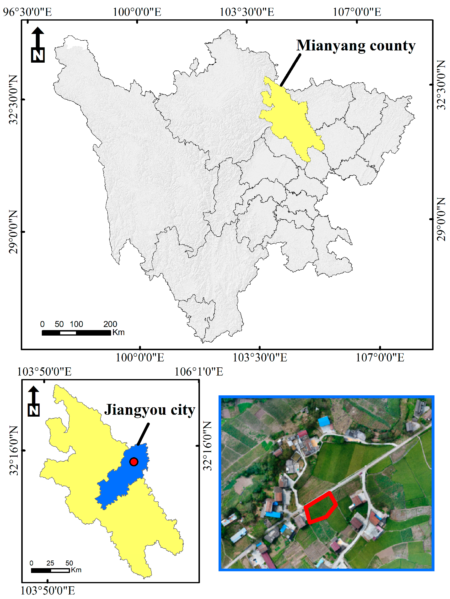
2.1. Overview of the Study Area
2.2. Composition of Remote Sensing System
2.3. Image and Data Acquisition
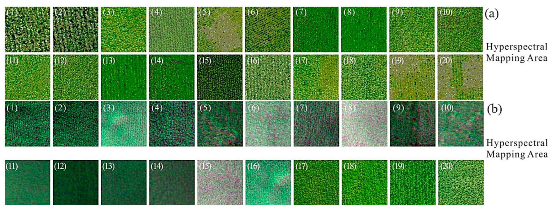
2.3.1. Hyperspectral Image Acquisition
2.3.2. Determination of SPAD Values of Rice Canopy in the Field
2.3.3. Hyperspectral Image Processing
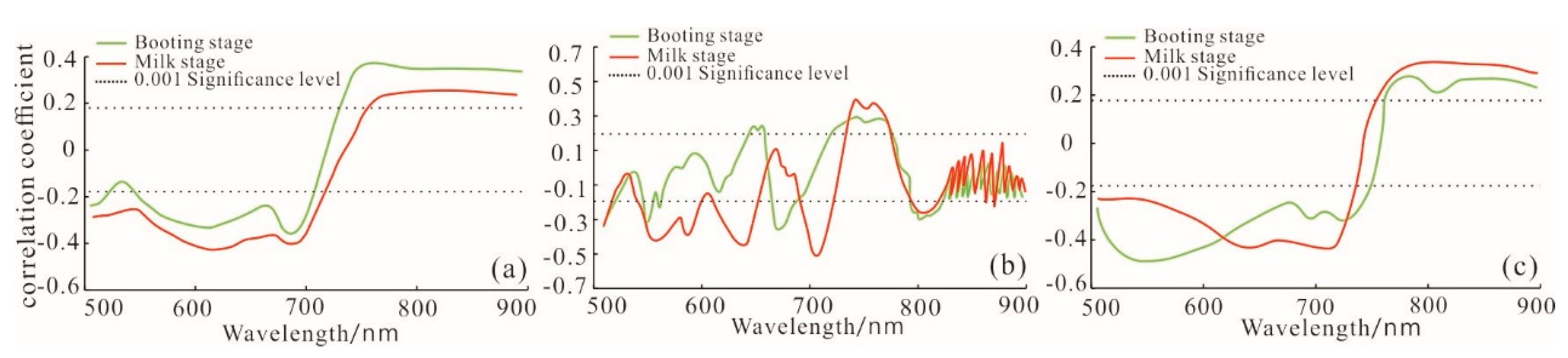
2.3.4. Spectral Feature Analysis and Extraction of Sensitive Bands
2.4. Methods
2.4.1. Univariate Regression
2.4.2. Partial Least Squares Regression (PLSR)
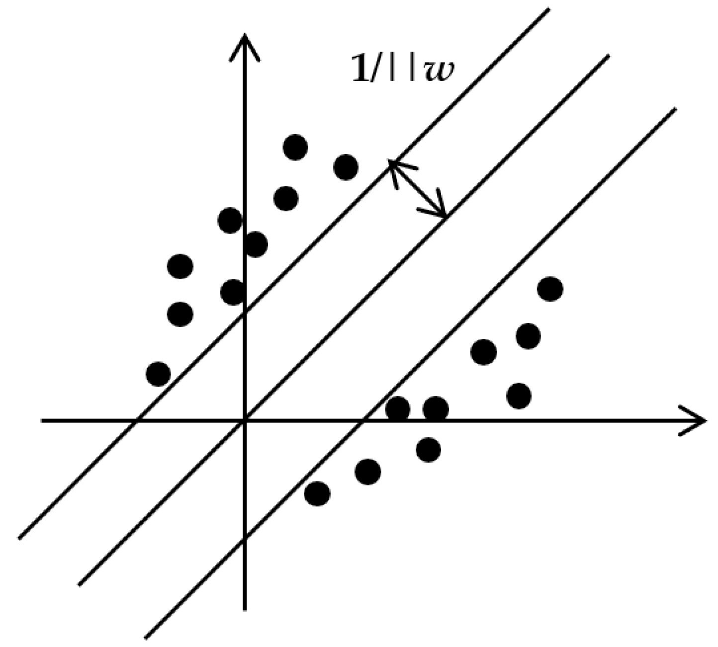
2.4.3. Support Vector Machine Regression (SVR)
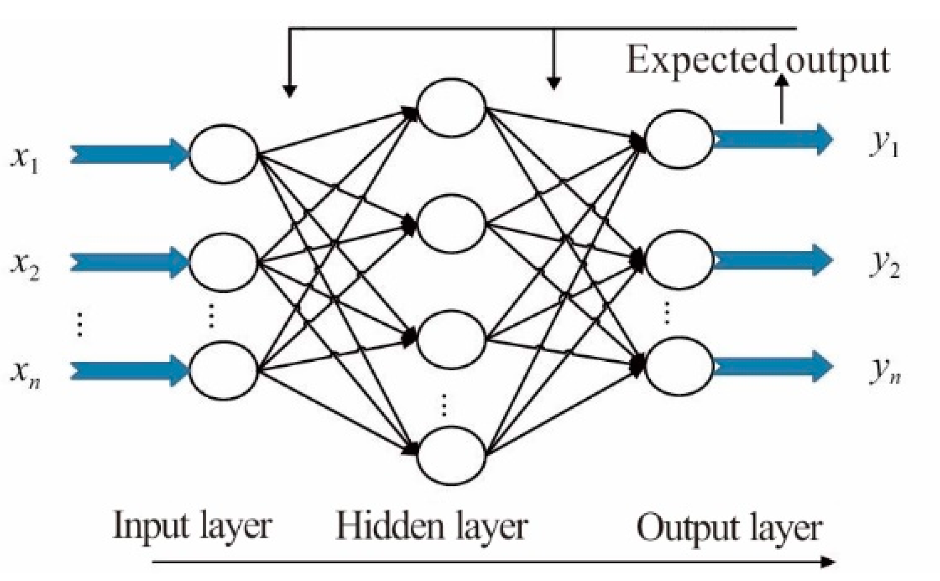
2.4.4. The BP Neural Network Regression
3. Results and Discussion
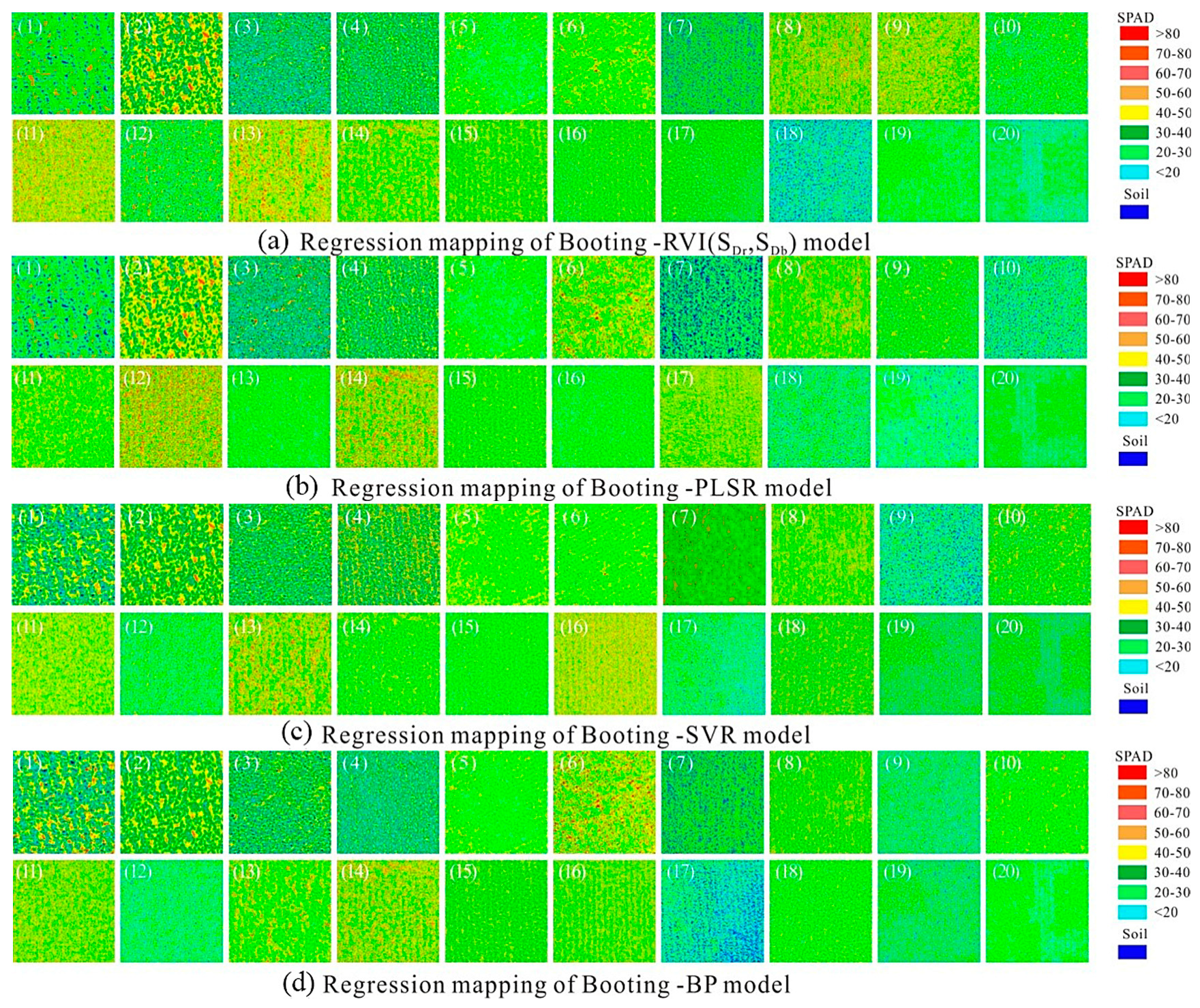
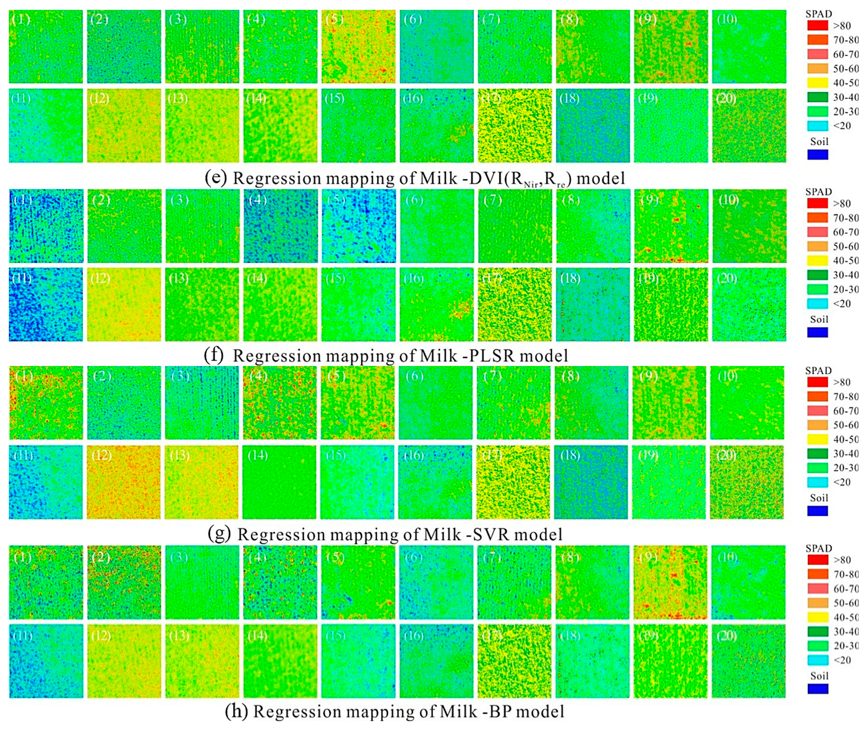
3.1. Model Construction
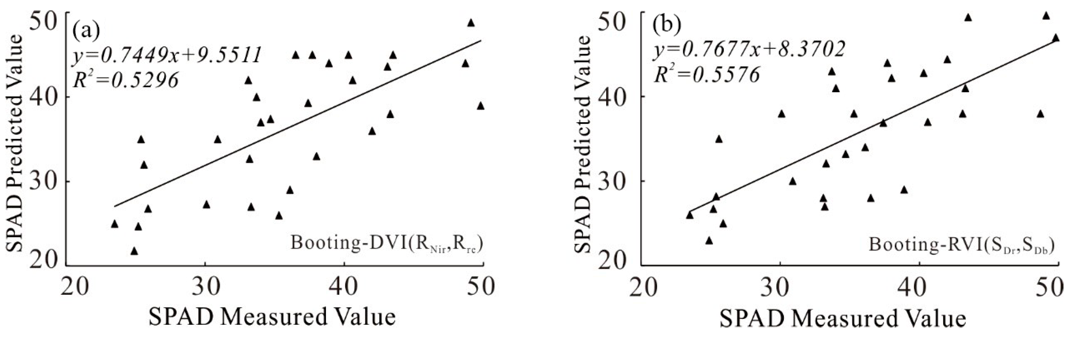
3.1.1. Model Construction Based on Univariate Regression
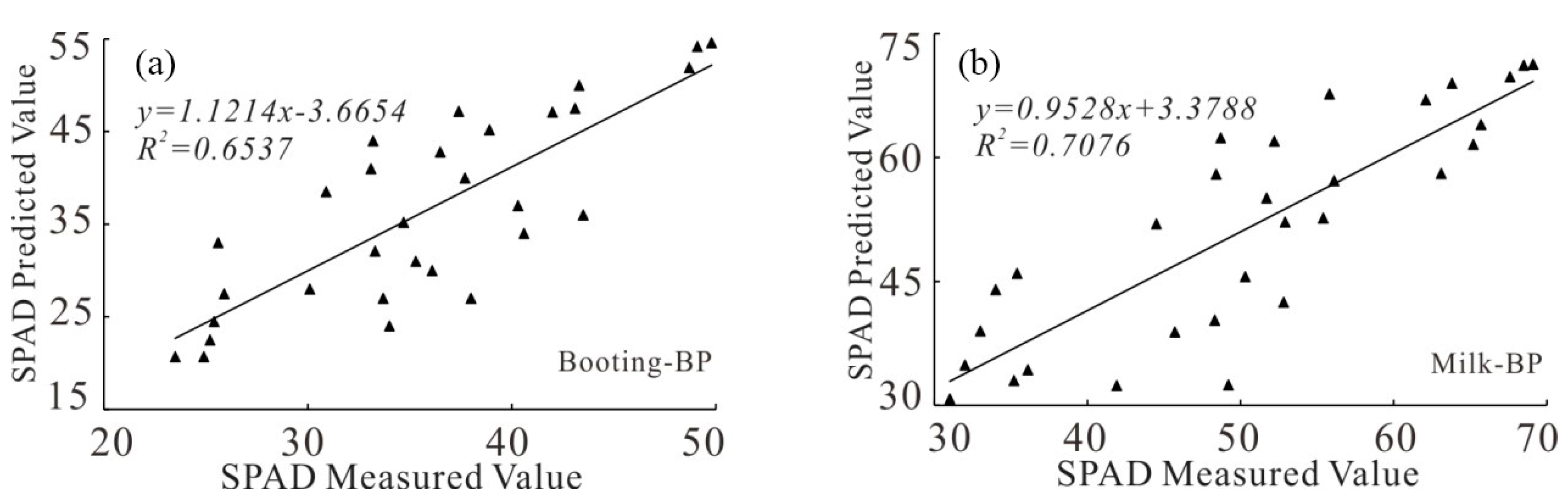
3.1.2. Model Construction Based on Partial Least Squares Regression (PLSR)
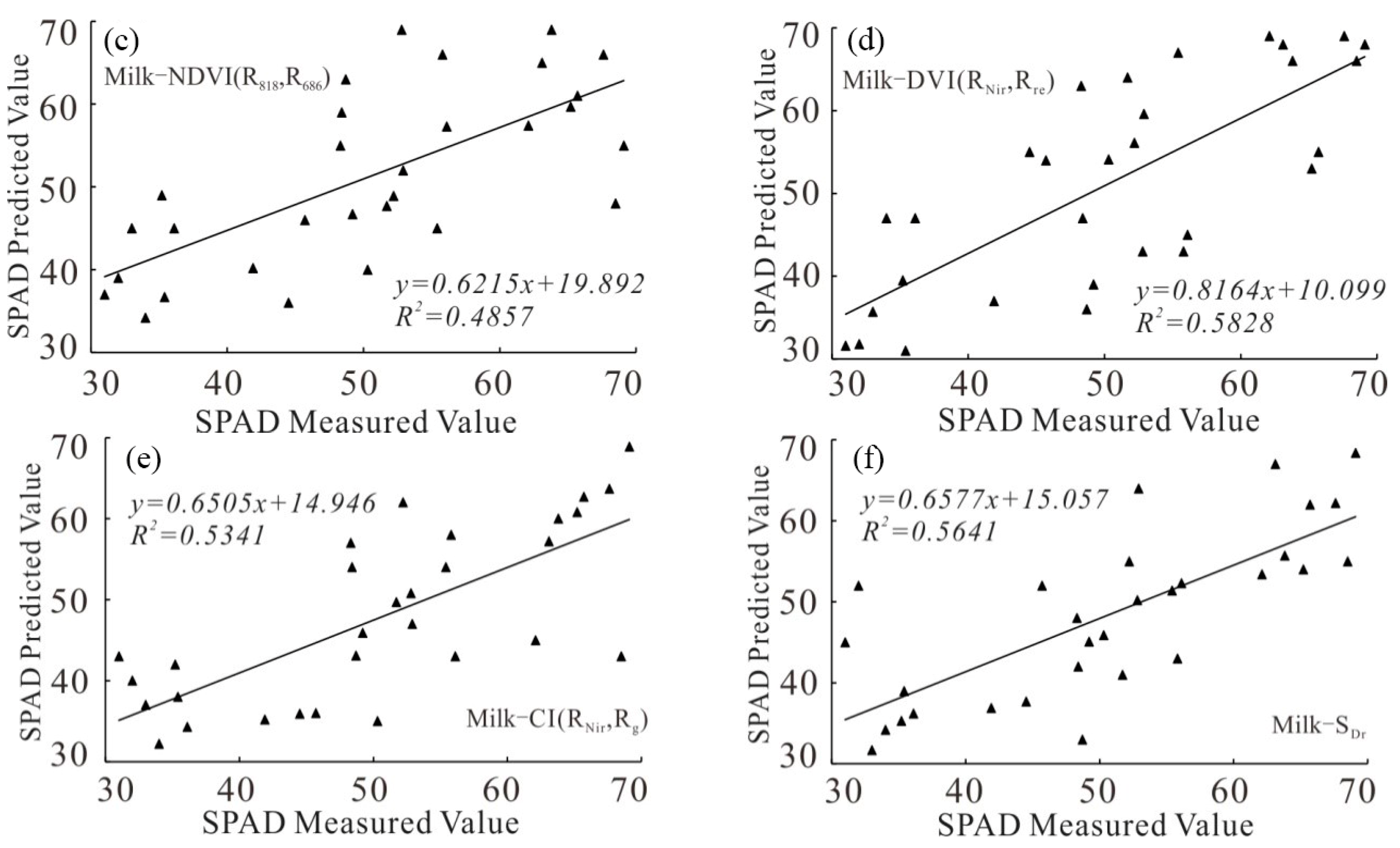
3.1.3. Model Construction Based on Support Vector Machine Regression (SVR)
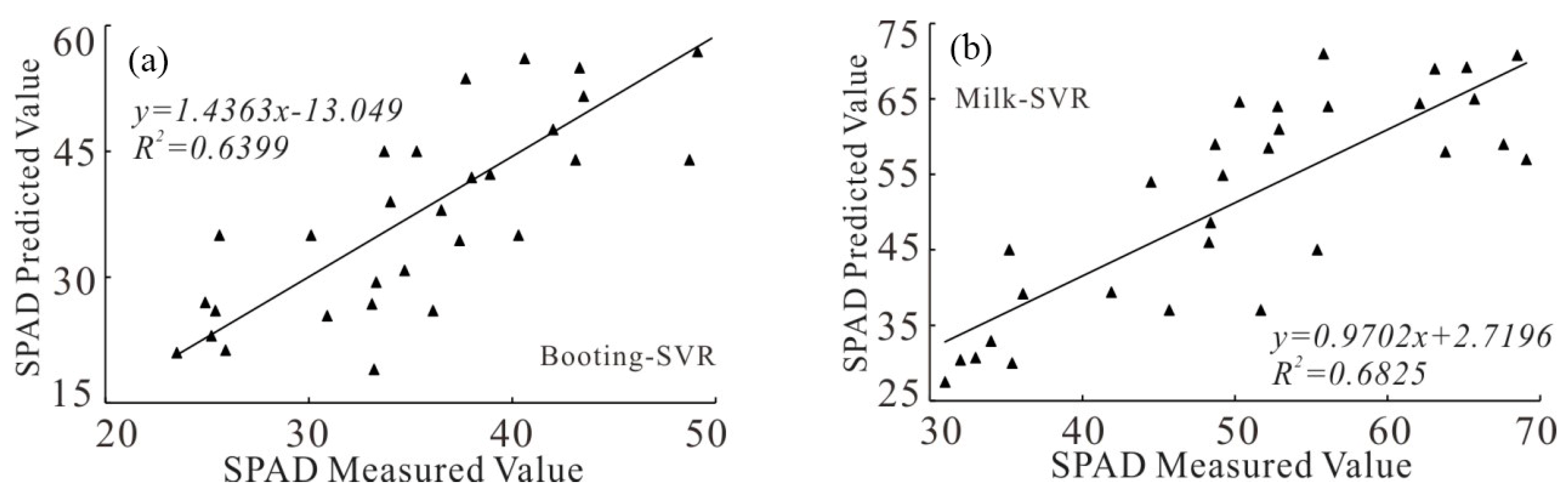
3.1.4. Model Construction Based on BP Neural Network Regression
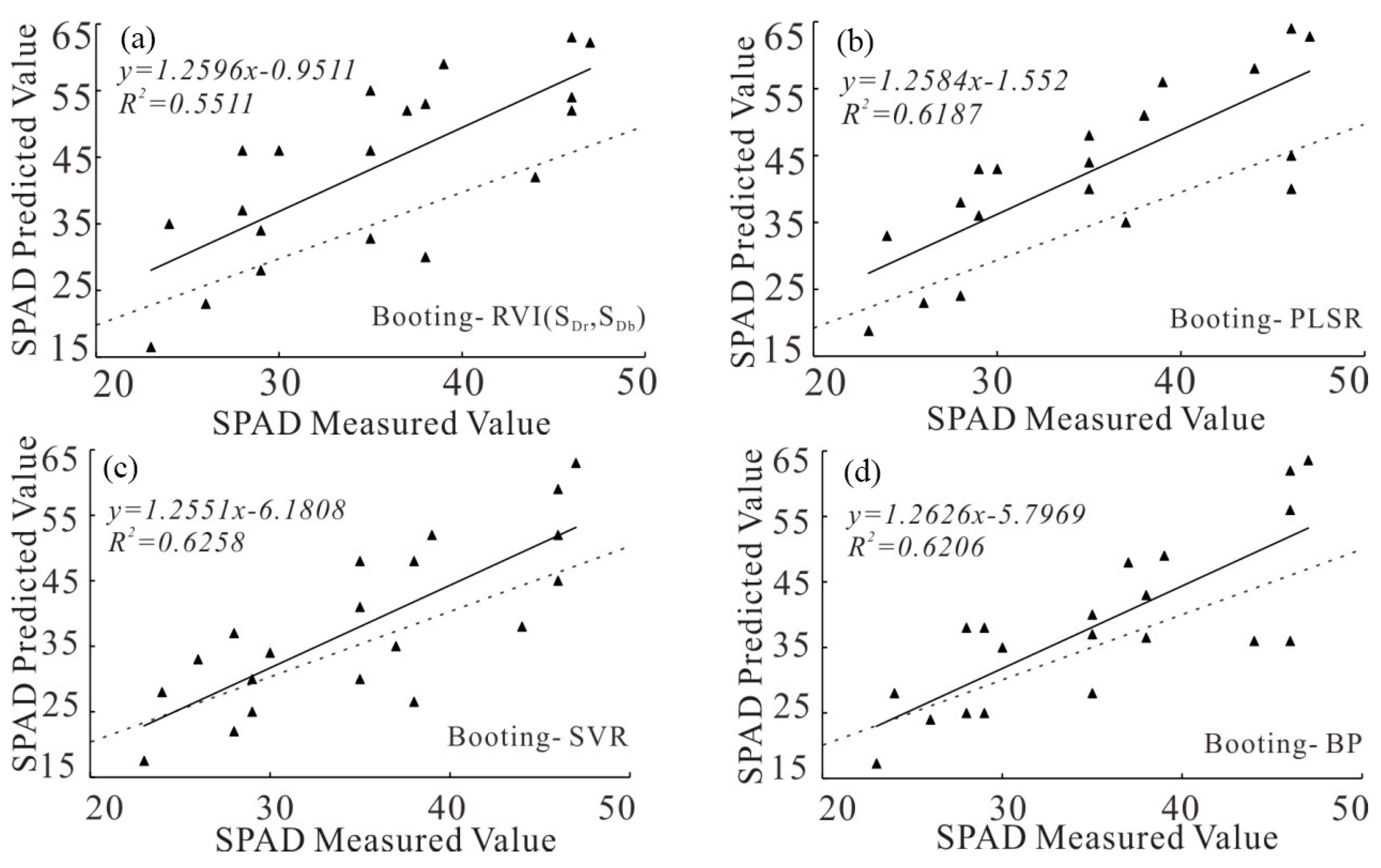
3.2. Model Accuracy Analysis
3.2.1. Univariate Model Accuracy Analysis
3.2.2. PLSR Model Accuracy Analysis
3.2.3. SVR Model Accuracy Analysis
3.2.4. BP Neural Network Model Accuracy Analysis
3.3. Optimal Inversion Model Selection
4. Conclusions
Author Contributions
Funding
Institutional Review Board Statement
Informed Consent Statement
Data Availability Statement
Acknowledgments
Conflicts of Interest
References
- Hu, T.; Chen, Y.; Li, D.; Long, C.; Wen, Z.; Hu, R.; Chen, G. Rice Variety Identification Based on the Leaf Hyperspectral Feature via LPP-SVM. Int. J. Pattern Recognit. Artif. Intell. 2022, 36, 17. [Google Scholar] [CrossRef]
- Luo, Y.; Huang, D.; Li, D.; Wu, L. On farm storage, storage losses and the effects of loss reduction in China. Resour. Conserv. Recycl. 2020, 162, 9. [Google Scholar] [CrossRef]
- Xiao, X.M.; Boles, S.; Liu, J.Y. Mapping paddy rice agriculture in southern China using multi-temporal MODIS images. Remote Sens. Environ. 2005, 95, 480–492. [Google Scholar] [CrossRef]
- Xu, Y.B.; Li, J.Y.; Wan, J.M. Agriculture and crop science in China: Innovation and sustainability. Crop J. 2017, 5, 95–99. [Google Scholar] [CrossRef]
- Chen, T.; Fu, W.; Yu, J.; Feng, B.; Li, G.; Fu, G.; Tao, L. The Photosynthesis Characteristics of Colored Rice Leaves and Its Relation with Antioxidant Capacity andAnthocyanin Content. Sci. Agric. Sin. 2022, 55, 12. [Google Scholar]
- Li, X.; Lu, X.; Xi, J.; Zhang, Y.; Zhang, M. Univeisal method to detect the chlorophyll content in plant leaves with RGB images captured by smart phones. Trans. Chin. Soc. Agric. Eng. 2021, 37, 7. [Google Scholar]
- Ravier, C.; Quemada, M.; Jeuffroy, M.-H. Use of a chlorophyll meter to assess nitrogen nutrition index during the growth cycle in winter wheat. Field Crops Res. 2017, 214, 73–82. [Google Scholar] [CrossRef]
- Ganeva, D.; Roumenina, E.; Dimitrov, P. Phenotypic Traits Estimation and Preliminary Yield Assessment in Different Phenophases of Wheat Breeding Experiment Based on UAV Multispectral Images. Remote Sens. 2022, 14, 1019. [Google Scholar] [CrossRef]
- Filion, R.; Bernier, M.; Paniconi, C. Remote sensing for mapping soil moisture and drainage potential in semi-arid regions: Applications to the Campidano plain of Sardinia, Italy. Sci. Total Environ. 2016, 543, 862–876. [Google Scholar] [CrossRef]
- Mulla, D.J. Twenty five years of remote sensing in precision agriculture: Key advances and remaining knowledge gaps. Biosyst. Eng. 2013, 114, 358–371. [Google Scholar] [CrossRef]
- Weiss, M.; Jacob, F.; Duveiller, G. Remote sensing for agricultural applications: A meta-review. Remote Sens. Environ. 2020, 236, 111402. [Google Scholar] [CrossRef]
- Tao, H.; Feng, H.; Xu, L.; Miao, M.; Long, H.; Yue, J.; Li, Z.; Yang, G.; Yang, X.; Fan, L. Estimation of Crop Growth Parameters Using UAV-Based Hyperspectral Remote Sensing Data. Sensors 2020, 20, 1296. [Google Scholar] [CrossRef] [PubMed]
- Burkart, A.; Cogliati, S.; Schickling, A.; Rascher, U. A Novel UAV-Based Ultra-Light Weight Spectrometer for Field Spectroscopy. IEEE Sens. J. 2014, 14, 62–67. [Google Scholar] [CrossRef]
- Wei, Z.; Han, Y.; Li, M.; Yang, K.; Yang, Y.; Luo, Y.; Ong, S.-H. A Small UAV Based Multi-Temporal Image Registration for Dynamic Agricultural Terrace Monitoring. Remote Sens. 2017, 9, 904. [Google Scholar] [CrossRef]
- Huang, Y.; Ma, Q.; Wu, X.; Li, H.; Xu, K.; Ji, G.; Qian, F.; Li, L.; Huang, Q.; Long, Y.; et al. Estimation of chlorophyll content in Brassica napus based on unmanned aerial vehicle images. Oil Crop Sci. 2022, 7, 149–155. [Google Scholar] [CrossRef]
- Kim, E.-J.; Nam, S.-H.; Koo, J.-W.; Hwang, T.-M. Hybrid Approach of Unmanned Aerial Vehicle and Unmanned Surface Vehicle for Assessment of Chlorophyll-a Imagery Using Spectral Indices in Stream, South Korea. Water 2021, 13, 1930. [Google Scholar] [CrossRef]
- Ballesteros, R.; Ortega, J.F.; Hernández, D.; Moreno, M.A. Applications of georeferenced high-resolution images obtained with unmanned aerial vehicles. Part II: Application to maize and onion crops of a semi-arid region in Spain. Precis. Agric. 2014, 15, 593–614. [Google Scholar] [CrossRef]
- Calderón, R.; Navas-Cortés, J.A.; Lucena, C.; Zarco-Tejada, P.J. High-resolution airborne hyperspectral and thermal imagery for early, detection of Verticillium wilt of olive using fluorescence, temperature and narrow-band spectral indices. Remote Sens. Environ. 2013, 139, 231–245. [Google Scholar] [CrossRef]
- Panigrahi, N.; Das, B.S. Canopy Spectral Reflectance as a Predictor of Soil Water Potential in Rice. Water Resour. Res. 2018, 54, 2544–2560. [Google Scholar] [CrossRef]
- Poblete-Echeverría, C.; Olmedo, G.F.; Ingram, B.; Bardeen, M. Detection and Segmentation of Vine Canopy in Ultra-High Spatial Resolution RGB Imagery Obtained from Unmanned Aerial Vehicle (UAV): A Case Study in a Commercial Vineyard. Remote Sens. 2017, 9, 268. [Google Scholar] [CrossRef]
- Gitelson, A.A.; Peng, Y.; Arkebauer, T.J. Relationships between gross primary production, green LAI, and canopy chlorophyll content in maize: Implications for remote sensing of primary production. Remote Sens. Environ. 2014, 144, 65–72. [Google Scholar] [CrossRef]
- He, Z.; Wu, K.; Wang, F.; Jin, L.; Zhang, R.; Tian, S.; Wu, W.; He, Y.; Huang, R.; Yuan, L.; et al. Fresh Yield Estimation of Spring Tea via Spectral Differences in UAV Hyperspectral Images from Unpicked and Picked Canopies. Remote. Sens. 2023, 15, 1100. [Google Scholar] [CrossRef]
- Padalia, H.; Sinha, S.K.; Bhave, V.; Trivedi, N.K.; Kumar, A.S. Estimating canopy LAI and chlorophyll of tropical forest plantation (North India) using Sentinel-2 data. Adv. Space Res. 2020, 65, 458–469. [Google Scholar] [CrossRef]
- Thomas, V.; Treitz, P.; McCaughey, J.H.; Noland, T.; Rich, L. Canopy chlorophyll concentration estimation using hyperspectral and lidar data for a boreal mixedwood forest in northern Ontario, Canada. Int. J. Remote Sens. 2008, 29, 1029–1052. [Google Scholar] [CrossRef]
- Feng, M.C.; Guo, X.L.; Wang, C. Monitoring and evaluation in freeze stress of winter wheat (Triticum aestivum L.) through canopy hyperspectrum reflectance and multiple statistical analysis. Ecol. Indic. 2018, 84, 290–297. [Google Scholar] [CrossRef]
- Shi, H.; Guo, J.; An, J.; Tang, Z.; Wang, X.; Li, W.; Zhao, X.; Jin, L.; Xiang, Y.; Li, Z.; et al. Estimation of Chlorophyll Content in Soybean Crop at Different Growth Stages Based on Optimal Spectral Index. Agronomy 2023, 13, 663. [Google Scholar] [CrossRef]
- Liang, L.; Qin, Z.; Zhao, S.; Di, L.; Zhang, C.; Deng, M.; Lin, H.; Zhang, L.; Wang, L.; Liu, Z. Estimating crop chlorophyll content with hyperspectral vegetation indices and the hybrid inversion method. Int. J. Remote Sens. 2016, 37, 2923–2949. [Google Scholar] [CrossRef]
- Milas, A.S.; Romanko, M.; Reil, P.; Abeysinghe, T.; Marambe, A. The importance of leaf area index in mapping chlorophyll content of corn under different agricultural treatments using UAV images. Int. J. Remote Sens. 2018, 39, 5415–5431. [Google Scholar] [CrossRef]
- Wu, C.; Han, X.; Niu, Z.; Dong, J. An evaluation of EO-1 hyperspectral Hyperion data for chlorophyll content and leaf area index estimation. Int. J. Remote Sens. 2010, 31, 1079–1086. [Google Scholar] [CrossRef]
- Fageria, N.K. Yield physiology of rice. J. Plant Nutr. 2007, 30, 843–879. [Google Scholar] [CrossRef]
- Hlaváčová, M.; Klem, K.; Rapantová, B.; Novotná, K.; Urban, O.; Hlavinka, P.; Smutná, P.; Horáková, V.; Škarpa, P.; Pohanková, E.; et al. Interactive effects of high temperature and drought stress during stem elongation, anthesis and early grain filling on the yield formation and photosynthesis of winter wheat. Field Crops Res. 2018, 221, 182–195. [Google Scholar] [CrossRef]
- Guo, C.; Guo, X. Estimation of wetland plant leaf chlorophyll content based on continuum removal in the visible domain. Acta Ecol. Sin. 2016, 36, 6538–6546. [Google Scholar]
- Guo, Q.; Wu, X.; Bing, Q.; Pan, Y.; Wang, Z.; Fu, Y.; Wang, D.; Liu, J. Study on Retrieval of Chlorophyll-a Concentration Based on Landsat OLI Imagery in the Haihe River, China. Sustainability 2016, 8, 758. [Google Scholar] [CrossRef]
- Matus-Hernández, M.; Hernández-Saavedra, N.Y.; Martínez-Rincón, R.O. Predictive performance of regression models to estimate Chlorophyll-a concentration based on Landsat imagery. PLoS ONE 2018, 13, e0205682. [Google Scholar] [CrossRef]
- Ryan, K.; Ali, K. Application of a partial least-squares regression model to retrieve chlorophyll-aconcentrations in coastal waters using hyper-spectral data. Ocean Ence J. 2016, 51, 209–221. [Google Scholar]
- Song, K.; Lu, D.; Li, L.; Li, S.; Wang, Z.; Du, J. Remote sensing of chlorophyll-a concentration for drinking water source using genetic algorithms (GA)-partial least square (PLS) modeling. Ecol. Inform. 2012, 10, 25–36. [Google Scholar] [CrossRef]
- Kown, Y.; Baek, S.H.; Lim, Y.K.; Pyo, J.; Ligaray, M.; Park, Y.; Cho, K.H. Monitoring Coastal Chlorophyll-a Concentrations in Coastal Areas Using Machine Learning Models. Water 2018, 10, 1020. [Google Scholar] [CrossRef]
- Shao, Y.-H.; Chen, W.-J.; Deng, N.-Y. Nonparallel hyperplane support vector machine for binary classification problems. Inf. Sci. 2014, 263, 22–35. [Google Scholar] [CrossRef]
- Liu, M.; Liu, X.; Li, M.; Fang, M.; Chi, W. Neural-network model for estimating leaf chlorophyll concentration in rice under stress from heavy metals using four spectral indices. Biosyst. Eng. 2010, 106, 223–233. [Google Scholar] [CrossRef]
- Lu, F.; Chen, Z.; Liu, W.; Shao, H. Modeling chlorophyll-a concentrations using an artificial neural network for precisely eco-restoring lake basin. Ecol. Eng. 2016, 95, 422–429. [Google Scholar] [CrossRef]
- Buma, B. Evaluating the utility and seasonality of NDVI values for assessing post-disturbance recovery in a subalpine forest. Environ. Monit. Assess. 2012, 184, 3849–3860. [Google Scholar] [CrossRef] [PubMed]
- Gitelson, A.A.; Kaufman, Y.J.; Merzlyak, M.N. Use of a green channel in remote sensing of global vegetation from EOS-MODIS. Remote Sens. Environ. 1996, 58, 289–298. [Google Scholar] [CrossRef]
- Aasen, H.; Burkart, A.; Bolten, A. Generating 3D hyperspectral information with lightweight UAV snapshot cameras for vegetation monitoring: From camera calibration to quality assurance. ISPRS J. Photogramm. Remote Sens. 2015, 108, 245–259. [Google Scholar] [CrossRef]
- Haboudane, D.; Miller, J.R.; Tremblay, N.; Zarco-Tejada, P.J.; Dextraze, L. Integrated narrow-band vegetation indices for prediction of crop chlorophyll content for application to precision agriculture. Remote Sens. Environ. 2002, 81, 416–426. [Google Scholar] [CrossRef]
- Daughtry, C.S.T.; Walthall, C.L.; Kim, M.S. Estimating corn leaf chlorophyll concentration from leaf and canopy reflectance. Remote Sens. Environ. 2000, 74, 229–239. [Google Scholar] [CrossRef]
- Rodger, A.; Laukamp, C.; Haest, M.; Cudahy, T. A simple quadratic method of absorption feature wavelength estimation in continuum removed spectra. Remote Sens. Environ. 2012, 118, 273–283. [Google Scholar] [CrossRef]
- Dash, J.; Curran, P.J. Evaluation of the MERIS terrestrial chlorophyll index (MTCI). Adv. Space Res. 2007, 39, 100–104. [Google Scholar] [CrossRef]
- Cao, Q.; Miao, Y.X.; Shen, J.N. Improving in-season estimation of rice yield potential and responsiveness to topdressing nitrogen application with Crop Circle active crop canopy sensor. Precis. Agric. 2016, 17, 136–154. [Google Scholar] [CrossRef]
- Wang, F.-m.; Huang, J.-f.; Tang, Y.-l.; Wang, X.-z. New Vegetation Index and Its Application in Estimating Leaf Area Index of Rice. Rice Sci. 2007, 14, 195–203. [Google Scholar] [CrossRef]
- Gitelson, A.A.; Viña, A.; Ciganda, V.; Rundquist, D.C.; Arkebauer, T.J. Remote estimation of canopy chlorophyll content in crops. Geophys. Res. Lett. 2005, 32, L08403. [Google Scholar] [CrossRef]
- Kanke, Y.; Tubaña, B.; Dalen, M.; Harrell, D. Evaluation of red and red-edge reflectance-based vegetation indices for rice biomass and grain yield prediction models in paddy fields. Precis. Agric. 2016, 17, 507–530. [Google Scholar] [CrossRef]
- Ma, M.; Xu, T.; Zhou, Y. UAV HD Image Detection Method for SPAD in Northeast Japonica Rice. J. Shenyang Agric. Univ. 2017, 48, 757–762. [Google Scholar]
- Ban, S.; Liu, W.; Tian, M.; Wang, Q.; Yuan, T.; Chang, Q.; Li, L. Rice Leaf Chlorophyll Content Estimation Using UAV-Based Spectral Images in Different Regions. Agronomy 2022, 12, 2832. [Google Scholar] [CrossRef]
- Yuan, W.; Xu, T.; Cao, Y. Estimation of chlorophyll content in rice canopy leaves based on main base analysis and dimensionality reduction method. J. Zhejiang Univ. Agric. Life Sci. 2018, 44, 423–430. [Google Scholar]


| Growth Periods | Spectral Types | Sensitive Bands (nm) |
|---|---|---|
| Booting stage | Original spectrum | 567,686,770,818 |
| First derivative spectrum | 539,560,728,755 | |
| De-envelope spectrum | 525,686,735 | |
| milk-ripe stage | Original spectrum | 553,560,763 |
| First derivative spectrum | 518,546,728 | |
| De-envelope spectrum | 647,728,818 |
| Vegetation Index | Calculation Formulae or Definitions | Source of Formula |
|---|---|---|
| NDVI | (Rλi − Rλj)/(Rλi + Rλj) | [41] |
| DVI | RNir − Rre | [42] |
| SAVI | 1.5 (Rλi − Rλj)/(Rλi − Rλj + 0.5) | [43] |
| OSAVI | (1 + 0.16) (Rλi − Rλj)/(Rλi + Rλj + 0.16) | [43] |
| TCARI | 3[(Rλi − Rλj) − 0.2(Rλi − Rg)(Rλi/Rλj)] | [44] |
| MCARI | [(Rλi-Rλj) − 0.2(Rλi − Rg)](Rλi/Rλj) | [45] |
| RDVI | [46] | |
| MTCI | (Rλj − Rλi)/(Rλi − Rλk) | [47] |
| GRVI | Rλi/Rg | [48] |
| RNDVI | (Rλi − Rλj)/ | [49] |
| CI | RNir/Rg − 1 | [50] |
| RERDVI | (Rλi − Rre)/ | [51] |
| Characteristic Parameters | R2 | |
|---|---|---|
| Booting Stage | Milk-Ripe Stage | |
| NDVI (R818,R686) | 0.5216 | 0.6015 |
| DVI (RNir,Rre) | 0.6252 | 0.6126 |
| SAVI (R770,R647) | 0.5317 | 0.5791 |
| GRVI (R818,R518) | 0.5864 | 0.5215 |
| CI (RNir,Rg) | 0.5254 | 0.6136 |
| SDr | 0.5571 | 0.6042 |
| RVI (SDr,SDb) | 0.6158 | 0.5181 |
| Growth Stages | Parameters | Model Equations | R2 | RMSE |
|---|---|---|---|---|
| Booting stage | Feature parameters | y = −0.551x2 + 38.540x3 − 0.103x4 + 0.036x6 + 2.846x7 − 6.505 | 0.6341 | 9.9688 |
| Original spectrum | y = −0.515R567 + 1.445R686 + 0.585R770 + 1.017R818 − 44.006 | 0.6115 | 19.528 | |
| First derivative | y = 3.713R539 − 0.578R560 + 1.082R728 − 0.577R755 + 7.575 | 0.6150 | 16.0587 | |
| De-envelope | y = −0.455R525 + 1.650R686 + 1.709R735 − 24.809 | 0.6176 | 7.5396 | |
| Milk-ripe stage | Feature parameters | y = −32.968x1 − 1.716x2 − 4.567x3 + 6.608x4 + 0.925x5 − 0.501 | 0.6854 | 6.3586 |
| Original spectrum | y = 1.536R553 − 0.190R560 + 0.625R763 + 0.941 | 0.6181 | 22.5404 | |
| First derivative | y = 0.255R518 − 1.329R546 + 1.468R728 − 1.108 | 0.6029 | 5.0406 | |
| De-envelope | y = −0.551x2 + 38.540x3 − 0.103x4 + 0.036x6 + 2.846x7 − 6.505 | 0.6011 | 26.8097 |
| Growth Stages | Input Parameters | Kernel Function | C | |
|---|---|---|---|---|
| Booting stage | SAVI, GRVI, SDr | RBF | 100 | 0.1 |
| Milk-ripe stage | DVI, SAVI, CI, SDr | RBF | 100 | 0.1 |
| Hidden Layer Weights | 1 | 2 | 3 | 4 | 5 | 6 | 7 | 8 | |
|---|---|---|---|---|---|---|---|---|---|
| Input Layer Weights | |||||||||
| 1 | 0.2165 | 1.2019 | 1.2364 | −1.1247 | −1.1021 | 0.5656 | 0.3653 | 1.0321 | |
| 2 | −1.8763 | 0.3487 | 0.7825 | −0.9571 | −1.9274 | 1.1894 | 0.7453 | 0.7985 | |
| 3 | 1.0912 | −0.9875 | −0.6873 | 0.2094 | 1.3595 | −0.1209 | −1.2673 | 1.8632 | |
| 4 | 0.2317 | 0.5423 | −0.4501 | 1.7389 | 1.6120 | −0.1075 | 1.2984 | −0.5417 | |
| 5 | −0.7612 | 1.3211 | 1.2938 | −0.5210 | −1.9127 | −1.0836 | −0.1279 | −1.8237 | |
| Threshold (b) | 2.1835 | −1.5408 | 1.7225 | 0.7613 | 0.9187 | −0.6521 | 1.2013 | −1.6091 | |
| Hidden Layer Nodes | Weights | Threshold | Hidden Layer Nodes | Weights | Threshold |
|---|---|---|---|---|---|
| 1 | 1.9812 | 0.472 | 5 | −0.3017 | 0.472 |
| 2 | 0.4709 | 6 | 1.0145 | ||
| 3 | −1.3747 | 7 | 0.6430 | ||
| 4 | −0.5862 | 8 | −1.5436 |
| Hidden Layer Weights | 1 | 2 | 3 | 4 | 5 | 6 | 7 | 8 | |
|---|---|---|---|---|---|---|---|---|---|
| Input Layer Weights | |||||||||
| 1 | 1.1904 | −0.8730 | 0.5134 | −0.8107 | 1.3467 | 0.7564 | 1.3875 | −1.3108 | |
| 2 | 0.7237 | 1.5719 | −1.7891 | 1.3416 | 0.9134 | −1.1876 | 0.1283 | 1.0234 | |
| 3 | −1.5064 | 0.3781 | −0.3475 | −1.9871 | −0.3453 | −0.6034 | −0.8967 | 0.3246 | |
| 4 | 0.3984 | −1.0137 | −0.4501 | 0.3401 | 1.7486 | 1.8793 | −1.4113 | 1.2803 | |
| 5 | −1.1350 | 1.4503 | 1.2938 | −0.0519 | −0.5348 | −1.0434 | 0.1987 | −1.3146 | |
| Threshold (b) | 1.1701 | −1.1746 | −0.3114 | 0.3260 | −0.7408 | −1.8430 | −0.7634 | 0.8753 | |
| Hidden Layer Nodes | Weights | Threshold | Hidden Layer Nodes | Weights | Threshold |
|---|---|---|---|---|---|
| 1 | −1.4578 | 0.5015 | 5 | 1.3014 | 0.5015 |
| 2 | −0.3418 | 6 | 0.4357 | ||
| 3 | 2.0134 | 7 | −1.5834 | ||
| 4 | 1.3619 | 8 | 0.3101 |
| Models | Model Equations | R2 | RMSE | RE | |
|---|---|---|---|---|---|
| Booting stage | DVI(RNir,Rre) | y = 74.486x0.8695 | 0.5296 | 5.29 | 14.6 |
| RVI(SDr,SDb) | y = −0.0629x2 + 4.3705x + 9.9008 | 0.5576 | 5.15 | 14.3 | |
| Milk-ripe stage | NDVI(R818,R686) | y = 70.601x + 6.1291 | 0.4857 | 7.73 | 15.3 |
| DVI(RNir,Rre) | y = −10.817x2 + 101.17x + 17.075 | 0.5828 | 6.99 | 15.1 | |
| CI(RNir,Rg) | y = 0.1896x2 + 5.0079x + 25.901 | 0.5341 | 7.35 | 16.3 | |
| SDr | y = 0.0055x2 + 1.7285x − 13.78 | 0.5641 | 8.53 | 14.5 | |
| Growth Stages | Models | R2 | RMSE | RE |
|---|---|---|---|---|
| Booting stage | Booting stage-PLSR | 0.6228 | 7.17 | 21.2 |
| Milk-ripe stage | Milk-ripe stage-PLSR | 0.6757 | 9.12 | 17.9 |
| Growth Stages | Models | R2 | RMSE | RE |
|---|---|---|---|---|
| Booting stage | Booting stage-SVR | 0.6399 | 6.56 | 16.3 |
| Milk-ripe stage | Milk-ripe stage-SVR | 0.6825 | 8.11 | 14.7 |
| Growth Stages | Models | R2 | RMSE | RE |
|---|---|---|---|---|
| Booting stage | Booting stage-BP | 0.6537 | 5.68 | 15.2 |
| Milk-ripe stage | Milk-ripe stage-BP | 0.7076 | 8.22 | 17.6 |
| Growth Stages | Models | Gradient | R2 | RMSE | RE |
|---|---|---|---|---|---|
| Booting stage | RVI (SDr,SDb) | 1.2596 | 0.5511 | 9.1527 | 21.1 |
| PLSR | 1.2584 | 0.6187 | 7.9526 | 18.6 | |
| SVR | 1.2551 | 0.6258 | 7.8599 | 20.6 | |
| BP | 1.2626 | 0.6206 | 7.9001 | 20.6 | |
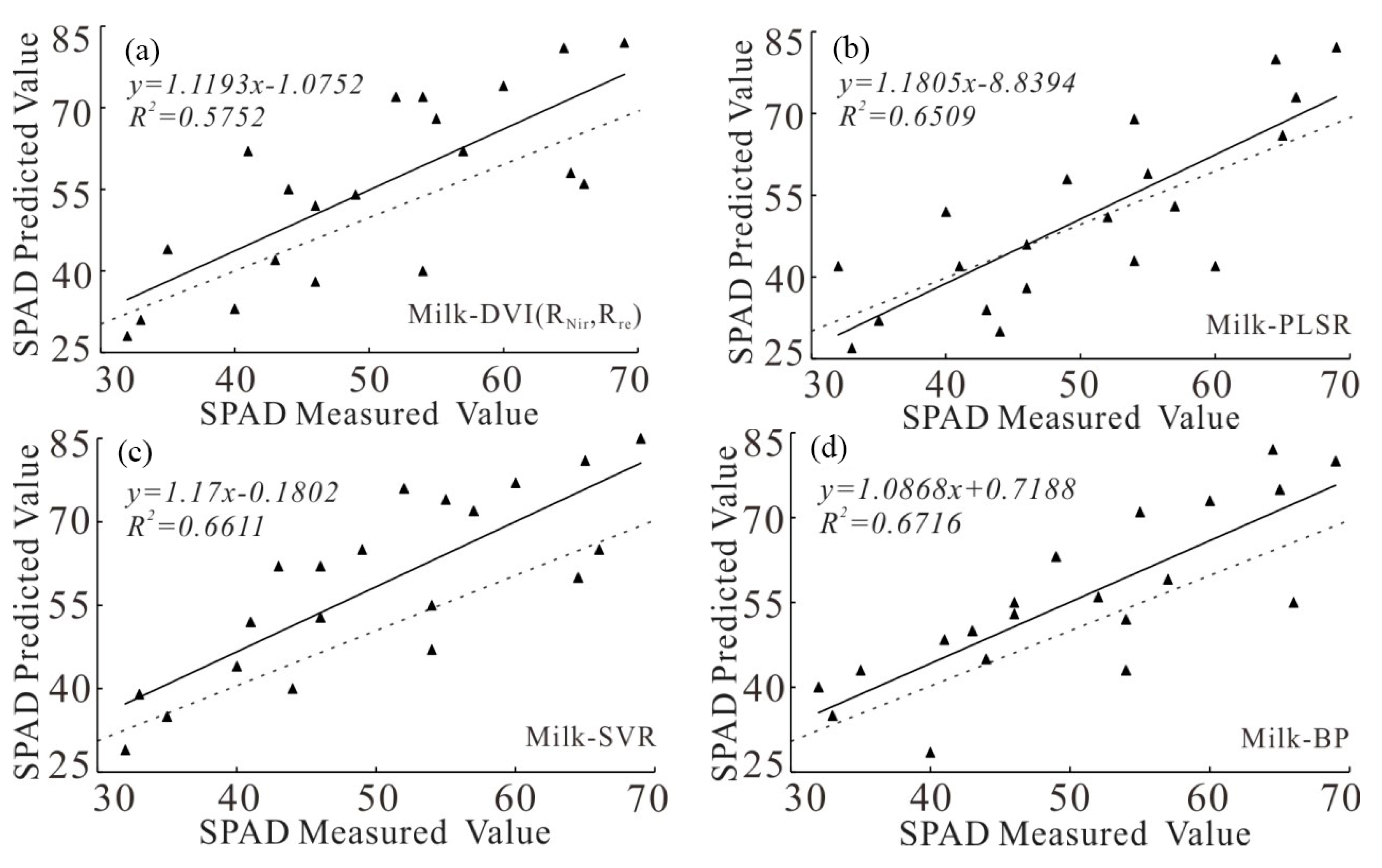
| Milk-ripe stage | DVI (RNir,Rre) | 1.1193 | 0.5752 | 11.1030 | 20.1 |
| PLSR | 1.1805 | 0.6509 | 9.9778 | 19.6 | |
| SVR | 1.17 | 0.6611 | 9.6688 | 16.5 | |
| BP | 1.0868 | 0.6716 | 8.7710 | 15.8 |
Disclaimer/Publisher’s Note: The statements, opinions and data contained in all publications are solely those of the individual author(s) and contributor(s) and not of MDPI and/or the editor(s). MDPI and/or the editor(s) disclaim responsibility for any injury to people or property resulting from any ideas, methods, instructions or products referred to in the content. |
© 2023 by the authors. Licensee MDPI, Basel, Switzerland. This article is an open access article distributed under the terms and conditions of the Creative Commons Attribution (CC BY) license (https://creativecommons.org/licenses/by/4.0/).
Share and Cite
Liu, H.; Lei, X.; Liang, H.; Wang, X. Multi-Model Rice Canopy Chlorophyll Content Inversion Based on UAV Hyperspectral Images. Sustainability 2023, 15, 7038. https://doi.org/10.3390/su15097038
Liu H, Lei X, Liang H, Wang X. Multi-Model Rice Canopy Chlorophyll Content Inversion Based on UAV Hyperspectral Images. Sustainability. 2023; 15(9):7038. https://doi.org/10.3390/su15097038
Chicago/Turabian StyleLiu, Hanhu, Xiangqi Lei, Hui Liang, and Xiao Wang. 2023. "Multi-Model Rice Canopy Chlorophyll Content Inversion Based on UAV Hyperspectral Images" Sustainability 15, no. 9: 7038. https://doi.org/10.3390/su15097038