Scanning Scheme for Underwater High-Rise Pile Cap Foundation Based on Imaging Sonar

Abstract

This study developed a sonar scanning scheme for underwater high-rise pile cap foundations (HRPCFs) to improve the efficiency of bridge inspection and prolong structural durability. First, two key factors in the measurement point arrangement that significantly affect the accuracy of sonar measurement—the appropriate range of measurement distance and the pitch angle—were determined experimentally. Subsequently, an assembled platform was designed to firmly hold the sonar and conveniently move it under strong currents to effectively provide clear images of the pile. A strategy was developed to determine the appropriate number and horizontal and vertical positions of the measurement points around each pile in the pile group, particularly to avoid the obstruction of signal propagation caused by adjacent piles and pile caps. The method was applied to the scanning of an underwater high-rise pile cap foundation of a bridge, and the results showed that the scanning ranges of the imaging sonar at all arranged measurement points were not affected by adjacent piles. The imaging sonar carried by the proposed platform could obtain clear images stably at a water speed of ~2.0 m/s and obtain all surface data of the pile quickly and completely.

1. Introduction

Recently, HRPCFs [1] have been widely used in the construction of sea-crossing bridges, wharves, and other off-shore infrastructures, and consist of a group of partially embedded piles and an elevated cap. However, the long-term impacts of water erosion, chloride ion erosion, and wet/dry cycles in the wave splash zone have caused the gradual degradation of the concrete protective layer surrounding bridge pile foundations, resulting in concrete spalling, cracks, and corrosion of the steel bars, which seriously affect the structural stability and safety of the bridge. Compared with the inspection of bridge superstructures, it is more challenging to inspect the bridge substructure defects because they are often hidden in the water. Previously, the underwater defects inspection of bridge substructures was performed by specially trained divers [2,3,4]; however, the accuracy and efficiency of manual inspection did not meet the requirements of the Federal Highway Administration (FHWA) inspection manuals and reports for defect detection and measurement [5]. More importantly, rapid eddy currents that often occur around the piles can threaten the safety of divers. In addition, low underwater illumination owing to the easy absorption of visible light by water, hinders optical inspections executed by the divers and prevents clear images from being obtained by underwater cameras. By contrast, the attenuation of sound waves in water is significantly lower than that of light waves. The utilization of sound waves in imaging sonar (IS), along with the improved safety associated with using sonar devices rather than humans, promotes its application in the inspection of underwater piles to detect cavity and spalling [6,7,8,9], scouring [10,11,12,13,14], and cracks [15,16].

IS is usually used in deep-sea exploration and underwater terrain mapping, where low-accuracy sonar imaging with a maximum allowable error generally in the range of tens of centimeters is acceptable. However, a more accurate error size identification with a maximum allowable error of lower than 1–2 cm is generally required for defect detection in the underwater components of bridges. Neither the relationship between the IS position nor the measurement error between the defect size extracted from the sonar image and its actual size have been adequately discussed in the existing literature and applications [6,7,8,9,10,11,12,13,14,15,16,17]. The accuracy of IS on underwater objects is significantly influenced by the distance between the sonar device and the target, and the angle between the central axis of the sonar beam and the target. During sonar imaging, a wavefront expands as the distance from the source increases, and the sonar cannot recognize different objects within the same wavefront, resulting in the measurement accuracy decreasing [18,19,20]. A measurement of 60 targets with lengths in the range of 141.4–392.8 mm revealed an error exceeding 15 cm when the target was almost parallel to the IS, whereas the error was within 5 cm when the target was at an angle of 60° to the center axis of the sonar beam; the maximum imaging accuracy was achieved when the target was perpendicular to the central axis of the sonar beam [21,22]. Because the sizes of most defects on pile surfaces range from several millimeters to tens of centimeters, additional research is required to quantify the impact of distance and angle on IS accuracy.

Another key issue in the underwater inspection of HRPCFs is the applicability of sonar carriers. Shipping vessels are the most common carriers of IS [13], but it is difficult for the imaging accuracy to meet the demand because ships are often scanned tens of meters away to prevent collision with piles. AUVs can be operated remotely and approach the target and have been successfully applied in breakwater structure scanning [23], subsea pipeline inspection [24], and subsea topography scanning [25]. Song [26] applied AUVs to inspect the Jiaozhou Bay Bridge in Qingdao, China. However, AUVs have difficulty maintaining stability in high-velocity water, particularly at flow velocities exceeding four knots [17], resulting in blurred images. In addition, potential vortices near the piles threaten the safety of the AUV and IS. A lightweight tripod, which is a simple device for holding an IS device, was used in the underwater pile inspections of railroad bridges in Iowa and Wisconsin, USA [5] and the Caoejiang Bridge in the Zhejiang Province of China [6]. Although a lightweight tripod can maneuver the IS device very close to the pile, the inconvenience of moving it from one point to another reduces its work efficiency in practical scanning. Another solution is to design a movable platform that can carry an IS device closer and fix it to the pile [14,17]. However, these platforms are designed for the long-term fastening of IS devices, and lack the convenience of mobility from one pile to another, which significantly reduces the scan efficiency. The measurement stability and moving convenience determine the applicability of the IS carrier for the underwater inspection of HRPCFs. Therefore, a sonar-carried platform that can be easily moved and approached to bridge piles and that enables stable imaging of the sonar is needed.

The number and location of the measurement points primarily determine the inspection efficiency [27]. In practice, engineers usually employ the minimum number of measurement points to improve detection efficiency while meeting the requirements of accuracy and comprehensiveness. The standard method uniformly places the measurement points around the object in a circular direction [28]. However, this method is not applicable to the underwater inspection of HRPCFs. As shown in Figure 1a, an HRPCF is a pile group consisting of multiple piles. In Figure 1b, all measurement points in area A (colored red) are inaccessible because of the complex water currents [29] and the vortices [30], resulting in incomplete scanning of the surfaces of the pile group. Thus, additional measurement points are required to replace these points, based on the size and positions of the piles within the cap, for the complete and efficient underwater inspection of defective HRPCFs.

The main contributions of this work can be summarized as follows:

• Analyzed the effect of scanning position on the accuracy of sonar imaging experimentally, which provides a basis for the placement of IS measurement points in Section 2;
• Designed a sonar-carried platform suitable for HRPCF scanning and field tested in Section 3;
• Designed a measurement point placement scheme for bridge pile sonar scanning and provides a replacement scheme for obstacle points (Figure 1b) in Section 4;
• Tested the proposed scheme in the field at the Wulong River New Bridge, and verified the theoretical feasibility in Section 5.

Through the above work, we achieved the sonar scanning of HRPCFs and improved the inspection efficiency. Based on the inspection results, we can provide the basis for the rehabilitation work and prolong the bridge’s service life.

2. Relationship between the Measuring Accuracy of IS and the Scan Distance, and the Pitch Angle

The accuracy of the IS for detecting defects varied according to the sonar position. In actual inspections, the location of the IS can be determined based on the preset values of horizontal scanning distance l and pitch angle ω (Figure 2b). Therefore, to meet the scanning accuracy requirements, the relationship between the measuring accuracy of IS and horizontal scanning distance l and pitch angle ω was experimentally established, and the range of IS measurement positions required for different size defects was analyzed.

2.1. Experiment Design and Operation

Five semi-cylindrical concrete columns embedded with spalling to different depths were manufactured to simulate piles with different defect levels. Because the outer edge of the spalling was located on the column surface, the length and width of the spalling measured by the IS were relatively accurate, and the measurement error of the spalling depth was dependent on the position of the IS device. Therefore, the accuracy of the measured spalling depth was selected as the indicator to evaluate the measurement accuracy of IS. In this study, the length and radius of the columns were 0.6 and 0.2 m, respectively. The depth (d) of spalling was set to 10, 20, 30, 40, and 50 mm.

The Kongsberg MS 1171, a high-resolution IS device widely used in various underwater situations, was chosen as a testing instrument. It was configured using the MS1000 sonar processing software in a high-frequency mode (1.2 MHz to achieve the best imaging quality for the defect). The sampling and distance resolutions of the sonar were 1 and 7.5 mm, respectively. The scanning range was set to a sector with a radius of 10 m to rotate the entire tank. α, as the vertical beamwidth of the scan signal, was set as 28°. The other parameters were maintained at the sonar default values. The MS1000 sonar processing software was also able to directly display the sonar image and measure the distance between any two points on the image.

The columns were placed at multiple locations in a 7.1 m long, 5.1 m wide, and 1.5 m deep experimental tank filled with fresh water. The mid-vertical plane of spalling was perpendicular to the central plane of the sonar beam. The horizontal scan distance l ranged from 0.5 to 5.0 m with a uniform increasing step of 0.5 m. Because an excessively large pitch angle may weaken the echo signal, the angle ranged from 0° to 60° with a uniform increasing step of 10°.

2.2. Results and Discussion

Because nearly 300 images were obtained, each image could not be individually displayed. As examples, Figure 3 shows two of the sonar images (l = 1.5 m, ω = 10°, and l = 1.5 m, ω = 30°) and the process for identifying the measured spalling depth (d_m) from each image. On the right side of Figure 2a, the yellow area similar in shape to the component shown in Figure 3a indicates the spalling in the concrete column. The bright lines on the leftmost side of the column and spalling are regarded as straight lines AB and CD in Figure 2b. Thus, the value of dm was directly and easily measured.

Table 1. Measured dm values for different values of l and ω (unit: mm).

d/mm	l/m	ω							d/mm	l/m	ω
		0°	10°	20°	30°	40°	50°	60°			0°	10°	20°	30°	40°	50°	60°
50	0.5	59	55	51	51	51	51	53	40	0.5	46	44	42	42	40	40	41
	0.75	57	54	51	51	51	54	-		0.75	44	42	41	41	41	41	-
	1.0	53	51	51	51	51	54	-		1.0	41	41	40	41	41	42	-
	1.5	51	51	51	52	54	-	-		1.5	40	42	42	44	45	-	-
	2.0	50	50	51	53	-	-	-		2.0	40	42	42	43	-	-	-
	2.5	50	51	51	54	-	-	-		2.5	40	41	42	44	-	-	-
	3.0	51	51	52	-	-	-	-		3.0	41	43	45	-	-	-	-
	3.5	51	52	54	-	-	-	-		3.5	41	43	45	-	-	-	-
	4.0	52	55	-	-	-	-	-		4.0	42	44	-	-	-	-	-
	4.5	54	56	-	-	-	-	-		4.5	43	46	-	-	-	-	-
	5.0	59	60	-	-	-	-	-		5.0	46	47	-	-	-	-	-
d/mm	l/m	ω							d/mm	l/m	ω
		0°	10°	20°	30°	40°	50°	60°			0°	10°	20°	30°	40°	50°	60°
30	0.5	35	33	32	31	31	31	33	20	0.5	27	24	23	21	20	21	22
	0.75	34	33	31	31	30	33	-		0.75	25	24	22	20	21	21	-
	1.0	32	32	31	30	30	31	-		1.0	23	23	22	21	21	20	-
	1.5	32	31	30	32	-	-	-		1.5	21	21	21	21	21	-	-
	2.0	31	31	30	32	-	-	-		2.0	21	20	21	22	-	-	-
	2.5	30	32	33	34	-	-	-		2.5	21	21	22	24	-	-	-
	3.0	32	33	35	-	-	-	-		3.0	21	21	23	-	-	-	-
	3.5	33	33	38	-	-	-	-		3.5	23	25	26	-	-	-	-
	4.0	36	44	-	-	-	-	-		4.0	*	*	-	-	-	-	-
	4.5	*	*	-	-	-	-	-		4.5	*	*	-	-	-	-	-
	5.0	*	*	-	-	-	-	-		5.0	*	*	-	-	-	-	-
d/mm	l/m	ω
		0°	10°	20°	30°	40°	50°	60°
10	0.5	*	*	*	*	*	*	*
	0.75	*	*	*	*	*	*	-
	1.0	*	*	*	*	*	*	-
	1.5	*	*	*	*	*	-	-
	2.0	*	*	*	*	-	-	-
	2.5	*	*	*	*	-	-	-
	3.0	*	*	*	-	-	-	-
	3.5	*	*	*	-	-	-	-
	4.0	*	*	-	-	-	-	-
	4.5	*	*	-	-	-	-	-
	5.0	*	*	-	-	-	-	-

The symbol “-” indicates that certain large pitch angles cannot be achieved when the corresponding measuring distance exceeds a certain limit due to the insufficient depth of the tank. The symbol “*” indicates that spalling cannot be detected or measured in the sonar image.

lists all values of d_m for different values of l and ω.

Three conclusions can be drawn from the results presented in Table 1. First, as shown in Figure 3b, regardless of the measured distance and pitch angle, the IS device was unable to detect spalling at a depth of approximately 10 mm because this distance was similar to the distance resolution of the sonar (7.5 mm). Second, irrespective of the perspective of l or ω, the difference between d_m and d first decreased and then increased, indicating the existence of a reasonable value range for both l and ω to reduce the measurement error. The fact that the maximum measuring distance increased to 3.5 m when the spalling depth increased to 20 mm indicates that the preset maximum value of l in a practical inspection is approximately 3.5 m. The preset minimum value of l can be 0.75 or 1.0 m, depending on the error variation trend. Furthermore, the allowable ω increased with a decrease in l, and vice versa. Third, the measured d_m value was always greater than the actual spalling depth. This indicates that, compared with the defect identified from the sonar image, the real damage is less severe, and the sonar-image-based safety evaluation of a defective pile is conservative.

The data from Table 1 are plotted in Figure 4(a1–d3), using l = 1.0 and 3.0 m as the dividing points. Because the cover of actual piles typically exceeds 50 mm, 10% of the minimum cover (i.e., 5 mm) can be considered as the threshold for evaluating whether the IS accuracy meets the practical requirements. The actual spalling depth and allowable error are represented by the blue and red dashed lines in these figures. Figure 4 shows that the measurement error presents an obvious U-shaped distribution with increasing measurement distance l. When l < 1.0 m, the d_m values are mostly above the blue line and below the red line, except for the case of ω ≤ 10°. Furthermore, it reveals that a distance l that is too close will result in an increased measurement error, whereas increasing l can reduce the measurement error. In addition, even if l remains constant, the measurement error will increase if ω ≥ 40°. When 1.0 m ≤ l ≤ 3.0 m, the measurement error of each case is less than the allowable error. In contrast, at l ≥ 3.5 m, most measurement errors reach or exceed the allowable error. Based on the above analysis, the appropriate preset value ranges of l and ω are set as 1.0 m ≤ l ≤ 3.0 m and 0° ≤ ω ≤ 50°, respectively.

3. Design and Manufacture of an Assembled Sonar-Carried Platform

The requirement for a wide range of inspection scenarios for variable types, sizes, and materials of underwater piles instigated the modular design of a new platform comprising an assembled floating island and a lifting device. The main purpose of the design was to hold the IS device firmly in place in a strong current, expand the movable range of IS, and accelerate platform assembly and disassembly.

3.1. The Assembled Floating Island

As shown in Figure 5a, the floating island is rectangular and consists of two symmetrical parts. The two parts can be connected using rods or bolts to form a variable-diameter hole to accommodate the pile or pile cap. Each part is an isolated prefabricated structure assembled using numerous buoys. All the buoys are hollow and sealed to decrease their self-weight and increase their buoyancy in water. Moreover, the disassembled buoys are easily transported by pickup trucks or other small trucks. Several horizontal rods extend from the inner arc of the floating island to fix it tightly to the outer surface of the pile, even under the impact of running water. A pulley is fitted at the end of each horizontal rod to enable the sonar-carried floating island to easily rotate around the pile. The floating island can be towed by motorboats or manually driven. Based on this design, an initial prototype of the proposed floating island is shown in Figure 5b.

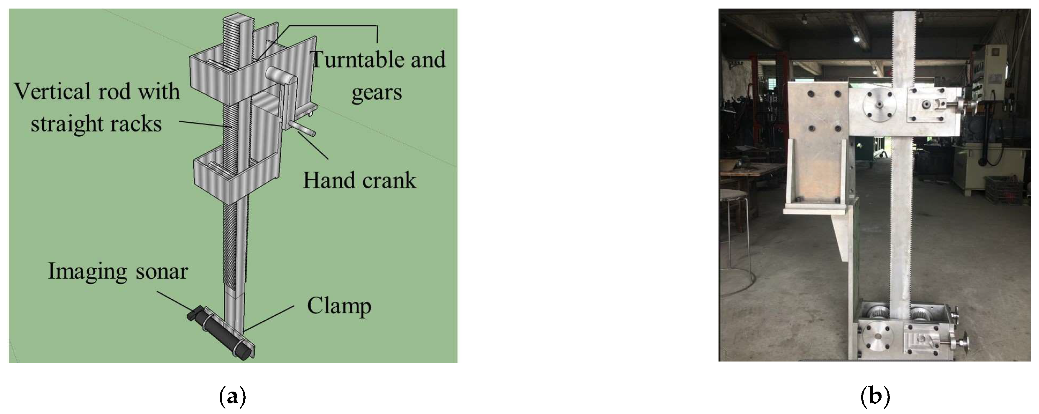
3.2. The Lifting Device to Carry the IS Device

The lifting device illustrated in Figure 6a consists of two parts: fixation installation and lifting equipment. The fixation installation is used to fix the IS device to the floating island. The lifting equipment contains a hand crank, a turntable, several interconnected gears, and a vertical rod with straight racks on both sides. The IS device is fixed at the end of the rod using a clamp. The hand crank can be rotated to turn the turntable while the internal gears rotate synchronously. Thereafter, the vertical rod with the IS device can be moved up and down through gear transmission.

Once the floating island is firmly attached to a pile, the lifting device can be rotated horizontally to position the IS device at a predesigned horizontal position. Subsequently, the IS device can descend to a predesigned height by moving the vertical rod. An initial prototype of the lifting device, which can deliver the IS device stably to a maximum depth of 13 m at a water speed of approximately 2.0 m/s in subsequent field tests, is shown in Figure 6b. Moreover, if the upper surface of the cap is above the water level, the lifting device can be placed on the surface for direct measurement.

3.3. Onsite Testing of the Platform

The aim of this test was to verify whether the platform could operate conveniently during the onsite scan.

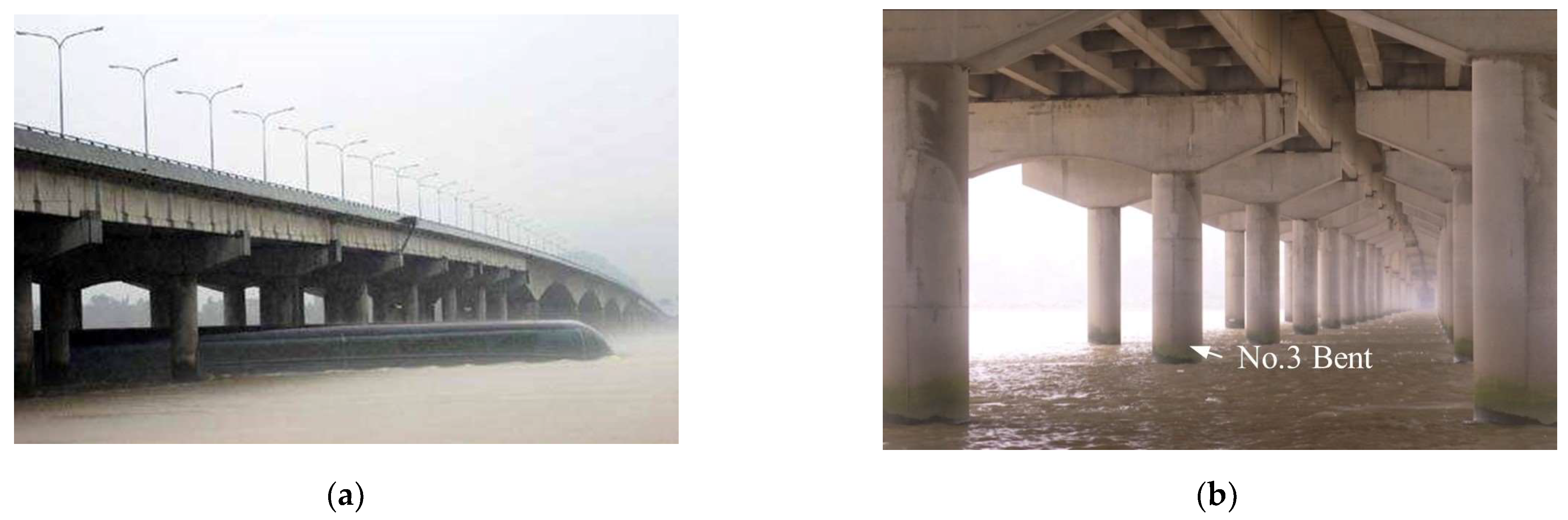
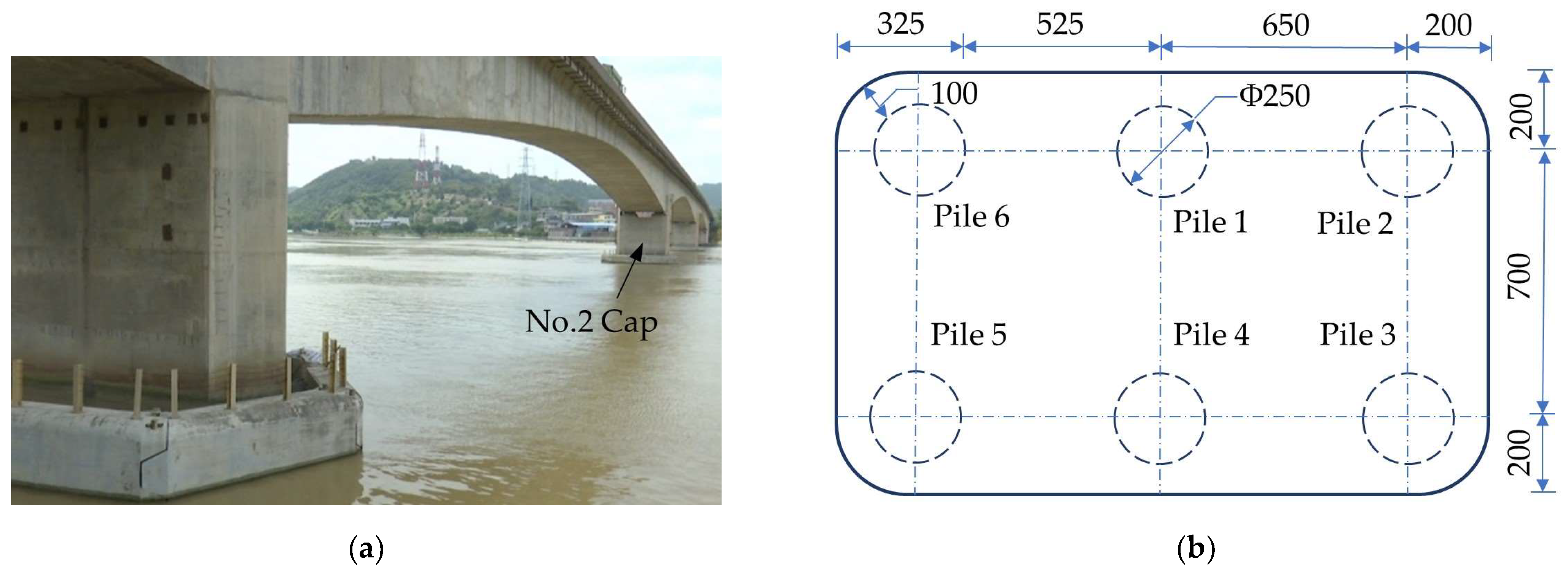
3.3.1. Overview of the Substructure of the Onsite Bridge

The Wulong River Highway Bridge, as shown in Figure 7, is a concrete T-beam bridge with a span arrangement of 29 × 20 m + 11 × 35 m + 3 × 110 m + 21 × 35 m that crosses the Wulong River in Fuzhou City, Fujian Province, China. Numerous two-column bents and concrete piles with uniform diameters of 1.5 m were used in the bridge substructure. The pile cap is submerged for most of the year. The No.3 bents, situated approximately 40 m from the shoreline of the river, were tested in this study.

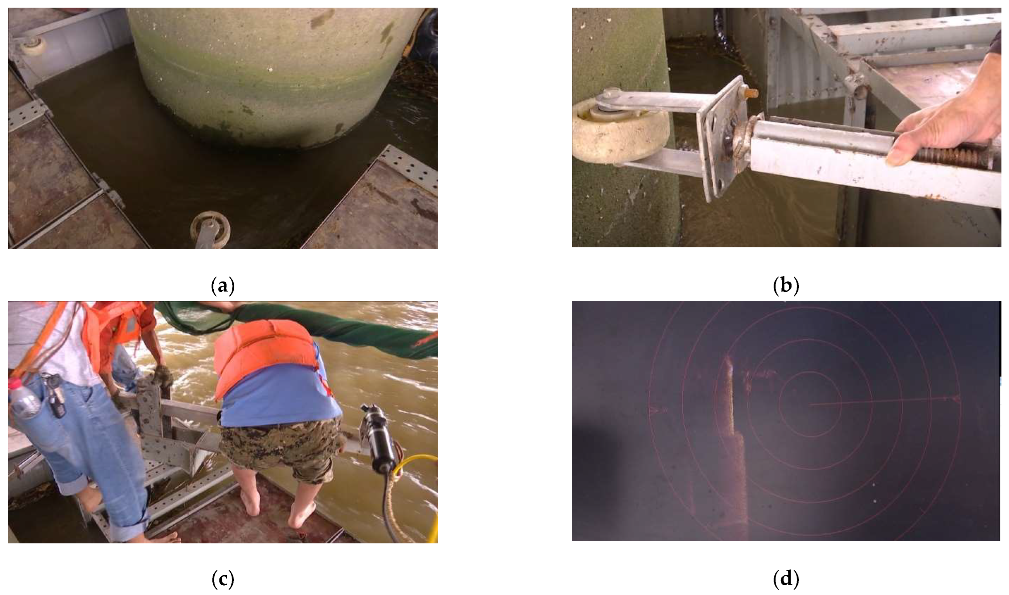
3.3.2. Test Procedure and Results

The test was conducted on 20 June 2019, which was the day with the highest astronomical tide. The current velocity in the test area was approximately 2.0 m/s. The yellow color of the river indicated a large amount of mud and sand. Prior to the test, 24 disassembled buoys and four length-adjustable rods were delivered by a pickup truck to the river shore. Each buoy was fabricated with a barrel and enclosed externally by a light metal frame. The procedure and duration of each test step are listed below. Figure 8 shows test steps III–VI.

Step I: All the buoys and rods were assembled into a floating island within a duration of approximately 40 min.

Step II: The floating island was driven by a ship closer to the pile. The time taken was approximately 5 min.

Step III: The floating island was divided into two parts and reconnected around the pile using bolts. The pile was positioned inside a formed hole.

Step IV: The length of each rod was adjusted to ensure that the end of each rod was against the pile surface. During this time, the pile was sandwiched between the floating islands. The duration of steps III and IV was approximately 20 min.

Step V: The lifting device was installed on the floating island and connected successively via five vertical rods to lower the IS device to a depth of 5 m. The duration was approximately 10 min.

Step VI: The pile was scanned within a duration of approximately 2 min.

Step VII: The floating island was rotated to move the IS device to another position.

Step VIII: The IS device was recovered, the floating island was divided, and the platform was taken back to the shore; the process took about 30 min.

Compared to inspections by divers or AUVs, several unique advantages of the platform were revealed in this test. Firstly, the preparation stage for the practical scan, composed of steps I–V, took approximately 1 h, which is equivalent to the preparation time for underwater inspector diving. Moreover, the platform was suitable for lengthy pile inspections, whereas an underwater inspector can only dive for a few hours per day. The next advantage concerns the safety and stability of inspections in strong currents. The sonar images of the underwater pile clearly demonstrated that the pile was intact, which was consistent with the results of the underwater detection by divers. This also proves that the platform was able to ensure a stable sonar scan under a flow rate of 3–4 knots. This high flow rate would pose a danger to the divers and AUVs. Thus, we concluded that the platform is suitable for underwater inspection in the case of extended periods, high flow rates, and muddy water environments.

4. Measuring Point Arrangement

Each measurement point contained one horizontal and one vertical position. The first three subsections discuss the horizontal arrangement of the sonar-scanning measurement points: Section 4.1 discusses the arrangement of the measurement points during the scanning of a single pile, Section 4.2 uses the extension method to move unreachable measurement points under the pile cap outside the cap, and Section 4.3 discusses the replacement of the unmovable measurement points. Section 4.4 discusses the vertical arrangement.

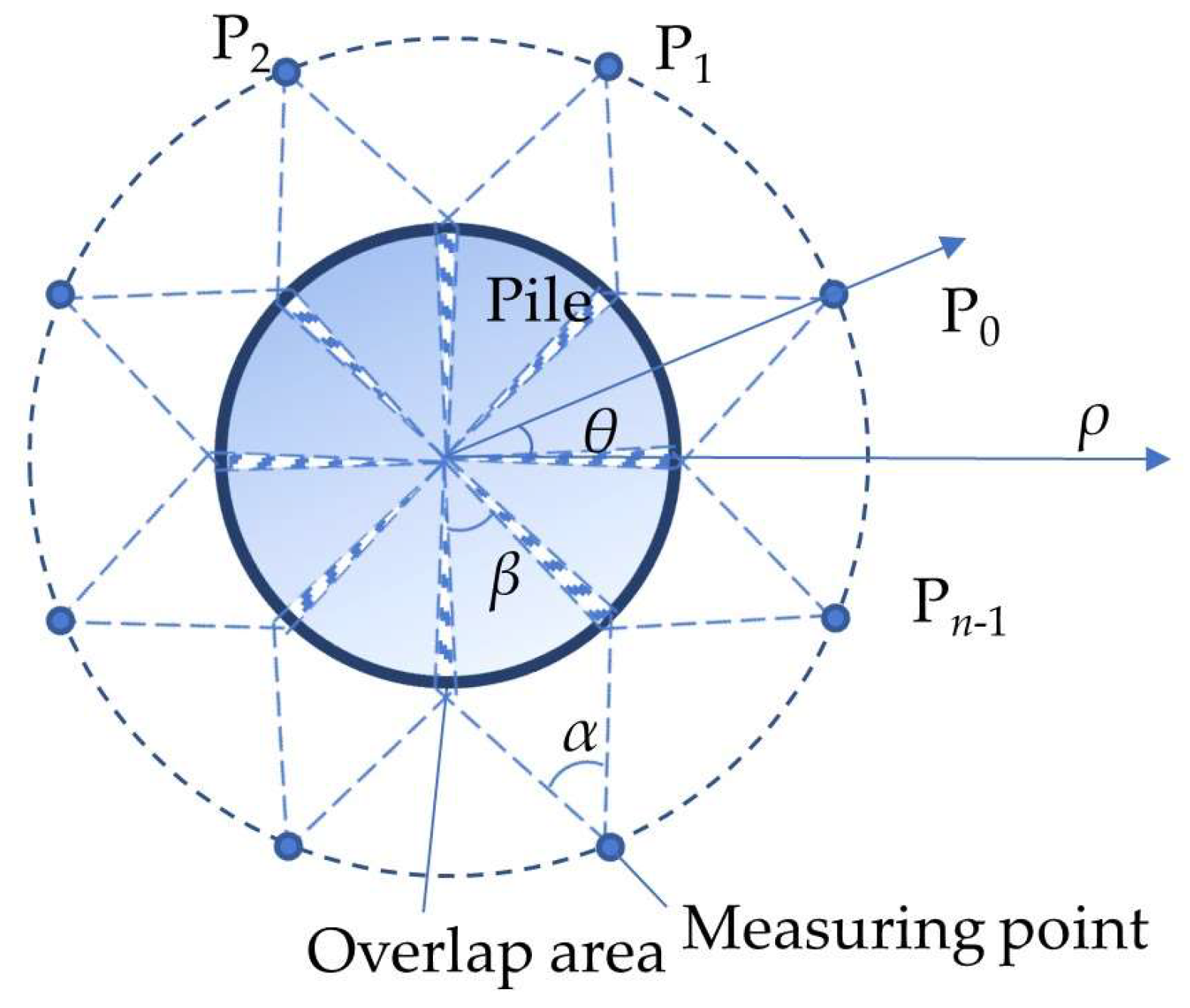
4.1. Absence of a Pile Cap

The pile cap is excluded in the case of a large-diameter cast-in-place pile. If the water level is significantly lower than the bottom of the cap, the influence of the pile cap on the IS scan can be ignored. The sonar can be placed at any position beyond the smallest distance, typically an approximate distance of 0.5 m from the instrument to the pile, to avoid image distortion.

As illustrated in Figure 9, α, β, r, and l represent the vertical beamwidth of the scan signal, the central angle of the horizontal scanning range, the radius of the pile, and the shortest distance between the IS device and pile edge, respectively. In Figure 9a, α₀ is the maximum horizontal beamwidth of IS, and it is also a predesigned value based on the IS performance. l₀ is the corresponding horizontal distance from the IS device to the pile edge. β₀ is equal to the supplementary angle of α₀. Thus, β₀/2 = π/2 − α₀/2. Therefore, the relationship between l₀ and r is as follows:

$$\left(r+l_0\right)\sin \left({\alpha }_0/2\right)=r$$

(1)

Based on Equation (1), l₀ is obtained as follows:

$$l_0=\left[\csc \left({\alpha }_0/2\right)-1\right]r$$

(2)

Considering that the scanning ranges of adjacent measuring points need to partially overlap, the number n₀ of the required measuring points is determined as follows:

$$n_0=\left\{\begin{array}{c}\mathrm{int}(2\pi /{\beta }_0)+1,0\le \mathrm{mod}(2\pi /{\beta }_0)<0.5\\ \mathrm{int}({2\pi /\beta }_0)+2,0.5\le \mathrm{mod}(2\pi /{\beta }_0)<1\end{array}\right.$$

(3)

where int () and mod () represent the integer- and fraction-valued functions, respectively. For 0 ≤ mod(2π/β₀) < 0.5, the total overlap area is relatively large, whereas for 0.5 ≤ mod(2π/β₀) < 1, the total overlap is relatively small. Thus, n₀ must be increased to increase the range of the overlap area.

If n₀ is significantly lower than the expected number determined from experience, both l and α need to be reduced. Figure 9b shows the relationship of α, r, and l for l ≤ l0 and α ≤ α₀. By pre-determining the appropriate values of l and α, Equation (4) exists based on the law of sines.

$$\frac{\sin \left(\pi -\alpha /2-\beta /2\right)}{r+l}=\frac{\sin \left(\alpha /2\right)}{r}$$

(4)

β is obtained as follows:

$$\beta =2\arcsin \left[\left(1+l/r\right)\sin \left(\alpha /2\right)\right]-\alpha$$

(5)

By substituting Equation (5) into Equation (6), the required number n of measuring points is obtained.

$$n=\left\{\begin{array}{c}\mathrm{int}(2\pi /\beta )+1,0\le \mathrm{mod}(2\pi /\beta )<0.5\\ \mathrm{int}(2\pi /\beta )+2,0.5\le \mathrm{mod}(2\pi /\beta )<1\end{array}\right.$$

(6)

If n₀ is significantly higher than the expected number determined from experience, l must be increased. Figure 9c shows the diagram of assuming l ≥ l₀. If l is preset, β is obtained as follows:

$$\beta =2\arccos \left[r/\left(r+l\right)\right]$$

(7)

By substituting Equation (7) into Equation (6), the required number n of measuring points for this study was acquired.

Figure 10 illustrates an arrangement of measuring points for a monopile without a cap based on the acquired α, β, l, and n. All points are distributed uniformly on the circle, which means that every point was at a uniform distance from the pile edge, and the center angle of the arc between the adjacent measuring points is equal. The center of the pile was assumed to be the original point of the polar coordinate system. The horizontal lines represent the polar axes. ρ and θ represent the polar radius and polar angle of any point in the system, respectively. Thus, the coordinates of the measuring points P₀–P_n−1 are (ρ₀, θ₀) − (ρ_n−1, θ_n−1). The center angle of each overlapping part is named φ. These parameters are derived as follows:

$${\rho }_i=r+l_i l_i=l (i=0,1,\cdots ,n-1)$$

(8)

$${\theta }_i=\left(2i+1\right)\pi /n (i=0,1,\cdots ,n-1)$$

(9)

$$\phi =\beta -\left(2\pi \right)/n$$

(10)

In most cases, the actual l is set to be less than l₀ generally for a monopile without a cap because the scan accuracy decreases with an increase in l.

4.2. Existence of a Pile Cap

Most pile cap arrangements can be summarized into four cases or combinations thereof: (a) a monopile, (b) four piles (2 × 2), (c) n piles arranged in a row, and (d) six piles (2 × 3). In addition, based on the experience from the laboratory and onsite tests, arranging 6–8 measuring points around a monopile is suitable for maintaining a balance between scan efficiency and precision. As the derivation of the 6-point case is similar to and easier than that of the 8-point case, the 8-point case is adopted in the following derivation.

4.2.1. A Monopile

Figure 11 shows that P₀ to P_n−1 must be moved outward from the original positions determined by the method proposed in Section 4.1 owing to the existence of the pile cap. For example, Point O was assumed to be the center of the horizontal cross section of the pile. Along the straight line OP₀, P₀ is moved outward to P’₀ just outside the cap edge. Accordingly, the distance between the point and pile edge increases from l to l′. The other points can then similarly be moved outward to their appropriate positions. Replacing l with l′ in Equations (5) and (10) can produce β′ and φ′.

4.2.2. Four Piles (2 × 2) in a Pile Cap

Owing to the existence of the pile cap shown in Figure 12, P₀, P₅, P₆, and P₇ must be moved outward to P′₀, P′₅, P′_6, and P′₇, respectively, which are located immediately outside the pile cap edge. Both P′₀ and P′₅ showed the same movement, whereas the other two points showed different movements.

Subcase 1: Movement of P′₀ and P′₅

The shape of the pile cap is assumed to be square, and each side length of the square is a. Four piles, named Piles 1–4, are uniformly distributed in the cap. All the piles are positioned at an identical distance p between the center point of the pile and the pile cap edge. The center point O of Pile 1 is defined as the original point, and the coordinate of P′₀ is given as (p/sinθ₀, θ₀) in the polar coordinate system. Point Q is assumed to be the center of the horizontal cross section of Pile 2. Points A and B represent the two ends of the overlapping range φ covered by two beams emitting from P′₀ and P′₇, respectively. Point C is the intersection of the straight-line BP’₇ and the line perpendicular to BP′₇ through point Q, and point D is the intersection of the straight-line AP’₀ and the line perpendicular to AP′₀ through point Q. Point M is the intersection of the straight lines OQ and AP′₀.

Based on the law of sines, Equation (11) is valid in ΔOP’₀A.

$$\frac{\sin \angle \mathrm{O}{\mathrm{P}}_0^{\prime }\mathrm{A}}{r}=\frac{\sin \left(\pi -\angle \mathrm{O}{\mathrm{P}}_0^{\prime }\mathrm{A}-{\theta }_0-\phi /2\right)}{p/\sin {\theta }_0}$$

(11)

The expression of ∠OP′₀A is derived as follows:

$$\angle O{P}_0^{\prime }A=\mathrm{arccot}\left[\frac{p}{r\cdot \sin ({\theta }_0+\phi /2)\cdot \sin {\theta }_0}-\cot ({\theta }_0+\phi /2)\right]$$

(12)

In ΔOP′₀M, Equation (13) is built similarly based on the law of sines.

$$\frac{\sin \angle \mathrm{O}{\mathrm{P}}_0^{\prime }\mathrm{M}}{\mathrm{OM}}=\frac{\sin \left(\pi -\angle \mathrm{O}{\mathrm{P}}_0^{\prime }\mathrm{M}-{\theta }_0\right)}{p/\sin {\theta }_0}$$

(13)

Then, the length of line segment OM is obtained as follows:

$$OM=\frac{\sin \angle O{P}_0^{\prime }M}{\sin (\angle O{P}_0^{\prime }M+{\theta }_0)}\cdot \frac{p}{\sin {\theta }_0}=\frac{\sin \angle O{P}_0^{\prime }A}{\sin (\angle O{P}_0^{\prime }A+{\theta }_0)}\cdot \frac{p}{\sin {\theta }_0}$$

(14)

Although Pile 2 can partially obstruct the transmission of the sound waves emitting from P’₀, the obstruction should not reduce φ. This requirement can be expressed using Equation (15).

$$\frac{\sin \angle O{P}_7^{\prime }B}{r}=\frac{\sin \left[\pi -\angle O{P}_7^{\prime }B-\left(2\pi -{\theta }_7+{\theta }_0/2\right)\right]}{\left(a-p\right)/\cos \left(2\pi -{\theta }_7\right)}$$

(15)

Thus, if Equation (15) is satisfied, the existence of the pile cap and Pile 2 will have no influence on the IS device placed at P′₀. By applying symmetry, analogous deductions can be made to derive the conditions that ensure that the pile cap and Pile 4 will not affect the IS device placed at P′_5.

Subcase 2: Movement of P′6 and P′7

In OP′₇B, Equation (16) is valid based on the law of sines.

$$\frac{\sin \angle O{P}_7^{\prime }B}{r}=\frac{\sin \left[\pi -\angle O{P}_7^{\prime }B-\left(2\pi -{\theta }_7+{\theta }_0/2\right)\right]}{\left(a-p\right)/\cos \left(2\pi -{\theta }_7\right)}$$

(16)

The expression of ∠OP’₇M is derived as follows.

$$\angle O{P}_7^{\prime }B=\mathrm{arccot}\left[\cot ({\theta }_7-\phi /2)-\frac{a-p}{r\sin ({\theta }_7-\phi /2)\cos {\theta }_7}\right]$$

(17)

In OP’₇M, Equation (18) is built similarly based on the law of sines.

$$\frac{\sin \angle O{P}_7^{\prime }M}{OM}=\frac{\sin \left[\pi -\angle O{P}_7^{\prime }M-\left(2\pi -{\theta }_7\right)\right]}{\left(a-p\right)/\cos \left(2\pi -{\theta }_7\right)}$$

(18)

The length of line segment OM is obtained as follows.

$$OM=\frac{\sin \angle O{P}_7^{\prime }M}{\sin (\angle O{P}_7^{\prime }M-{\theta }_7)}\cdot \frac{a-p}{\cos {\theta }_7}=\frac{\sin \angle O{P}_7^{\prime }B}{\sin (\angle O{P}_7^{\prime }B-{\theta }_7)}\cdot \frac{a-p}{\cos {\theta }_7}$$

(19)

Equation (20) expresses the condition for an IS device placed at P′7 to propagate its signal without being affected by the pile cap and pile 2. According to symmetry, the condition guaranteeing that the pile cap and Pile 3 do not affect the IS device placed at P’₆ and P′₅ can also be derived through an analogous deduction.

$$\begin{array}{l}r\le CQ=MQ\cdot \sin \angle P_7^{\prime }MQ=(OQ-OM)\cdot \sin (2\pi -{\theta }_7+\angle O{P}_7^{\prime }B)\\ =(OQ-OM)\cdot \sin (\angle O{P}_7^{\prime }B-{\theta }_7)\end{array}$$

(20)

4.2.3. N Piles Arranged in a Row in a Pile Cap

As shown in Figure 13, the proposed method can be used to verify the feasibility of measuring the point arrangement for N piles standing in a row in a pile cap. The point placement in Figure 13 is a typical extension of that in Figure 11 and Figure 12.

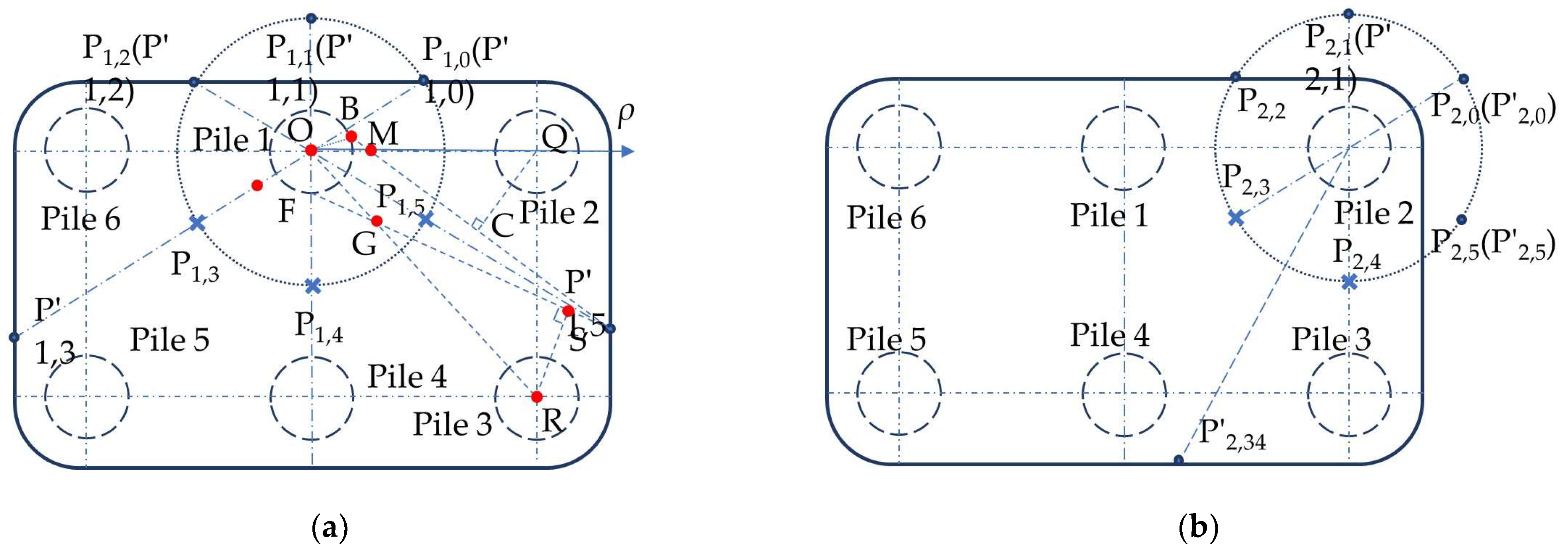
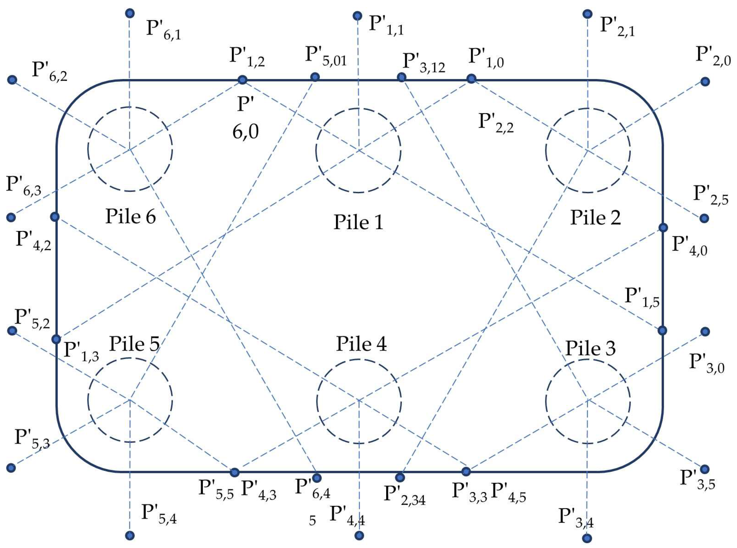
4.2.4. Six Piles (2 × 3) in a Pile Cap

Figure 14 shows the case of six piles arranged in two rows and three columns in a pile cap. All the measurement points are moved outwards to the outside of the pile cap edge. The movements of P₃ and P₄ are symmetrical to those of P₀ and P₇, respectively. The applicable conditions for these movements are the same as those in Equations (11)–(20).

For the case of more than six piles standing in more than two rows, the derivation of the feasibility of the measuring point arrangement is similar to that shown in Section 4.2.2.

4.3. Replacement of Unmovable Measuring Point

Although Section 4.2 proposes a method to move the point under the pile cap outward to the edge of the pile cap, the movements of some measuring points are inaccessible because they are blocked by neighboring piles. Figure 15a illustrates one unmovable point (P₄), and Figure 15b shows three unmovable points (P₀, P₇, and P₆). In these cases, a feasible solution is to replace the obstructed points with adjacent free points or additional points to guarantee that the scanning range remains unchanged.

4.3.1. Feasibility of Replacing One Point

As shown in Figure 16, the movement of P₄ is obstructed by Pile 4. Thus, the feasibility of placing an IS device at P′₅ to scan Pile 4 is given as follows: Points O and R represent the centers of the cross sections of Pile 1 and Pile 3, respectively. P₅ is moved outward to P′₅, located at the edge of the cap. The distance p from the center of the cross section to the edge of the cap is uniform for each pile, ranging from Pile 1 to Pile 4. F is the intersection of OP₄ and the pile surface, and G is the intersection between OR and FP′₅. S is the intersection of FP′_5, and the line perpendicular to FP′₅ through R. A polar coordinate system can be constructed for Pile 1, assuming the center O of Pile 1 is the original point, and the horizontal line is the polar axis. δ is the angle between OR and the polar axis. θ₄ and θ₅ represent the angular coordinates of P₄ and P₅, respectively. According to symmetry, the replacement is valid if the signal emitted from P′₅ can reach F without hindrance.

Based on the law of sines, Equation (21) is valid in ΔOP′₅F.

$$\frac{\sin \angle O{P}_5^{\prime }A}{r}=\frac{\sin \left(\pi -\angle O{P}_5^{\prime }F-\angle FO{P}_5^{\prime }\right)}{O{P}_5^{\prime }}$$

(21)

Substituting ∠FOP′₅ = θ₅ − θ₄, OP’₅ = (a − p)/cos(2π − θ₅) into Equation (21), ∠FOP′₅ is shown as follows:

$$\angle O{P}_5^{\prime }F=\mathrm{arccot}\left[\frac{a-p}{r\sin \left({\theta }_5-{\theta }_4\right)\cos {\theta }_5}-\cot \left({\theta }_5-{\theta }_4\right)\right]$$

(22)

In ΔOP′₅G, Equation (23) is built similarly based on the law of sines.

$$\frac{\sin \angle O{P}_5^{\prime }G}{OG}=\frac{\sin \angle P_5^{\prime }GO}{O{P}_5^{\prime }}$$

(23)

Substituting ∠P’₅GO = π − ∠OP’₅F − (θ₅ − δ) into Equation (23), the length of OG is obtained as follows:

$$OG=\frac{(a-p)\cdot \sin \angle O{P}_5^{\prime }F}{\cos {\theta }_5\cdot \sin (\angle O{P}_5^{\prime }F+{\theta }_5-\delta )}$$

(24)

To avoid signal transmission being obstructed by Pile 3, Equation (25) must be valid.

$$r\le SR=GR\cdot \sin \angle SGR=(OR-OG)\cdot \sin (\angle O{P}_5^{\prime }F+{\theta }_5-\delta )$$

(25)

4.3.2. Feasibility of Replacing More Than One Point

The replacement in Figure 17 is considered an example. Points O, Q, and R are the centers of the cross sections of Piles 1, 2, and 3, respectively. For each pile from Pile 1 to Pile 4, the distance p from the center of the cross section to the edge of the pile cap is uniform. B is the edge point of the scan beam emitted from P₀. ∠BOQ = θ₀ + β/2. P′₇₀ is the intersection of the bisector line of ∠P₇OP₀ and the pile cap edge. P′₆₇ is the intersection of the bisector line of ∠P₆OP₇ and the pile cap edge. C is the intersection of BP’₇₀ and the line perpendicular to BP′₇₀ through Q. E is the intersection of OP₇ and the edge of P₁. S is the intersection of EP′₇₀ and the line perpendicular to EP′₇₀ through R. M is the intersection of BP′₇₀ and OQ. θ₀ and θ₇ are the angular coordinates of P₀ and P₇, respectively.

Two conditions determine the availability of replacing P₀, P₆, and P₇ with P′₆₇ and P′₇₀. First, the scanning ranges of the IS device placed at P′₆₇ and P′₇₀ can cover those of the IS device placed at P₆ and P₀. Second, the scanning ranges of the IS device placed at P’₆₇ and P′₇₀ can cover those of the IS device placed at P₇. Because of symmetry, the above conditions are simplified as follows: (a) the scanning range of the IS device placed at P′₇₀ can cover the scanning range of the IS device placed at P₀, and (b) the scanning range of the IS device placed at P′₇₀ can cover the half-scanning range of the IS device placed at P₇.

• Feasibility of replacing P0 with P′₇₀

Based on the law of sines, Equation (26) is valid in ΔOP′₇₀B.

$$\frac{\sin \angle O{P}_{70}^{\prime }B}{r}=\frac{\sin \left(\pi -\angle O{P}_{70}^{\prime }B-\angle BO{P}_{70}^{\prime }\right)}{O{P}_{70}^{\prime }}$$

(26)

∠OP′₇₀B is derived by substituting ∠BOP′₇₀ = β/2 + (θ₀ + 2π − θ₇)/2 and OP′₇₀ = (a − p)/cos[(θ₀ + 2π − θ₇)/2] into Equation (26).

$$\angle O{P}_{70}^{\prime }B=\mathrm{arccot}\left[\frac{a-p}{r\sin ({\theta }_7/2-{\theta }_0/2-\beta /2)\cos ({\theta }_7/2-{\theta }_0/2)}+\cot ({\theta }_7/2-{\theta }_0/2-\beta /2)\right]$$

(27)

In OP′₇₀M, Equation (28) is built similarly based on the law of sines.

$$\frac{\sin \angle \mathrm{O}{\mathrm{P}}_{70}^{\prime }B}{OM}=\frac{\sin \angle {\mathrm{P}}_{70}^{\prime }MO}{\mathrm{O}{\mathrm{P}}_{70}^{\prime }}$$

(28)

Substituting ∠P′₇₀MO = π − ∠OP’₇₀B − (θ₀ + 2π − θ₇)/2 into Equation (28), OM is obtained as follows:

$$OM=\frac{(a-p)\cdot \sin \angle O{P}_{70}^{\prime }B}{\cos ({\theta }_7/2-{\theta }_0/2)\cdot \sin ({\theta }_7/2-{\theta }_0/2-\angle O{P}_{70}^{\prime }B)}$$

(29)

Equation (30) expresses the requirement for an IS device placed at P′₇₀ to propagate its signal unaffected by the pile cap and pile 2.

$$r\le CQ=MQ\cdot \sin \angle CMQ=(OQ-OM)\cdot \sin [\angle O{P}_{70}^{\prime }B+({\theta }_0+2\pi -{\theta }_7)/2]$$

(30)

2.

Feasibility of replacing P₇ with P′₇₀

Based on the law of sines, Equation (31) is valid in ΔOP′₇₀E.

$$\frac{\sin \angle O{P}_{70}^{\prime }E}{r}=\frac{\sin \left(\pi -\angle EO{P}_{70}^{\prime }-\angle O{P}_{70}^{\prime }E\right)}{O{P}_{70}^{\prime }}$$

(31)

Substituting ∠EOP′₇₀ = (θ₀ + 2π − θ₇)/2 and OP’₇₀ = (a − p)/cos[(θ₀ + 2π − θ₇)/2] into Equation (31), ∠OP′₇₀E is obtained as follows:

$$\angle \mathrm{O}{\mathrm{P}}_{70}^{\prime }\mathrm{E}=\mathrm{arccot}\left[\frac{2(a-p)}{r\sin ({\theta }_7-{\theta }_0)}-\cot ({\theta }_7/2-{\theta }_0/2)\right]$$

(32)

If Equation (33) is valid, half the scanning range of the IS device at P₇ can be covered by that at P′₇₀. Thus, Pile 3 does not affect the replacement scan.

$$r\le SR=ER\cdot \sin \angle SER=\left[\sqrt{2}(a-2p)-r\right]\cdot \sin (\angle EO{P}_{70}^{\prime }+\angle O{P}_{70}^{\prime }E)$$

(33)

According to symmetry, the conditions to ensure that the measurement point P₆ can be replaced by P′₆₇ are similarly deduced.

These deductions prove that replacing the obstructed points with adjacent free points, adding new measuring points, or combining the two methods can avoid the obstruction of signal propagation caused by adjacent piles and pile caps. However, it must be pointed out that Equations (21)–(33) are not applicable to every practical case because the sizes of the pile cap and piles and the arrangement of the piles in the HRPCF may differ for different bridges. The conditional equations for feasible replacement need to be rebuilt based on derivations similar to that in Section 4.3.1 and Section 4.3.2.

4.4. Layout of the Vertical Position of the Measuring Point

As shown in Figure 18, the distance between the IS device and pile edge is l, and the scanning range of IS is R. Therefore, the vertical range h of the scanning range on the pile surface can be approximated as follows:

$$h=2\sqrt{R^2-l^2}=2l\tan \omega$$

(34)

where ω represents the angle between R and l.

If the total length of the pile exposed to water is L, m times the number of horizontal measuring points is required in the vertical direction.

$$m=\mathrm{int}(L/h)+1=\mathrm{int}(L/(2l\tan \omega ))+1$$

(35)

When the locations of the measurement points around each pile are determined, a new 3D Cartesian coordinate system for the total pile group can be built, and the coordinates of each point in the initial polar coordinate system can be transformed into a 3D Cartesian coordinate system.

5. Onsite Test for the Proposed Arrangement of Measuring Points

The main purpose of this test was to verify the applicability of the proposed IS measuring point arrangement for inspecting underwater HRPCFs.

5.1. Overview of the Substructure of an Onsite Bridge

The Wulong River New Bridge, as shown in Figure 19a, is a prestressed concrete box-girder bridge used for heavy-haul transportation. The bridge span is divided into six parts: 31, 49, 3 × 144, and 86 m, with five hollow concrete piers. The foundation of the bridge is an HRPCF composed of a pile group (2 × 3) and a rectangular cap. The sizes and arrangements of the piles and pile caps under each pier were uniform, as shown in Figure 19b.

Pile cap No. 2 and its connected piles, at an approximate distance of 80 m from the shore, were used for this test. The underwater length of each pile was approximately 13 m. The floating island was fixed to the edge of the pile cap, and the distance between the outer edge of the floating island and the pile cap did not exceed 2 m. The IS and parameter configurations used in this test were the same as those described in Section 3.3.

The two features of the sonar images obtained from the onsite experiment can be used to test whether the proposed measuring point arrangement is applicable for underwater HRPCF inspection.

5.2. Arrangement of the Measuring Points

Substituting r = 1.25 m and α = 28° into Equation (2) gave l₀ = 3.92 m and n₀ = 3. The scan accuracy decreased due to insufficient measurement points. Thus, based on experience, n was increased to six. The maximum value of l was calculated as 2 + (2 − 1.25) = 2.75 m. Substituting l = 2.75 m into Equations (5), (6), and (10) gave β = 73.43°, n = 6, and φ = 13.43°. Six points, P_1,0–P_1,5, around Pile 1, were placed as shown in Figure 17a. P_1,0, P_1,1, and P_1,2 coincided with P′_1,0, P′_1,1, and P′_1,2, respectively. However, because P_1,3, P_1,4, and P_1,5 were just under the pile cap, they had to be replaced by P′_1,3 and P′_1,5. The feasibility of this replacement will be discussed in the following section. Because of the symmetry, the proof was simplified as follows: (a) the scanning range of the IS device placed at P′_1,5 covered the scanning range of the IS device placed at P_1,5, and (b) the scanning range of the IS device placed at P′_1,5 covering half the scanning range of the IS device placed at P_1,4. A polar coordinate system for Pile 1 was constructed; the center O of Pile 1 was assumed to be the original point, and the horizontal line was considered the polar axis. Thus, the coordinates of P_1,4 and P_1,5 were (4, 270°) and (4, 330°), respectively. The definitions of points B, M, C, F, G, S, and R in Figure 20a are the same as those in Figure 16 and Figure 17 (δ = 312.88° and OR = 9.55 m).

According to Equation (17), ∠OP′_1,5B is calculated as follows:

$$\begin{array}{l}\angle \mathrm{O}{\mathrm{P}}_{1,5}^{\prime }\mathrm{B}=\mathrm{arccot}\left[\cot ({\theta }_5-\phi /2)-\frac{a-p}{r\sin ({\theta }_5-\phi /2)\cos {\theta }_5}\right] \\ =\mathrm{arccot}\left[\cot (330°-13.43°/2)-\frac{8.5}{1.25\times \sin (330°-13.43°/2)\times \cos 330°}\right]\approx 4.85°\end{array}$$

(36)

Based on Equation (19), the length of OM is shown to be as follows:

$$OM=\frac{\sin \angle O{P}_{1,5}^{\prime }B}{\sin (\angle O{P}_{1,5}^{\prime }B-{\theta }_5)}\cdot \frac{a-p}{\cos {\theta }_5}=\frac{\sin 4.85°}{\sin (4.85°-330°)}\times \frac{8.5}{\cos 330°}=1.45 m$$

(37)

Thus, the scanning range of the sonar placed at P’_1,5 could cover the scanning range of the IS device placed at P_1,5. Equation (33) is proven to be valid by the following calculation.

$$r=1.25\mathrm{m}<(\mathrm{OQ}-\mathrm{OM})\cdot \sin (\angle \mathrm{O}{\mathrm{P}}_{1,5}^{\prime }\mathrm{B}-{\theta }_7)=(6.5-1.45)\times \sin (4.85°-330°)=2.89\mathrm{m}$$

(38)

According to Equation (22), ∠OP′_1,5F is calculated as follows:

$$\begin{array}{l}\angle O{P}_{1,5}^{\prime }F=\mathrm{arccot}\left[\frac{a-p}{r\sin \left({\theta }_5-{\theta }_4\right)\cos {\theta }_5}-\cot \left({\theta }_5-{\theta }_4\right)\right]\\ =\mathrm{arccot}\left[\frac{8.5}{1.25\times \sin (330°-270°)\times \cos 330°}-\cot (330°-270°)\right]\approx 6.72°\end{array}$$

(39)

Based on Equation (19), the length of OG is calculated as follows:

$$OG=\frac{(a-p)\cdot \sin \angle O{P}_{1,5}^{\prime }F}{\cos {\theta }_5\cdot \sin (\angle O{P}_{1,5}^{\prime }F+{\theta }_5-\delta )}=\frac{8.5\times \sin 6.72°}{\cos 330°\times \sin (6.72°+330°-312.88°)}=2.84m$$

(40)

Thus, the scanning range of the sonar placed at P′_1,5 covered half the scanning range of the IS device placed at P_1,4. Equation (41) is proven to be valid by the following calculation.

$$\begin{array}{l}r=1.25m<(OR-OG)\cdot \sin (\angle O{P}_5^{\prime }F+{\theta }_5-\delta )\\ =(9.55-2.84)\times \sin (6.72°+330°-312.88°)=2.71m\end{array}$$

(41)

Furthermore, based on the method proposed in Section 4.2 and Section 4.3, the horizontal positions of the measurement points for Pile 2 were similarly determined, as shown in Figure 20b. Figure 21 illustrates the horizontal placement of the 30 measuring points for Piles 1–6 in pile cap No. 2.

Substituting L = 13 m, l = 2.75 m, and ω = 50° into Equation (35) gave m = 2.

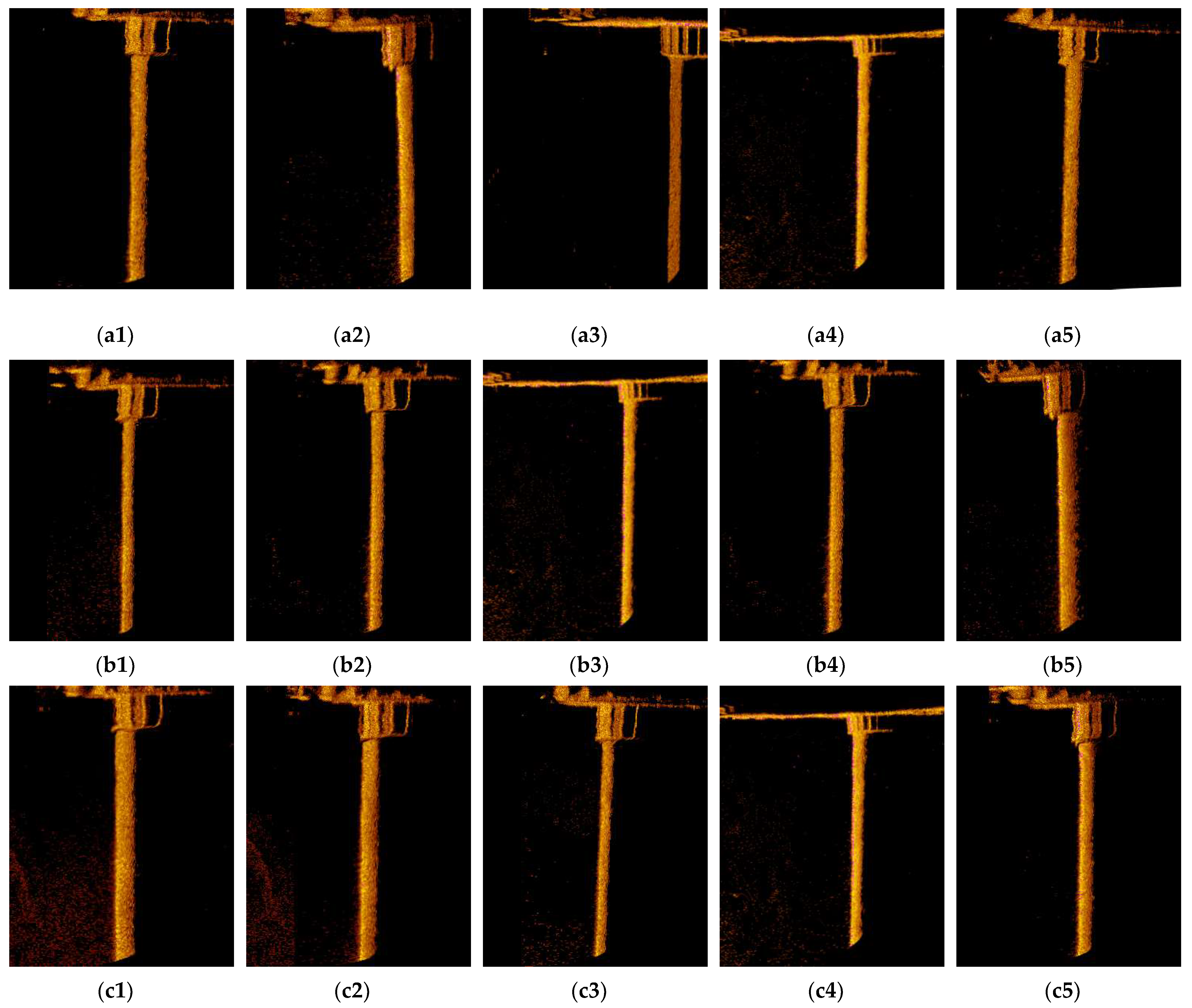
5.3. Analysis of the Obtained Images

The layouts of the measuring points of Piles 1, 2, and 6 were completely symmetrical with Piles 3, 4, and 5. Therefore, the images of Piles 1, 2, and 6 were sufficient to analyze whether the adjacent piles obstructed signal propagation. Figure 22 shows an image obtained from the IS device placed at each measuring point on Piles 1, 2, and 6. Three objects, including the pile, the steel frame around the top of the pile, and the base plate of the pile cap, were observed in each image. The red points in each image represent the measurement points. Figure 22(a1–a5) show the five images obtained from the IS device placed at the measuring points P′_1,0–P′_1,5. Scan distance l in Figure 22(a3,a4) was longer than that in the other images, which was consistent with the proportion of the scan distance corresponding to the different positions shown in Figure 21. A similar characteristic can be observed in the sonar images in Figure 22(b1–b5,c1–c5). In addition, two features of the sonar images obtained from the onsite experiment demonstrated the applicability of the proposed measuring point arrangement for underwater HRPCF inspection. First, no echo signals, except for the echo signal from the tested pile within the scanning range of every image, were detected. Second, the echo signal from the outer surface of the tested pile in each image was intact. These features indicate that the adjacent piles are far from the scanning range of the sonar placed at any preset measuring point. The signal and echo signals were unobstructed during emission and reflection. Thus, the proposed IS measuring point placement is verified to be effective in the current case.

6. Conclusions

This paper presents the state of the measuring point arrangement of IS for underwater HRPCF inspection based on an assembled sonar-carried platform. The major contributions of this study are as follows.

• The appropriate preset value ranges of two key parameters for the design of measuring point placement, including the horizontal measuring distance l and the pitch angle ω, are experimentally summarized as 1.0 m ≤ l ≤ 3.0 m and 0° ≤ ω ≤ 50°.
• The proposed assembled sonar-carried platform can provide a 13 m deep stable scan in a strong current with a flow speed close to 2.0 m/s. This provides a feasible alternative for solving the problem of unstable scans by AUVs in strong currents.
• Theoretical derivations and onsite tests show that the obstruction of the sonar signal by adjacent piles can be avoided by moving outward, adding, and replacing the obstructed measuring points. The obtained measuring point arrangement is helpful for the IS to scan the entire surface of each pile in the pile group without obstruction.

7. Scope for Future Research

In this study, we provide a solution for scanning underwater structures of bridges using imaging sonar. The proposed method is still mostly performed manually, and automation is the ultimate goal, for which additional and developed technologies are necessary. In the image acquisition phase, we need to investigate scanning solutions for other defects of underwater bridge components and develop automatic planning cruises for sonar platform movement trajectories; in the image analysis phase, we are developing automatic identification techniques for sonar images, and in the bridge repair phase, rapid repair methods for underwater structures are being developed.

In the future, the fully automated sonar inspection of underwater bridge structures will improve the efficiency of inspection, shorten the cycle of bridge inspections, timely detection, and timely repair, and finally achieve the goal of extending the service life of bridges.

References

1. Zhao, X.; Gong, X.; Duan, Y.; Guo, P. Load-Bearing Performance of Caisson-Bored Pile Composite Anchorage Foundation for Long-Span Suspension Bridge: 1-g Model Tests. Acta Geotech. 2023, 1–21. [Google Scholar] [CrossRef]
2. Avent, R.R.; Alawady, M.; Guthrie, L. Underwater Bridge Deterioration and the Impact of Bridge Inspection in Mississippi. Transp. Res. Rec. 1997, 1597, 52–60. [Google Scholar] [CrossRef]
3. Avent, R.R.; Alawady, M. Bridge Scour and Substructure Deterioration: Case Study. J. Bridge Eng. 2005, 10, 247–254. [Google Scholar] [CrossRef]
4. Sweeney, R.A.P.; Unsworth, J.F. Bridge Inspection Practice: Two Different North American Railways. J. Bridge Eng. 2010, 15, 439–444. [Google Scholar] [CrossRef]
5. Browne, T.M.; Collins, T.J.; Garlich, M.J.; O’Leary, J.E.; Stromberg, D.G.; Heringhaus, K.C. Underwater Bridge Inspection; United States, 2010; p. 54. Available online: https://rosap.ntl.bts.gov/view/dot/44391 (accessed on 12 March 2023).
6. Stromberg, D.G. New Advances in Underwater Inspection Technologies for Railway Bridges over Water. Railw. Track Struct. 2011, 107, 1–29. [Google Scholar]
7. Zhang, X.F.; Li, Q.N.; Ma, Y.; Jia, Y.S. Dimensional Imaging Sonar Damage Identification Technology Research On Sea-Crossing Bridge Main Pier Pile Foundations. In Proceedings of the 2016 5th International Conference on Energy and Environmental Protection (ICEEP 2016), Shenzhen, China, 17–18 September 2016. [Google Scholar]
8. Mueller, C.A.; Fromm, T.; Buelow, H.; Birk, A.; Garsch, M.; Gebbeken, N. Robotic Bridge Inspection within Strategic Flood Evacuation Planning. In Proceedings of the OCEANS 2017, Aberdeen, UK, 19–22 June 2017. [Google Scholar]
9. Hou, S.T.; Jiao, D.; Dong, B.; Wang, H.C.; Wu, G. Underwater Inspection of Bridge Substructures Using Sonar and Deep Convolutional Network. Adv. Eng. Inf. 2022, 52, 101545. [Google Scholar] [CrossRef]
10. Zheng, S.W.; Xu, Y.J.; Cheng, H.Q.; Wang, B.; Lu, X.J. Assessment of Bridge Scour in the Lower, Middle, and Upper Yangtze River Estuary with Riverbed Sonar Profiling Techniques. Environ. Monit. Assess. 2018, 190, 15. [Google Scholar] [CrossRef] [PubMed]
11. Murphy, R.R.; Steimle, E.; Hall, M.; Lindemuth, M.; Trejo, D.; Hurlebaus, S.; Medina-Cetina, Z.; Slocum, D. Robot-Assisted Bridge Inspection. J. Intell. Robot Syst. 2011, 64, 77–95. [Google Scholar] [CrossRef]
12. Topczewski, Ł.; Cieśla, J.; Mikołajewski, P.; Adamski, P.; Markowski, Z. Monitoring of Scour Around Bridge Piers and Abutments. Transp. Res. Procedia 2016, 14, 3963–3971. [Google Scholar] [CrossRef] [Green Version]
13. Clubley, S.; Manes, C.; Richards, D. High-Resolution Sonars Set to Revolutionise Bridge Scour Inspections. Proc. Inst. Civ. Eng. -Civ. Eng. 2015, 168, 35–42. [Google Scholar] [CrossRef] [Green Version]
14. Fadool, J.C.; Francis, G.; Clark, J.E.; Liu, G.; De Brunner, V. Robotic Device for 3D Imaging of Scour Around Bridge Piles. In Proceedings of the ASME International Design Engineering Technical, Chicago, IL, USA, 12–15 August 2013. [Google Scholar]
15. Shi, P.F.; Fan, X.N.; Ni, J.J.; Wang, G.R. A Detection and Classification Approach for Underwater Dam Cracks. Struct. Health Monit. 2016, 15, 541–554. [Google Scholar] [CrossRef]
16. Shi, P.F.; Fan, X.N.; Ni, J.J.; Khan, Z.; Li, M. A Novel Underwater Dam Crack Detection and Classification Approach Based on Sonar Images. PLoS ONE 2017, 12, e0179627. [Google Scholar] [CrossRef] [PubMed] [Green Version]
17. Chen, B.; Yang, Y.; Zhou, J.; Zhuang, Y.Z.; McFarland, M. Damage Detection of Underwater Foundation of a Chinese Ancient Stone Arch Bridge via Sonar-Based Techniques. Measurement 2021, 169, 108283. [Google Scholar] [CrossRef]
18. Helminen, J.; Dauphin, G.J.R.; Linnansaari, T. Length Measurement Accuracy of Adaptive Resolution Imaging Sonar and a Predictive Model to Assess Adult Atlantic Salmon (Salmo Salar) into Two Size Categories with Long-Range Data in a River. J. Fish Biol. 2020, 97, 1009–1026. [Google Scholar] [CrossRef]
19. Wei, B.; Li, H.S.; Zhou, T.; Xing, S.Y. Obtaining 3D High-Resolution Underwater Acoustic Images by Synthesizing Virtual Aperture on the 2D Transducer Array of Multibeam Echo Sounder. Remote Sens. 2019, 11, 2615. [Google Scholar] [CrossRef] [Green Version]
20. Burwen, D.L.; Fleischman, S.J.; Miller, J.D. Accuracy and Precision of Salmon Length Estimates Taken from DIDSON Sonar Images. Trans. Am. Fish. Soc. 2010, 139, 1306–1314. [Google Scholar] [CrossRef]
21. Daroux, A.; Martignac, F.; Nevoux, M.; Bagliniere, J.L.; Ombredane, D.; Guillard, J. Manual Fish Length Measurement Accuracy for Adult River Fish Using an Acoustic Camera (DIDSON). J. Fish Biol. 2019, 95, 480–489. [Google Scholar] [CrossRef]
22. Cook, D.; Middlemiss, K.; Jaksons, P.; Davison, W.; Jerrett, A. Validation of of Fish Length Estimations from a High Frequency Multi-Beam Sonar (ARTS) and Its Utilisation as a Field-Based Measurement Technique. Fish Res. 2019, 218, 59–68. [Google Scholar] [CrossRef]
23. Carreras, M.; David Hernandez, J.; Vidal, E.; Palomeras, N.; Ribas, D.; Ridao, P. Sparus II AUV-A Hovering Vehicle for Seabed Inspection. IEEE J. Ocean. Eng. 2018, 43, 344–355. [Google Scholar] [CrossRef]
24. Zhang, H.W.; Zhang, S.T.; Wang, Y.H.; Liu, Y.H.; Yang, Y.N.; Zhou, T.; Bian, H.Y. Subsea Pipeline Leak Inspection by Autonomous Underwater Vehicle. Appl. Ocean Res. 2021, 107, 102321. [Google Scholar] [CrossRef]
25. Zacchini, L.; Franchi, M.; Ridolfi, A. Sensor-Driven Autonomous Underwater Inspections: A Receding-Horizon RRT-Based View Planning Solution for AUVs. J. Field Robot. 2022, 39, 499–527. [Google Scholar] [CrossRef]
26. Song, Y.; He, B.; Liu, P. Real-Time Object Detection for AUVs Using Self-Cascaded Convolutional Neural Networks. IEEE J. Ocean. Eng. 2021, 46, 56–67. [Google Scholar] [CrossRef]
27. Dai, G.B.; Ji, G.Y. Optimization of Measurement Point Layout for Large Size Structures. Noise Vib. Control. 2015, 35, 185–190+206. [Google Scholar]
28. Ruan, J.A.; Li, C.J.; Li, M.; Wang, M.; Sun, F.; Lu, Y.Q. Determination of Safety Early Warning Value of Underwater Shield Tunnel Structural Health Monitoring Based on Probability Statistical Method. Saf. Environ. Eng. 2022, 29, 147–155. [Google Scholar]
29. Lança, R.; Fael, C.; Maia, R.; Pêgo, J.P.; Cardoso, A.H. Clear-Water Scour at Pile Groups. J. Hydraul. Eng. 2013, 139, 1089–1098. [Google Scholar] [CrossRef]
30. Amini, A.; Parto, A.A. 3D Numerical Simulation of Flow Field around Twin Piles. Acta Geophys. 2017, 65, 1243–1251. [Google Scholar] [CrossRef]
Figure 1. Schematic diagram of HRPCF and scanning: (a) pile group; (b) layout of measurement points placement.
Sustainability 15 06402 g001
Figure 2. Experiment design and operation: (a) design and manufacture of columns with spalling; (b) locations of IS device and columns.
Sustainability 15 06402 g002
Figure 3. Measured depth (dm) of spalling from the obtained sonar image: (a) dm = 51 mm (d = 50 mm, l = 1.5 m, ω = 10°); (b) dm is not measurable (d = 10 mm, l = 0.75 m, ω = 20°).
Sustainability 15 06402 g003
Figure 4. Values of dm for different values of l and ω: (a1) d = 50 mm, l = 0.5 m and 0.75 m; (a2) d = 50 mm, l = 1.0 m to 3.0 m; (a3) d = 50 mm, l = 3.5 m to 5.0 m; (b1) d = 40 mm, l = 0.5 m and 0.75 m; (b2) d = 40 mm, l = 1.0 m to 3.0 m; (b3) d = 40 mm, l = 3.5 m to 5.0 m; (c1) d = 30 mm, l = 0.5 m and 0.75 m; (c2) d = 30 mm, l = 1.0 m to 3.0 m; (c3) d = 30 mm, l = 3.5 m and 4.0 m; (d1) d = 20 mm, l = 0.5 m and 0.75 m; (d2) d = 20 mm, l = 1.0 m to 3.0 m; and (d3) d = 20 mm, l = 3.5 m.
Sustainability 15 06402 g004
Figure 5. Trial-produced prototype of the assembled floating island: (a) 3D sketch of the design; (b) photo of the trial-produced prototype.
Sustainability 15 06402 g005
Figure 6. Trial-produced prototype of the lifting device: (a) 3D sketch of the design; (b) photo of a trial-produced prototype.
Sustainability 15 06402 g006
Figure 7. Photos of the Wulong River Highway Bridge: (a) overview of the bridge; (b) the No.3 Bent.
Sustainability 15 06402 g007
Figure 8. Photo of step III to step VII of the test: (a) step III; (b) step IV; (c) step V; and (d) step VI.
Sustainability 15 06402 g008
Figure 9. Relationships between α, r, and l: (a) l = l0; (b) ll0 and αα0; and (c) l > l0 and αα0.
Sustainability 15 06402 g009
Figure 10. Distribution of measuring points for a monopile without a cap.
Sustainability 15 06402 g010
Figure 11. Arrangement of measuring points for a monopile in a pile cap.
Sustainability 15 06402 g011
Figure 12. Arrangement of measuring points for four piles (2 × 2) in a pile cap.
Sustainability 15 06402 g012
Figure 13. Arrangement of measuring points for N piles arranged in a row in a pile cap.
Sustainability 15 06402 g013
Figure 14. Measuring point placement for six piles (2 × 3) in a pile cap.
Sustainability 15 06402 g014
Figure 15. Few points that cannot be moved outward: (a) one unmovable point; (b) three unmovable points.
Sustainability 15 06402 g015
Figure 16. Replacement of one obstructed point.
Sustainability 15 06402 g016
Figure 17. Replacement of more than one point.
Sustainability 15 06402 g017
Figure 18. Layout of the vertical position of the measuring points.
Sustainability 15 06402 g018
Figure 19. Details of the substructure of the Wulong River New Bridge: (a) photo of the bridge; (b) sizes and arrangement of the piles in the No. 2 pile cap (unit: cm).
Sustainability 15 06402 g019
Figure 20. Measuring point placement: (a) Pile 1; (b) Pile 2.
Sustainability 15 06402 g020
Figure 21. Entire horizontal placement of 30 measuring points for 6 piles in the No. 2 pile cap.
Sustainability 15 06402 g021
Figure 22. Obtained images: (a1) P′1,1; (a2) P′1,2; (a3) P′1,3; (a4) P′1,5; (a5) P′1,0; (b1) P′2,1; (b2) P′2,2; (b3) P′2,34; (b4) P′2,5; (b5) P′2,0; (c1) P′6,1; (c2) P′6,2; (c3) P′6,3; (c4) P′6,45; and (c5) P′6,0.
Sustainability 15 06402 g022