A Hybrid Optimization Method for Sustainable and Flexible Design of Supply–Production–Distribution Network in the Physical Internet

Abstract

The resilience and sustainability of supply chains are facing new challenges due to the increasing complexity of supply chains. Compared to traditional supply chain networks, the Physical Internet (PI) has the potential to address sustainable development challenges and build resilient supply chain networks by providing interconnected and open logistics services. However, the interplay between resilience and sustainability has yet to be thoroughly explored in the PI-enabled supply chain literature. This paper aims to investigate the relationship between resilience and sustainability in PI-enabled supply chains. An innovative hybrid approach that combines the resilient-sustainable performance scoring method with mixed-possibilistic programming is proposed to trade-off and analyze the relationship between the two. Applying the concepts of resilience and sustainability to PI-enabled supply chains involves optimizing costs, sustainable performance, and resilience levels simultaneously. This enables coping with unforeseen disruptions from suppliers, plants, and PI hubs. The results of computational experiments have demonstrated that the PI-enabled supply chain exhibits stronger sustainable and resilience performance in dealing with random disruptions compared to traditional supply chains. The fruitful research yielded important management insights and practical implications, thereby contributing to the reinforcement of the literature on PI.

1. Introduction

In today’s globalized and increasingly volatile environment, supply chains are becoming more complicated due to multiple links, independent participants, and global supply and demand relationships. Due to supply chain complexity, many events threaten operations and jeopardize performance and stability [1,2]. Thus, avoiding and mitigating the impact of risks can be very challenging. Academics have conducted research on supply chain risks from multiple perspectives. Supply chain risk is subdivided into operational risk and disruption risk, with the latter typically resulting from external factors such as natural disasters and accidents. For example, Erickson caused a shortage of key parts due to firing a supplier in 2000, resulting in an economic loss of EUR 400 million [3]. In 2001, Land Rover experienced a shortage of key components due to a major supplier’s bankruptcy, resulting in the termination of 1400 employees [4]. In response to disruptions, various risk mitigation strategies have been explored in the literature, such as information sharing [5], buffer inventory [6,7], contracts with backup suppliers, multi-source procurement [8,9,10], etc. Nevertheless, some of these mitigating factors enhance the resilience and flexibility of the supply chain, which may not be the best option from a sustainable perspective [11]. To be competitive, companies have to make a proper balance between resilience and sustainability [10,12,13].

Recently, researchers have devoted considerable attention to exploring the relationship between the resilience and sustainability of the supply chain [14,15,16]. However, existing research on combining supply chain resilience and sustainability analysis is focused on the traditional supply chain network, which is based on the multi-hierarchy, independent, heterogeneous logistics network structure. Once the network has been identified, each company will establish and operate its own dedicated logistics resources independently. This fixation and independence are inherent limitations of traditional supply chain networks when dealing with disruptions. Due to the limited availability of resources and capabilities that cannot be shared across different supply networks, traditional supply chain networks exhibit a range of unsustainable manifestations, including high environmental impacts, low-cost efficiencies, and negative social outcomes in production, inventory, and transportation activities. These challenges highlight the need for improved sustainable practices and more effective supply chain management strategies in the field of logistics [17,18,19,20].

To better address these issues, PI, as an open and interconnected logistics network that can seamlessly move entities, is recognized as a paradigm for tackling the challenges of supply chain resilience and sustainability [17,21,22]. The seamless transmission of digital data among users over the internet has served as inspiration for the development of the PI-enabled supply chain. The new logistics paradigm involves the use of standardized and modular PI containers to encapsulate products, which can then be transported efficiently across different modes of transportation. Furthermore, the multi-modal transport terminal allows products to be switched between different transport modes to ensure the effective transport of products [23,24]. Owing to their ease of handling, storage, transportation, sealing, interlocking, coupling, loading, unloading, construction, and dismantling, PI containers can be readily separated and reassembled at one or more PI hubs in accordance with the specific transportation requirements of each stage [25]. Through the implementation of PI-enabled supply chains, resources and capabilities can be shared and utilized efficiently [22,23,26]. Previous research has shown that PI-enabled inventory models possess high levels of flexibility, which can lead to significant improvements in supply chain efficiency and reduced inventory redundancy [26]. Ref. [27] pointed out that, compared with traditional and horizontal collaborative supply chain networks, PI has strong economic, environmental, and social performance advantages due to the efficiency and flexibility of transportation. Additionally, since all PI hubs are open and shared, facilities and vehicles can be organized and allocated dynamically and flexibly. Therefore, the PI-enabled inventory model has better agility and flexibility than the current classic inventory model in dealing with random disruptions [28].

To the best of our knowledge, this is the first attempt to establish connections between resilience and sustainability practices in PI-enabled supply chains. Additionally, since the PI-enabled supply chain is composed of different elements (suppliers, plants, PI hubs, retailers), strong coordination is required to ensure the flexibility of product flows. Besides the interconnectivity of the components, the structure and configuration of the PI-enabled supply chain play a crucial role in ensuring its resilience and sustainability. Based on the above gaps, this study proposes a framework to design a resilient and sustainable PI-enabled supply–production–distribution problem.

This paper presents a two-stage approach to designing a sustainable PI-enabled supply chain, which is also resilient to disruptions, thus enabling us to contribute to this area. In the first stage, the probabilistic fuzzy c-means clustering method was employed to identify, quantify, and summarize general, resilient, and sustainable performance indicators, which eliminates the influence of noisy data. The resilient-sustainable performance score obtained in the first phase serves as the input element for the next phase. In the second stage, we developed a novel multi-objective mixed-possibilistic, two-stage stochastic programming model to address the ambiguity associated with certain input parameters (e.g., demand, cost, etc.). This model enables us to determine optimal purchasing strategies, including primary/backup supplier selection and order allocation, as well as production–distribution planning in the PI-enabled supply chain. Finally, the augmented $\epsilon$-constraint method is used to optimize the proposed cost, sustainable, and resilience objective, and a set of Pareto optimal solutions are obtained.

The major contributions of this article are as follows: (1) this paper is the first attempt to propose a novel PI-enabled supply–production–distribution problem that considers the main features of PI; (2) it incorporates the concept of sustainable development and resilience into PI-enabled supply chain; (3) a new multi-objective mixed-possibilistic two-stage stochastic programming model is proposed for sustainable and resilience planning of PI-enabled supply–production–distribution system. The model addresses critical decisions related to supplier selection, production planning, and distribution network design, which have significant impacts on the overall performance of the system; (4) the superiority of the resilience and sustainability of backup supplier and PI were investigated by comparing the numerical experimental results of three logistics systems: multi-source (primary and backup supplier) PI logistics system (MS-PI), multi-source (primary and backup supplier) collaborative logistics system (MS-CO), and multi-source (primary supplier) PI logistics system (PS-PI).

The remainder of this study is organized as follows. Section 2 provides a comprehensive literature review on the supply chain sustainable measurement and modeling, supply chain resilience measurement strategies, and research gaps and highlighting ability of PI to marry resilience and sustainability. Section 3 describes the probability fuzzy c-means method to evaluate suppliers’ resilient-sustainable performance and PI-enabled supply–production–distribution planning problem. The solution method is presented in Section 4. The experimental results shown in Section 5 demonstrate the value of backup suppliers and PI. Finally, Section 6 summarizes the most important research findings and provides suggestions for future research directions.

2. Literature Review

This literature review examines three major aspects: (1) supply chain sustainable measurement and modeling, (2) supply chain resilience measurement strategies, and (3) research gaps and highlighting the ability of PI to marry resilience and sustainability.

2.1. Supply Chain Sustainable Measurement and Modeling

Supply chain sustainable planning is critical to enterprise development. In recent years, research in the area of supply chain sustainable performance measurement and modeling has received considerable attention, and the literature in related areas has evolved rapidly [29,30,31,32,33,34,35]. The sustainable design of the supply chain is mainly based on the following four aspects:

• integrating sustainable supplier selection in supply chain design and planning [36,37,38,39,40];
• modeling supply chain based on the triple bottom line principles of sustainability (i.e., economic, environmental, and social) [13,30,31,41,42,43,44,45,46,47,48,49,50];
• designing and planning the sustainable closed-loop supply chain, focusing on economic, environmental, and social dimensions [51,52,53,54,55,56,57];
• exploring the interplay of supply chain resilience and sustainability [10,11,12,13,15,58].

Inspired by the research of performance measurement, three crucial research issues were identified that can enhance the sustainable performance of supply chains. First, appropriate sustainable indicators are required to measure supply chain sustainable performance. Second, supply chain modeling considers the three objectives of the sustainable bottom line, i.e., the economic, environmental, and social dimensions. Finally, optimizing the sustainable of all activities in the supply chain [59]. Ref. [47] transformed the principle of sustainable development into a multi-objective mathematical planning problem for the supply chain. Supply chain sustainable performance can be evaluated by linking sustainable performance indicators with supply chain decisions and developing consistent measures at the economic, environmental, and social levels. The three dimensions of sustainability were incorporated into sustainable wine supply chain modeling by [60]; they proposed a multi-objective hybrid integer programming model that comprises economic, environmental, and social objectives. The results show that weighing the three objectives can help enterprises make informed decisions. Ref. [38] studied that in the era of sustainable development, supply chain activities such as enhancing supplier selection can effectively address sustainable concerns. Therefore, although economic and environmental criteria are considered in supplier selection, social criteria cannot be ignored.

Recently, ref. [31] investigated the relationship between sustainable intensity and firm performance. They confirmed a positive correlation between sustainable development and firm performance, which was found to strengthen over time. A sustainable closed-loop supply chain decision support tool proposed by [45] can explore the relationship between sustainable objective functions. The model quantifies economic, environmental, and social objectives using net present value, life cycle analysis methods, and GDP-based metrics, respectively. Ref. [54] aimed to establish a sustainable closed-loop supply network and proposed a novel fuzzy robust optimization method to address the model’s uncertainty. Ref. [13] designed a pharmaceutical supply chain network that integrates resilience and sustainability under uncertainty. They developed a novel multi-objective mixed-integer planning model to achieve this goal. Ref. [61] examined the issues of resilience and sustainability in reverse logistics networks. They employed a scenario-based robust optimization approach to address parameter uncertainty in the model. They demonstrated that appropriate recycling techniques can enhance the productivity of the supply chain and improve resilience and sustainability.

2.2. Supply Chain Resilience Measurement Strategies

Recently, the COVID-19 pandemic caused fluctuations in consumer demand, leading to disruptions in the global supply chain network and posing significant challenges to supply chain resilience [62,63,64,65]. With the close cooperation between supply chain enterprises, the traditional linear structure of the supply chain has evolved into a more complex networked structure. The more complex the structure of the supply chain, the less stable and risk resistance the supply chain will be [66,67,68,69,70,71]. As required by the times, the concept of a resilient supply chain has emerged, which is designed to withstand various disruptions with little or no impact [68,72]. An overview paper on supply chain resilience and risk was completed by [73]. The concept of supply chain resilience is defined as the ability to mitigate risks to supply chain capacities while maintaining a competitive advantage. Common resilience strategies include the following: multiple sources [9,74,75], contracting with backup suppliers and fortification of suppliers [8,10,63,76], holding additional inventory [77,78,79], adding additional production capacity [10], and developing business continuity and disaster recovery plans [80,81].

In [9], a mathematical model was investigated that takes into account the risk attitudes of decision makers, revealing the impact of these attitudes on optimal strategies. They also analyzed the resilience of single and multiple sourcing strategies under different disruption situations. In [76], the optimization design of a backup system was studied. The results demonstrate that a flexible backup system can significantly reduce the risk of dynamic disruptions. Ref. [8] proposed a dual-objective stochastic optimization model based on operational and disruption risks. This model introduces a new method for measuring resilience as an objective function, demonstrating that the investigated resilience strategy can significantly improve the supply chain’s robustness. Ref. [82] demonstrated that contracting with backup suppliers is a preparatory action that can enhance supply chain resilience, which prepares enterprises for unpredictable supply disruptions. The effects of supply disruptions have been studied within the framework of game theory by [83]. By comparing models with and without emergency supply sources, it has been demonstrated that the use of backup supply sources is a key strategy for pre-disaster recovery, as it can effectively mitigate the impact of supply disruptions. A vital strategic decision in constructing a resilient supply chain is resilient supplier selection. Ref. [84] proposed supplier segregation as a resilience objective, i.e., minimizing the distance between suppliers. They proposed a model that considers cost and flexibility to establish an efficient and resilient supply chain.

2.3. Research Gaps and Highlighting Ability of PI to Marry Resilience and Sustainability

The above literature review indicates that most modeling work on designing sustainable and resilient supply chains has been conducted independently. In reality, however, resilience and sustainability are interrelated in supply chain management [12,14,15,85,86]. For instance, some companies set up redundant inventory to improve their product flexibility and risk response capabilities, but this approach may not be environmentally friendly. Currently, research on joint resilience and sustainability analysis is focused on traditional supply chain networks. Ref. [12] designed a supply chain to explore the relationship between resilience and sustainability. Ref. [13] measured supply chain resilience from five new perspectives based on the network structure of the supply chain. They constructed models with resilience and sustainability objective functions and used an evolutionary algorithm to solve the proposed probabilistic stochastic programming model. A simulation study proposed by [11] aims to design a flexible supply chain structure that can mitigate the supply chain ripple effect and enhance sustainable. The simulation study identified the sustainable factors that can mitigate the supply chain ripple effect and those that can exacerbate it. Ref. [10] developed a hybrid approach to design sustainable supply networks that maximize overall sustainable while maintaining resilience under disruptions. However, the literature on the relationship between supply chain resilience and sustainability that has been reviewed so far is based solely on traditional supply chains.

In previous studies, the resilience and sustainability of PI-enabled supply chains have been studied separately. Ref. [87] studied the sustainable performance advantages of PI-enabled supply chains with the aim of achieving sustainable truck scheduling. By comparing the costs and environmental performances of PI and conventional logistics systems, ref. [88] verified the competitive advantage of PI. By balancing economic and ecological attributes, ref. [24] aimed to achieve sustainable transportation in PI-enabled urban logistics. Moreover, ref. [88] focused on investigating the resilience of PI as an open logistics system and constructed a new resilient distribution system to deal with random disruptions. The study conducted by [28] demonstrated that interconnected PI logistics services can significantly enhance the resilience of the supply chain. The simulation results indicated that the PI inventory model exhibited better agility and flexibility compared to the existing classical inventory model. These studies have illustrated that the PI theory proposed by [89] represents a new generation of resilient and sustainable logistics systems. However, the relationship between the resilience and sustainability of PI-enabled supply chains has not been studied yet.

To provide a comprehensive overview,

Table 1. The reviewed papers.

Reference	Network Type	Multi-Product	Uncertain Parameter	Resilience	Sustainability			Disruption			Model	Solution Approach
					Economic	Environmental	Social	Supplier	Plant	PI Hub
[26]	PI					✔					SO	Simulation Approach
[12]	TR	✔	✔	✔	✔	✔	✔	✔			MO	Stochastic Fuzzy Goal Programming Approach
[24]	PI				✔						SO	Heuristic Solution Approach
[28]	PI		✔	✔	✔				✔	✔	SO	Simulation-based Optimisation
[90]	TR	✔	✔		✔	✔	✔				MO	Hybrid Meta-Heuristic Algorithm
[13]	TR	✔	✔	✔	✔	✔	✔				MO	Hybrid Meta-Heuristic Algorithm
[11]	TR			✔	✔	✔	✔	✔			SO	Simulation
[87]	PI				✔	✔					BO	Hybrid Meta-Heuristics
[88]	PI				✔		✔				SO	Monte-Carlo Simulation
[91]	PI				✔						SO	Simulation-based Optimisation
[28]	PI		✔	✔	✔				✔	✔	SO	Simulation-based Optimisation
[10]	TR	✔		✔	✔	✔	✔	✔			BO	Stochastic Programming
[92]	TR	✔	✔	✔	✔	✔	✔				SO	Rolling Horizon Simulation
[86]	TR			✔	✔	✔	✔				MO	Block Programming
[93]	TR	✔	✔	✔	✔	✔					MO	$\epsilon$-constraint Method
[85]	TR	✔	✔	✔	✔	✔					SO	Integer Linear Program
[94]	TR		✔	✔	✔	✔	✔	✔	✔		MO	Benders Decomposition Algorithm
[95]	TR	✔	✔	✔	✔	✔	✔				MO	Multi-Choice Goal Programming with Utility Function
[61]	TR	✔	✔	✔			✔				SO	Modified Cross-Entropy Algorithm
[14]	TR	✔		✔	✔	✔	✔				SO	Robust Optimization Approach
[15]	TR	✔	✔	✔	✔	✔	✔				MO	Hybrid Robust-Stochastic Optimization Approach
[58]	TR			✔	✔	✔	✔				SO	Data-Driven Decision Making
[96]	PI				✔						SO	W-Solution
This research	PI	✔	✔	✔	✔	✔	✔	✔	✔	✔	MO	A Novel Two-Stage Hybrid Interactive Solution Approach

Note: MO: Multi-objective, BO: Bi-objective, SO: Single-objective, Pl: Physical Internet, TR: Traditional Network.

summarizes the relevant literature on supply chain network design, covering characteristics such as multi-product, network type, uncertain parameters, resilience, sustainable, and disruption, along with model characteristics and solution approaches to the proposed problems. To cast light on this gap in the existing literature, no research has explored the interplay between resilience and sustainability in PI-enabled supply chains, nor have they considered the trade-offs between supply, production, and distribution. We aim to determine the integrated and coordinated optimal decision making in PI-enabled supply chain on the following three sub-problems: (1) supplier selection and order allocation; (2) production planning; (3) and distribution arrangements. The proposed approach integrates resilience and sustainability analysis, which, to the best of our knowledge, has not been explored in PI-enabled supply chains, particularly in the context of supply–production–distribution planning problems. The following sections provide a detailed description of each phase.

3. A Hybrid Method for the Supply Chain Resilient-Sustainable Design Based on the PI

3.1. Problem Statement

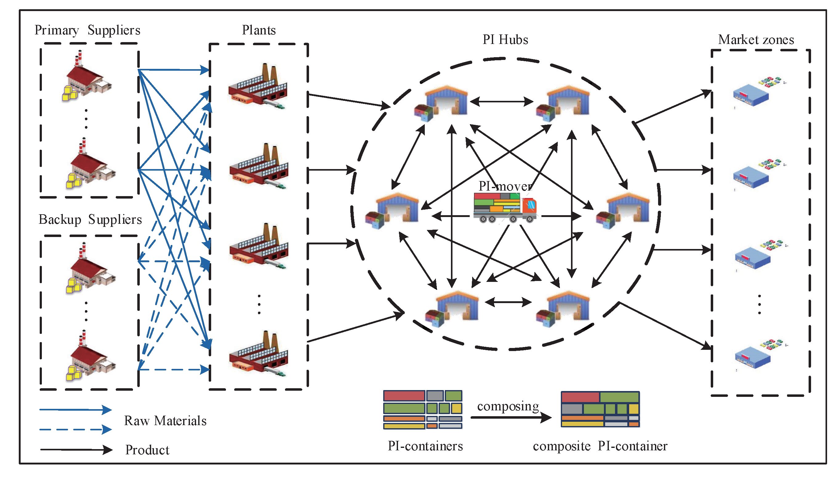
In this paper, we study an open supply network that consists of geographically dispersed plants and PI hubs. Each plant is served by several raw material suppliers that may differ from one another in terms of general, sustainable, and resilient performance. Raw materials flow from suppliers to plants, where they are transformed into final products and packed into standardized modular containers (PI containers). These containers can then be dynamically distributed to market zones through PI hubs, as illustrated in Figure 1.

Indeed, to optimize vehicle utilization, products can be processed, stored, and transported in the form of effective unit loads created by combined algorithms (i.e., composite PI containers). To transport the final products embedded in PI containers, a fleet of heterogeneous vehicles is available, denoted as $M=\{1,2,\dots ,|M\left|\right\}$. Transportation of products between nodes can be performed using transport vehicles $m\in M$ with varying weight capabilities. The deconsolidation and reconsolidation of PI containers into, within, and out of the PI hub are the core processes of PI-enabled multi-segment transportation. After processing at the PI hub, the reconsolidated PI containers can be shipped to the market zone or to another PI hub for further consolidation. After one or more PI hubs reconsolidate the product, the PI container is shipped to the market zone. Furthermore, vehicles may start their trips from one or more plants and return to the PI hub after completing deliveries in the market zones. After completing a delivery, the vehicle can return to the plant for replenishment. The PI containers are then reconsolidated at the PI hub and delivered to the market zone.

A complete graph, denoted as $G=(V^{\ast },A^{\ast })$, is constructed for the research problem in this paper. Here, $V^{\ast }$ represents a series of nodes consisting of a set of suppliers $V_s=V_p\cup V_b$, where $V_p$ and $V_b$ are primary and backup suppliers, respectively, and are defined as $V_p=\{1,2,\dots ,|V_p\left|\right\}$ and $V_b=\{1,2,\dots ,|V_b\left|\right\}$. In addition, $V^{\ast }$ also includes a set of plants $V_n=\{1,2,\dots ,,|V_n\left|\right\}$, a set of PI hubs $V_h=\{1,2,\dots ,|V_h\left|\right\}$, and a set of market zones $V_r=\{1,2,\dots ,|V_r\left|\right\}$. The set of arcs, denoted as $A^{\ast }=\{(i,j):i,j\in V^{\ast },i\ne j\}$, represents the connections between nodes, where each arc $(i,j)$ has a non-negative distance $d_{ij}$. The plant produces different types of products $k\in K=\{1,2,\dots ,|K\left|\right\}$ from raw materials or components supplied by selected qualified suppliers; each supplier $s\in V_s=\{1,2,\dots ,|V_s\left|\right\}$ offers the plant a limited supply capacity. The raw material suppliers, plants, and PI hubs are susceptible to disruption, in which a set of scenarios $\mathrm{\Omega }=\{1,2,\dots ,|\mathrm{\Omega }\left|\right\}$ is developed to indicate that one or more suppliers, plants, and PI hubs are impacted by the disruption. Moreover, since the likelihood of each facility (supplier, plant, or PI hub) being affected by multiple disruption events simultaneously is extremely low, this paper assumes that each facility may experience at most one disruption event in each scenario. Additionally, these facilities are geographically dispersed, meaning that a single disruption event will not affect all facilities simultaneously. In this paper, the following strategies are employed to improve the resilience of the supply chain: (1) allowing multiple backup procurement channels; (2) adding additional production capacity in the plant; and (3) the interconnection of PI hubs.

Of note, due to the unknown and unpredictable features of the market demand, fuzzy variables are suitable for realizing the market demand, avoiding the difficulty of obtaining demand distribution functions [97]. Additionally, cost parameters are difficult to determine as a function of changes in the international producer price index. In reality, raw materials may sustain damage during transportation from the supplier to the plant, resulting in an uncertain defect rate due to technical or human errors. Meanwhile, the supplier’s supply capacity and the plant’s production capacity after the disruption are uncertain. Thus, these input parameters are also fuzzy variables. Representing fuzzy variables with triangular fuzzy numbers is easier to implement, as it only requires estimating the maximum, minimum, and most probable values of the variables.

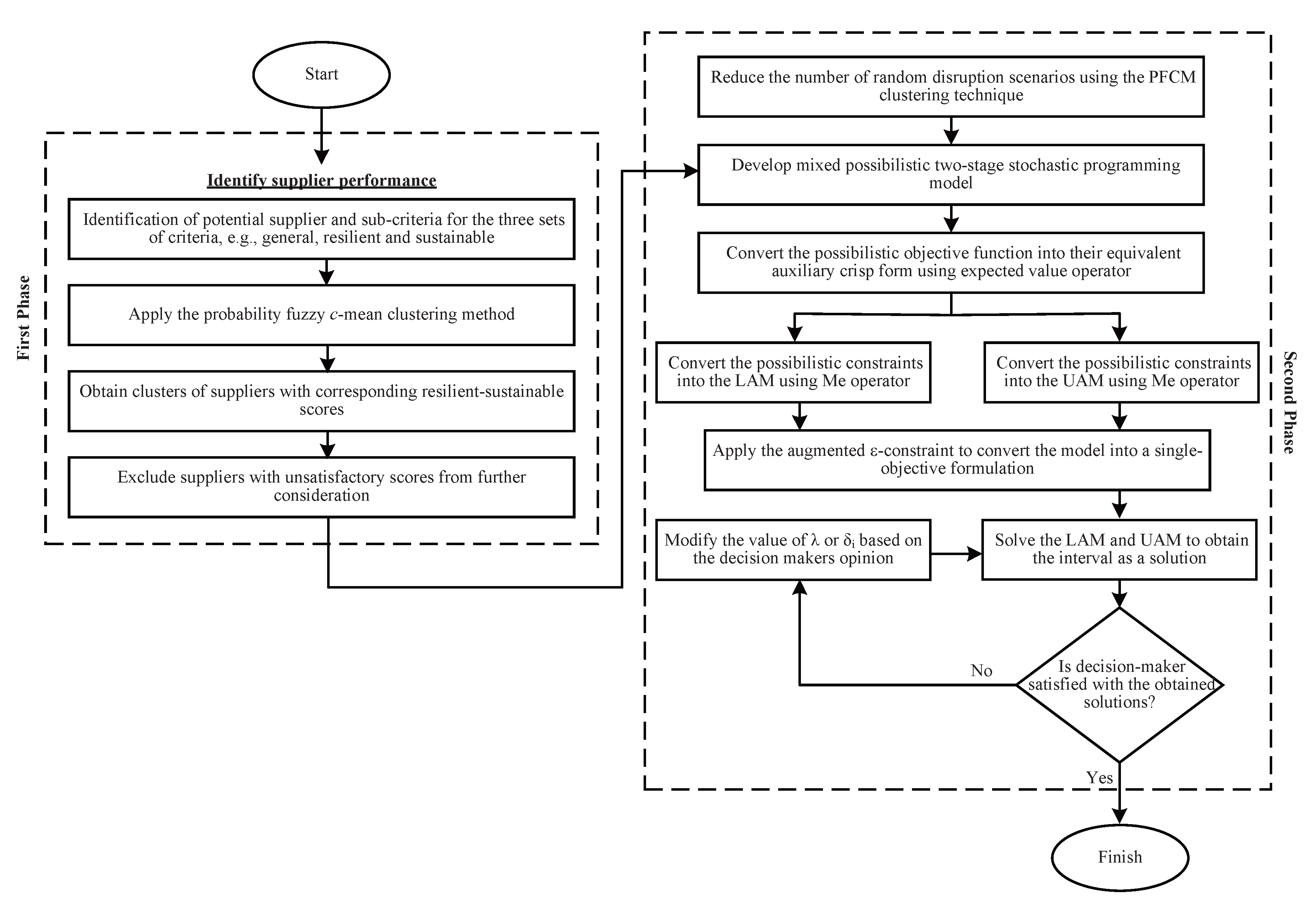
This paper employs a hybrid approach consisting of two stages to facilitate effective decision making. The first stage involves evaluating the resilient-sustainable performance of potential suppliers based on a variety of general, sustainable, and resilient indicators. The general, sustainable, and resilient indices were evaluated using the probability fuzzy c-means clustering method. Based on the resilient-sustainable performance scores, candidate suppliers were classified into different categories. The second stage involves using the resilient-sustainable performance score obtained in the first stage as an input parameter to establish a multi-objective mixed-possibilistic programming model that incorporates cost, sustainability, and resilience objectives. With different retailers holding different attitudes towards uncertainty, we use Me($\lambda$) to handle the objective function containing fuzzy variables. To obtain solutions that contain more information, we use rough set theory to deal with the feasible region that contains fuzzy variable constraints. On this basis, the scenario-based multi-objective mixed-possibilistic programming model is converted into two equivalent accurate models: the lower approximation model (LAM) and the upper approximation model (UAM). Finally, the Pareto solution is obtained using the augmented $\epsilon$-constraint method. Figure 2 shows the process framework of the two-stage approach. In the following sections, we will describe each stage in detail.

3.2. Supplier Resilient-Sustainable Performance Evaluation

When faced with supply disruptions, relying solely on cooperation with suppliers who excel in sustainable practices may limit flexibility in supplier switching. Therefore, it is of great practical significance to evaluate the supplier’s resilient-sustainable performance. The hybrid approach starts with the evaluation of the supplier’s resilient-sustainable performance. General performance criteria (e.g., cost, quality, delivery, technology capability, service, flexibility, financial, and trust [98]), sustainable performance criteria (e.g., green design capability, environmental management system, environmental competencies, pollution control, energy efficiency, eco-design recycling, green R&D and innovation, work safety/labor health, social management commitment, and the rights of people [99]), and resilient performance criteria (e.g., responsiveness, risk reduction, backup supplier contracting, geographical segregation, rerouting, cooperation, restorative capacity, and surplus inventory [84]) are employed. To evaluate the criteria, we invited industry experts to review the requirements based on previous studies in the literature [100,101]. A team of experts with at least five years of practical experience in the relevant field assessed the criteria. After evaluating supplier performance against each metric, we aggregated the results using the probabilistic fuzzy c-mean clustering method (PFCM) to classify suppliers into different clusters based on their resilient and sustainable performance scores. The overall resilient and sustainable performance of suppliers improves as their scores increase. Based on these scores, we identified and excluded suppliers with unsatisfactory resilient and sustainable performance, especially in the presence of supply disruptions.

Herewith, we describe the application framework of PFCM for clustering and evaluating suppliers’ resilient-sustainable performance. The PFCM was first introduced by [102], which was proposed to overcome the noise problem in the fuzzy c-mean method (FCM) and the overlapping clustering problem in the possibility c-mean method (PCM). Compared with FCM and PCM, PFCM provides a more informative data analysis. The PFCM provides the membership degree to confirm the data partition and the typical value of each point. It can be seen that the membership degree and the typical value are two indispensable measures. Based on the three outputs of PFCM, the supplier’s resilient-sustainable performance was evaluated: (1) the membership matrix represented by $u_{ij}$ used for fuzzy division; (2) the typical matrix in terms of $t_{ij}$ used to partition probabilities; (3) the set of model points $v_i$ used to represent cluster centers. Let us assume that to classify the n suppliers into c clusters. Furthermore, let ${\alpha }_j$ represent a vector of resilient-sustainable indicators reflecting supplier j performance. The steps are as follows:

Step 1.

Initialize iteration $L=1$, set threshold $\epsilon >0$, clustering numbers $c(1<c<n)$, $m,\eta \in [1,+\infty ]$ are the fuzzier constant, and the constants $a,b>0$. Let $u_{ij}\in [0,1]$ be the membership values of the supplier j belonging to cluster i, and $t_{ij}\in [0,1]$ be the typicality value of the supplier j belonging to cluster i.

Step 2.

Obtain the objective value of the PFCM clustering method as follows:

$$min{J}_L=\sum _{j=1}^n\sum _{i=1}^c(a{u_{ij}}^m+b{t_{ij}}^{\eta }){∥x_j-v_i∥}^2+\sum _{i=1}^c{\gamma }_i\sum _{j=1}^n{(1-t_{ij})}^{\eta }$$

(1)

where the parameters a and b in PFCM are used to indicate the influence of the membership value and typicality value, respectively. If $b>a$, the clustering center will be more influenced by the typicality value [102].

Step 3.

Compute the membership degrees for the current cluster center as follows:

$$u_{ij}={\left(\sum _{k=1}^c{\left(\frac{∥x_j-v_i∥}{∥x_j-v_k∥}\right)}^{2/\phantom{2m-1}m-1}\right)}^{-1}$$

(2)

Step 4.

Calculate the typical value of the current cluster center using the following equation:

$$t_{ij}={\left({\left(1+\frac{b∥x_j-v_i∥}{{\gamma }_i}\right)}^{2/\phantom{2\eta -1}\eta -1}\right)}^{-1}$$

(3)

Step 5.

Update the clustering centers as follows:

$$v_i=\frac{{\sum }_{j=1}^n\left(a{u}_{ij}^m+b{t}_{ij}^{\eta }\right)x_j}{{\sum }_{j=1}^n\left(a{u}_{ij}^m+b{t}_{ij}^{\eta }\right)}$$

(4)

Step 6.

If $∥J_L-J_{L-1}∥⩽\epsilon$, then go to Step 7; otherwise go to Step 2, $L=L+1$.

Step 7.

Exclude suppliers from clusters that are unsatisfactory in resilient-sustainable performance.

Step 8.

Considering both the membership degree and the typical value, the weight of supplier j belonging to cluster center i is as follows:

$$w_{ij}=u_{ij}{t}_{ij}$$

(5)

Step 9.

Return the resilient-sustainable score for the remaining suppliers by Equation (6):

$${\alpha }_j=\sum _{i=1}^c∥v_i∥w_{ij}$$

(6)

3.3. Mathematical Formulation

In the second phase, we developed an integrated multi-product PI-enabled supply–production–distribution model, and the supplier’s resilient-sustainable performance score was obtained in the first phase as input elements. A description of the defined model variables and parameters is shown in

Table 2. Notations of the model.

Sets and indices
$V_p$	Set of primary suppliers, denoted by index p
$V_b$	Set of backup suppliers, denoted by index b
Parameter
$V_n$	Set of plants, denoted by index n
$V_h$	Set of PI hubs, denoted by index h
$V_r$	Set of market zones, denoted by index r
V	Set of nodes, $V=V_n\cup V_h\cup V_r$
A	Set of arcs, $A=\left\{\right(i,j):i,j\in V,i\ne j\}$
L	Set of types of raw material, denoted by index l
K	Set of types of produces, denoted by index k
M	Set of vehicles, denoted by index m
$\mathrm{\Omega }$	Set of disruption scenarios, denoted by index $\xi$
Vehicle common parameter
$\epsilon$	Fuel-to-air mass ratio
g	Gravitational constant ($\mathrm{m}/\phantom{\mathrm{m}{\mathrm{s}}^2}{\mathrm{s}}^2$)
$\rho$	Air density ($\mathrm{kg}/\phantom{\mathrm{kg}{\mathrm{m}}^3}{\mathrm{m}}^3$)
$C_r$	Coefficient of rolling resistance
$\eta$	Efficiency parameter for diesel engines
$f_c$	Unit fuel cost (£/L)
$f_e$	Unit emission cost (£/kg)
$f_d$	Driver wage (£/s)
$\sigma$	Emitted by unit fuel consumption (kg/L)
k	Heating value of a typical diesel fuel (kj/g)
$vs.$	Speed (m/s)
$\psi$	Conversion factor (g/s to L/s)
$\theta$	Road angle
$\tau$	Acceleration ($\mathrm{m}/\phantom{\mathrm{m}{\mathrm{s}}^2}{\mathrm{s}}^2$)
Parameter
${\tilde{D}}_{ik\xi }$	Demand of product $k\in K$ at market zone $i\in V_r$ under scenario $\xi \in \mathrm{\Omega }$
$h_{lk}$	Quantity of raw material $l\in L$ required for production of a unit of product $k\in K$
${\alpha }_p$	Resilient-sustainable score of primary supplier $p\in V_p$ obtained from the pfcm
	clustering method
${\beta }_b$	Resilient-sustainable score of backup supplier $b\in V_b$ obtained from the pfcm
	clustering method
$C{P}_{pl}$	Initial supply capacity of raw material $l\in L$ by primary supplier $p\in V_p$
$S{C}_{bl}$	Initial supply capacity of raw material $l\in L$ by backup supplier $b\in V_b$
$\tilde{\delta }{}_{pl}$	Expected defect rate of raw material $l\in L$ primary supplier $p\in V_p$
$\tilde{\pi }{}_{bl}$	Expected defect rate of raw material $l\in L$ backup supplier $b\in V_b$
$\tilde{r}{}_{p\xi }$	Percentage supply capacity of primary supplier $p\in V_p$ disrupted under scenario $\xi \in \mathrm{\Omega }$
$L{T}_b$	Lead time of backup supplier $b\in V_b$
$\tilde{f}{}_p$	Fixed cost of evaluating and selecting primary supplier $p\in V_p$
$\tilde{s}{}_p$	Fixed setup cost of primary supplier $p\in V_p$
$\tilde{c}{}_b$	Fixed cost of contracting with backup supplier $b\in V_b$
$\widetilde{ps}{}_{pl}$	Unit cost of purchasing raw material $l\in L$ from primary supplier $p\in V_p$
$\widetilde{pr}{}_{bl}$	Unit cost of purchasing raw material $l\in L$ from backup supplier $b\in V_b$
$i{c}_{ik}$	Initial production capacity of product type $k\in K$ in plant $i\in V_n$
$e{c}_{ik}$	Maximum extendable capacity of product type $k\in K$ in plant $i\in V_n$
$\tilde{g}{}_{i\xi }$	Percentage production capacity of plant $i\in V_n$ disrupted under scenario $\xi \in \mathrm{\Omega }$
$\widetilde{pc}{}_{ik}$	Unit production cost of product type $k\in K$ in plant $i\in V_n$
$\tilde{e}{}_{ik}$	Unit cost of adding extra production capacity of product type $k\in K$ to plant $i\in V_n$
$L{T}_i$	Lead time of plant $i\in V_n$
$L{T_j}^{\prime }$	Lead time of PI hub $j\in V_h$
$\widetilde{hc}{}_{ik}$	Unit handling cost of product type $k\in K$ at node $i\in V$
$\tilde{b}{}_{ik}$	Unit lost sales cost of product type $k\in K$ in market zone $i\in V_r$
$d{}_{ij}$	Distance between node i and node j, $(i,j)\in A$
$p_{\xi }$	Possibility of occurrence of disruption scenario $\xi \in \mathrm{\Omega }$
$w{p}_k$	Weight of product type $k\in K$
$w_m$	Curb weight (kg)
$Q_m$	Maximum payload (kg)
$k_m$	Engine friction factor (kJ/rev/L)
$N_m$	Engine speed (rev/s)
$v_m$	Engine displacement (L)
$C_{dm}$	Coefficient of aerodynamics drag
$A_m$	Frontal surface area ($m^2$)
$n_m$	Vehicle drive train efficiency
Decision variables
$X_p$	If primary supplier $p\in V_p$ selected equals 1, otherwise 0
$X_b$	If backup supplier $b\in V_b$ selected equals 1, otherwise 0
$X_{ijm\xi }$	If arc $\left(i,j\right)$ visited by vehicle $m\in M$ under scenario $\xi \in \mathrm{\Omega }$ equals 1, otherwise 0
$E_{ik}$	Extra production capacity of product type $k\in K$ added to plant $i\in V_n$
Parameter
$U_{pil\xi }$	Quantity of raw material $l\in L$ picked up from primary supplier $p\in V_p$ to plant $i\in V_n$
	under scenario $\xi \in \mathrm{\Omega }$
$Y_{bil\xi }$	Quantity of raw material $l\in L$ picked up from backup supplier $b\in V_b$ to plant $i\in V_n$
	under scenario $\xi \in \mathrm{\Omega }$
$Z_{ik\xi }$	Quantity of product $k\in K$ production in the plant $i\in V_n$ under scenario $\xi \in \mathrm{\Omega }$
$p_{ikm\xi }$	Quantity of product $k\in K$ picked up from node $i\in V$ by vehicle $m\in M$ under scenario
	$\xi \in \mathrm{\Omega }$
$q_{ikm\xi }$	Quantity of product $k\in K$ delivered to node $i\in V$ by vehicle $m\in M$ under scenario
	$\xi \in \mathrm{\Omega }$
$V_{ijkm\xi }$	Quantity of product $k\in K$ by vehicle $m\in M$ between arc $\left(i,j\right)$ under scenario $\xi \in \mathrm{\Omega }$
$B_{ik\xi }$	Lost sales quantity of product type $k\in K$ at retail $i\in V_r$ under scenario $\xi \in \mathrm{\Omega }$

. Of note, each parameter with the symbol (~) represents an imprecise parameter, which can be expressed as a triangular fuzzy number.

3.3.1. Cost Objective

To estimate fuel consumption and emission costs, we apply the comprehensive model proposed by [103,104] to approximation calculate fuel consumption, which is further converted into emission costs. The fuel consumption $F_m\left(L\right)$ of a vehicle of type m with speed v for a distance d can be measured as follows: $F_m\left(L\right)=\lambda (k_m{N}_m{V}_m\left(d/\phantom{dv}v\right)+M_m{\gamma }_m\alpha d+{\beta }_m{\gamma }_{m}d{v}^2)$, in which $\lambda =\epsilon /\phantom{\epsilon \left(k\psi \right)}\left(k\psi \right)$, ${\gamma }_m=1/\phantom{1\left(1000n_m\eta \right)}\left(1000n_m\eta \right)$, $\alpha =\tau +\mathrm{gsin}\theta +\mathrm{g}{\mathrm{C}}_{\mathrm{r}}\cos \theta$, ${\beta }_m=0.5C_{dm}\rho A_m$, and $M_m$ for total vehicle weight (kg). The cost objective is proposed as follows:

$$\begin{array}{cc}\hfill f_1& ={\displaystyle \sum _{p\in V_p}}{X}_p\left(\tilde{s}{}_p+\tilde{f}{}_p\right)+\sum _{b\in V_b}{X}_b\tilde{c}{}_b+\sum _{\xi \in \mathrm{\Omega }}{p}_{\xi }\left(\sum _{l\in L}\sum _{p\in V_p}\sum _{i\in V_n}\frac{\widetilde{ps}{}_{pl}{U}_{pil\xi }}{1-\tilde{\delta }{}_{pl}}\right.\left.+\sum _{l\in L}\sum _{b\in V_b}\sum _{i\in V_n}\frac{\widetilde{pr}{}_{bl}{Y}_{bil\xi }}{1-\tilde{\pi }{}_{bl}}\right)\hfill \\ \hfill & +\sum _{\xi \in \mathrm{\Omega }}{p}_{\xi }\sum _{i\in V_n}\sum _{k\in K}\widetilde{pc}{}_{ik}{Z}_{ik\xi }+\sum _{k\in K}\sum _{i\in V_n}\tilde{e}{}_{ik}{E}_{ik}+\sum _{\xi \in \mathrm{\Omega }}{p}_{\xi }\sum _{i\in V}\sum _{k\in K}\sum _{m\in M}\widetilde{hc}{}_{ik}\left(p_{ikm\xi }+q_{ikm\xi }\right)\hfill \\ \hfill & +\sum _{\xi \in \mathrm{\Omega }}{p}_{\xi }\sum _{\left(i,j\right)\in A}\sum _{m\in M}\left(d_{ij}/\phantom{d_{ij}v}v\right)f_d{X}_{ijm\xi }+\sum _{\xi \in \mathrm{\Omega }}{p}_{\xi }\sum _{\left(i,j\right)\in A}\sum _{m\in M}\sum _{k\in K}\lambda \left[X_{ijm\xi }{k}_m{N}_m{V}_m\left(d_{ij}/\phantom{d_{ij}v}v\right)\right.\hfill \\ \hfill & +\left(w_m{X}_{ijm\xi }+\sum _{k\in K}w{p}_k{V}_{ijkm\xi }\right){\gamma }_m\alpha d_{ij}\left.+X_{ijm\xi }{\beta }_m{\gamma }_m{d}_{ij}{v}^2\right]\left(f_c+f_e\sigma \right)+\sum _{\xi \in \mathrm{\Omega }}{p}_{\xi }\sum _{i\in V_r}\sum _{k\in K}\tilde{b}{}_{ik}{B}_{ik\xi }\hfill \end{array}$$

(7)

The components of the cost function comprise the cost of evaluating and selecting the primary supplier, the cost of contracting with the backup supplier, the cost of procuring raw materials from primary and backup suppliers, the cost of plant production, the cost of adding additional production capacity, the cost incurred on loading and unloading, the cost of drivers’ wages, the cost of lost sales, the cost of fuel consumption and the cost of emissions for all vehicles at the PI-enabled supply network.

3.3.2. Sustainable Objective

Disruptions in supply chain activities are a significant obstacle to the development of sustainable supply chain networks. Thus, it is essential for the sustainable development of the supply chain that the supply chain is resilient and flexible sufficient to deal with supply disruptions. If the supplier is susceptible to disruptions, the plant will seek an alternative supplier to manage supply disruptions, regardless of its sustainability, to minimize the risks associated with disruptions. Hence, it is not comprehensive to use the supplier’s weighted sustainability score as the sole sustainable objective function in the presence of supply disruption risks. In this paper, the sustainable objective function is the total weighted resilient-sustainable scores of all suppliers under various disruption scenarios, as shown below:

$$f_2=\sum _{\xi \in \mathrm{\Omega }}{p}_{\xi }\left(\sum _{l\in L}\sum _{p\in V_p}\sum _{i\in V_n}\frac{{\alpha }_p{U}_{pil\xi }}{1-\tilde{\delta }{}_{pl}}+\sum _{l\in L}\sum _{b\in V_b}\sum _{i\in V_n}\frac{{\beta }_b{Y}_{bil\xi }}{1-\tilde{\pi }{}_{bl}}\right)$$

(8)

In particular, a sustainable objective that is more generic should incorporate the plant’s score for resilient and sustainable performance into Equation (8). Since our research is focused on analyzing and investigating supplier performance management in a PI-enabled supply chain, the objective function only takes into account the supplier’s weighted resilient and sustainable performance, while excluding the resilient and sustainable performance of plants from our research scope.

3.3.3. Resilience Objective

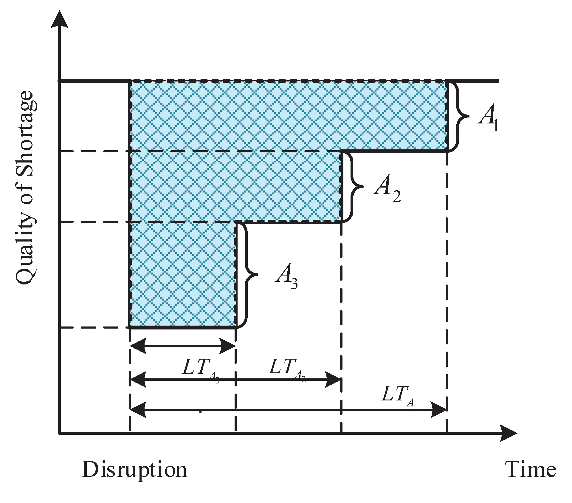
The resilience quantitative measurement method of disaster events proposed by [105] is nonlinear. Hence, Figure 3 illustrates the recovery process settings for disruptions occurring at suppliers, plants, and PI hubs in the PI-enabled supply–production–distribution problem presented in this paper.

In Figure 3, $A_1$, $A_2$, and $A_3$ indicate the number of products recovered from the disruption by the three resilience strategies of contracting with a backup supplier, adding additional capacity to the plant, and interconnecting PI hubs, respectively. $L{T}_{A_1}$, $L{T}_{A_2}$, and $L{T}_{A_3}$ denote the recovery time from the associated resilience strategy, respectively. It is observed that shaded areas indicate the resilience losses, calculated as $A_1\times L{T}_{A_1}+A_2\times L{T}_{A_2}+A_3\times L{T}_{A_3}$. RE calculates the number of products that are not received in the market zone without considering the resilience strategy. This calculation is used to determine the total resilience loss of the supply chain. Therefore, a new quantitative method is proposed to calculate the resilience loss of PI-enabled supply–production–distribution upon the occurrence of a random disruption, as follows:

$$RE=\sum _{\xi \in \mathrm{\Omega }}{p}_{\xi }\sum _{k\in K}\sum _{l\in L}\sum _{b\in V_b}\sum _{i\in V_n}L{T}_b{Y}_{bil\xi }/\phantom{L{T}_b{Y}_{bil\xi }{h}_{lk}}{h}_{lk}+\sum _{k\in K}\sum _{i\in V_n}L{T}_i{E}_{ik}+\sum _{\xi \in \mathrm{\Omega }}{p}_{\xi }\sum _{k\in K}\sum _{m\in M}\sum _{\left(i,j\right)\in V_h,i\ne j}L{T_j}^{\prime }{V}_{ijkm\xi }$$

(9)

The first item of Equation (9) represents the number of products produced from raw materials purchased from the backup suppliers multiplied by the time required to receive those products. The second term is the increased production capacity of the plant multiplied by the time to receive those products. Furthermore, the third item represents the number of products received by the PI hub from other PI hubs multiplied by the time required to receive these products from other PI hubs. RE is measured as the sum of the resilience recovery quantity multiplied by the corresponding delivery time. A lower value of RE indicates a smaller resilience loss in the supply network, indicating greater resilience in the network. In our problem, the vertical axis represents the total quantity of products required in the market zone. Therefore, the predicted resilience level of a PI-enabled supply chain can be determined. The resilience objective is measured using the following function:

$$f_3=1-\frac{RE}{Q·T^{\ast }}$$

(10)

where $Q={\displaystyle \sum _{i\in V_r}}{\displaystyle \sum _{k\in K}}{\displaystyle \sum _{\xi \in \mathrm{\Omega }}}\tilde{D}{}_{ik\xi }$ represents the total quantity of products required by the market zones, and $T^{\ast }$ indicates the maximum allowable time that the market zone is willing to wait for the recovery procedure.

3.3.4. Global Model

The global model is described below:

$$\begin{array}{cc}Min& f=\left(f_1,-f_2,-f_3\right)\end{array}$$

(11)

s.t.

$$\begin{array}{c}\sum _{i\in V_n}\frac{U_{pil\xi }}{1-\tilde{\mathrm{\delta }}{}_{pl}}⩽\left(1-\tilde{r}{}_{p\xi }\right)C{P}_{pl}{X}_p,\forall l\in L,\forall p\in V_p,\forall \xi \in \mathrm{\Omega }\end{array}$$

(12)

$$\begin{array}{c}\sum _{i\in V_n}\frac{Y_{bil\xi }}{1-\tilde{\pi }{}_{bl}}⩽C{P}_{bl}{X}_b,\forall l\in L,\forall b\in V_b,\forall \xi \in \mathrm{\Omega }\end{array}$$

(13)

$$\begin{array}{c}{Z}_{ik\xi }⩽\left(1-\tilde{g}{}_{i\xi }\right)\left(i{c}_{ik}+E_{ik}\right),\forall k\in K,\forall i\in V_n,\forall \xi \in \mathrm{\Omega }\end{array}$$

(14)

$$\begin{array}{c}{E}_{ik}⩽e{c}_{ik},\forall k\in K,\forall i\in V_n\end{array}$$

(15)

$$\begin{array}{c}\sum _{p\in V_p}\frac{U_{pil\xi }}{1-\tilde{\delta }{}_{pl}}+\sum _{b\in V_b}\frac{Y_{bil\xi }}{1-\tilde{\pi }{}_{bl}}=\sum _{k\in K}{Z}_{ik\xi }{h}_{lk},\forall l\in L,\forall i\in V_n,\forall \xi \in \mathrm{\Omega }\end{array}$$

(16)

$$\begin{array}{c}{Z}_{ik\xi }=\sum _{m\in M}{p}_{ikm\xi },\forall k\in K,\forall i\in V_n,\forall \xi \in \mathrm{\Omega }\end{array}$$

(17)

$$\begin{array}{c}\sum _{m\in M}{p}_{ikm\xi }=\sum _{m\in M}{q}_{ikm\xi },\forall k\in K,\forall i\in V_h,\forall \xi \in \mathrm{\Omega }\end{array}$$

(18)

$$\begin{array}{c}\sum _{m\in M}{q}_{ikm\xi }+B_{ik\xi }=\tilde{D}{}_{ik\xi },\forall i\in V_r,\forall k\in K,\forall \xi \in \mathrm{\Omega }\end{array}$$

(19)

$$\begin{array}{c}{q}_{ikm\xi }=0,\forall k\in K,\forall i\in V_n,\forall m\in M,\forall \xi \in \mathrm{\Omega }\end{array}$$

(20)

$$\begin{array}{c}{p}_{ikm\xi }=0,\forall k\in K,\forall i\in V_r,\forall m\in M,\forall \xi \in \mathrm{\Omega }\end{array}$$

(21)

$$\begin{array}{c}\sum _{i\in V}{X}_{ijm\xi }=\sum _{i\in V}{X}_{jim\xi },\forall j\in V,i\ne j,\forall m\in M,\forall \xi \in \mathrm{\Omega }\end{array}$$

(22)

$$\begin{array}{c}\sum _{j\in V}{X}_{ijm\xi }⩽1,\forall i\in V,i\ne j,\forall m\in M,\forall \xi \in \mathrm{\Omega }\end{array}$$

(23)

$$\begin{array}{c}\sum _{i\in V}\sum _{m\in M}{X}_{ijm\xi }⩽1,\forall j\in V,i\ne j,\forall \xi \in \mathrm{\Omega }\end{array}$$

(24)

$$\begin{array}{c}\sum _{k\in K}{V}_{ijkm\xi }⩽Q_m{X}_{ijm\xi },\forall \left(i,j\right)\in V,i\ne j,\forall m\in M,\forall \xi \in \mathrm{\Omega }\end{array}$$

(25)

$$\begin{array}{c}\sum _{j\in V}{V}_{ijkm\xi }-\sum _{j\in V}{V}_{jikm\xi }=q_{ikm\xi }-p_{ikm\xi },\forall i\in V,i\ne j,\forall k\in K,\forall m\in M,\forall \xi \in \mathrm{\Omega }\end{array}$$

(26)

$$\begin{array}{ccccc}\hfill & \hfill & \hfill \sum _{i\in V}{X}_{iim\xi }& =0,\forall i\in V,\forall m\in M,\forall \xi \in \mathrm{\Omega }\hfill & \end{array}$$

(27)

$$\begin{array}{cccccc}\hfill & \hfill & \hfill X_{ijm\xi }& =0,\forall i\in V_p\cup V_b,\forall j\in V_h,\forall m\in M,\forall \xi \in \mathrm{\Omega }\hfill & \hfill & \end{array}$$

(28)

$$\begin{array}{ccccc}\hfill & \hfill & \hfill X_{ijm\xi }& =0,\forall i\in V_p\cup V_b,\forall j\in V_r,\forall m\in M,\forall \xi \in \mathrm{\Omega }\hfill & \end{array}$$

(29)

$$\begin{array}{ccccc}\hfill & \hfill & \hfill X_{ijm\xi }& =0,\forall i\in V_n,\forall j\in V_p\cup V_b,\forall m\in M,\forall \xi \in \mathrm{\Omega }\hfill & \end{array}$$

(30)

$$\begin{array}{ccccc}\hfill & \hfill & \hfill X_p& \in \left\{0,1\right\},\forall p\in V_p\hfill & \end{array}$$

(31)

$$\begin{array}{ccccc}\hfill & \hfill & \hfill X_b& \in \left\{0,1\right\},\forall b\in V_b\hfill & \end{array}$$

(32)

$$\begin{array}{ccccc}\hfill & \hfill & \hfill X_{ijm\xi }& \in \left\{0,1\right\},\forall i,j\in V,i\ne j,\forall m\in M,\forall \xi \in \mathrm{\Omega }\hfill & \end{array}$$

(33)

$$\begin{array}{ccccc}\hfill & \hfill & \hfill E_{ik}& \in Z^{\ast },\forall k\in K,\forall n\in V_n\hfill & \end{array}$$

(34)

$$\begin{array}{ccccc}\hfill & \hfill & \hfill U_{pil\xi }& \in Z^{\ast },\forall l\in L,\forall p\in V_p,,\forall i\in V_n,\forall \xi \in \mathrm{\Omega }\hfill & \end{array}$$

(35)

$$\begin{array}{ccccc}\hfill & \hfill & \hfill Y_{bil\xi }& \in Z^{\ast },\forall l\in L,\forall b\in V_b,\forall i\in V_n,\forall \xi \in \mathrm{\Omega }\hfill & \end{array}$$

(36)

$$\begin{array}{ccccc}\hfill & \hfill & \hfill Z_{ik\xi }& \in Z^{\ast },\forall i\in V_n,\forall k\in K,\forall \xi \in \mathrm{\Omega }\hfill & \end{array}$$

(37)

$$\begin{array}{ccccc}\hfill & \hfill & \hfill p_{ikm\xi }& \in Z^{\ast },\forall i\in V,\forall k\in K,\forall m\in M,\forall \xi \in \mathrm{\Omega }\hfill & \end{array}$$

(38)

$$\begin{array}{ccccc}\hfill & \hfill & \hfill q_{ikm\xi }& \in Z^{\ast },\forall i\in V,\forall k\in K,\forall m\in M,\forall \xi \in \mathrm{\Omega }\hfill & \end{array}$$

(39)

$$\begin{array}{ccccc}\hfill & \hfill & \hfill V_{ijkm\xi }& \in Z^{\ast },\forall k\in K,\forall i,j\in V,i\ne j,\forall \xi \in \mathrm{\Omega }\hfill & \end{array}$$

(40)

$$\begin{array}{cccc}\hfill & \hfill & \hfill B_{ik\xi }& \in Z^{\ast },\forall k\in K,\forall i\in V_r,\forall \xi \in \mathrm{\Omega }\hfill \end{array}$$

(41)

Constraints (12) and (13) restrict the capacity of the primary suppliers and backup suppliers, respectively. Constraints (14) and (15) guarantee the capacity limitations of the plants. Constraint (16) ensures that the raw material requirements of the plant are met. Constraints (17)–(19) indicate the flow balance restrictions for the plants, PI hubs, and market zones, respectively. Constraints (20) and (21) represent that delivery of the PI container to the plant and pick-up from the market zone are not permitted, respectively. Constraint (22) guarantees that the vehicle must leave at the end of its visit to a node. Constraints (23) and (24) address that each vehicle can only implement one route in each scenario. Constraint (25) indicates that the sum of the transportation quantities of all products in a certain transportation route does not exceed the maximum load of the vehicle. Constraint (26) measures the weight level of each product transported by the vehicle along its route. Constraint (27) ensures that product transport does not exist between identical nodes. Constraints (28) and (29) indicate that it is not permissible to transport raw materials from suppliers to PI hubs and market zones, respectively. Constraint (30) indicates that in each scenario, the plant is not allowed to supply the supplier. Finally, constraints (31)–(41) determine the domains of the variables.

4. Solution Method

In this paper, we apply a hybrid interactive solution method to solve the model, where the decision maker and model analyzer work together to obtain an optimal compromise solution. The details of the solution process are presented in Section 4.1, Section 4.2, and Section 4.3, respectively.

4.1. Scenario Reduction Procedure

To account for disruption uncertainty, a set of potential disruption scenarios is designed to represent one or more suppliers, plants, and PI hubs that may be affected by the disruption. It is evident that the number of disruption scenarios increases exponentially as the number of disruption events and supply chain participants (suppliers, plants, and PI hubs) increases. This results in models that become too large to be effectively solved. For example, if the number of suppliers, plants, and PI hubs is five, and each supply chain participant has 20 different disruption events, then the total number of disruption event scenarios is ${\left(20+1\right)}^{15}$. In reality, it is cumbersome or even impossible to consider all disruption events to solve the problem. Therefore, this paper applies the PFCM algorithm for scenario reduction to reduce the difficulty of model solving. The scenario reduction procedure applied in this paper is divided into two steps.

In the first step, the number of disruption scenarios in the model designed in this paper grows exponentially with the number of disruption events. To decrease the number of disruption event scenarios, PFCM is utilized to cluster the possible disruption events of each supply chain participant into various clusters. The center of each cluster serves as a representative of the disruption events. In this process, the probability of disruption event occurrence is used as the primary feature in the clustering process. The first step reduces the number of disruption events for each supply chain participant from 20 to 3, which greatly reduces the computation. Nevertheless, the number of disruption scenarios increases exponentially with the number of supply chain participants (suppliers, plants, and PI hubs), resulting in a vast number of scenarios due to the significant number of supply chain participants involved. For example, when the number of suppliers, plants, and PI hubs are 5, and the number of disruption events for each supply chain participant is 1, the total number of disruption scenarios is $2^5\times 2^5\times 2^5$. Therefore, it is not possible to consider all potential disruption scenarios. In the second step, the PFCM algorithm is applied to cluster the possible disruption scenarios into distinct clusters based on their disruption scale, which may be small, medium, or large. The center of each cluster is considered a representation of the corresponding disruption scale. Among them, the number of disruptions of suppliers, plants, and PI hubs is regarded as the main characteristics of the clustering process. In this paper, we apply the above two steps to reduce the number of disruption scenarios. Additionally, since disruption events occur independently, each disruption scenario is associated with a given number of undisrupted and disrupted supply chain participants (suppliers, plants, and PI hubs), and each disrupted supply chain participant faces one specific disruptive event. Therefore, the likelihood of the scenario can be calculated as follows:

$$P_{\xi }={\displaystyle \sum _{s\in S}}\left[{\displaystyle \prod _{i\in W_{\xi }}}{\pi }_{is}{\displaystyle \prod _{i\in \overline{W_{\xi }}}}\left(1-{\pi }_{is}\right)\right]$$

where ${\pi }_{is}$ is the probability of disruption event s occurring in supply chain participant i, $W_{\xi }$ is the supply chain participant who is disrupted in the disruption scenario $\xi$, and $\overline{W_{\xi }}$ is the undisrupted supply chain participant in the disruption scenario $\xi$.

4.2. The Equivalent Aided Crisp Model

In our model, to deal with the uncertainty of the input data, we adopt the mixed-possibilistic programming method based on the fuzzy measure Me introduced by [106] to convert the proposed model into an equivalent auxiliary crisp model. Compared with other fuzzy measures, Me-based measures can avoid extreme attitudes and reduce information loss. That is, Me-based measurement combines the two standard fuzzy measures of probability (Pos) and necessity (Nec), which can represent any attitude between extreme optimism and extreme pessimism. It is noteworthy that the feasible solution region of UAM is greater than that of LAM due to the optimistic attitude held by UAM and the pessimistic attitude held by LAM in the constraint. Consequently, the solution interval is derived by solving the LAM and UAM models, where the output of UAM represents the upper bound, and the output of LAM represents the lower bound. Through these two models, decision makers will obtain the best decision interval to obtain more information, which is helpful for the final solution selection [106].

4.2.1. Handling Fuzzy Objectives

By considering $\mathrm{\Lambda }=\left(\mathrm{\Theta },P\left(\mathrm{\Theta }\right),Pos\right)$ as a possibility space, the Me-based expected value is defined as follows [106]:

$$Me\left\{A\right\}=Nec\left\{A\right\}+\lambda \left(Pos\left\{A\right\}-Nec\left\{A\right\}\right)$$

(42)

where $\lambda$ is the parameter by which decision makers adjust their attitudes between absolute optimism and absolute pessimism. Given a fuzzy variable $\zeta$, the expected value defined Me($\lambda$)-based is as follows:

$$E\left[\zeta \right]={\int }_0^{+\infty }Me\left\{\zeta ⩾r\right\}dr-{\int }_{-\infty }^{0}Me\left\{\zeta ⩽r\right\}dr$$

(43)

According to the definition of the Me-based fuzzy measure, we can calculate the expected value of the objective functions and take them as the objective function of the equivalent crisp model. If the fuzzy variable $\widetilde{s_p}$ is considered as the triangular fuzzy number $\widetilde{s_p}=\left({\alpha }_p^s,s_p,{\beta }_p^s\right)$, where ${\alpha }_p^s$ and ${\beta }_p^s$ are the lower and upper bounds of the fuzzy number, respectively, and $s_p$ is the most probable value. The objective function of our proposed model using the Me measure is reported in Appendix A.

4.2.2. Handling Fuzzy Constraints

To reduce information loss, rough set theory is used to divide the fuzzy feasible regions when converting the mixed-possibilistic programming model into a crisp model. Using rough approximation to handle fuzzy constraints, two approximate models are obtained that demonstrate the various perspectives of decision makers toward fuzzy constraints. The feasible region of the upper approximation model (UAM) indicates that the decision maker has an optimistic view of the fuzzy constraint, while the feasible region of the lower approximation model (LAM) indicates that the decision maker has a pessimistic view of the fuzzy constraint [106]. Therefore, the constraints of UAM are represented by

$$\begin{array}{c}\hfill \left\{\begin{array}{c}{\displaystyle \sum _{i\in V_n}}\frac{U_{pil\xi }}{1-\left({\delta }_{pl}-\left(1-{\delta }_1\right){\beta }_{pl}^{\delta }\right)}⩽\left(1-\left(r_{p\xi }+\left(1-{\delta }_1\right){\beta }_{p\xi }^r\right)\right)C{P}_{pl}{X}_p,\forall l\in L,\forall p\in V_p,\forall \xi \in \mathrm{\Omega }\hfill \\ {\displaystyle \sum _{i\in V_n}}\frac{Y_{bil\xi }}{1-\left({\pi }_{bl}-\left(1-{\delta }_2\right){\beta }_{bl}^{\pi }\right)}⩽C{P}_{bl}{X}_b,\forall l\in L,\forall b\in V_b,\forall \xi \in \mathrm{\Omega }\hfill \\ Z_{ik\xi }⩽\left(1-\left(g_{i\xi }+\left(1-{\delta }_3\right){\beta }_{i\xi }^g\right)\right)\left(i{c}_{ik}+E_{ik}\right),\forall k\in K,\forall i\in V_n,\forall \xi \in \mathrm{\Omega }\hfill \\ {\displaystyle \sum _{p\in V_p}}\frac{U_{pil\xi }}{1-\left({\delta }_{pl}-\left(1-{\delta }_4\right){\beta }_{pl}^{\delta }\right)}+{\displaystyle \sum _{b\in V_b}}\frac{Y_{bil\xi }}{1-\left({\pi }_{bl}-\left(1-{\delta }_4\right){\beta }_{bl}^{\pi }\right)}={\displaystyle \sum _{k\in K}}{Z}_{ik\xi }{h}_{lk}\hfill \\ ,\forall l\in L,\forall i\in V_n,\forall \xi \in \mathrm{\Omega }\hfill \\ {\displaystyle \sum _{m\in M}}{q}_{ikm\xi }+B_{ik\xi }=D_{ik\xi }+\left(1-{\delta }_5\right){\beta }_{ik\xi }^D,\forall i\in V_r,\forall k\in K,\forall \xi \in \mathrm{\Omega }\hfill \end{array}\right.\end{array}$$

(44)

and $v\in F\left(vs.\right)$, where v is the feasible solution containing all variables. Also, $F\left(vs.\right)$ stands for the feasible domain (15), (17), (18), and (20)–(41) that do not contain fuzzy constraints. The constraints of LAM are represented by

$$\begin{array}{c}\hfill \left\{\begin{array}{c}{\displaystyle \sum _{i\in V_n}}\frac{U_{pil\xi }}{1-\left({\delta }_{pl}+\left(1-{\delta }_6\right){\beta }_{pl}^{\delta }\right)}⩽\left(1-\left(r_{p\xi }-\left(1-{\delta }_6\right){\beta }_{p\xi }^r\right)\right)C{P}_{pl}{X}_p,\forall l\in L,\forall p\in V_p,\forall \xi \in \mathrm{\Omega }\hfill \\ {\displaystyle \sum _{i\in V_n}}\frac{Y_{bil\xi }}{1-\left({\pi }_{bl}+\left(1-{\delta }_7\right){\beta }_{bl}^{\pi }\right)}⩽C{P}_{bl}{X}_b,\forall l\in L,\forall b\in V_b,\forall \xi \in \mathrm{\Omega }\hfill \\ Z_{ik\xi }⩽\left(1-\left(g_{i\xi }-\left(1-{\delta }_8\right){\beta }_{i\xi }^g\right)\right)\left(i{c}_{ik}+E_{ik}\right),\forall k\in K,\forall i\in V_n,\forall \xi \in \mathrm{\Omega }\hfill \\ {\displaystyle \sum _{p\in V_p}}\frac{U_{pil\xi }}{1-\left({\delta }_{pl}+\left(1-{\delta }_9\right){\beta }_{pl}^{\delta }\right)}+{\displaystyle \sum _{b\in V_b}}\frac{Y_{bil\xi }}{1-\left({\pi }_{bl}+\left(1-{\delta }_9\right){\beta }_{bl}^{\pi }\right)}={\displaystyle \sum _{k\in K}}{Z}_{ik\xi }{h}_{lk}\hfill \\ ,\forall l\in L,\forall i\in V_n,\forall \xi \in \mathrm{\Omega }\hfill \\ {\displaystyle \sum _{m\in M}}{q}_{ikm\xi }+B_{ik\xi }=D_{ik\xi }-\left(1-{\delta }_{10}\right){\beta }_{ik\xi }^D,\forall i\in V_r,\forall k\in K,\forall \xi \in \mathrm{\Omega }\hfill \end{array}\right.\end{array}$$

(45)

and $v\in F\left(vs.\right)$.

4.2.3. The Development of Crisp Equivalent Global Model

As mentioned above, the two equivalent crisp models are reported as follows. UAM is expressed as

$$\left\{\begin{array}{c}\begin{array}{cc}Min& E^{Me}\left[\tilde{f}{}_1\right]\end{array}\hfill \\ \begin{array}{cc}Max& E^{Me}\left[\tilde{f}{}_2\right]\end{array}\hfill \\ \begin{array}{cc}Max& E^{Me}\left[\tilde{f}{}_3\right]\end{array}\hfill \\ s.t.\left\{\begin{array}{c}{\displaystyle \sum _{i\in V_n}}\frac{U_{pil\xi }}{1-\left({\delta }_{pl}-\left(1-{\delta }_1\right){\beta }_{pl}^{\delta }\right)}⩽\left(1-\left(r_{p\xi }+\left(1-{\delta }_1\right){\beta }_{p\xi }^r\right)\right)C{P}_{pl}{X}_p\hfill \\ ,\forall l\in L,\forall p\in V_p,\forall \xi \in \mathrm{\Omega }\hfill \\ {\displaystyle \sum _{i\in V_n}}\frac{Y_{bil\xi }}{1-\left({\pi }_{bl}-\left(1-{\delta }_2\right){\beta }_{bl}^{\pi }\right)}⩽C{P}_{bl}{X}_b,\forall l\in L,\forall b\in V_b,\forall \xi \in \mathrm{\Omega }\hfill \\ Z_{ik\xi }⩽\left(1-\left(g_{i\xi }+\left(1-{\delta }_3\right){\beta }_{i\xi }^g\right)\right)\left(i{c}_{ik}+E_{ik}\right),\forall k\in K,\forall i\in V_n,\forall \xi \in \mathrm{\Omega }\hfill \\ {\displaystyle \sum _{p\in V_p}}\frac{U_{pil\xi }}{1-\left({\delta }_{pl}-\left(1-{\delta }_4\right){\beta }_{pl}^{\delta }\right)}+{\displaystyle \sum _{b\in V_b}}\frac{Y_{bil\xi }}{1-\left({\pi }_{bl}-\left(1-{\delta }_4\right){\beta }_{bl}^{\pi }\right)}={\displaystyle \sum _{k\in K}}{Z}_{ik\xi }{h}_{lk}\hfill \\ ,\forall l\in L,\forall i\in V_n,\forall \xi \in \mathrm{\Omega }\hfill \\ {\displaystyle \sum _{m\in M}}{q}_{ikm\xi }+B_{ik\xi }=D_{ik\xi }+\left(1-{\delta }_5\right){\beta }_{ik\xi }^D,\forall i\in V_r,\forall k\in K,\forall \xi \in \mathrm{\Omega }\hfill \\ v\in F\left(vs.\right)\hfill \end{array}\right.\hfill \end{array}\right.$$

(46)

Furthermore, LAM is represented as

$$\left\{\begin{array}{c}\begin{array}{cc}Min& E^{Me}\left[\tilde{f}{}_1\right]\end{array}\hfill \\ \begin{array}{cc}Max& E^{Me}\left[\tilde{f}{}_2\right]\end{array}\hfill \\ \begin{array}{cc}Max& E^{Me}\left[\tilde{f}{}_3\right]\end{array}\hfill \\ s.t.\left\{\begin{array}{c}{\displaystyle \sum _{i\in V_n}}\frac{U_{pil\xi }}{1-\left({\delta }_{pl}+\left(1-{\delta }_6\right){\beta }_{pl}^{\delta }\right)}⩽\left(1-\left(r_{p\xi }-\left(1-{\delta }_6\right){\beta }_{p\xi }^r\right)\right)C{P}_{pl}{X}_p\hfill \\ ,\forall l\in L,\forall p\in V_p,\forall \xi \in \mathrm{\Omega }\hfill \\ {\displaystyle \sum _{i\in V_n}}\frac{Y_{bil\xi }}{1-\left({\pi }_{bl}+\left(1-{\delta }_7\right){\beta }_{bl}^{\pi }\right)}⩽C{P}_{bl}{X}_b,\forall l\in L,\forall b\in V_b,\forall \xi \in \mathrm{\Omega }\hfill \\ Z_{ik\xi }⩽\left(1-\left(g_{i\xi }-\left(1-{\delta }_8\right){\beta }_{n\xi }^g\right)\right)\left(i{c}_{ik}+E_{ik}\right),\forall k\in K,\forall i\in V_n,\forall \xi \in \mathrm{\Omega }\hfill \\ {\displaystyle \sum _{p\in V_p}}\frac{U_{pil\xi }}{1-\left({\delta }_{pl}+\left(1-{\delta }_9\right){\beta }_{pl}^{\delta }\right)}+{\displaystyle \sum _{b\in V_b}}\frac{Y_{bil\xi }}{1-\left({\pi }_{bl}+\left(1-{\delta }_9\right){\beta }_{bl}^{\pi }\right)}={\displaystyle \sum _{k\in K}}{Z}_{ik\xi }{h}_{lk}\hfill \\ ,\forall l\in L,\forall i\in V_n,\forall \xi \in \mathrm{\Omega }\hfill \\ {\displaystyle \sum _{m\in M}}{q}_{ikm\xi }+B_{ik\xi }=D_{ik\xi }-\left(1-{\delta }_{10}\right){\beta }_{ik\xi }^D,\forall i\in V_r,\forall k\in K,\forall \xi \in \mathrm{\Omega }\hfill \\ v\in F\left(vs.\right)\hfill \end{array}\right.\hfill \end{array}\right.$$

(47)

4.3. The Augmented $\epsilon$-Constraint Method

The two equivalent auxiliary crisp models presented in Section 4.2 are multi-objective models. The augmented $\epsilon$-constraint algorithm proposed by [107] is used to ensure that the solutions produced by UAM and LAM are valid. Assuming that the cost objective gets priority followed by the sustainable and resilience objective, respectively, we convert the objective functions $f_2$ and $f_3$ into constraints ${\epsilon }_{sus}$ and ${\epsilon }_{res}$. This method can find effective solutions to the problems presented in this paper. To describe the augmented $\epsilon$-constraint method for our problem, the process is shown in Algorithm 1.

Algorithm 1: Pseudo-code of the augmented $\epsilon$-constraint method.

5. Computational Experiments

In this section, we describe the implementation of the constructed model. We consider two plants that require raw materials, which are purchased from three pre-qualified primary suppliers and two backup suppliers. The production process is identical across both plants, and plant capacity can be increased through the addition of fixed equipment. Two different products are shipped from the plant to four PI hubs to serve five market zones. PI containers are transported using three types of heterogeneous vehicles, each of which has a load of 10 tons and travels at a fixed speed of 80 km/h. Fuel prices, unit greenhouse gas emissions cost, and driver wages are 0.7382 (RMB/L), 0.248 (RMB/L), and 0.0022 (RMB/L), respectively, [108,109,110]. The fuel conversion coefficient and road angular surface line are 2.63 kg/L and 0 [111], respectively. The product has a weight of 100 kg per container. This paper generated imprecise and precise parameters using uniform distributions. Each imprecise parameter was modeled with a suitable probability distribution in the form of a symmetric triangular fuzzy number, where the symmetric distribution is 20% of the central value. The other problem parameters in the numerical experiments are shown in

Table 3. Range of uniform distributions used to generate the center of symmetric fuzzy parameters.

Parameter	Range of Uniform Distribution	Parameter	Range of Uniform Distribution
$\tilde{D}{}_{jk\xi }$	$50\times U\left[1.0,5.0\right]$	$\widetilde{ps}{}_{pl}$	$U\left[0.5,2.5\right]$
$\tilde{\delta }{}_{pl}$	$U\left[0.01,0.10\right]$	$\widetilde{pr}{}_{bl}$	$\tilde{p}{}_{pl}+U\left[1.0,3.0\right]$
$\tilde{\pi }{}_{bl}$	$U\left[0.05,0.15\right]$	$\tilde{g}{}_{i\xi }$	$U\left[0.1,0.4\right]$
$\tilde{r}{}_{p\xi }$	$U\left[0.2,0.6\right]$	$\widetilde{pc}{}_{ik}$	$U\left[2.0,10.0\right]$
$\tilde{f}{}_p$	$25\times U\left[4,10\right]$	$\tilde{e}{}_{ik}$	$\widetilde{pc}{}_{ik}+U\left[2.0,5.0\right]$
$\tilde{s}{}_p$	$U\left[11.0,15.0\right]$	$\widetilde{hc}{}_{ik}$	$0.15\times \left(\widetilde{pc}{}_{ik}/\phantom{\widetilde{pc}{}_{ik}3}3\right)$
$\tilde{c}{}_b$	$30\times U\left[4,10\right]$	$\tilde{b}{}_{ik}$	$U\left[25.0,50.0\right]$

and

Table 4. Range of uniform distributions used to generate crisp parameters.

Parameter	Range of Uniform Distribution	Parameter	Range of Uniform Distribution
$h_{lk}$	$U\left[30,40\right]$	$e{c}_{ik}$	$U\left[11.0,12.0\right]$
$C{P}_{pl}$	$U\left[400,1000\right]$	$L{T}_i$	$L{T}_j^{\prime }+U\left[5,15\right]$
$S{C}_{bl}$	$U\left[200,1000\right]$	$L{T_j}^{\prime }$	$U\left[35,55\right]$
$L{T}_b$	$U\left[30,50\right]$	$d_{ij}$	$U\left[100,500\right]$
$i{c}_{ik}$	$U\left[400,1000\right]$	$w_m$	$U\left[4000,20,000\right]$
$Q_m$	$U\left[2000,20,000\right]$	$C_{dm}$	$U\left[0.5,1.0\right]$
$k_m$	$U\left[0.1,0.3\right]$	$A_m$	$U\left[9.0,10.0\right]$
$N_m$	$U\left[30,40\right]$	$n_m$	$U\left[0.40,0.50\right]$
$v_m$	$U\left[2.0,7.0\right]$	$T^{\ast }$	100

.

The first step of the proposed solution methodology involves establishing a resilient-sustainable assessment measure. This is achieved by forming a team of experts who visit each supplier. PFCM was applied to measure performance across three dimensions: general (cost, service, and flexibility), sustainable (green design capabilities, environmental management systems, and social management organizations), and resilient (responsiveness, geographical segregation, and collaboration). The elements in PFCM are set to $a=2$, $b=5$, $m=2$, $\eta =2$, maxiter = 1000, and the number cluster $c=3$. The supplier’s resilient-sustainable performance evaluation is run in MATLAB R2018a, and the relevant data are reported in Appendix B (

Table A1. Performance assessment of suppliers.

Supplier	General Criteria			Sustainable Criteria			Resilient Criteria
	${\mathbf{C}}_{\mathbf{1}}$	${\mathbf{C}}_{\mathbf{2}}$	${\mathbf{C}}_{\mathbf{3}}$	${\mathbf{C}}_{\mathbf{4}}$	${\mathbf{C}}_{\mathbf{5}}$	${\mathbf{C}}_{\mathbf{6}}$	${\mathbf{C}}_{\mathbf{7}}$	${\mathbf{C}}_{\mathbf{8}}$	${\mathbf{C}}_{\mathbf{9}}$
$S_1$	0.4	0.6	0.3	0.1	0.3	0.6	0.6	0.4	0.2
$S_2$	0.8	0.6	0.1	0.4	0.6	0.5	0.4	0.1	0.3
$S_3$	0.6	0.8	0.5	0.1	0.5	0.2	0.2	0.7	0.4
$S_4$	0.1	0.5	0.4	0.7	0.5	0.6	0.5	0.1	0.5
$S_5$	0.5	0.1	0.4	0.6	0.5	0.4	0.1	0.5	0.6
$S_6$	0.2	0.4	0.5	0.2	0.1	0.6	0.8	0.4	0.3
$S_7$	0.4	0.5	0.1	0.5	0.7	0.5	0.5	0.6	0.3
$S_8$	0.6	0.1	0.5	0.5	0.6	0.6	0.7	0.2	0.5
$S_9$	0.5	0.6	0.2	0.4	0.4	0.4	0.3	0.6	0.7
$S_{10}$	0.5	0.3	0.7	0.7	0.8	0.3	0.2	0.5	0.6
$S_{11}$	0.4	0.7	0.1	0.2	0.4	0.4	0.6	0.7	0.4
$S_{12}$	0.7	0.2	0.8	0.5	0.7	0.1	0.3	0.6	0.7

$C_1$: cost; $C_2$: service; $C_3$: flexibility; $C_4$: green design capability; $C_5$: environmental management system; $C_6$: social management commitment; $C_7$: responsiveness; $C_8$: geographical segregation; $C_9$: cooperation.

,

Table A2. Resilient-sustainable indices of suppliers.

Indices	Supplier
	${\mathbf{S}}_{\mathbf{1}}$	${\mathbf{S}}_{\mathbf{2}}$	${\mathbf{S}}_{\mathbf{3}}$	${\mathbf{S}}_{\mathbf{4}}$	${\mathbf{S}}_{\mathbf{5}}$	${\mathbf{S}}_{\mathbf{6}}$	${\mathbf{S}}_{\mathbf{7}}$	${\mathbf{S}}_{\mathbf{8}}$	${\mathbf{S}}_{\mathbf{9}}$	${\mathbf{S}}_{\mathbf{10}}$	${\mathbf{S}}_{\mathbf{11}}$	${\mathbf{S}}_{\mathbf{12}}$
General	0.1999	0.0427	0.0315	0.1906	0.1314	0.5712	0.1425	0.4131	0.7628	0.0986	0.1667	0.0680
Sustainable	0.2814	0.2192	0.0431	0.0646	0.1034	0.0991	0.2187	0.3237	0.0827	0.0628	0.3014	0.5787
Resilient	0.0861	0.0926	0.0427	0.4056	0.1403	0.0455	0.5595	0.1120	0.1860	0.4186	0.1615	0.1860

and

Table A3. Resilient-sustainable performances of suppliers.

Performances	Supplier
	${\mathbf{S}}_{\mathbf{1}}$	${\mathbf{S}}_{\mathbf{2}}$	${\mathbf{S}}_{\mathbf{3}}$	${\mathbf{S}}_{\mathbf{4}}$	${\mathbf{S}}_{\mathbf{5}}$	${\mathbf{S}}_{\mathbf{6}}$	${\mathbf{S}}_{\mathbf{7}}$	${\mathbf{S}}_{\mathbf{8}}$	${\mathbf{S}}_{\mathbf{9}}$	${\mathbf{S}}_{\mathbf{10}}$	${\mathbf{S}}_{\mathbf{11}}$	${\mathbf{S}}_{\mathbf{12}}$
Resilient-sustainable	0.0534	0.0761	0.0202	0.3686	0.0453	0.3084	0.2047	0.0248	0.1739	0.3967	0.0635	0.0134

). Simultaneously, the team of experts evaluated potential disruption risks for suppliers, plants, and PI hubs. Disruption events were then clustered by probability using PFCM in MATLAB R2018a. The resulting cluster centers were used to represent the different types of disruption events, reducing the total number of events from twenty to three. The related data are shown in Appendix B (

Table A4. Probability of the considered disruptive events.

Disruptive Event	${\mathit{S}}_1$	${\mathit{S}}_2$	${\mathit{S}}_3$	${\mathit{N}}_1$	${\mathit{N}}_2$	${\mathit{H}}_1$	${\mathit{H}}_2$	${\mathit{H}}_3$	${\mathit{H}}_4$	${\mathit{H}}_5$
1	0.384	0.452	0.287	0.297	0.325	0.563	0.441	0.358	0.146	0.205
2	0.480	0.254	0.435	0.535	0.212	0.163	0.538	0.157	0.070	0.258
3	0.322	0.593	0.257	0.157	0.404	0.567	0.323	0.003	0.146	0.282
4	0.053	0.151	0.389	0.489	0.503	0.405	0.417	0.257	0.589	0.544
5	0.343	0.119	0.417	0.517	0.117	0.322	0.346	0.378	0.522	0.430
6	0.377	0.396	0.292	0.492	0.347	0.057	0.440	0.086	0.113	0.522
7	0.321	0.600	0.119	0.419	0.441	0.088	0.348	0.024	0.483	0.189
8	0.576	0.361	0.354	0.254	0.537	0.202	0.420	0.446	0.160	0.375
9	0.532	0.517	0.269	0.369	0.136	0.547	0.504	0.454	0.205	0.166
10	0.496	0.547	0.306	0.206	0.444	0.093	0.319	0.586	0.104	0.296
11	0.339	0.439	0.351	0.251	0.525	0.535	0.439	0.049	0.248	0.235
12	0.090	0.250	0.163	0.263	0.307	0.370	0.441	0.296	0.388	0.443
13	0.229	0.238	0.173	0.373	0.246	0.147	0.220	0.167	0.131	0.268
14	0.514	0.148	0.278	0.178	0.316	0.388	0.108	0.598	0.023	0.570
15	0.522	0.274	0.284	0.184	0.404	0.496	0.325	0.586	0.086	0.585
16	0.030	0.578	0.344	0.144	0.537	0.293	0.300	0.139	0.425	0.562
17	0.228	0.568	0.185	0.085	0.305	0.454	0.109	0.213	0.200	0.479
18	0.290	0.515	0.186	0.386	0.433	0.175	0.143	0.560	0.124	0.168
19	0.061	0.491	0.338	0.238	0.322	0.352	0.207	0.175	0.186	0.349
20	0.300	0.040	0.102	0.202	0.338	0.168	0.246	0.484	0.494	0.530

and

Table A5. Probability of supply chain participant cluster centers as representatives of disruptive events.

Disruptive Event	${\mathit{S}}_1$	${\mathit{S}}_2$	${\mathit{S}}_3$	${\mathit{N}}_1$	${\mathit{N}}_2$	${\mathit{H}}_1$	${\mathit{H}}_2$	${\mathit{H}}_3$	${\mathit{H}}_4$	${\mathit{H}}_5$
1	0.437	0.370	0.191	0.281	0.388	0.273	0.324	0.431	0.168	0.379
2	0.271	0.287	0.171	0.346	0.329	0.293	0.349	0.291	0.328	0.410
3	0.252	0.458	0.193	0.260	0.378	0.359	0.303	0.185	0.245	0.361

). Furthermore, PFCM was applied in MATLAB R2018a to cluster the disruption scenarios based on the number of disruptions of supply chain participants (the cluster center represents small, medium, and large disruption scales). All the models for optimizing supply, production, and distribution decisions under the PI network settings are implemented by IBM ILOG CPLEX Optimization Studio 12.6 software. Experiments were run on an Intel Core i7 CPU PC with a 3.40 GHz processor and 8 GB RAM for all numerical cases.

5.1. Analysis of the Impact of Optimistic–Pessimistic Attitude and Confidence Levels

This section conducts a sensitivity analysis to investigate the effect of parameter changes on the priority objective function. In the experiment, the cost objective function is regarded as the priority objective, and the sustainable and resilience objectives are considered as constraints in the augmented $\epsilon$-constraint method, by considering the lower bounds ${\epsilon }_{sus}=76.64$ and ${\epsilon }_{res}=0.8368$ of sustainable objective and resilience objective, while setting the $\lambda =0.5$ and $\nu ={10}^{-4}$. For each selected optimistic–pessimistic parameter and confidence level, our program is run 10 times, and the best solution is adopted.

Table 5. Summary of results for LAM and UAM models according to different decision makers’ confidence levels.

	${\mathit{\delta }}_{\mathit{i}}=0.6$			${\mathit{\delta }}_{\mathit{i}}=0.7$			${\mathit{\delta }}_{\mathit{i}}=0.8$			${\mathit{\delta }}_{\mathit{i}}=0.9$			${\mathit{\delta }}_{\mathit{i}}=1.0$
	${\mathbf{f}}_{\mathbf{1}}$	${\mathbf{f}}_{\mathbf{2}}$	${\mathbf{f}}_{\mathbf{3}}$	${\mathbf{f}}_{\mathbf{1}}$	${\mathbf{f}}_{\mathbf{2}}$	${\mathbf{f}}_{\mathbf{3}}$	${\mathbf{f}}_{\mathbf{1}}$	${\mathbf{f}}_{\mathbf{2}}$	${\mathbf{f}}_{\mathbf{3}}$	${\mathbf{f}}_{\mathbf{1}}$	${\mathbf{f}}_{\mathbf{2}}$	${\mathbf{f}}_{\mathbf{3}}$	${\mathbf{f}}_{\mathbf{1}}$	${\mathbf{f}}_{\mathbf{2}}$	${\mathbf{f}}_{\mathbf{3}}$
LAM	10746	$129.0$	$0.829$	10236	$129.2$	$0.899$	$9931.2$	$129.4$	$0.944$	$9697.7$	$129.9$	$0.945$	$9619.7$	$130.9$	$0.968$
UAM	$7544.4$	$103.4$	$0.859$	$8047.7$	$105.0$	$0.880$	$9292.0$	$115.1$	$0.881$	$9579.3$	$126.9$	$0.940$	$9613.6$	$130.5$	$0.968$

reports the cost objective function values of the LAM and UAM models under different confidence levels for decision makers. The LAM and UAM models produce a range of Pareto optimal solutions across five confidence levels, ranging from 0.6 to 1.0. The optimistic–pessimistic parameter is set to 0.5. As shown in Table 5, different confidence levels of decision makers will have a significant impact on the results. Upon selecting the desired confidence level, the decision maker will receive the upper and lower bounds of the optimal decision, defining the solution interval that satisfies the requirements. It is noteworthy that the feasible domain of the UAM is larger than that of the LAM, since the UAM accounts for the optimistic attitude of the decision maker.

To conduct a more comprehensive analysis of the impact of decision makers’ optimism-pessimism attitudes and confidence levels on the optimal cost objective solution,

Table 6. Results of sensitivity analysis on LAM parameters.

$\mathit{\lambda }$	${\mathit{\delta }}_{\mathit{i}}=0.6$	${\mathit{\delta }}_{\mathit{i}}=0.7$	${\mathit{\delta }}_{\mathit{i}}=0.8$	${\mathit{\delta }}_{\mathit{i}}=0.9$	${\mathit{\delta }}_{\mathit{i}}=1.0$
	$[{\mathit{f}}_1,{\mathit{f}}_2,{\mathit{f}}_3]$	$[{\mathit{f}}_1,{\mathit{f}}_2,{\mathit{f}}_3]$	$[{\mathit{f}}_1,{\mathit{f}}_2,{\mathit{f}}_3]$	$[{\mathit{f}}_1,{\mathit{f}}_2,{\mathit{f}}_3]$	$[{\mathit{f}}_1,{\mathit{f}}_2,{\mathit{f}}_3]$
0	$[9697.3,107.5,0.8700]$	$[9158.8,109.6,0.8626]$	$[8416.0,114.9,0.9100]$	$[6292.8,119.9,0.9200]$	$[5875.3,129.1,0.9200]$
0.2	$[10117,109.9,0.8700]$	$[9460.3,132.1,0.8800]$	$[9096.8,115.2,0.9200]$	$[8681.6,117.8,0.9299]$	$[8559.1,129.9,0.9501]$
0.4	$[10145,128.6,0.8259]$	$[9701.2,125.6,0.9000]$	$[9427.6,119.9,0.8800]$	$[8721.8,125.1,0.9399]$	$[8632.7,157.1,0.9099]$
0.6	$[11611,129.5,0.8403]$	$[11337,113.7,0.8999]$	$[10459,129.9,0.9200]$	$[10287,123.8,0.9399]$	$[10243,119.7,0.9599]$
0.8	$[12488,129.6,0.8448]$	$[11616,113.7,0.8900]$	$[11213,130.1,0.9100]$	$[10302,123.1,0.9399]$	$[10245,131.3,0.9199]$
1.0	$[13200,129.9,0.8501]$	$[12268,112.9,0.8967]$	$[11579,130.1,0.9151]$	$[10894,123.3,0.9249]$	$[10844,131.4,0.9200]$

presents the cost objective function values of LAM at different levels of optimism-pessimism and confidence levels. Table 6 illustrates that the cost objective function value increases with a higher confidence level, given the same optimistic–pessimistic parameters. The reason is that, under the same optimistic–pessimistic attitude, the feasible region expands as the confidence level increases. Therefore, we can find a better solution within a larger feasible region, and vice versa. Additionally, we can observe that, under the same confidence level, the cost objective function value improves when the optimistic–pessimistic parameter is increased. In summary, it is unrealistic for decision makers to obtain a definite solution in a fuzzy environment. However, by selecting appropriate optimistic–pessimistic parameters and confidence levels, the two approximate models, LAM and UAM, can provide a solution interval for the cost objective function. Therefore, decision makers can obtain more information about the solution based on their optimistic–pessimistic attitude and confidence level [106].

5.2. Analysis of the Suppliers’ Resilient and Sustainable Performance

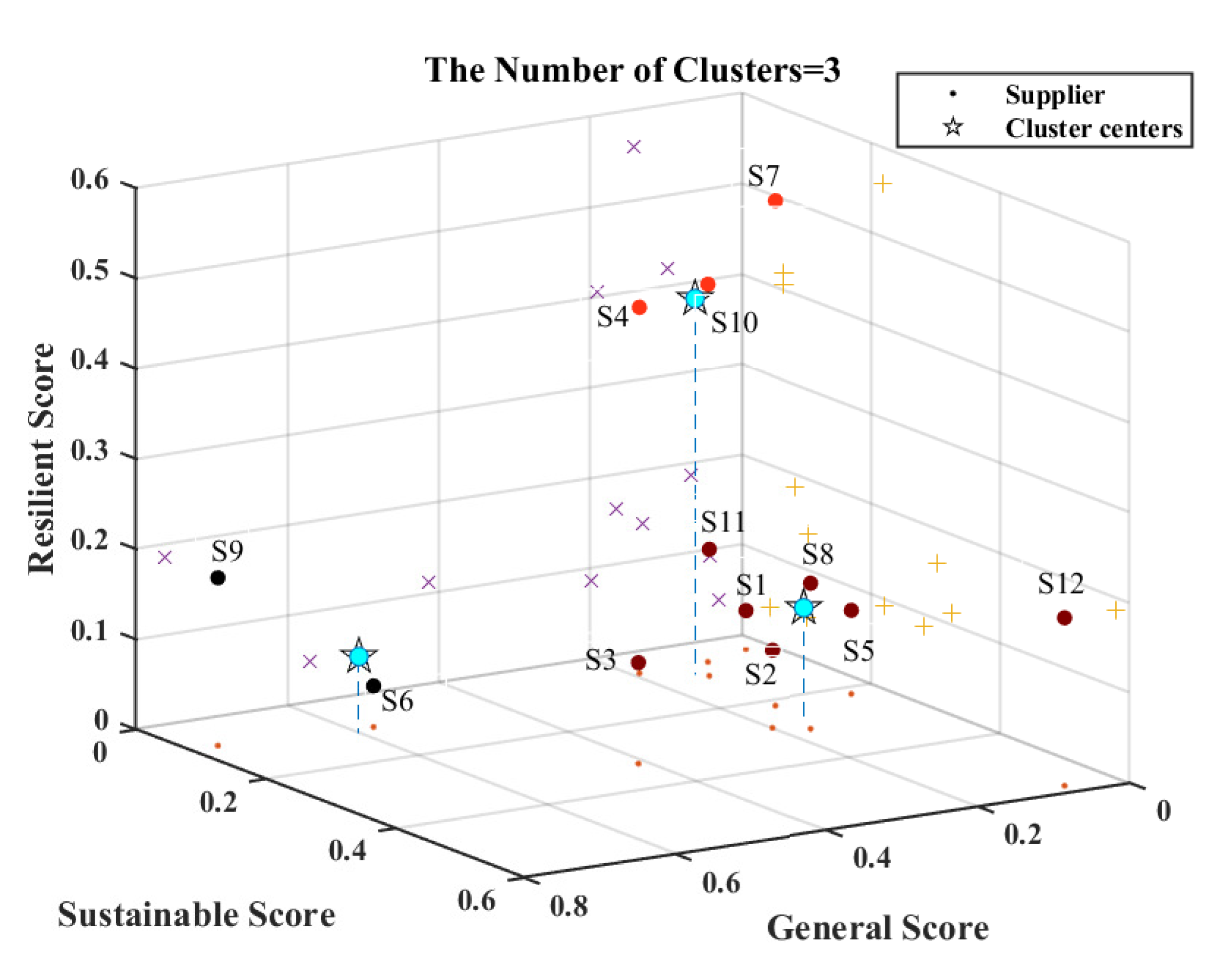
The results of supplier clustering using PFCM are shown in Figure 4. As depicted in Figure 4, the algorithm classifies suppliers into three clusters based on their normalized scores in the general, sustainable, and resilient dimensions. Suppliers S4, S7, and S10 are classified as the most resilient-sustainable suppliers, while suppliers S6 and S9 are classified as the second category of suppliers with lower overall resilient-sustainable performance. The suppliers in the third group failed to meet the minimum requirements for resilient-sustainable performance and were therefore removed from the candidate supplier list. The multi-objective mixed-possibilistic programming model developed in Section 3.3 was solved to determine the purchase decision for each supplier under different disruption scale scenarios. For different priority objective functions, different optimal values of the LAM model can be obtained, where $\lambda =0.5$, $v={10}^{-4}$, and ${\delta }_i=1.0$. For different priority objective functions,

Table 7. The percentage of raw material purchased from each supplier at different optimization of the objective functions.

Scenarios	Disruption Scale	Supplier
		S4	S6	S7	S9	S10
CS1 $min{f}_1$	Small	96	53	95	70	94
	Medium	22	58	12	49	21
	Large	48	89	47		36
CS2 $max{f}_2$	Small	71	94	72	61
	Medium	64	91	87
	Large	68		46	40	49
CS3 $max{f}_3$	Small	41	95	46		94
	Medium	92	74	94	73	98
	Large	58	34	47	49	16

shows the percentage of purchased raw materials from each supplier under different disruption scales.

The relative optimal order of the objective function has a significant impact on the final sourcing decision, which in turn affects the overall operational performance of the supply chain. Table 7 shows that the augmented $\epsilon$-constraint method is used to optimize three priority objective functions (i.e., the cost objective (CS1), sustainable objective (CS2), and resilience objective (CS3)) under different disruption scales to obtain the percentage of capacity utilization of each supplier, which reflects the level of participation of each supplier. In all scenarios, primary suppliers and backup suppliers are almost exclusively utilized for the procurement of raw materials. Our observation indicates that suppliers S4 and S7 were selected as the most effective supplier in almost all scenarios, and some suppliers were selected in specific scenarios (i.e., S6, S9, and S10). The level of supplier participation obviously depends on its performance in three dimensions: cost, sustainability, and resilience. When the emphasis is on cost objectives and the ability to withstand small-scale disruptions, suppliers S4, S7, and S10 are preferred. When sustainable objectives are emphasized, suppliers S4 and S7 are considered effective in their ability to deal with disruptions across all three scales. If resilience objectives are emphasized, all suppliers except for S9 demonstrate excellent resilience performance. Meanwhile, we observe that in all scenario configurations, S4 and S7 can effectively cope with disruptions of different scales, and they can maintain cost effectiveness while also achieving sustainability and resilience. Therefore, we can conclude that suppliers S4 and S7 are better suited for establishing a resilient and sustainable supply base.

5.3. Analysis of the Trade-Off between Performance and Disruption Scales

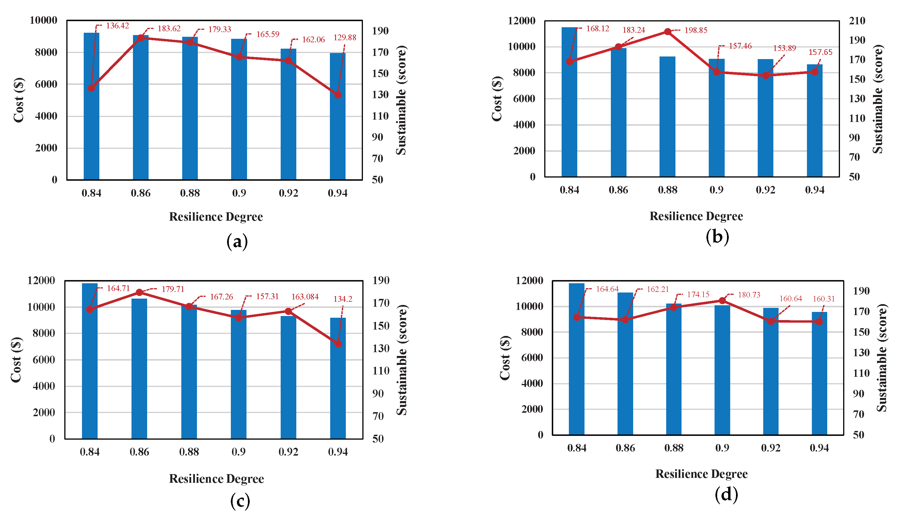
This section presents an analysis of the trade-offs between supply chain performance and disruption scales, with the aim of exploring the relationship between cost, sustainable, and resilience objectives across different disruption scales. This trade-off can be achieved by adjusting the degree of resilience (${\epsilon }_{res}$), and using the cost and sustainable objectives as the priority objective solution model, respectively. The results are presented in Figure 5, which illustrates the trade-offs between cost, sustainable, and resilience objectives across different disruption scenarios, including the following: (a) the baseline scenario with no disruption, (b) small-scale disruptions only, (c) medium-scale disruptions only, and (d) large-scale disruptions only.

As shown in Figure 5, the cost objective increases with the expansion of the disruption scale, and the cost is lowest in the baseline scenario with no disruption. Furthermore, we observe that as the degree of resilience increases, the cost objective of the supply chain decreases, while the sustainable objective first improves and then declines. When the resilience of the supply chain is low, the supply chain tends to collaborate with suppliers that demonstrate strong performance in both resilience and sustainability, even if their costs are higher. When the supply chain has high flexibility to cope with random disruptions, it tends to engage with lower-cost suppliers, even if their performance in terms of resilience and sustainability is low. Interestingly, the cost objective decreases in a linear pattern as the resilience of the supply chain increases.

By focusing on disruption scales, further insights can be gained into the relationship between cost, sustainable, and resilience objectives. Analysis results from Figure 5a–d indicate that improving the resilience of the supply chain leads to a reduction in the supply chain’s cost objective and significant changes in sustainable performance. As shown in Figure 5c, if the resilience is improved from 0.90 to 0.94, the sustainability of the supply chain will be greatly affected during medium-scale disruptions. In contrast to Figure 5c, it can be seen in Figure 5b that increasing the resilience from 0.90 to 0.94 only leads to a slight change in the sustainable performance of the supply chain. Similar observations can be made for large-scale disruptions in Figure 5d, where increasing resilience from 0.90 to 0.94 leads to only a minor reduction in sustainable performance. The results suggest that it may be possible to improve the resilience of the supply chain while preserving cost efficiency and sustainable performance under certain disruption scenarios.

5.4. Network Robustness Experiment

To further verify the robustness of the proposed network structure, performance comparison results were obtained from three network structures: (1) multi-source (conclude the primary supplier and the backup supplier) PI logistics system (MS-PI); (2) multi-source (conclude the primary supplier and the backup supplier) collaborative logistics system (MS-CO); and (3) multi-source (conclude the primary supplier) PI logistics system (PS-PI). In MS-CO, collaboration is established among enterprises that share similar annual throughput and geographic location of market zones. It is noteworthy that in MS-CO, vehicles can extract products from all plants and deliver them directly to the market zones. Consolidation and de-consolidation of products are only carried out at the plants and market zones. MS-PI and PS-PI differ from MS-CO in that products can be transported from the plant to one or more PI hubs via multiple vehicles, and are then consolidated and deconsolidated multiple times before being shipped to the market zone. Specifically, all network configurations take into account the additional capacity added by the plant. It is noteworthy that, compared to the PS-PI and MS-CO networks, the MS-PI network emphasizes the value of backup suppliers and PI in the supply chain network. Additionally, we use the same data for experiments in all test cases.

Experiments were conducted on three network structures, exploring the impact of different disruption scales (none, small, medium, and large) on each network’s performance. To provide a clearer illustration of the results,

Table 8. Payoff table obtained by the lexicographic optimization of the objective functions.

Scenarios	Disruption Scale	Cost			Sustainable Performance			Resilience
		MS-PI	MS-CO	SS-PI	MS-PI	MS-CO	SS-PI	MS-PI	MS-CO	SS-PI
CS1 $min{f}_1$	Small	10,608	13,450	12,881	170.22	180.10	178.64	0.8933	0.8657	0.8712
	Medium	10,713	13,550	13,421	198.39	200.10	196.63	0.8363	0.8999	0.8452
	Large	13,025	14,026	14,021	233.44	250.00	226.85	0.8309	0.8858	0.8165
CS2 $max{f}_2$	Small	9843.9	13,361	10,213	179.97	170.93	163.38	0.8706	0.8749	0.8675
	Medium	10,532	13,418	10,982	195.60	179.99	180.11	0.8717	0.8858	0.8276
	Large	10,932	14,016	11,579	194.64	190.46	185.20	0.8958	0.8973	0.8104
CS3 $max{f}_3$	Small	8273.7	13,304	10,213	175.61	170.08	163.38	0.9722	0.8861	0.8675
	Medium	9378.7	13,709	10,982	187.56	187.05	180.11	0.9909	0.8699	0.8276
	Large	9521.3	13,868	11,579	194.93	190.02	197.23	0.8914	0.8759	0.8535

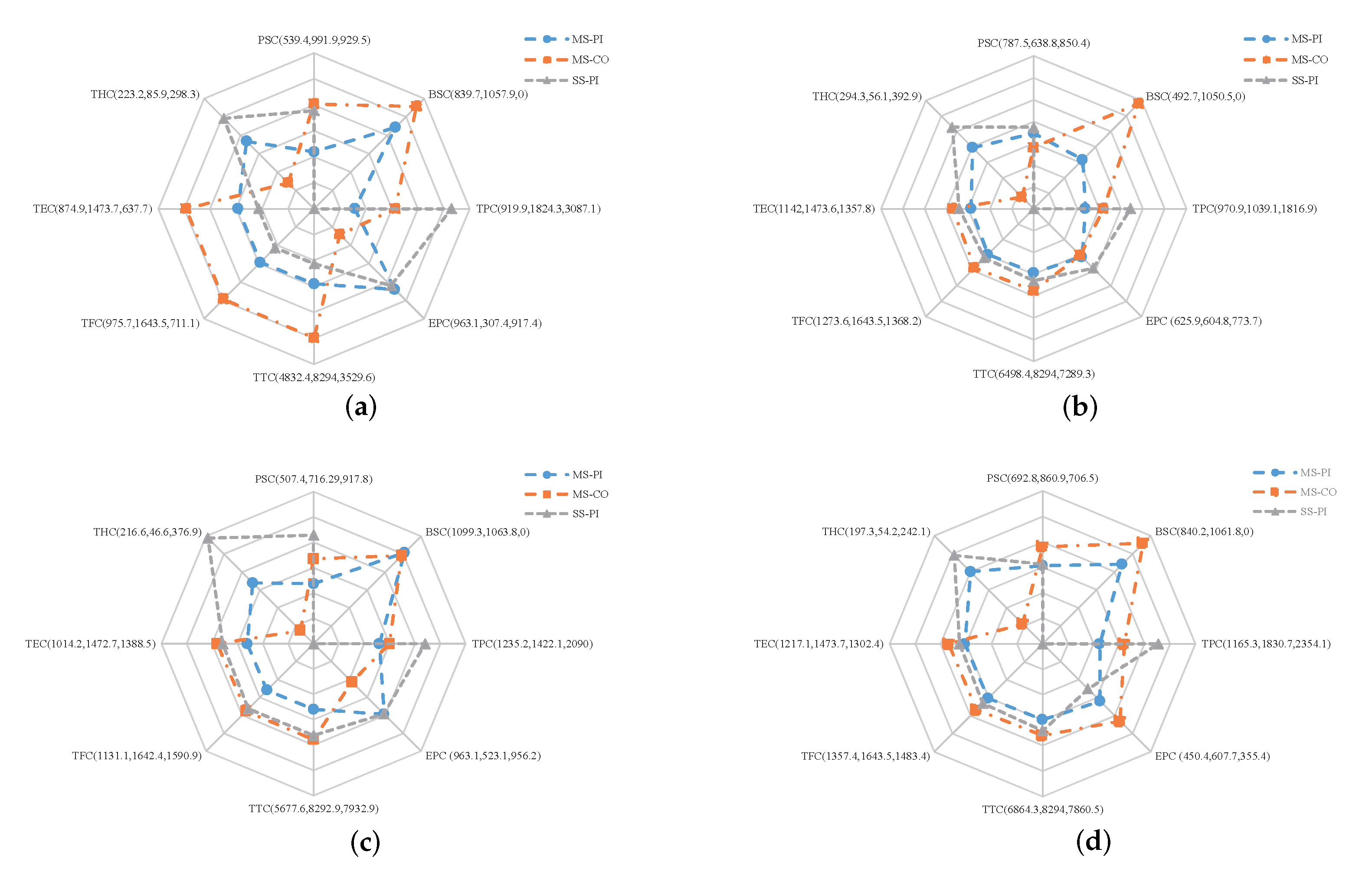
presents a comparison of cost, sustainability, and resilience among MS-PI, MS-CO, and SS-PI under different priority objective functions and disruption scales. Figure 6, Figure 7 and Figure 8 display the results of the four disruption scale test cases using a radar chart, with the costs of MS-PI, MS-CO, and SS-PI represented by the numbers in parentheses. The key performance indicators (KPIs) for different network configurations are as follows: PSC (total primary supplier cost), BSC (total backup supplier cost), TPC (total production cost), EPC (extra production cost), TTC (total transportation cost), TFC (total fuel cost), TEC (total emission cost), and THC (total holding cost). Each network structure’s cost configuration is indicated by a clear line pattern, with closer lines to the center indicating lower costs. The percentage difference between MS-PI and MS-CO (or PS-PI) is calculated as follows: % improvement with MS-PI over MS-CO(SS-PI) $=\frac{F_{MS-CO\left(SS-PI\right)}^{\ast }-F_{MS-PI}^{\ast }}{F_{MS-PI}^{\ast }}\times 100\%$ where $F_{\left(\ast \right)}^{\left(\#\right)}$ indicates the cost, sustainability, and resilience $(\#)$ of the corresponding network structure $(\ast )$.

Based on the data presented in Table 8 and Figure 6, Figure 7 and Figure 8, the following conclusions can be drawn. Table 8 confirms that the order of cost is MS-PI, PS-PI, and MS-CO, with MS-PI having the lowest cost and MS-CO having the highest cost. In essence, it has been observed in both theory and practice that an increase in the flexibility and robustness of the network structure leads to an increase in cost effectiveness. Additionally, we note that backup suppliers and PI are highly effective in addressing disruptions of varying scales.

As specified in Figure 6, in CS1, compared with MS-CO, MS-PI and SS-PI have lower transportation, fuel, and emission costs, regardless of the scale of the disruption. However, the interesting finding is that the handling costs of both MS-PI and PS-PI are higher. This may be attributed to the fact that PI containers may need to be deconsolidated and reconsolidated at each transportation node of MS-PI and SS-PI, which enhances transportation efficiency and vehicle utilization, effectively reducing fuel costs, emission costs, and transportation costs. Meanwhile, as transportation efficiency improves, the deconsolidation and reconsolidation of PI containers result in an increase in handling costs. Compared with PS-PI, MS-PI’s supplier base is set up as "mixed", including primary suppliers and backup suppliers. Despite the increased cost of BSC in MS-PI, the overall cost effectiveness of the supply chain improved due to its diverse supply. Therefore, MS-PI can provide a more competitive solution regardless of the scale of the disruption.

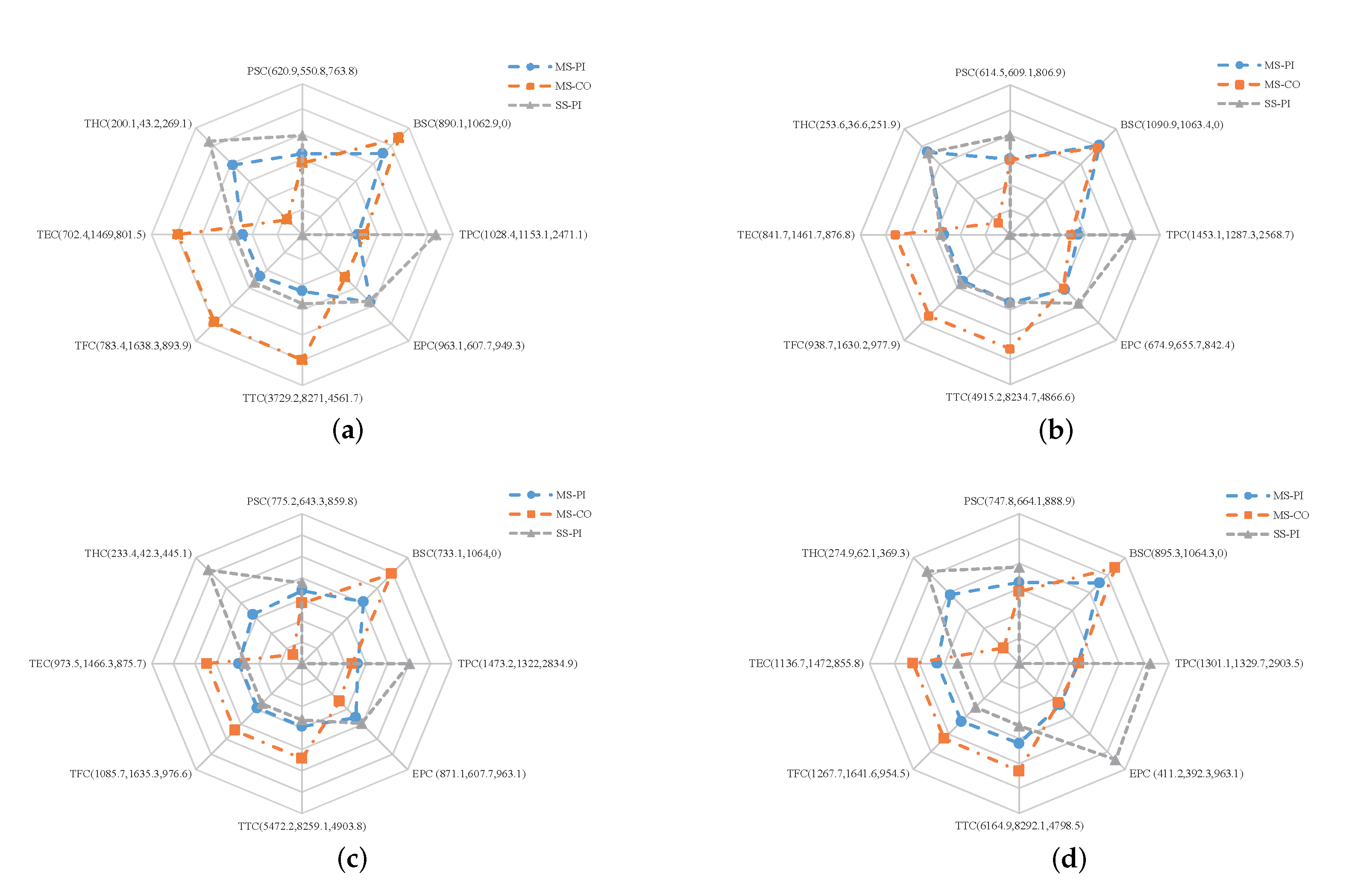
CS2 provides more sustainable operational planning options, as shown in Figure 7. Comparison with MS-CO revealed that MS-PI demonstrated a sustainable performance improvement of 5.02%, 7.98%, and 2.15% under small, medium, and large disruption scales, respectively. Significantly, in the comparison between PS-PI and MS-PI, the latter demonstrated an improvement in sustainable performance of 9.22%, 7.92%, and 4.85% under small, medium, and large disruption scales, respectively. The main reason for this beneficial change in MS-PI mainly derived from the diversity and flexibility of the supply base and the interconnection characteristics of PI. The presence of backup suppliers in MS-PI leads to an increase in the diversity of the supply base. The efficient operation of PI encourages the supply chain to collaborate with suppliers that exhibit good resilient and sustainable performance, thus expediting the sustainable development of the supply chain. Thus, MS-PI enhances the sustainable performance of the supply chain while simultaneously improving cost efficiency, owing to its abundant supply base.

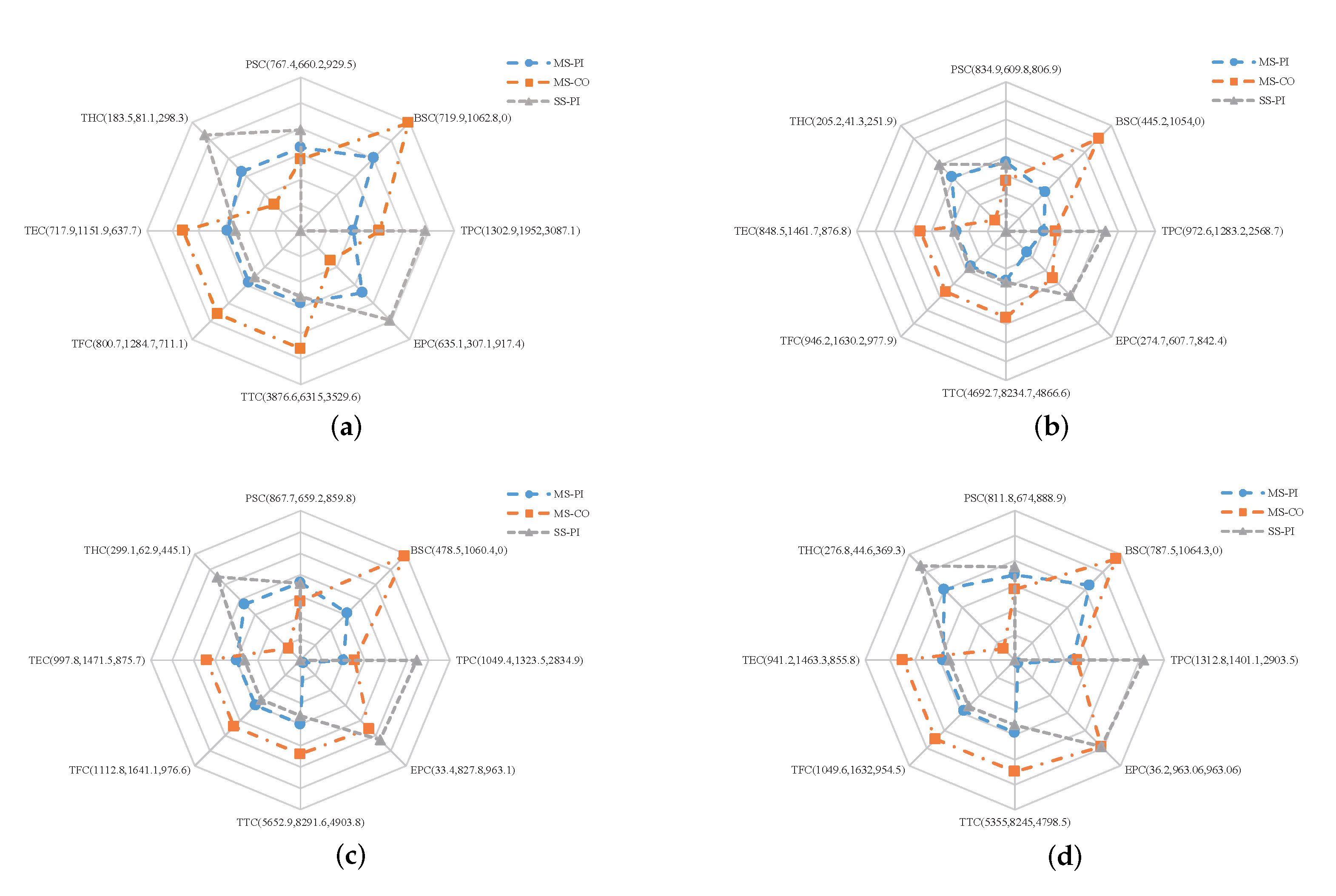
CS3 provides a more flexible operation plan based on the resilience objective as the priority objective function. Based on the results shown in Figure 8, we observed that MS-PI outperforms both MS-CO and PS-PI in terms of resilience, cost efficiency, and sustainable performance, regardless of the competitive network. Therefore, MS-PI can mitigate disruptions without compromising economic costs and sustainable performance. Notably, when comparing MS-CO and MS-PI under three levels of destruction, the cost of MS-PI improved by 60.80%, 46.17%, and 45.65%, respectively. Additionally, the sustainable performance of MS-PI improved by 3.15%, 0.3%, and 2.52%, while its resilience increased by 8.86%, 12.21%, and 15.70%, respectively. In the comparison of PS-PI and MS-PI under the three disruption scales, compared with the slight improvement in MS-PI’s sustainable performance (improvements of 6.96%, 3.97%, and 4.50%, respectively), the resilience of MS-PI was significantly improved by 10.77%, 16.48%, and 17.60% and the cost improvement was 23.44%, 17.10%, and 21.61%, respectively. The resilience advantage of MS-PI is primarily achieved through the use of backup suppliers, as well as the high integration, flexibility, and openness of PI. Backup suppliers can prevent shortages, strikes, disruptions from primary suppliers, and capacity problems that primary suppliers may encounter. PI can leverage the interconnectivity and synergies between entities in the supply chain network to integrate dispersed and overlapping transportation flows. This enhances the flexibility and resilience of the transportation network. Meanwhile, we can observe that the cost efficiency and sustainable performance of MS-PI are higher than that of MS-CO and SS-PI. When random disruptions occur at suppliers, plants, and PI hubs, MS-PI can always respond to disruptions quickly with the minimal cost and the best sustainable performance, regardless of the scale of the disruption. Thus, MS-PI enhances the flexibility and resilience of the supply chain network while maintaining cost efficiency and sustainable performance. Considering the various disruption scenarios, it is clear that greater flexibility in the supply chain network structure would be beneficial.

6. Conclusions and Future Work

The study of supply chain resilience and sustainability has become an important focus of academic research. While a significant amount of modeling work has explored different aspects of supply chain resilience and sustainability, these studies primarily focused on traditional supply chain networks and their interrelationships and potential interactions. At present, there is no literature in PI that jointly explores these two topics to obtain a PI-enabled resilient and sustainable supply chain network design. The major thrust of this paper is to conduct an early attempt at resilient and sustainable analysis in the PI-enabled supply chain. By modeling the key operational features of PI, a hybrid method is proposed to solve the PI-enabled supply–production–distribution problem with integrated resilience and sustainability analysis. The proposed approach is implemented in two phases. Firstly, based on the decision makers, the first stage of the hybrid method proposes the PFCM to evaluate the resilient-sustainable performance of each supplier (primary and backup suppliers). Secondly, with the obtained supplier’s performance score as an input parameter, a multi-objective mixed-possibilistic programming model was developed in the second stage, which integrates the three dimensions of cost, sustainability, and resilience. Next, we re-developed the multi-objective model based on the multi-objective mixed-possibilistic model to account for uncertainties in demand, cost, and other factors. The augmented $\epsilon$-constraint method was employed to optimize the equivalent crisp model, and to obtain the trade-off among the three objective functions by identifying the optimal solution from the Pareto optimal set. The developed model’s applicability was verified through numerical experiments.

The following main conclusions are drawn from the experimental results: Firstly, suppliers with good resilient-sustainable performance are crucial for mitigating supply chain disruption and enhancing the resilience and sustainability of the supply chain at the source. Secondly, traditional supply chains are more susceptible to disruptions in terms of three key dimensions: cost, sustainability, and resilience, compared to PI-enabled supply chain configurations. Furthermore, the incorporation of backup suppliers and PI can enhance the resilience of the supply chain, enabling sustainable performance across different scales of disruption without incurring significant cost changes. Thirdly, from a long-term perspective, the robust MS-PI is the most efficient, sustainable, and resilient supply chain structure. Fourthly, from a strategic perspective, supporting PI-enabled supply chains is more valuable than supporting traditional supply chains (in terms of supply chain cost, sustainability, and resilience).

Based on the previous analysis, the main management insights can be summarized as follows: Firstly, the developed PI-enabled supply–production–distribution model can help companies improve supply chain resilience and respond to increasing sustainability requirements. Secondly, the supplier performance analysis conducted in this article can help decision makers understand the importance of comprehensive business decisions. The proposed model can help managers integrate purchasing, production, and distribution decisions to address the optimization problem of several conflicting objectives, enabling managers to determine the best business solution. Thirdly, the value of backup procurement should be emphasized, as backup suppliers can mitigate supply uncertainty and prevent supply shortages during disruptions. The role of PI should also be emphasized, as open sharing between PI hubs has brought improvements in supply chain cost efficiency, sustainable, and resilience. Finally, implementing PI-enabled supply chains can help ensure the resilient and sustainable development of enterprises, benefitting society and the environment while also providing resilience advantages.

As a guide for future research, the study presented in this article can be extended further. Considering the transportation disruption of PI-enabled supply chains, evaluating PI’s resilient performance from a more comprehensive perspective may be an interesting direction for future research. Additionally, considering the uncertainties of suppliers, plants, PI hubs, and market zones’ capabilities can be another idea for future research. Lastly, the development of an efficient and accurate solution method is also a good direction for future research.

References

1. Ho, W.; Zheng, T.; Yildiz, H.; Talluri, S. Supply chain risk management: A literature review. Int. J. Prod. Res. 2015, 53, 5031–5069. [Google Scholar] [CrossRef]
2. He, J.; Alavifard, F.; Ivanov, D.; Jahani, H. A real-option approach to mitigate disruption risk in the supply chain. Omega 2019, 88, 133–149. [Google Scholar] [CrossRef]
3. Tang, C.S. Perspectives in supply chain risk management. Int. J. Prod. Econ. 2006, 103, 451–488. [Google Scholar] [CrossRef]
4. Baghersad, M.; Zobel, C.W. Assessing the extended impacts of supply chain disruptions on firms: An empirical study. Int. J. Prod. Econ. 2021, 231, 107862. [Google Scholar] [CrossRef]
5. Mehrjerdi, Y.Z.; Shafiee, M. A resilient and sustainable closed-loop supply chain using multiple sourcing and information sharing strategies. J. Clean. Prod. 2021, 289, 125141. [Google Scholar] [CrossRef]
6. Tomlin, B. On the Value of Mitigation and Contingency Strategies for Managing Supply Chain Disruption Risks. Manag. Sci. 2006, 52, 639–657. [Google Scholar] [CrossRef] [Green Version]
7. Soni, U.; Jain, V.; Kumar, S. Measuring supply chain resilience using a deterministic modeling approach. Comput. Ind. Eng. 2014, 74, 11–25. [Google Scholar] [CrossRef]
8. Torabi, S.; Baghersad, M.; Mansouri, S. Resilient supplier selection and order allocation under operational and disruption risks. Transp. Res. Part E Logist. Transp. Rev. 2015, 79, 22–48. [Google Scholar] [CrossRef]
9. Namdar, J.; Li, X.; Sawhney, R.; Pradhan, N. Supply chain resilience for single and multiple sourcing in the presence of disruption risks. Int. J. Prod. Res. 2018, 56, 2339–2360. [Google Scholar] [CrossRef] [Green Version]
10. Jabbarzadeh, A.; Fahimnia, B.; Sabouhi, F. Resilient and sustainable supply chain design: Sustainability analysis under disruption risks. Int. J. Prod. Res. 2018, 56, 5945–5968. [Google Scholar] [CrossRef]
11. Ivanov, D. Revealing interfaces of supply chain resilience and sustainability: A simulation study. Int. J. Prod. Res. 2018, 56, 3507–3523. [Google Scholar] [CrossRef] [Green Version]
12. Fahimnia, B.; Jabbarzadeh, A. Marrying supply chain sustainability and resilience: A match made in heaven. Transp. Res. Part E Logist. Transp. Rev. 2016, 91, 306–324. [Google Scholar] [CrossRef]
13. Zahiri, B.; Zhuang, J.; Mohammadi, M. Toward an integrated sustainable-resilient supply chain: A pharmaceutical case study. Transp. Res. Part E Logist. Transp. Rev. 2017, 103, 109–142. [Google Scholar] [CrossRef]
14. Negri, M.; Cagno, E.; Colicchia, C.; Sarkis, J. Integrating sustainability and resilience in the supply chain: A systematic literature review and a research agenda. Bus. Strategy Environ. 2021, 30, 2858–2886. [Google Scholar] [CrossRef]
15. Vali-Siar, M.M.; Roghanian, E. Sustainable, resilient and responsive mixed supply chain network design under hybrid uncertainty with considering COVID-19 pandemic disruption. Sustain. Prod. Consum. 2022, 30, 278–300. [Google Scholar] [CrossRef]
16. Negri, M.; Cagno, E.; Colicchia, C. Building sustainable and resilient supply chains: A framework and empirical evidence on trade-offs and synergies in implementation of practices. Prod. Plan. Control 2022, 1–24. [Google Scholar] [CrossRef]
17. Montreuil, B. Toward a Physical Internet: Meeting the global logistics sustainability grand challenge. Logist. Res. 2011, 3, 71–87. [Google Scholar] [CrossRef]
18. Pan, S.; Ballot, E.; Huang, G.Q.; Montreuil, B. Physical Internet and interconnected logistics services: Research and applications. Int. J. Prod. Res. 2017, 55, 2603–2609. [Google Scholar] [CrossRef]
19. Montreuil, B.; Buckley, S.; Faugere, L.; Khir, R.; Derhami, S. Urban parcel logistics hub and network design: The impact of modularity and hyperconnectivity. In Proceedings of the 15th IMHRC Proceedings, Savannah, GA, USA, 23–26 July 2018. [Google Scholar]
20. Kulkarni, O.; Dahan, M.; Montreuil, B. Resilient hyperconnected parcel delivery network design under disruption risks. Int. J. Prod. Econ. 2022, 251, 108499. [Google Scholar] [CrossRef]
21. Montreuil, B.; Meller, R.D.; Ballot, E. Physical Internet Foundations. In Service Orientation in Holonic and Multi Agent Manufacturing and Robotics; Springer: Berlin/Heidelberg, Germany, 2013; pp. 151–166. [Google Scholar]
22. Ballot, E.; Montreuil, B.; Meller, R. The Physical Internet; La Documentation Française: Paris, France, 2014. [Google Scholar]
23. Crainic, T.G.; Montreuil, B. Physical Internet Enabled Hyperconnected City Logistics. Transp. Res. Procedia 2016, 12, 383–398. [Google Scholar] [CrossRef] [Green Version]
24. Ben Mohamed, I.; Klibi, W.; Labarthe, O.; Deschamps, J.C.; Babai, M.Z. Modelling and Solution Approaches for the Interconnected City Logistics. Int. J. Prod. Res. 2017, 55, 2664–2684. [Google Scholar] [CrossRef]
25. Sarraj, R.; Ballot, E.; Pan, S.; Hakimi, D.; Montreuil, B. Interconnected Logistic Networks and Protocols: Simulation-Based Efficiency Assessment. Int. J. Prod. Res. 2014, 52, 3185–3208. [Google Scholar] [CrossRef]
26. Pan, S.; Nigrelli, M.; Ballot, E.; Sarraj, R.; Yang, Y. Perspectives of Inventory Control Models in the Physical Internet: A Simulation Study. Comput. Ind. Eng. 2015, 84, 122–132. [Google Scholar] [CrossRef]
27. Peng, X.S.; Ji, S.F.; Ji, T.T. Promoting Sustainability of the Integrated Production-Inventory-Distribution System through the Physical Internet. Int. J. Prod. Res. 2020, 58, 1–20. [Google Scholar] [CrossRef]
28. Yang, Y.; Pan, S.; Ballot, E. Mitigating supply chain disruptions through interconnected logistics services in the Physical Internet. Int. J. Prod. Res. 2017, 55, 3970–3983. [Google Scholar] [CrossRef]
29. Olan, F.; Liu, S.; Suklan, J.; Jayawickrama, U.; Arakpogun, E.O. The role of Artificial Intelligence networks in sustainable supply chain finance for food and drink industry. Int. J. Prod. Res. 2022, 60, 4418–4433. [Google Scholar] [CrossRef]
30. Yousefi, S.; Tosarkani, B.M. An analytical approach for evaluating the impact of blockchain technology on sustainable supply chain performance. Int. J. Prod. Econ. 2022, 246, 108429. [Google Scholar] [CrossRef]
31. Govindan, K.; Rajeev, A.; Padhi, S.S.; Pati, R.K. Supply Chain Sustainability and Performance of Firms: A Meta-Analysis of the Literature. Transp. Res. Part E Logist. Transp. Rev. 2020, 137, 101923. [Google Scholar] [CrossRef]
32. Thies, C.; Kieckhäfer, K.; Spengler, T.S.; Sodhi, M.S. Operations Research for Sustainability Assessment of Products: A Review. Eur. J. Oper. Res. 2019, 274, 1–21. [Google Scholar] [CrossRef]
33. Barbosa-Póvoa, A.P.F.D.; da Silva, C.; Carvalho, A. Opportunities and challenges in sustainable supply chain: An operations research perspective. Eur. J. Oper. Res. 2018, 268, 399–431. [Google Scholar] [CrossRef]
34. Chen, S.; Hayat, K.; Yang, X. Upper Bounded Minimal Solution of the Max-Min Fuzzy Relation Inequality System. IEEE Access 2022, 10, 84384–84397. [Google Scholar] [CrossRef]
35. Xiao, G.; Hayat, K.; Yang, X. Evaluation and its derived classification in a Server-to-Client architecture based on the fuzzy relation inequality. Fuzzy Optim. Decis. Mak. 2022, 1–33. [Google Scholar] [CrossRef]
36. Hosseini, Z.S.; Flapper, S.D.; Pirayesh, M. Sustainable supplier selection and order allocation under demand, supplier availability and supplier grading uncertainties. Comput. Ind. Eng. 2022, 165, 107811. [Google Scholar] [CrossRef]
37. Shang, Z.; Yang, X.; Barnes, D.; Wu, C. Supplier selection in sustainable supply chains: Using the integrated BWM, fuzzy Shannon entropy, and fuzzy MULTIMOORA methods. Expert Syst. Appl. 2022, 195, 116567. [Google Scholar] [CrossRef]
38. Mohammed, A.; Harris, I.; Govindan, K. A hybrid MCDM-FMOO approach for sustainable supplier selection and order allocation. Int. J. Prod. Econ. 2019, 217, 171–184. [Google Scholar] [CrossRef]
39. Awasthi, A.; Govindan, K.; Gold, S. Multi-tier sustainable global supplier selection using a fuzzy AHP-VIKOR based approach. Int. J. Prod. Econ. 2018, 195, 106–117. [Google Scholar] [CrossRef] [Green Version]
40. Zimmer, K.; Fröhling, M.; Schultmann, F. Sustainable supplier management–a review of models supporting sustainable supplier selection, monitoring and development. Int. J. Prod. Res. 2016, 54, 1412–1442. [Google Scholar] [CrossRef]
41. Naderi, R.; Nikabadi, M.S.; Tabriz, A.A.; Pishvaee, M.S. Supply chain sustainability improvement using exergy analysis. Comput. Ind. Eng. 2021, 154, 107142. [Google Scholar] [CrossRef]
42. Mani, V.; Jabbour, C.J.C.; Mani, K.T. Supply chain social sustainability in small and medium manufacturing enterprises and firms’ performance: Empirical evidence from an emerging Asian economy. Int. J. Prod. Econ. 2020, 227, 107656. [Google Scholar] [CrossRef]
43. Vivas, R.D.C.; Sant’Anna, A.M.O.; Esquerre, K.P.O.; Freires, F.G.M. Integrated method combining analytical and mathematical models for the evaluation and optimization of sustainable supply chains: A Brazilian case study. Comput. Ind. Eng. 2020, 139, 105670. [Google Scholar] [CrossRef]
44. Zarbakhshnia, N.; Kannan, D.; Mavi, R.K.; Soleimani, H. A novel sustainable multi-objective optimization model for forward and reverse logistics system under demand uncertainty. Ann. Oper. Res. 2020, 295, 843–880. [Google Scholar] [CrossRef]
45. Mota, B.; Gomes, M.I.; Carvalho, A.; Barbosa-Povoa, A.P. Sustainable supply chains: An integrated modeling approach under uncertainty. Omega 2018, 77, 32–57. [Google Scholar] [CrossRef]
46. Luthra, S.; Govindan, K.; Mangla, S.K. Structural model for sustainable consumption and production adoption—A grey-DEMATEL based approach. Resour. Conserv. Recycl. 2017, 125, 198–207. [Google Scholar] [CrossRef]
47. Boukherroub, T.; Ruiz, A.; Guinet, A.; Fondrevelle, J. An integrated approach for sustainable supply chain planning. Comput. Oper. Res. 2015, 54, 180–194. [Google Scholar] [CrossRef]
48. Pishvaee, M.; Razmi, J.; Torabi, S. An accelerated Benders decomposition algorithm for sustainable supply chain network design under uncertainty: A case study of medical needle and syringe supply chain. Transp. Res. Part E Logist. Transp. Rev. 2014, 67, 14–38. [Google Scholar] [CrossRef]
49. Brandenburg, M.; Govindan, K.; Sarkis, J.; Seuring, S. Quantitative models for sustainable supply chain management: Developments and directions. Eur. J. Oper. Res. 2014, 233, 299–312. [Google Scholar] [CrossRef]
50. Seuring, S. A review of modeling approaches for sustainable supply chain management. Decis. Support Syst. 2013, 54, 1513–1520. [Google Scholar] [CrossRef]
51. Soleimani, H.; Chhetri, P.; Fathollahi-Fard, A.M.; Mirzapour Al-e Hashem, S.; Shahparvari, S. Sustainable closed-loop supply chain with energy efficiency: Lagrangian relaxation, reformulations and heuristics. Ann. Oper. Res. 2022, 318, 531–556. [Google Scholar] [CrossRef]
52. Tirkolaee, E.B.; Goli, A.; Ghasemi, P.; Goodarzian, F. Designing a sustainable closed-loop supply chain network of face masks during the COVID-19 pandemic: Pareto-based algorithms. J. Clean. Prod. 2022, 333, 130056. [Google Scholar] [CrossRef]
53. Yu, H.; Solvang, W.D. A fuzzy-stochastic multi-objective model for sustainable planning of a closed-loop supply chain considering mixed uncertainty and network flexibility. J. Clean. Prod. 2020, 266, 121702. [Google Scholar] [CrossRef]
54. Nayeri, S.; Paydar, M.M.; Asadi-Gangraj, E.; Emami, S. Multi-objective fuzzy robust optimization approach to sustainable closed-loop supply chain network design. Comput. Ind. Eng. 2020, 148, 106716. [Google Scholar] [CrossRef]
55. Sahebjamnia, N.; Fathollahi-Fard, A.M.; Hajiaghaei-Keshteli, M. Sustainable tire closed-loop supply chain network design: Hybrid metaheuristic algorithms for large-scale networks. J. Clean. Prod. 2018, 196, 273–296. [Google Scholar] [CrossRef]
56. MA, R.; YAO, L.; JIN, M.; REN, P.; LV, Z. Robust environmental closed-loop supply chain design under uncertainty. Chaos Solitons Fractals 2016, 89, 195–202. [Google Scholar] [CrossRef]
57. Fahimnia, B.; Reisi, M.; Paksoy, T.; Özceylan, E. The implications of carbon pricing in Australia: An industrial logistics planning case study. Transp. Res. Part D Transp. Environ. 2013, 18, 78–85. [Google Scholar] [CrossRef]
58. Bechtsis, D.; Tsolakis, N.; Iakovou, E.; Vlachos, D. Data-driven secure, resilient and sustainable supply chains: Gaps, opportunities, and a new generalised data sharing and data monetisation framework. Int. J. Prod. Res. 2022, 60, 4397–4417. [Google Scholar] [CrossRef]
59. Zhang, Q.; Shah, N.; Wassick, J.M.; Helling, R.; van Egerschot, P. Sustainable supply chain optimisation: An industrial case study. Comput. Ind. Eng. 2014, 74, 68–83. [Google Scholar] [CrossRef]
60. Varsei, M.; Polyakovskiy, S. Sustainable Supply Chain Network Design: A Case of the Wine Industry in Australia. Omega 2017, 66, 236–247. [Google Scholar] [CrossRef]
61. Govindan, K.; Gholizadeh, H. Robust Network Design for Sustainable-Resilient Reverse Logistics Network Using Big Data: A Case Study of End-of-Life Vehicles. Transp. Res. Part E Logist. Transp. Rev. 2021, 149, 102279. [Google Scholar] [CrossRef]
62. Rozhkov, M.; Ivanov, D.; Blackhurst, J.; Nair, A. Adapting supply chain operations in anticipation of and during the COVID-19 pandemic. Omega 2022, 110, 102635. [Google Scholar] [CrossRef] [PubMed]
63. Sawik, T. Stochastic optimization of supply chain resilience under ripple effect: A COVID-19 pandemic related study. Omega 2022, 109, 102596. [Google Scholar] [CrossRef]
64. Spieske, A.; Gebhardt, M.; Kopyto, M.; Birkel, H. Improving resilience of the healthcare supply chain in a pandemic: Evidence from Europe during the COVID-19 crisis. J. Purch. Supply Manag. 2022, 28, 100748. [Google Scholar] [CrossRef]
65. Ivanov, D.; Dolgui, A. Viability of Intertwined Supply Networks: Extending the Supply Chain Resilience Angles towards Survivability. A Position Paper Motivated by COVID-19 Outbreak. Int. J. Prod. Res. 2020, 58, 2904–2915. [Google Scholar] [CrossRef] [Green Version]
66. Iftikhar, A.; Purvis, L.; Giannoccaro, I.; Wang, Y. The impact of supply chain complexities on supply chain resilience: The mediating effect of big data analytics. Prod. Plan. Control 2022, 1–21. [Google Scholar] [CrossRef]
67. Cohen, M.; Cui, S.; Doetsch, S.; Ernst, R.; Huchzermeier, A.; Kouvelis, P.; Lee, H.; Matsuo, H.; Tsay, A.A. Bespoke supply-chain resilience: The gap between theory and practice. J. Oper. Manag. 2022, 68, 515–531. [Google Scholar] [CrossRef]
68. Belhadi, A.; Kamble, S.; Fosso Wamba, S.; Queiroz, M.M. Building supply-chain resilience: An artificial intelligence-based technique and decision-making framework. Int. J. Prod. Res. 2022, 60, 4487–4507. [Google Scholar] [CrossRef]
69. Li, Y.; Zobel, C.W. Exploring Supply Chain Network Resilience in the Presence of the Ripple Effect. Int. J. Prod. Econ. 2020, 228, 107693. [Google Scholar] [CrossRef]
70. Li, Y.; Zobel, C.W.; Seref, O.; Chatfield, D. Network Characteristics and Supply Chain Resilience under Conditions of Risk Propagation. Int. J. Prod. Econ. 2020, 223, 107529. [Google Scholar] [CrossRef]
71. Kim, Y.; Chen, Y.S.; Linderman, K. Supply Network Disruption and Resilience: A Network Structural Perspective. J. Oper. Manag. 2015, 33–34, 43–59. [Google Scholar] [CrossRef] [Green Version]
72. Hosseini, S.; Ivanov, D.; Dolgui, A. Review of quantitative methods for supply chain resilience analysis. Transp. Res. Part E Logist. Transp. Rev. 2019, 125, 285–307. [Google Scholar] [CrossRef]
73. Ribeiro, J.P.; Barbosa-Póvoa, A.P.F.D. Supply Chain Resilience: Definitions and quantitative modelling approaches—A literature review. Comput. Ind. Eng. 2018, 115, 109–122. [Google Scholar] [CrossRef]
74. Yoon, J.; Talluri, S.; Yildiz, H.; Ho, W. Models for supplier selection and risk mitigation: A holistic approach. Int. J. Prod. Res. 2018, 56, 3636–3661. [Google Scholar] [CrossRef]
75. Yildiz, H.; Yoon, J.; Talluri, S.; Ho, W. Reliable Supply Chain Network Design. Decis. Sci. 2016, 47, 661–698. [Google Scholar] [CrossRef] [Green Version]
76. Saghafian, S.; Van Oyen, M.P. Compensating for Dynamic Supply Disruptions: Backup Flexibility Design. Oper. Res. 2016, 64, 390–405. [Google Scholar] [CrossRef] [Green Version]
77. Kamalahmadi, M.; Shekarian, M.; Mellat Parast, M. The impact of flexibility and redundancy on improving supply chain resilience to disruptions. Int. J. Prod. Res. 2022, 60, 1992–2020. [Google Scholar] [CrossRef]
78. Elluru, S.; Gupta, H.; Kaur, H.; Singh, S.P. Proactive and reactive models for disaster resilient supply chain. Ann. Oper. Res. 2019, 283, 199–224. [Google Scholar] [CrossRef]
79. Khalili, S.M.; Jolai, F.; Torabi, S.A. Integrated production–distribution planning in two-echelon systems: A resilience view. Int. J. Prod. Res. 2017, 55, 1040–1064. [Google Scholar] [CrossRef]
80. Mandal, S.; Sarathy, R.; Korasiga, V.; Bhattacharya, S.; Dastidar, S. Achieving supply chain resilience: The contribution of logistics and supply chain capabilities. Int. J. Disaster Resil. Built Environ. 2016, 7, 544–562. [Google Scholar] [CrossRef]
81. Scholten, K.; Schilder, S. The role of collaboration in supply chain resilience. Supply Chain. Manag. 2015, 20, 471–484. [Google Scholar] [CrossRef]
82. Merzifonluoglu, Y.; Uzgoren, E. Photovoltaic power plant design considering multiple uncertainties and risk. Ann. Oper. Res. 2018, 262, 153–184. [Google Scholar] [CrossRef]
83. Chakraborty, T.; Chauhan, S.S.; Ouhimmou, M. Mitigating supply disruption with a backup supplier under uncertain demand: Competition vs. cooperation. Int. J. Prod. Res. 2020, 58, 3618–3649. [Google Scholar] [CrossRef]
84. Hosseini, S.; Khaled, A.A. A hybrid ensemble and AHP approach for resilient supplier selection. J. Intell. Manuf. 2019, 30, 207–228. [Google Scholar] [CrossRef]
85. Kaur, H.; Singh, S.P.; Garza-Reyes, J.A.; Mishra, N. Sustainable stochastic production and procurement problem for resilient supply chain. Comput. Ind. Eng. 2020, 139, 105560. [Google Scholar] [CrossRef]
86. Pavlov, A.; Ivanov, D.; Pavlov, D.; Slinko, A. Optimization of network redundancy and contingency planning in sustainable and resilient supply chain resource management under conditions of structural dynamics. Ann. Oper. Res. 2019, 1–30. [Google Scholar] [CrossRef]
87. Chargui, T.; Bekrar, A.; Reghioui, M.; Trentesaux, D. Multi-Objective Sustainable Truck Scheduling in a Rail-Road Physical Internet Cross-Docking Hub Considering Energy Consumption. Sustainability 2019, 11, 3127. [Google Scholar] [CrossRef] [Green Version]
88. Fazili, M.; Venkatadri, U.; Cyrus, P.; Tajbakhsh, M. Physical Internet, conventional and hybrid logistic systems: A routing optimisation-based comparison using the Eastern Canada road network case study. Int. J. Prod. Res. 2017, 55, 2703–2730. [Google Scholar] [CrossRef]
89. Montreuil, B.; Rougès, J.F.; Cimon, Y.; Poulin, D. The Physical Internet and Business Model Innovation. Technol. Innov. Manag. Rev. 2012, 2, 32–37. [Google Scholar] [CrossRef]
90. Zhalechian, M.; Tavakkoli-Moghaddam, R.; Zahiri, B.; Mohammadi, M. Sustainable design of a closed-loop location-routing-inventory supply chain network under mixed uncertainty. Transp. Res. Part E Logist. Transp. Rev. 2016, 89, 182–214. [Google Scholar] [CrossRef]
91. Yang, Y.; Pan, S.; Ballot, E. Innovative vendor-managed inventory strategy exploiting interconnected logistics services in the Physical Internet. Int. J. Prod. Res. 2017, 55, 2685–2702. [Google Scholar] [CrossRef]
92. Fattahi, M.; Govindan, K. A multi-stage stochastic program for the sustainable design of biofuel supply chain networks under biomass supply uncertainty and disruption risk: A real-life case study. Transp. Res. Part E Logist. Transp. Rev. 2018, 118, 534–567. [Google Scholar] [CrossRef]
93. Mohammed, A.; Harris, I.; Soroka, A.; Nujoom, R. A hybrid MCDM-fuzzy multi-objective programming approach for a G-resilient supply chain network design. Comput. Ind. Eng. 2019, 127, 297–312. [Google Scholar] [CrossRef]
94. Sabouhi, F.; Jabalameli, M.S.; Jabbarzadeh, A. An optimization approach for sustainable and resilient supply chain design with regional considerations. Comput. Ind. Eng. 2021, 159, 107510. [Google Scholar] [CrossRef]
95. Sazvar, Z.; Tafakkori, K.; Oladzad, N.; Nayeri, S. A capacity planning approach for sustainable-resilient supply chain network design under uncertainty: A case study of vaccine supply chain. Comput. Ind. Eng. 2021, 159, 107406. [Google Scholar] [CrossRef]
96. Kim, N.; Montreuil, B.; Klibi, W.; Babai, M.Z. Network inventory deployment for responsive fulfillment. Int. J. Prod. Econ. 2022, 255, 108664. [Google Scholar] [CrossRef]
97. Guo, Z.; Wong, W.K.; Li, M. A multivariate intelligent decision-making model for retail sales forecasting. Decis. Support Syst. 2013, 55, 247–255. [Google Scholar] [CrossRef]
98. Awasthi, A.; Chauhan, S.S.; Goyal, S. A fuzzy multicriteria approach for evaluating environmental performance of suppliers. Int. J. Prod. Econ. 2010, 126, 370–378. [Google Scholar] [CrossRef]
99. Vahidi, F.; Torabi, S.A.; Ramezankhani, M. Sustainable supplier selection and order allocation under operational and disruption risks. J. Clean. Prod. 2018, 174, 1351–1365. [Google Scholar] [CrossRef]
100. Bakeshlou, E.A.; Khamseh, A.A.; Asl, M.A.G.; Sadeghi, J.; Abbaszadeh, M. Evaluating a green supplier selection problem using a hybrid MODM algorithm. J. Intell. Manuf. 2017, 28, 913–927. [Google Scholar] [CrossRef]
101. Fallahpour, A.; Udoncy Olugu, E.; Nurmaya Musa, S.; Yew Wong, K.; Noori, S. A decision support model for sustainable supplier selection in sustainable supply chain management. Comput. Ind. Eng. 2017, 105, 391–410. [Google Scholar] [CrossRef]
102. Pal, N.R.; Pal, K.; Keller, J.M.; Bezdek, J.C. A Possibilistic Fuzzy c-Means Clustering Algorithm. IEEE Trans. Fuzzy Syst. 2005, 13, 517–530. [Google Scholar] [CrossRef]
103. Barth, M.; Younglove, T.; Scora, G. Development of a Heavy-Duty Diesel Modal Emissions and Fuel Consumption Model; eScholarship: Merced, CA, USA, 2005. [Google Scholar]
104. Barth, M.; Boriboonsomsin, K. Energy and emissions impacts of a freeway-based dynamic eco-driving system. Transp. Res. Part D Transp. Environ. 2009, 14, 400–410. [Google Scholar] [CrossRef]
105. Zobel, C.W.; Khansa, L. Characterizing multi-event disaster resilience. Comput. Oper. Res. 2014, 42, 83–94. [Google Scholar] [CrossRef]
106. Xu, J.; Zhou, X. Approximation based fuzzy multi-objective models with expected objectives and chance constraints: Application to earth-rock work allocation. Inf. Sci. 2013, 238, 75–95. [Google Scholar] [CrossRef]
107. Mavrotas, G. Effective implementation of the epsilon-constraint method in Multi-Objective Mathematical Programming problems. Appl. Math. Comput. 2009, 213, 455–465. [Google Scholar] [CrossRef]
108. Cachon, G.P. Retail Store Density and the Cost of Greenhouse Gas Emissions. Manag. Sci. 2014, 60, 1907–1925. [Google Scholar] [CrossRef] [Green Version]
109. Soysal, M.; Bloemhof-Ruwaard, J.M.; Haijema, R.; van der Vorst, J.G. Modeling an Inventory Routing Problem for perishable products with environmental considerations and demand uncertainty. Int. J. Prod. Econ. 2015, 164, 118–133. [Google Scholar] [CrossRef]
110. Koç, Ç.; Bektas, T.; Jabali, O.; Laporte, G. The fleet size and mix pollution-routing problem. Transp. Res. Part B Methodol. 2014, 70, 239–254. [Google Scholar] [CrossRef]
111. Soysal, M.; Bloemhof-Ruwaard, J.M.; Haijema, R.; van der Vorst, J.G. Modeling a green inventory routing problem for perishable products with horizontal collaboration. Comput. Oper. Res. 2018, 89, 168–182. [Google Scholar] [CrossRef]
Figure 1. General schema of supply network in PI.
Sustainability 15 06327 g001
Figure 2. Flow chart of the proposed solution method.
Sustainability 15 06327 g002
Figure 3. The recovery process of supply network in PI.
Sustainability 15 06327 g003
Figure 4. The output of probability fuzzy c-means clustering approach for the case problem.
Sustainability 15 06327 g004
Figure 5. Trade-off between performance and disruption scales ((a) No disruptions, (b) Small-scale disruptions, (c) Medium-scale disruptions, and (d) Large-scale disruptions).
Sustainability 15 06327 g005
Figure 6. The performance of different operations in cost-targeted optimization cases ((a) No disruptions, (b) Small-scale disruptions, (c) Medium-scale disruptions, and (d) Large-scale disruptions).
Sustainability 15 06327 g006
Figure 7. The performance of different operations in sustainability-targeted optimization cases ((a) No disruptions, (b) Small-scale disruptions, (c) Medium-scale disruptions, and (d) Large-scale disruptions).
Sustainability 15 06327 g007
Figure 8. The performance of different operations in resilience-targeted optimization cases ((a) No disruptions, (b) Small-scale disruptions, (c) Medium-scale disruptions, and (d) Large-scale disruptions).
Sustainability 15 06327 g008