Estimation of the Evacuation Time According to Different Flood Depths

Abstract

This study focused on pre-flood measures to estimate evacuation times impacted by flood depths and identify alternate routes to reduce loss of life and manage evacuation measures during flood disasters. Evacuation measures, including traffic characteristics, were reviewed according to different flood depths. Several scenarios were constructed for different flooding situations and traffic volumes. Evacuation times in the study area were evaluated and compared for all scenarios with reference to dry conditions. Results of network performance indicators compared to the dry situation showed that average speed dropped to 2 km/h, VHT rose above 200%, and VKT rose above 30%. Cumulative evacuee arrival percentage increased when flood levels were higher than 5 cm. Flood levels of 10–15, 15–20, 20–25, and 25–30 cm represented percentages of remaining evacuees at 9%, 19%, 49%, and 83%, respectively. Time taken to evacuate increased according to flood level. For flood depths of 5–30 cm, travel time increased by 40, 90, 260, and 670 min, respectively, suggesting the need for early evacuation before the flood situation becomes serious.

1. Introduction

In cities in Southeast Asia, due to squalls and typhoons during the rainy season, floods occur frequently, causing great damage to people’s lives. Especially in urban areas, most of the ground is covered with concrete, which has low rainwater infiltration capacity and insufficient drainage. Therefore, once a flood occurs, the inundation progresses rapidly, and it is not uncommon for many residents to be unable to evacuate and suffer damage. In order to deal with this problem, it is necessary to predict the occurrence of floods, secure evacuation routes in advance in response to ever-changing flood conditions, and reduce loss of life.

The city of Hat Yai, which was the subject of this study, is the economic and transportation center of Songkhla Province and southern Thailand and is the gateway for car, train, and air travel to Malaysia and Singapore. Hat Yai city is located on a large plain as a pan basin surrounded by mountains to the west, south, and east. The area slopes to the south and west toward Songkhla Lake. The climate in Hat Yai city consists of northeast monsoon winds from October to January and southwest monsoon winds from May to October, resulting in heavy rainfall and runoff from the mountains into the U-Tapao Canal. This was designed to support only 500 cubic meters per second of water flow.

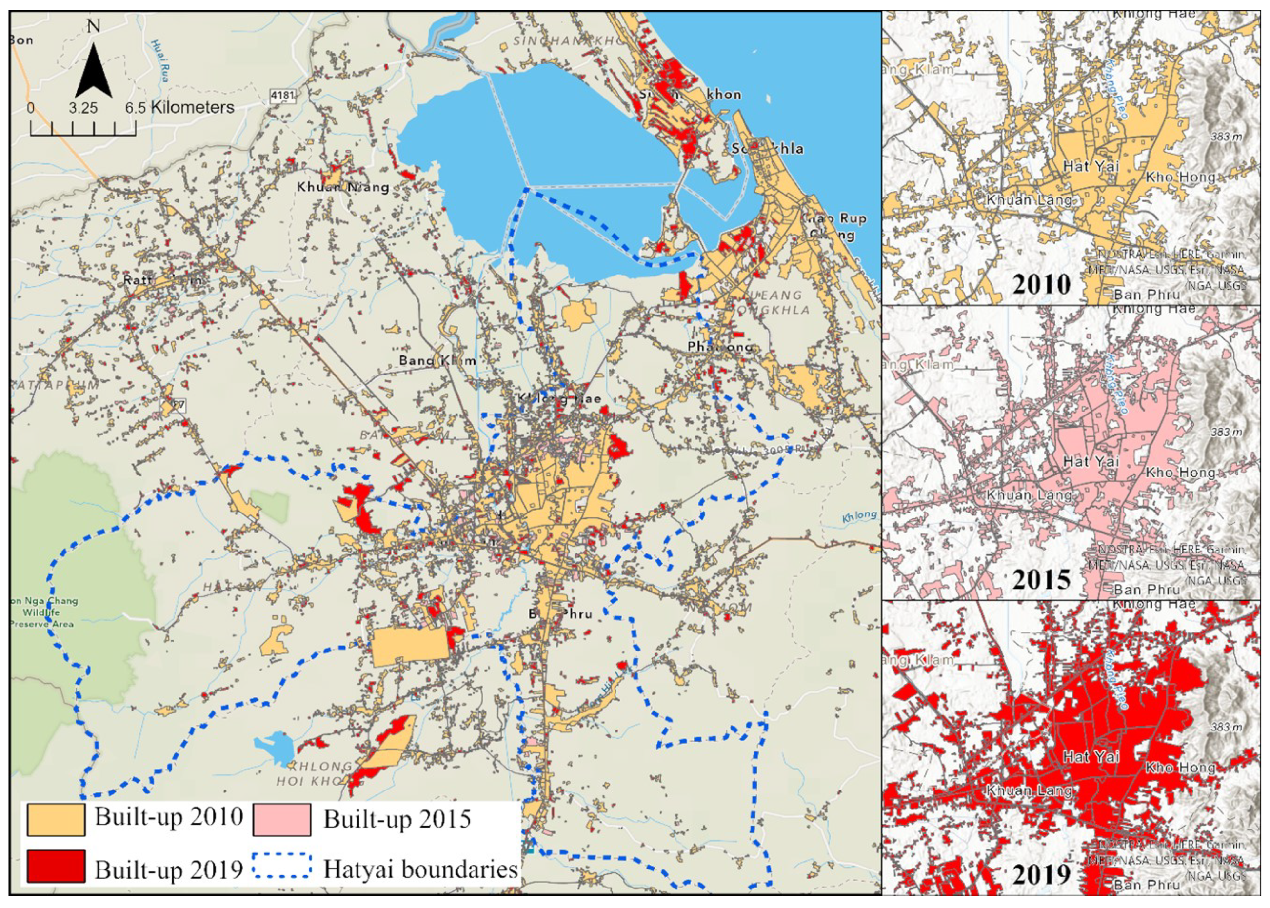
As shown in Figure 1, between 2010 and 2019, low- and medium-density residential areas and rural agricultural areas in Hat Yai City experienced urbanization with the construction of infrastructure such as roads and houses. The construction of this infrastructure proceeded without strict enforcement of urban planning laws, which reduced the water intake area due to land reclamation and surface concrete, which had a significant impact on water runoff during the rainy season [1].

The reduction in natural water intake areas has resulted in frequent flooding problems. Frequent flooding areas (red pins) are recorded by the Hat Yai municipality and identified from the analysis of satellite imagery. Figure 2a shows the pattern of flooding in Hat Yai. The Khlong U-Tapao Basin (black arrow) in Sadao District flows through Hat Yai City and drains into the Songkhla Lake within 10–30 h, causing the U-Tapao Canal to overflow. Rainfall of more than 100 mm in 6 h causes runoff from Khohong Hill (brown arrow) into the Khlongrien Basin [2]. Repeatedly flooded areas are also shown in Figure 2a. Damage caused by flood has been huge. For example, the flood event in 1988 caused damage of more than THB 2000 million, while 12 years later in 2000, flooding caused damages of THB 10 billion and the deaths of 30 people.

After this flood, the government upgraded the U-Tapao Canal by constructing natural branch drainage canals [3]. However, the fact that a major flood in 2010 impacted 80% of the area shows that these structural improvements to the drainage of the area did not reduce economic losses and social risks. Data analysis from field surveys [4], showed that many roads were cut off by the flood, as shown in Figure 2b. A maximum flood level of 4 m was recorded, with damage estimated at more than THB 16 billion. Therefore, in addition to upgrading the canal, flood countermeasures such as ensuring of evacuation routes need to be adequately carried out by meeting about the situation before, during, and after flood events.

The objective is to evaluate the road network and suggest alternate routes during flood disasters using a dynamic traffic assignment (DTA) model to reduce loss of life and manage evacuation measures. Subsequently, the secondary objective of this study is to estimate evacuation time and identify measures to control flooding based on past evaluations.

This paper is organized as follows. First, the background and objectives of the study are explained in the introduction. Second, the literature on the identification of flooding evacuation procedures and dynamic traffic assignment (DTA) is reviewed. Third, the summary of background information, such as flooding impact on road transportation and actual evacuation behavior in Hat Yai, is described. Fourth, the DTA model network by Dynameq is explained. Fifth, the result of the scenario analysis is analyzed and evaluated based on the travel speed, VHT, and VKT. Finally, conclusions and possibilities for future work are summarized.

2. Literature Review

Planning an evacuation is the best way to avoid or mitigate the effects of disasters such as hurricanes [5,6,7,8], nuclear power plant accidents [9,10,11], and earthquakes [12,13,14]. Several previous studies have also been conducted to identify flooding evacuation procedures and instigate optimal preventive measures [15,16,17,18,19,20]. Evacuation success depends on adequate warning time, public preparedness, clear instructions, evacuation routes, traffic conditions, and dynamic traffic management measures [19,20]. In particular, findings showed that the key elements influencing the efficiency of evacuation services included controlling road conditions at the outgoing motorway connections in the given network during the evacuation period and access capacity from the downtown area to outbound freeway links. A thorough analysis of the traffic impacts of a mass evacuation of the Halifax Peninsula under several flooding scenarios was also conducted [21]. However, variables such as human behavior and the type of disaster that triggers the evacuation are uncertainties [22].

In an evacuation scenario, extremely concentrated time-varying origin–destination (O-D) demands result in highly unstable and disorderly link flows, with oversaturated queues. In practice, the methodology generally followed by evacuation studies is to assume the percentage of the population that is going to evacuate and then use behavioral response curves to estimate the timing of the evacuation under random population distributions [23,24] with demand based on linearized S-curves at half-hour intervals related to a clearance time lower in magnitude than the average travel time. The clearance time may be insufficient to provide adequate planning measures unless comprehensively analyzed. Evacuation response problems can also be solved using census demographic data and travel survey data to calculate the proportion of the population commuting into, out of, or across an at-risk area to generate the percentage of the population that is going to evacuate and make predictions on the behavioral capabilities of the different social groups [25]. To prevent traffic congestion, staggered departure times could be assigned to different groups of evacuees in endangered areas [26,27]. Evacuation overcrowding on the roadways will result in a partial or full loss of capacity at certain network links [24,28,29,30,31] because it affects reliable evacuation times under realistic transportation network conditions.

An evacuation planning model aims to achieve different network optimal states that mirror real-world evacuation events. The network might lose capacity as a result of both human and disaster-related factors, while variations in the size and timing of evacuation demand generated by the dynamic traffic assignment (DTA) model will provide more realistic outcomes. DTA has been used to determine evacuation scenarios in macroscopic [32,33,34], mesoscopic [35,36,37,38], and microscopic models [39,40,41,42,43,44].

The viability of using the Dynasmart-P DTA model was assessed for alternate traffic evacuation tactics in downtown Minneapolis, Minnesota in the event of an emergency requiring the evacuation of a sold-out crowd from the Metrodome [45].

Several previous studies were conducted to identify flooding evacuation procedures and instigate optimal preventive measures. Land surface modeling connecting the Halifax Stream and transportation networks was used to determine the magnitude of the flood and associated network disruption. An examination of network performance showed persistent congestion of 4 to 7 h during the evacuation. An analysis of transportation systems in emergency conditions due to disaster scenarios was also presented in Di Gangi (2009)  [46]. Piyapong et al. (2021) used mesoscopic (DTA) as a tool to improve road network traffic flow performance under different flood conditions by applying the concept of the Macro Fundamental Diagram (MFD) and take appropriate traffic control measures. A mesoscopic (DTA) model was developed to determine quantitative indicators for estimating the exposure component of total risk incurred by road networks [47]. Appropriate quantitative methodologies based on a dynamic approach (DA) are a useful tool to support evacuation strategic planning at different regional scales. A DA concept to simulate the supply of transportation and the interplay between supply and demand for travel in an urban road transportation system under emergency circumstances was presented [48]. Traffic data were collected during a practical evacuation experiment carried out at Melito di Porto Salvo, Italy and used to calibrate and validate transport supply models. A calibrated DA model can be a helpful tool when planning and managing road networks and transportation in emergency situations. A modeling approach was conducted on the Boston, Massachusetts road network and a range of practical challenges related to evacuation modeling was examined in Balakrishna et al. (2008) [49].

There is a case study used DynaMIT, a cutting-edge DTA model, to demonstrate the advantages of network management methods. A Cellular Automata-based Dynamic Route Optimization (CADRO) method was also considered for hydrodynamics, terrain, and human response time to determine dynamic flood evacuation routes (FERs) [50]. The CADRO method was employed in a suburb of Yangzhou City, China. Findings showed that compared to the conventional method used for evacuation route optimization, average and max lengths of FERs were reduced by roughly 32.70%, 34.04%, and 7.90%, respectively. Mathematical model formulations underlying traffic simulation models used in evacuation studies and behavioral assumptions were assessed by Pel, Bliemer, and Hoogendoorn (2012) [51].

Evacuation travel behavior, which is based on the viewpoint from the social sciences, as well as empirical investigations have also been discussed in detail. Traveler decisions, such as whether to evacuate, what time to leave, where to go, and how to get there, can be forecasted using simulations. Facets of transportation systems under emergency circumstances brought on by dangerous events were examined by Di Gangi (2011) [52] using a mesoscopic (DTA) model to produce objective measurements and assess the exposure attributes of overall risk suffered by regional road networks. Impacts on the transport network were examined to demonstrate how effective quantitative approaches built on a DA concept were a helpful tool to aid evacuation strategic planning. A macroscopic traffic flow model utilizing a DYNEV II large-scale evacuating planning system was presented by Lieberman and Xin (2012) [34]. This concept was represented as a single processing unit for generalized networks with connection lengths ranging from 100 feet to several miles. The model allowed simulation time steps of one minute or longer, significantly greater than utilized for other models, and supported up to four turn motions from each link with a wide variety of traffic controls at junctions to accurately reflect congested areas and their spill back processes.

Therefore, this study creates a novel model to determine the effect on flood evacuation time estimation of varying water depth with evacuation behaviors. Generally practical, the methodology followed by evacuation studies is to assume the percentage of the population that is going to evacuate. Then, it uses behavioral response curves to estimate the timing of the evacuation under random population distributions [23,24] with demand based on linearized S-curves at half-hour intervals related to a clearance time lower in magnitude than the average travel time. The clearance time may be insufficient to provide adequate planning measures unless comprehensively analyzed. However, this study fills the gap by using the data from the questionnaire survey on flood evacuation behavior in Hat Yai Municipality to analyze evacuation behavior during the flood. Moreover, this study considers the efficiency of the road network, which decreases with rising water levels, leading to the ability to estimate evacuation time. This can be determined from the inundation model characterizing the inundation in the study area. The model used in this study brings the advantage from both macroscopic and microscopic levels, called the mesoscopic level, which is a novel application for solving the road traffic network that increases the modeling accuracy compared to the macroscopic without the need to prepare the same in-depth details as on the microscopic level. The expectation is to obtain the preparation plan, which is a solution helping government officials to avoid evacuation delays and loss of life and property.

3. Background Information

Travel models can analyze evacuation processes and estimate evacuation times. However, simulation is a time-consuming process that includes model development, validation of data collection, model testing, and data interpretation. In this study, the authors updated the existing traffic demand by using a static origin–destination (OD) matrix to describe the trip distribution. The estimation was based on current traffic counts using matrix algorithms, which have been available for many years for static assignment models and can be used to pre-process demand matrices for dynamic traffic assignment (DTA) models. Trips were assigned to the city’s traffic analysis zones and existing roadway networks extracted from the model. Reference trip tables were constructed for areas outside the city to form background vehicle traffic as trips traveling to or from evacuation zones. Data were taken directly from the travel model for a typical day and then distributed over each hour of the day. The DTA model only reflected personal vehicle traffic, with travel modes such as public transit or walking not considered. The overall vehicle travel demand was based on hourly typical travel daily activity until the evacuation notice was given. The travel demand for evacuation zones was separated from background traffic not associated with evacuation zones. Departure times for leaving the evacuation zones varied according to the time and type of the event. To conduct this study, the existing traffic demand was updated as a static origin–destination (OD) matrix. Flood evacuation behavior in each area was reviewed including percentages of evacuation timing (do not evacuate immediately after warning or based on flood level), evacuation destination (out zone, evacuation center), and travel patterns used for evacuation (walking, passenger car, motorcycle). These variables are important to estimate the OD matrix of each flood scenario in a particular area.

3.1. Network Configuration and Parameter Setting

Estimating the spatial and temporal distribution of travel demand is important for DTA models. One common approach is to use the calibrated OD matrix of macroscopic travel demand models as Static Traffic Assignment (STA). This study used the OD matrix from the regional demand model of Hat Yai District developed by Luathep et al. (2013) [53] using the EMME program. The road network of Hat Yai City consists of 2507 links and 923 nodes including 142 zone centroids. Among the nodes, 41 are intersections with a traffic signal, as shown in Figure 2c. Connectors were used to link the zone centroids to the network. These were carefully placed to be as reflective of the actual situation as possible while avoiding false network congestion.

The regional demand model data were then imported into the Dynameq program, and a DTA road network was set up. Signalized intersections and signal plans and timings were imported from the real world. The following settings correspond to Dynameq settings required to run the assignment. This was implemented in order to get reasonable paths while still respecting the observed free-flow times on locals and collectors. Dynameq allows for signal offsets as inputs and provides improved computational efficiency compared to a microscopic model in a regional network. This is particularly important for simulation-based DTA. All movement capacities were calculated based on their types and parameters, such as gap acceptance and property relationships. At intersections, movements and rules were based on the signal plans. Links in the modeled network, characteristics of network geometry including position, shape, and length, and functional characteristics such as free-flow speed correspond to the real-world existing road network. Link capacity was calculated using three factors: link free-flow speed, effective vehicle length, and vehicle reaction time.

There is the possibility to clear the traffic during the flood by controlling the traffic signals using a detecting system, which gives an input to the current system, with the goal that it can adjust the changing traffic density patterns and provides a vital sign to the controller in a continuous activity. Using this method, improvement of the traffic signal switching expands the street limit, saves time for traveling, and prevents traffic congestion.

As mentioned above, model parameters such as drivers’ response time and vehicle relative length can vary. Here, 6.25 m and 1.25 s were chosen as the worldwide effective vehicle length and response time parameters, respectively. In Dynameq there are default values for passenger car average effective length (6.25 m) and average response time (1.25 s). The default and user-specified effective length and response time values can also be altered for entire scenarios or for individual links through the use of multiplier factors for Effective Length and Response Time. Any modifications to these two parameters resulted in a change in jam density and maximum flow rate at each link. The free-flow speed is also an important component that defines link capacity.

3.2. Origin–Destination Matrix

Data to produce the DTA model were obtained from the Hat Yai regional demand model. This static assignment model could be reused for long periods and was also used as a pre-processed travel demand matrix for the DTA model. Static traffic demand was designed using a conventional 4-step model. Trip distribution was divided into two groups as aggregate (secondary data) and disaggregate (survey) methods. Both models were also combined as mixed distribution models [54]. A trip distribution model can be estimated using a Poisson regression using variables extracted from a trip generation model [55], with no constraints on the spatial relationships between origins or destinations, thereby guaranteeing good reliability of the estimated parameters [56]. The cost objective, referred to as an entropy function, plays a key role in terms of potential, exponential, and combined trip distribution and is most commonly used to describe the empirical relationships between economic and behavioral variables [57]. For this study, with extracted trip production and trip attraction from the Hat Yai regional model for every zone in the network, we then used the growth rate of the population [58] to calculate the production and attraction trip of 2022. The calculation of the entropy function between each OD pair d, $E_d$ in the network is defined as

$$E_d=exp\left(-\frac{u_{od}}{\overline{u}}\right)$$

(1)

where

$u_{od}$ is the free-flow speed travel time between OD pair d;

$\overline{u}$ is the mean of free-flow travel time between all OD pairs.

The process of trip distribution to find the prior OD matrix, the matrix balancing method [59], was used, which balances the matrix of trip production data and attraction data by entropy as weight for distribution. The prior matrix from the previous one will be calibrated based on the observed hourly link volume. Using this method, the travel demand matrix was automatically adjusted to existing peak-hour traffic volume. This model was also used as a gradient method [60] to minimize the objective function as a measure of the distance between observed flows ($v_a^{\prime }$) and assigned flows $v\left(g\right)$. This distance was weighted by the constant $\alpha ,(0\le \alpha \le 1)$, which was used to weigh deviations from the counts, the sum of squares between the new matrix, and also the difference between the adjusted matrix g and the original matrix to be adjusted g’, as a constant used to weigh deviations from the adjusted and the original matrices [61].

The mathematical formulation is shown in Equation (2).

$$\mathrm{Minimize}:z(v,g)=\alpha \sum _{a\ni A}{(v_a\left(g\right)-v_a^{\prime })}^2+(1-\alpha )\sum _{i\ni I}{(g_i-g_i^{\prime })}^2$$

(2)

where

$a\in A$ are the links that have counts;

$v\left(g\right)$ is the assigned flow using the adjusted matrix;

$(1-\alpha )$ is used to weigh the deviations from the adjusted and the original matrices, and OD pairs are denoted by the index $i,i\in I$;

I is the OD cells that are included in the demand term of the objective function.

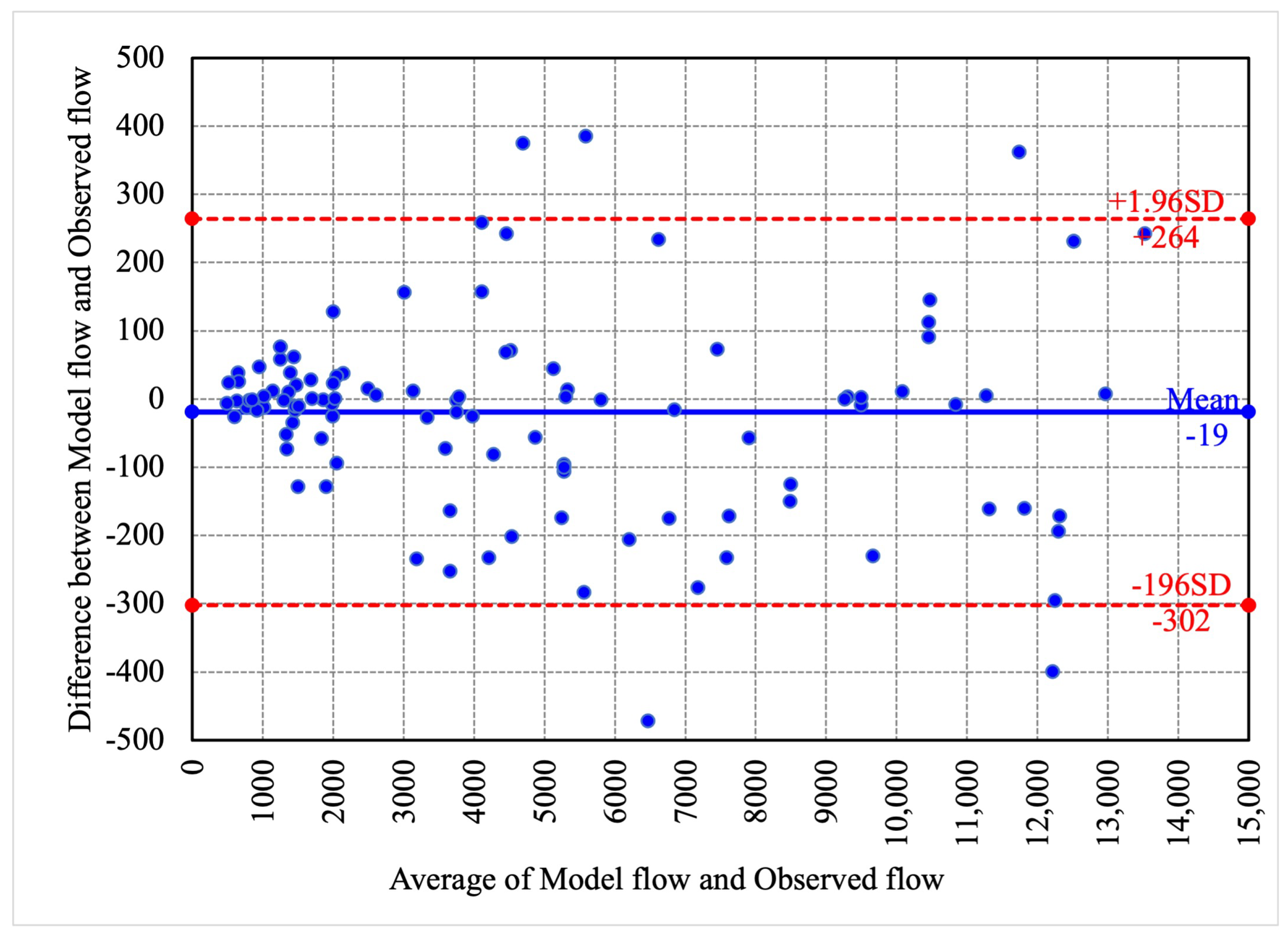
The best value choice as parameter $\alpha$ is dependent on the data when a particular adjustment is carried out, such as the number of links with counts. The higher the value of $\alpha$, the more weight is given to fitting the counts. To preserve the structure of the adjusted matrix, a judicial value of $\alpha$ would give weight to the demand matrix deviations. The model was calibrated using a set of 1-morning peak hour of traffic counts and included data from annual average daily traffic (AADT) converted to peak hour by comparing the percentage of 1 peak hour with daily traffic. Peak-hour morning traffic was used for calibration because the distribution of traffic was more uniform than in the afternoon, as seen from the Peak Hour Factor (PHF). The 110 traffic links were compared with the model and results were assessed using Bland–Altman plots, as shown in Figure 3.

Figure 3 is the plot of differences between model flow and observed flow vs. the average of the two measurements, which help to investigate any possible relationship between measurement error and the true value. Results show a bias of 19 units, represented by the gap between the X-axis, corresponding to zero differences, and the parallel line to the X-axis at 19 units. After ensuring that our differences are normally distributed, we can use the standard deviation (SD = 144) to define the limits of agreement at a 95% confidence interval. So, results measured by model flow are approximately 305 units below or 264 above observed flow (red line).

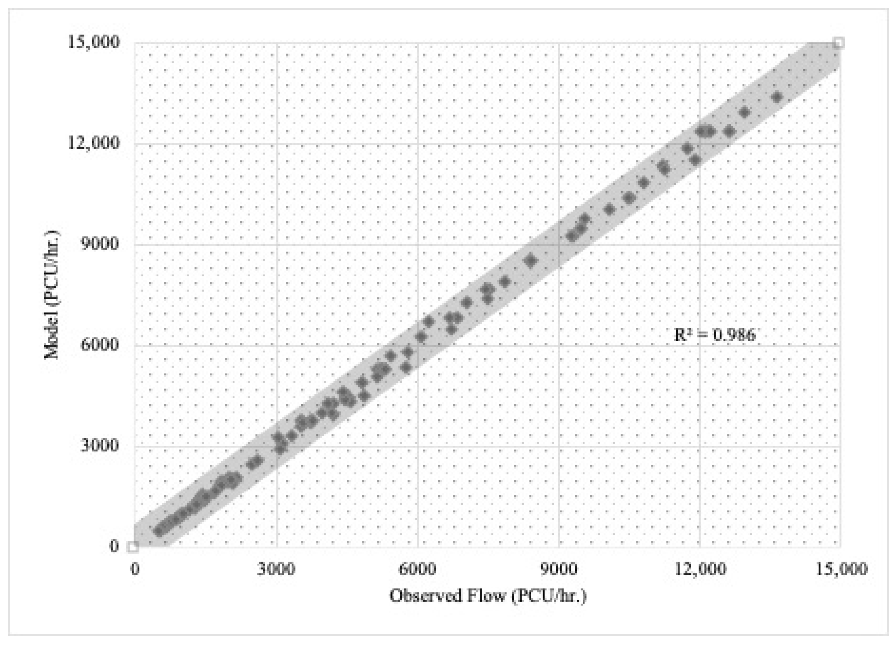
Then, considering the statistical values by using a two-sample t-test between model flow and observed flow, the results are as follows. The mean in the model flow group was 4896.945 (SD = 3804.629), whereas the mean in the observed flow was 4878.239 (SD = 3793.905). A two-sample t-test showed that the difference was not statistically significant at the t-test statistic value, where p-value = 0.971 > 0.05 (95 percent confidence). The degree of correlation was determined after traffic demand was adjusted by the iteration process. The degree of correlation was calculated between the manually counted traffic volume and the developed model traffic volume. Results showed that the developed model was calibrated at 0.986, as shown in Figure 4.

3.3. Evacuation Behavior during the Flood

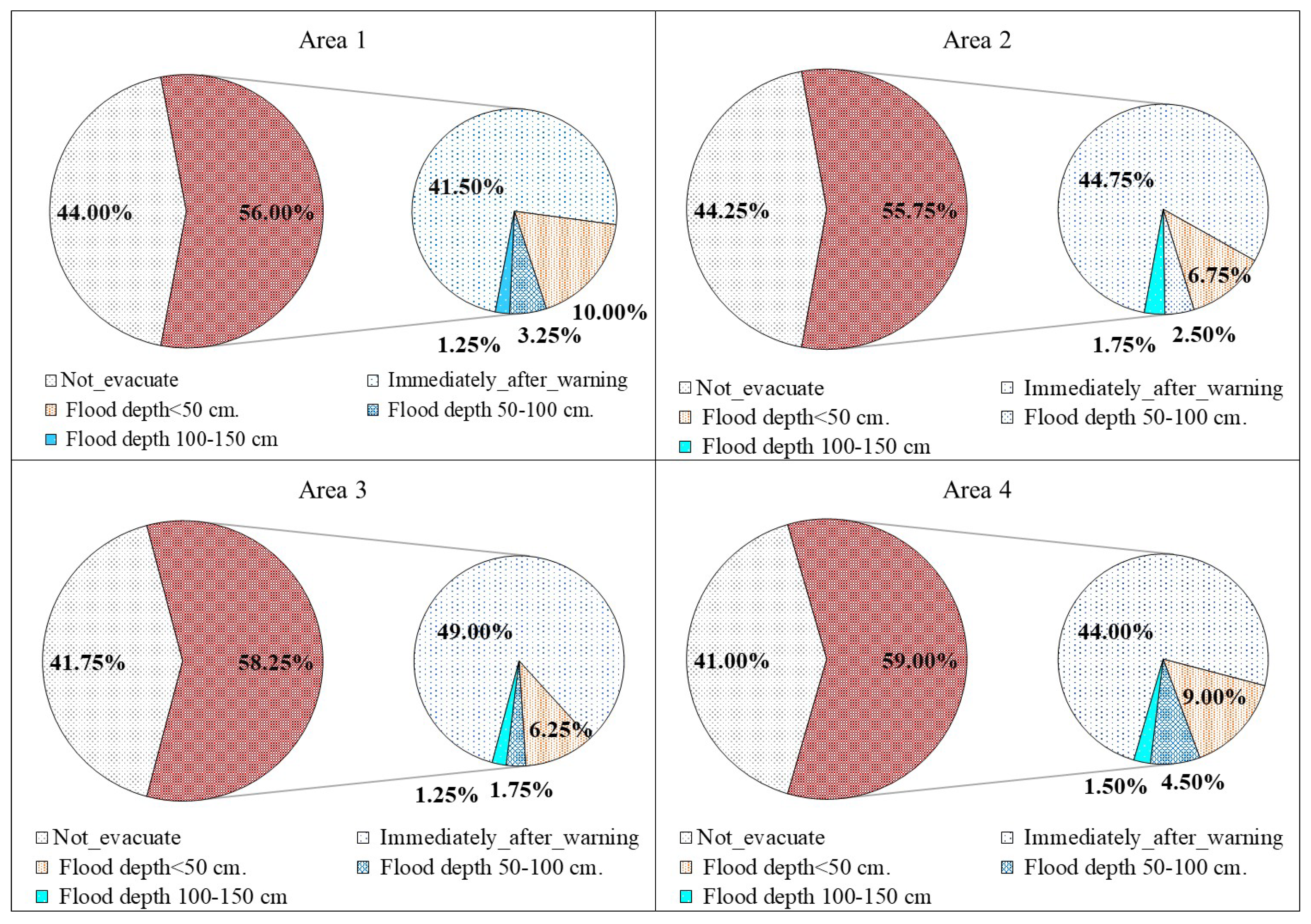
Travel and evacuation behavior data collected from a questionnaire were used to investigate people’s behavior before, during, and after a flood incident from past experiences. A total of 102 affected communities (zones) were integrated into four main areas (zone groups) according to the Hat Yai flood response [62] to determine the proportions of different evacuation decisions during flooding, as shown in Figure 5. More people in all four areas of Hat Yai decided to evacuate than decided not to evacuate. Evacuation scenarios were evaluated immediately after the warning: water level less than 50 cm, water level of 50–100 cm, and water level of 100–150 cm.

The secondary data in

Table 1. Data from the questionnaire on flood evacuation behavior in Hat Yai Municipality.

Area	Destination(%)		Transport Mode Choice (%)
	Evacuation Center	Outzone	Walking	Passenger Care	Public Transport
1	74.60	25.40	11.11	87.98	0.91
2	67.00	33.00	9.00	90.00	1.00
3	71.60	28.40	8.20	90.40	1.40
4	70.74	29.26	11.80	86.60	1.60
Average	71.00	29.00	10.02	88.75	1.23

Source: kb.psu.ac.th/psukb/handle/2016/11582 (accessed on 29 May 2022).

were examined to determine the evacuation behavior of people in Hat Yai municipality. Results showed that, on average, 71% of people chose to go to evacuation centers provided by the local government within each flooded area, with 29% going to centers outside the flooded areas. For evacuation, 88.75% of people chose private cars as the primary mode of transport.

For sudden flood situations, this study applied the calibrated static OD matrix as a 1 h peak to evaluate an evacuation plan. This plan was then analyzed to determine the proportion of evacuation decisions during flooding with water levels less than 50 cm and then consider the trip production of zones distributed to trip attractions as evacuation zones designated by the local government. Private cars were selected as the main mode of transport for evacuation, as shown in Table 1. Cars could drive through flooded roads with water levels less than 50 cm and were assigned based on reduced road efficiency according to flood depth.

3.4. Flooding Impact on Road Transport

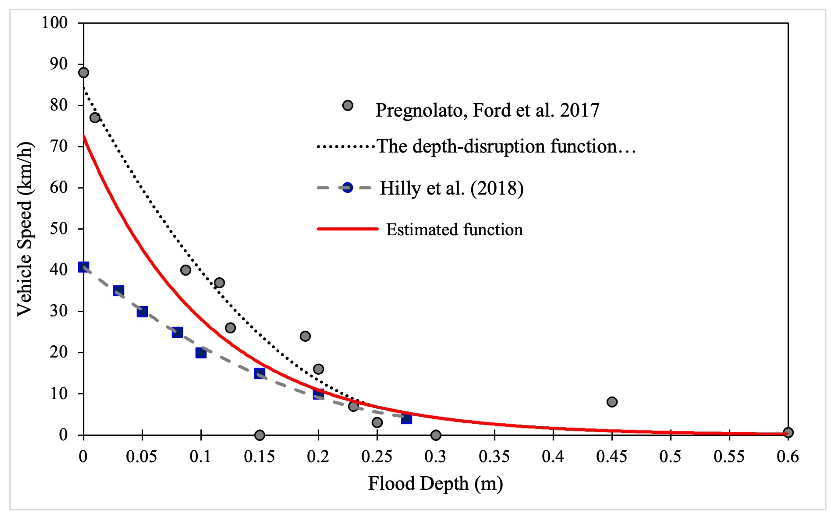
Flood levels have different effects on the safety and reliability of the road network. Several studies examined flooding effects on vehicle speed [63,64,65,66,67,68,69,70,71,72,73,74,75,76,77,78]. Pregnolato, Ford et al. [79] combined data from experimental studies, observations, and modeling to develop a function that described speed limits of different vehicle types based on their dimensions (small vehicles, large vehicles, and heavy vehicles). Interviews with taxi drivers and pickup truck drivers also showed a relationship between flood depth and vehicle speed as a curve trend (orange line) and combined data from experimental studies, observations, and modeling to develop a function that described speed limits of different vehicle types based on their dimensions (small vehicles, large vehicles, and heavy vehicles). Interviews with taxi drivers and pickup truck drivers also showed a relationship between flood depth and vehicle speed [80] as a curve trend (estimated function), as shown in Figure 6. For this study, we change the free-flow speed parameter on the link to the set value according to the results obtained by the flood function at different levels. However, we consider a flood depth not exceeding 30 cm, in which the vehicles’ speed is reduced to 0 km/h as the ultimate level for safe driving of most vehicles. At a flood depth of 30 cm, vehicle speed is reduced to 0 km/h. When driving through flood water of less than 30 cm depth, drivers should consider safety as their main priority. Driving in a water level of 5–10 cm is considered safe because the water can easily be seen on the road surface. A water level of 10–20 cm is also considered safe for cars to pass normally, but it may impact the movement of smaller cars with lower ground clearance. Most passenger cars have a height clearance of 150–170 cm, and water at a 20–30 cm depth will cover the exhaust pipe outlet. Short distances are manageable, but traveling long distances is not recommended for safe driving. Water levels above 30 cm are considered dangerous for all types of vehicles, and driving is not recommended.

4. DTA Model Network

This study presented the DTA at the mesoscopic scale using Dynameq 4 to efficiently model traffic lane usage. Traffic flow is described with three components: car following, gap acceptance, and lane changing [81]. Following the above, the application of the relationships between flood depth and vehicle speed, which define vehicle motion on the roadway through time of the car-following model, is shown in Equation (3).

$$x\left(t\right)=MIN\left[\left(x_f(t-RT)+FFS\times RT\right),\left(x_l(t-R)-EL\right)\right]$$

(3)

where

$x_f$ is the location of the following vehicle at time t;

$x_l$ is the location of the primary vehicle at time t;

$FFS$ is the free speed of the roadway (km/h).

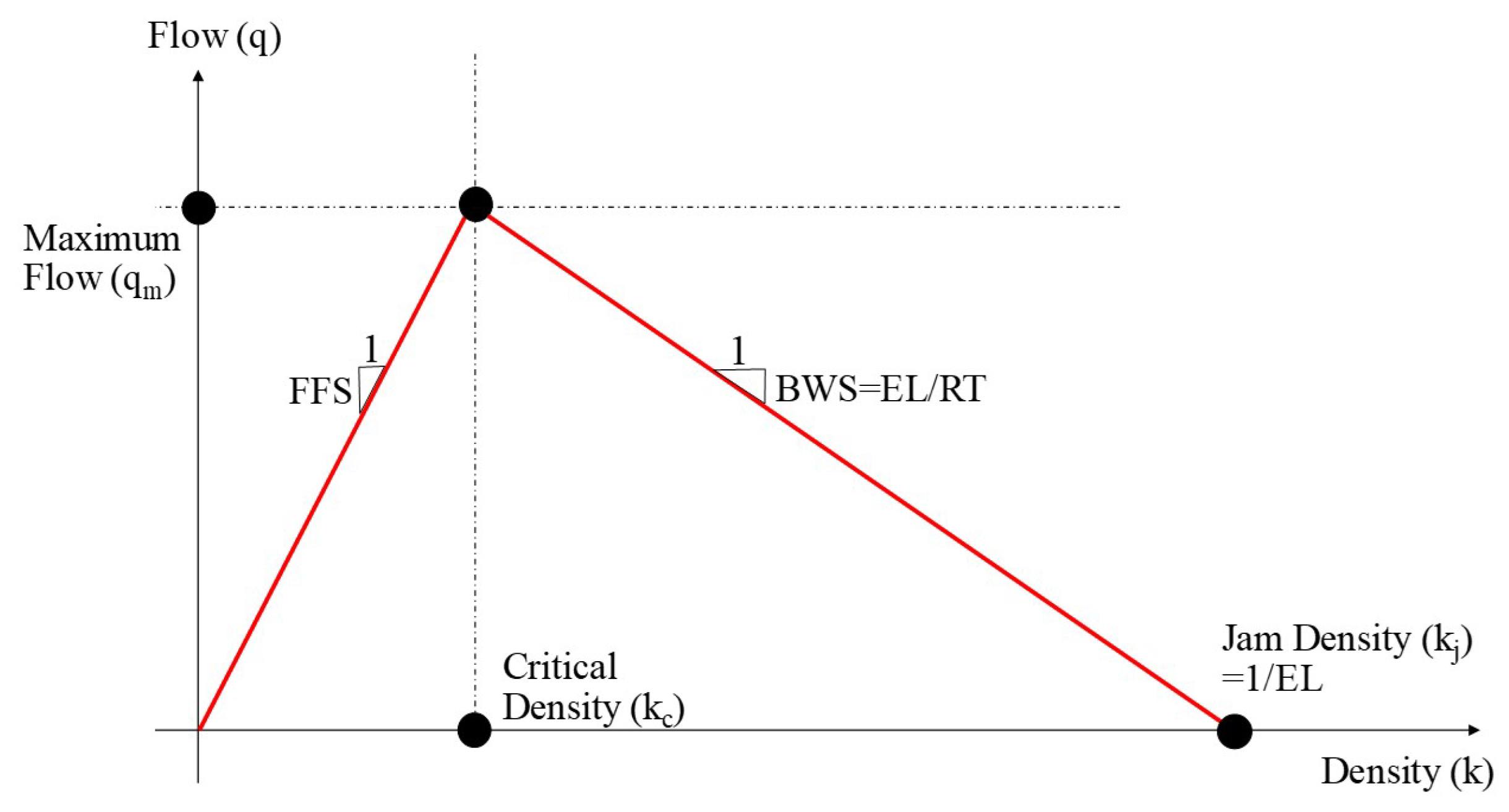
Equation (3) describes the trajectory of a vehicle based on a triangular diagram, as shown in Figure 7, defined by the three parameters of free-flow speed ($FFS$), maximum flow ($qm$), and jam density ($kj$), which represent flow as a function of density in each link. This is similar to how Newell’s kinematic wave theory [82] was used for the propagation of traffic delay. A positive slope in the first segment (increase, $k<kc$) indicates a vehicle moving at $FFS$, where the absolute value of the negative slope in the second segment (decrease, $k>kc$) is equal to the backward wave speed ($BWS$).

This fundamental diagram shape changes if the average vehicle speed is reduced as a result of any condition, such as bad weather affecting the maximum flow that can traverse a road segment. The Dynameq program used a triangular shape diagram to describe only three macroscopic traffic flow parameters (maximum flow, jam density, and wave speed), thereby reducing the required input data. Values of the three macro traffic flow parameters for a specific vehicle type and a specific road were determined from the free speed of the link, the effective length, and the response time of the vehicle type, as shown in Equation (4) below.

$$q_m=\frac{1}{(RL+\frac{EL}{FFS})},k_j=\frac{1}{EL},v_{wave}=\frac{EL}{RL}$$

(4)

where

$q_m$ is the maximal possible flow rate (veh/h/lane);

$k_j$ is the stationary state when traffic flow stops completely, or jam density (veh/km/lane);

$v_{wave}$ is the speed at which shock waves move through a platoon of traffic against the direction of flow for a specific vehicle type (km/h);

$EL$ is the average space that the vehicle occupies on the road;

$RL$ is the driver response time to change speed when the traffic flow state ahead changes and the backward wave speed ($BWS$) is the rate of propagation of the change in traffic flow state upstream as a result of changes in the downstream traffic flow.

At DTA equilibrium, vehicles starting their trips in the same zone and ending their trips at the same destination will have the same travel time. To reduce travel time, the dynamic user equilibrium (DUE) model was used [83]. This is a time-dependent path flow that uses the method of successive averages (MSA). Corresponding path travel times were determined following the method of Mahut et al. 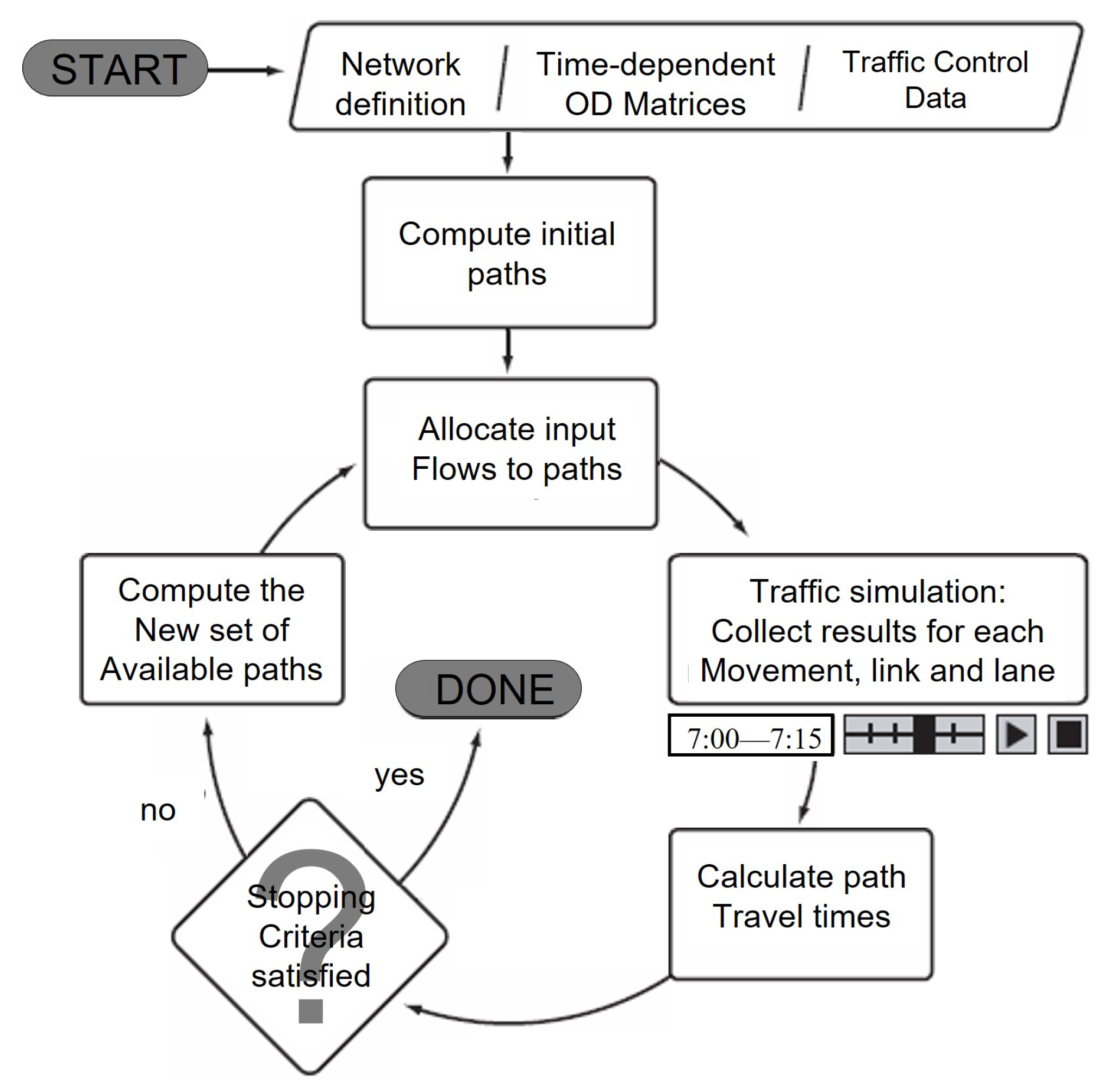(2004) [84] using the Dynameq 4 program. The overall structure of the study is presented as a schematic algorithm in Figure 8.

This study used two major components. The first determined the latest set of time-dependent paths using the last cycle time-dependent paths, while the second defined the actual travel time after completion of a given set of path flow rates. Large numbers of vehicles in each particular zone caused network loading problems. To solve this, a route-based dynamic traffic model was adopted. The initial paths must be provided to start the algorithm; to satisfy this, the shortest paths are used based on the free-flow circumstances. The mathematical equation representing dynamic equilibrium, consisting of demand for the OD pair $I\left(g_i^a\right)$, path flow for path $k(h_k^{(a,n)})$, travel time for path $k(s_k^{(a,n)})$, and the shortest travel time for the OD pair $I(u_i^{(a,n)})$, was calculated for every time interval during the assignment (a) for all iterations made during the simulation (n). The procedure is shown below (Algorithm 1).

Algorithm 1 Dynamic MSA Equilibration Algorithm [85,86,87,88]
Step 0	Initialization (iteration $n=1$); compute dynamic shortest paths based on free-flow travel times and load the demands to obtain an initial solution; $n=n+1$
Step 1	If $n\le N$, compute a new dynamic shortest path and input path flow ($h_k^{(a,n)}$) to each path $k\in K$
	$$h_k^{a,n}=\frac{g_i^a}{n},i=1,2,\dots ,\left|i\right|$$
	If $n>N$, identify the shortest among used paths and redistribute the flows as follows:
	$$h_k^{a,n}=\left\{\begin{array}{cc}{h}_k^{a,n-1}\left(\frac{n-1}{n}\right)+\frac{g_i^a}{l}\hfill & \mathrm{if}{s}_k^{a,n};k\ni K,i\ni I,\mathrm{all}a\hfill \\ h_k^{a,n-1}\left(\frac{n-1}{n}\right)\hfill & \mathrm{otherwise}\hfill \end{array}\right.$$
Step 2	If $N\le L$ as the maximum number of iterations or $RGap\le \epsilon$ as maximum average relative gap, STOP; otherwise, return to step 1

Figure 8 illustrates the two main components of the Dynameq system, namely the route choice model and the dynamic road traffic network loading. The system uses an iterative approach to achieve dynamic user balance for dynamic traffic assignment (DTA) based on mesoscopic traffic simulation. In each iteration, the route choice model and the dynamic network loading model are run. The route choice model first allocates the OD traffic volume of each point in the road traffic demand OD matrix at each departure time to the effective road network based on the existing road traffic conditions. Subsequently, the traffic flow of the road section that changes with time is transferred to the traffic simulation model. This calculates the dynamic travel time of the road section, which is then sent to the route choice model to correct the next route choice. This iterative process continues until a predetermined critical value is reached, indicating equilibrium in the system. Overall, the Dynameq system provides a robust and efficient approach for simulating and analyzing dynamic traffic patterns under various scenarios [81].

A comparative gap is used in DTA to signify a perfect DUE flow. The stopping criterion of the MSA was defined using the gap function, as shown by Equation (5) [88].

$$RGa{p}^{a,n}=\frac{{\sum }_{i\in I}{\sum }_{k\in K}{h}_k^{a,n}{s}_k^{a,n}-{\sum }_{i\in I}{g}_i^{a,n}{u}_i^{a,n}}{{\sum }_{i\in I}{g}_i^a{u}_i^{a,n}}$$

(5)

where

I is the set of all OD pairs;

$K_i^a$ is the set of paths for the OD pair i and assignment interval $a$;

$h_k^{a,n}$ is the path flow for path k in interval $a$ in iteration n;

$g_i^a$ is the OD demand for OD pair i in interval $a$;

$s_k^{a,n}$ is the travel time for path k in interval $a$ in iteration n;

$u_i^{a,n}$ is the shortest travel time for OD pair i in interval $a$ in iteration n.

5. Results

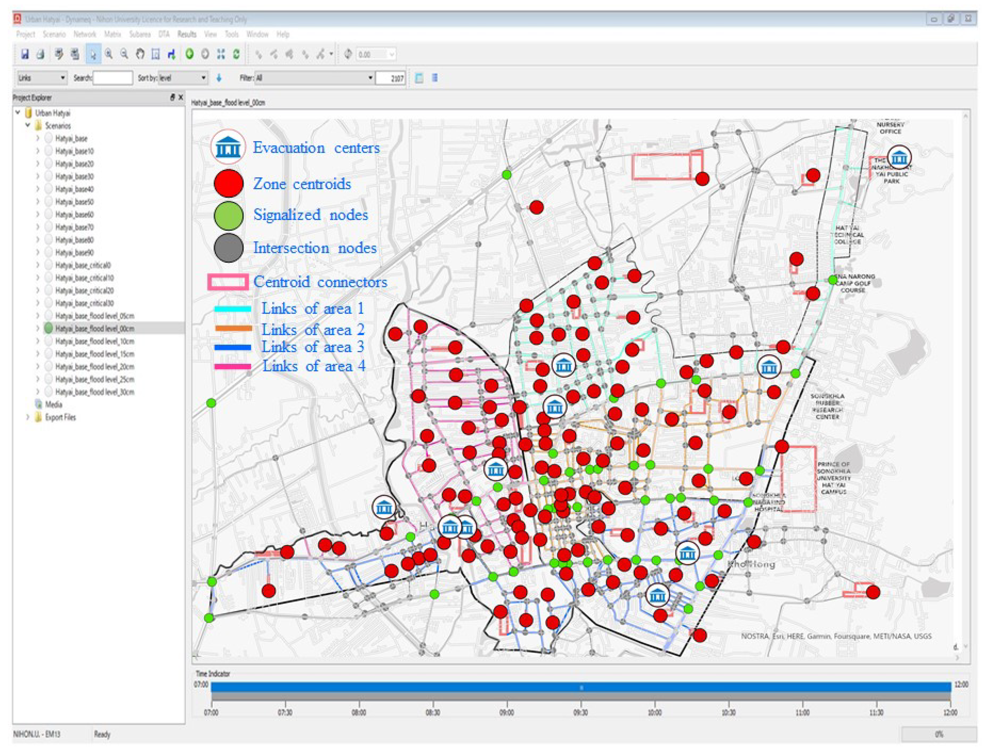
This study was performed by adjusting the free-flow speed factors of the model. Alternative scenarios were developed based on evacuation demand (Flood ≤ 50) in Figure 6 and FFS according to flood depth and vehicle speed in Figure 7. In the first baseline scenario, the calibrated model identified potential congestion locations throughout the network. This situation was utilized as the baseline to compare other situations including flood depths of 0–5, 5–10, 10–15, 15–20, and 20–30 cm. The mesoscopic traffic network model for Hat Yai developed by the Dynameq 4 platform is shown in Figure 9.

There were 142 zones including 133 communities and 9 evacuation centers, 923 nodes, 2507 links, and 41 signals. The appropriate OD matrix of personal vehicles, estimated using the EMME subarea tool, was included in the imported demand matrices from the Hat Yai regional model. A simulation was conducted, without a traffic volume warm-up interval, to load the network at the beginning of the analysis period and cool down for network clearance. The authors selected a ten-minute assignment period. This was identical to 6 cycles for a 1 h allocated OD matrix. Up to 20 routes were searched for one assignment interval. Stop conditions were set at 200 cycles with a comparative difference of 1%.

5.1. Result of Model Convergence

There is consistency with previous research on short-notice evacuation events, as documented in the Approach to Modeling Demand and Supply for a Short-Notice Evacuation [89]. Departure time from the evacuation zones varies according to the flood levels, with residents in the greatest danger evacuated first followed by those closer to the highway. For events where ample notice is given, less time is required to prepare for the evacuation. The time required to prepare for an evacuation is typically longer, as residents need to pack their belongings and collect their animals. Using different evacuation starting times will lessen the impact of the evacuation on roadway conditions. The evacuation curve can be shifted or compressed toward the end of the assumed evacuation event. When considering evacuation orders, public officials must allow the residents ample preparation time for departure balanced against the dangers of delaying the evacuation. Integrating travel demand modeling and flood hazard risk analysis for evacuation and sheltering should ensure the redundancy of critical transportation routes and allow continued access and movement in the event of an emergency. This may also include addressing vulnerabilities of bridges, major roadways and highways, railways, traffic signals/traffic control centers, and other transportation facilities and infrastructure components to ensure the availability of multiple viable evacuation routes [90,91].

Considering the implemented transportation operational strategies for evacuation events, in the assessment above, capacities are based on typical limiting signal green time allocations. The development of an evacuation coordination plan would achieve additional capacity. Traffic signals in vulnerable areas could be prioritized, with improvements connected online to the Traffic Management Center together with contingency plans for loss of power and communications grids [92].

Before investigating the impact of floods on the road network, this study first assessed the sensitivity of the network’s performance to degradation in free-flow speed under dry conditions. This was carried out by considering scenarios in which the free-flow speed was reduced by 10%, 20%, 30%, 40%, 50%, 60%, 70%, 80%, and 90% and then evaluating the resulting changes in average speed and vehicle hours traveled (VHT), as shown in Figure 10. The aim was to understand how much the road network performance could be affected by changes in free-flow speed.

The analysis revealed that the average speed on the network decreased linearly with a relatively stable slope as the free-flow speed was reduced. This indicates that the reduction in speed has a consistent impact on the network’s performance, regardless of the severity of the speed reduction. However, the decrease in average speed was not the only factor affecting the network’s performance. The study also found that the VHT gradually increased as the speed reduction became more severe, until the network degradation reached 60%, at which point the increase in VHT became more rapid. This suggests that the network was starting to experience congestion and delays as a result of the reduced speed, particularly when the speed reduction was more severe.

Overall, these findings highlight the importance of maintaining high levels of free-flow speed on road networks, as even relatively small reductions in speed can have significant impacts on travel times and congestion. The study also underscores the need to consider the sensitivity of road networks to different types of disruptions, such as floods, in order to better prepare for and mitigate the impacts of such events.

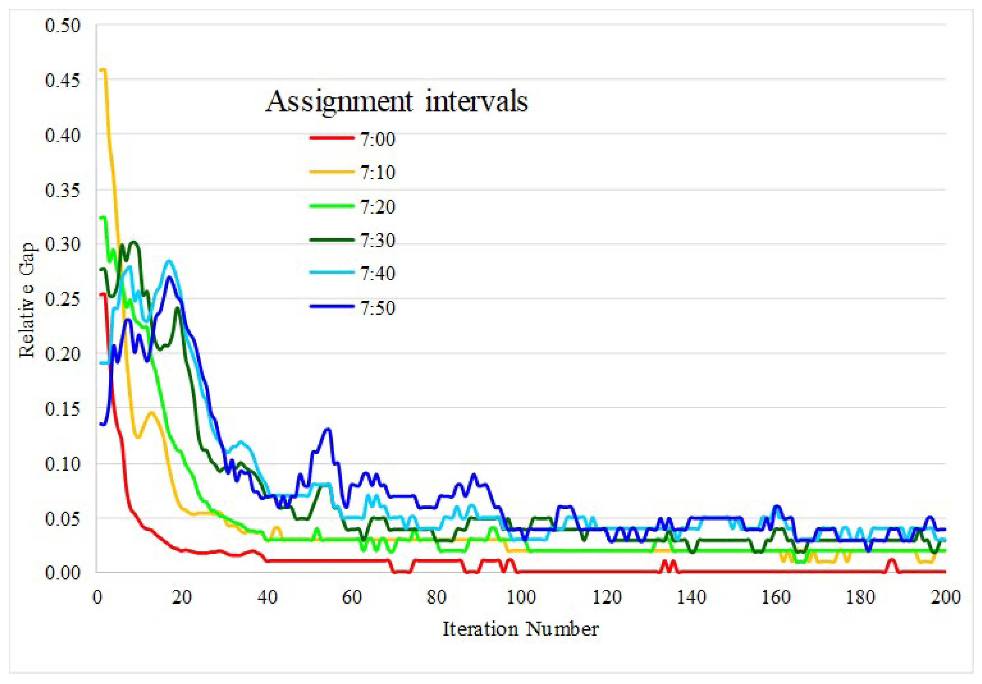
After running the DTA, it generated an output of model convergence to verify the path flow corresponding to each driver’s assumed behavior mechanism in trying to reduce their own travel time. Figure 11 shows that the convergence output, as the value of the relative gap in the initial assignment interval, increased with an increase in departure time as network congestion increased. Percentage variation in travel times increased for the used pathways, according to the same starting time period, then steadily decreased, while relative gap values increased to the 100th iteration. Beyond a set number of cycles, the designed assignment resolved effectively, with an overall average difference of 5%. After 200 iterations, the relative gap for any given departure time interval became constant.

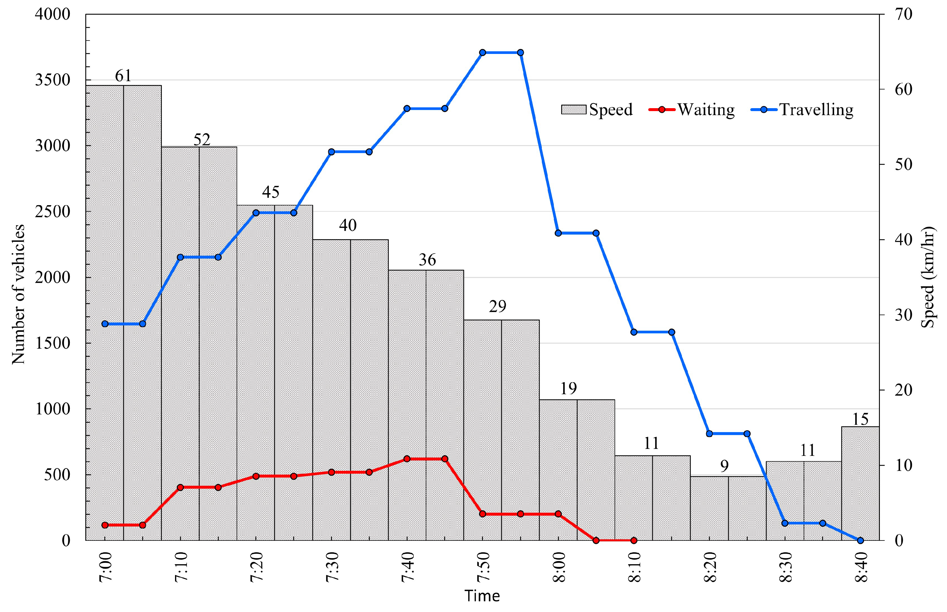
At every time interval, trip assignments were completed, indicating that almost all vehicles arrived at their destinations and exited the road network within the time period following the final demand loads. Figure 12 compares the total number of cars waiting to access the network (on virtual connections) at the conclusion of the interval, measured by the waiting time (red line). The total number of cars in the network at the conclusion of the period was assessed by traveling time. Demand of departures during the first time interval to the last demand loads used 11 time intervals (100 min) for network clearance. All vehicles arrived at their destinations and exited the road network within a time interval after the last demand loads.

The first time interval showed a non-congested situation and then traveling time increased and the network began to fill up. Congestion then occurred as well as cars waiting to enter the road network. Average speed continued to decrease, resulting in delay in the network until the sixth time interval. Then, no waiting caused the trend of traveling to decrease and speed increased.

5.2. Result of Scenario Evaluation

Urban floods affect transportation by increasing travel times, route changes, and congestion due to low speed. Roads with a flood depth of more than 50 cm are considered completely unusable by private vehicles. Therefore, evacuation timing demand in flood levels lower than 50 cm was assigned to evacuation centers and out areas to compare the efficiency of the road network under different flood conditions. Vehicles take the shortest path to reach their destinations but change to longer paths with longer travel time under flood conditions. For this model, variables of road function were degraded by flooding. Vehicles changed routes to reduce their travel time based on user equilibrium principles.

Table 2. Network performance indicators comparison.

	Performance Measure
Scenario	Speed (km/h)		VHT (veh-h)		VKT (veh-h)
	Value	Change (%)	Value	Change (%)	Value	Change (%)
Dry	29.72	-	3542.68	-	109,276.68	-
0–5 cm	27.70	−6.79	3794.14	7.10	109,220.79	−0.04
5–10 cm	21.29	−28.38	4835.76	34.08	109,634.47	0.33
10–15 cm	14.43	−51.45	7034.85	72.40	113,030.73	3.42
15–20 cm	8.57	−71.15	11,000.06	120.05	120,578.22	10.00
20–25 cm	4.08	−86.26	25,961.01	186.83	136,639.76	22.69
25–30 cm	2.03	−93.16	56,626,33	204.47	152,914.00	31.94

shows network performance indicators during the seven scenarios. Vehicle speed during the flooding scenarios changed. The average speed during dry conditions was 29.72 km/h. During the 0–5 cm flooding situation, speed decreased to 27.70 km/h, a 6.79% speed decrease. Similarly, 5–10, 10–15, 15–20, 20–25, and 25–30 cm flooding scenarios decreased vehicle speed to 21.29, 14.43, 8.57, 4.08, and 2.03 km/h, with percentage changes in speed of −28.38, −51.45, −71.15, −86.26, and −93.16 from the dry scenario.

Vehicle hours traveled (VHT) increased as vehicle speed decreased by 204.47% of travel time from the dry condition to the 25–30 cm flooding scenario. Vehicle kilometers traveled (VKT) also increased because, due to flooding, drivers choose alternate routes to reach their destinations. The VKT value in a flood of 0–5 cm was negative. Drivers may choose the fastest route by time but there may be a shorter distance because the overall performance of the whole network at the flood level was not different from the dry condition. Kilometers traveled increased by 31.94% compared to the dry condition for the 25–30 cm flooding condition. Results showed that flooding scenarios had a negative impact on network performance.

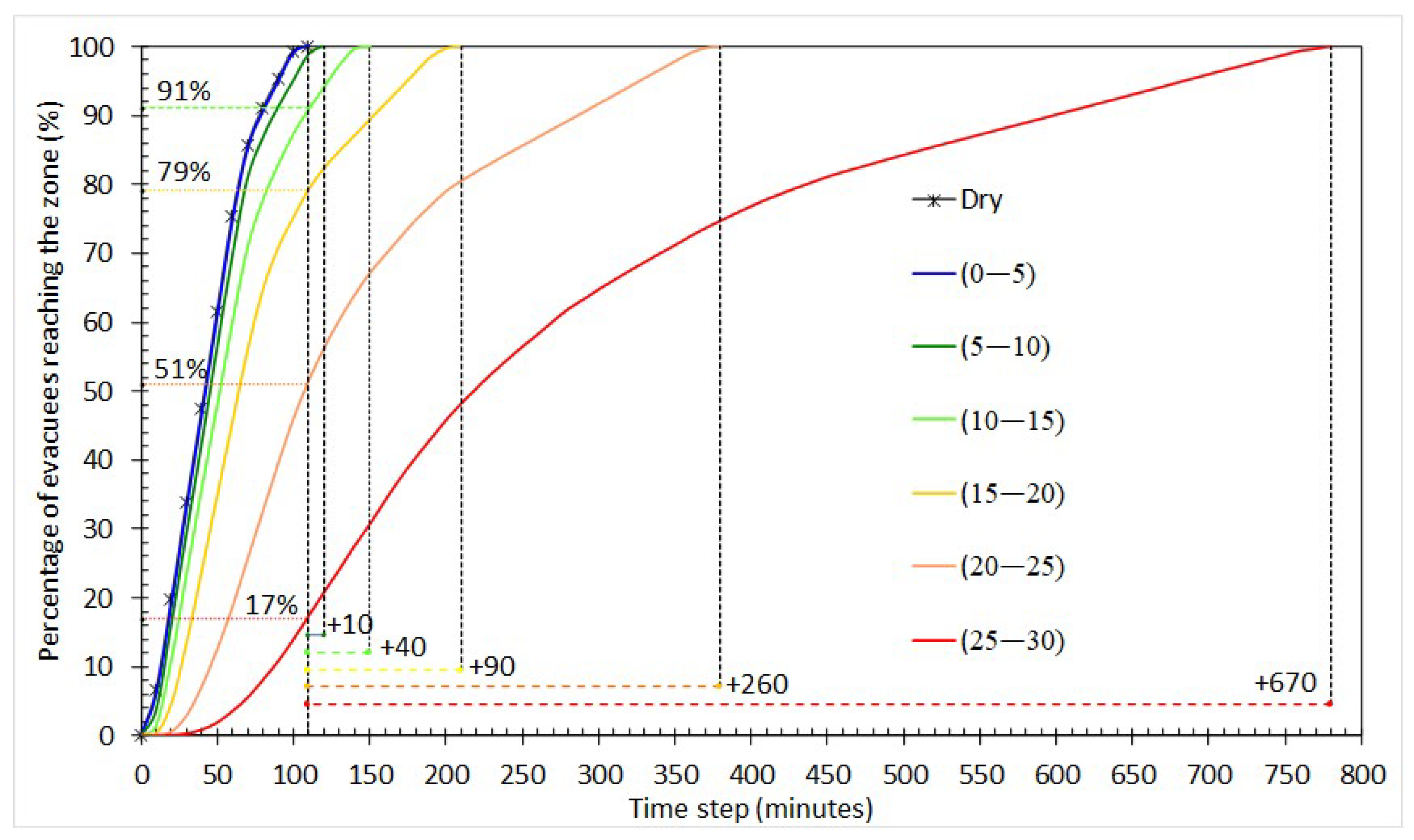
Figure 13 represents the seven scenarios plotted as a percentage of evacuation against time. Evacuation time for the baseline was “0” as dry. The evacuees took 110 min to arrive at evacuation centers, while none remained in the road network. The dry condition was compared to the seven scenarios. Evacuation time increased with deeper flood levels. For the 0–10 cm depth, evacuation time was not different to the dry condition. When flood levels increased to 10–15, 15–20, 20–25, and 25–30 cm, evacuation times increased to 40, 90, 260, and 670 min, respectively. The remaining evacuees increased with increasing flood levels. For flood levels of 10–15, 15–20, 20–25, and 25–30 cm, the percentages of evacuees remaining were 9%, 19%, 49%, and 83%, respectively.

6. Discussion and Conclusions

Hat Yai city, the economic and transportation hub of Songkhla province and southern Thailand, experiences heavy rainfall and flooding throughout the year due to northeast monsoon winds from October to January and southwest monsoon winds from May to October. Sudden flooding, in particular, makes it impossible for people to move and increases the risk of disaster. Therefore, people need to be evacuated quickly before flooding occurs to avoid injuries and deaths. Several scenarios were constructed by changing flooding situations and traffic volumes. Evacuation times in the study area were evaluated and compared for all scenarios with reference to dry conditions.

In this study, evacuation time was estimated and measures were identified for coming floods using past evaluation by providing dynamic alternate routes using DTA with a positive impact on network performance. Six flood level scenarios were used—0–5, 5–10, 5–10, 10–15, 15–20, and 25–30 cm—and compared with the dry situation. During flooding, the average speed dropped to 2 km/h, VHT rose above 200%, and VKT rose above 30%.

Cumulative evacuee arrival percentage showed that evacuees remaining in the road network increased when flood levels were higher than 5 cm. Flood levels of 10–15, 15–20, 20–25, and 25–30 cm represented percentages of remaining evacuees at 9%, 19%, 49%, and 83%, respectively. Time taken to evacuate increased according to flood level. For flood depths of 5–30 cm, travel time increased by 40, 90, 260, and 670 min, respectively. This suggests that it is necessary to start evacuation as soon as possible before the flood situation becomes serious.

This work was able to fully analyze the road network in depth to plan for route choice planning. The outcome of this study can be extended for actual operation, which can be identified to evaluate the road link that can be traveled the fastest in terms of travel time; the shortest available road network map will be provide this to the evacuation traffic planner. The avoidance route can be followed according to the historical data. The more necessary data to be included is the Flood Model for analyzing the road network flooding possibility. We conclude with some additional ideas to further expand on the topic of flood evacuation traffic management.

Integration of Emergency Response Plans: This study could explore the integration of emergency response plans into traffic management strategies during a flood evacuation. The study could analyze how different emergency response agencies can work together to coordinate traffic management efforts and ensure effective evacuation of affected areas. The study could also consider the role of public information campaigns in promoting awareness and preparedness among the public.

Evaluation of Evacuation Routes: This study could evaluate the effectiveness of different evacuation routes in reducing traffic congestion during a flood event. The study could analyze how different factors, such as road capacity, network connectivity, and population density, affect the efficiency of evacuation routes. The study could also consider the impact of natural features, such as rivers or mountains, on the availability of evacuation routes.

Assessment of Driver Behavior: This study could assess how driver behavior affects traffic flow during a flood evacuation. The study could analyze how different factors, such as age, gender, and experience, influence driver decision making during a flood event. The study could also consider the impact of driver emotions, such as fear and anxiety, on traffic flow and evacuation efficiency.

Use of Intelligent Transportation Systems: This study could explore the use of intelligent transportation systems (ITSs) to improve flood evacuation traffic management. The study could analyze how different ITS technologies, such as connected vehicles, traffic signal prioritization, and dynamic message signs, can be integrated into traffic management strategies. The study could also consider the impact of ITSs on reducing traffic congestion and improving evacuation efficiency during a flood event.

Consideration of Vulnerable Populations: This study could consider the needs of vulnerable populations, such as elderly people or people with disabilities, during a flood evacuation. The study could analyze how different factors, such as accessibility of evacuation routes and availability of transportation options, affect the ability of vulnerable populations to evacuate. The study could also consider the impact of community outreach and support programs on improving evacuation outcomes for vulnerable populations.