Staircase Wetlands for the Treatment of Greywater and the Effect of Greywater on Soil Microbes

Abstract

Fresh water is an increasingly scarce resource in both urban and rural development. As a response to this challenge, non-potable water reuse is on the rise. This research explored a potential off-grid system for water purification, consisting of a staircase wetland with terracotta pot plants working as a filter for greywater. This study further investigated the physicochemical properties of greywater and the soil before and after wetland purification. The removal of total suspended solids, total coliforms, fecal coliforms, etc., was always between 90 and 99%. Results show that the filtered water satisfied all requirements for water reuse, e.g., a pH of 7–7.5 and a turbidity < 5 NTU. This research then uniquely investigated the effect of greywater on soil microbes and soil biomass using soil DNA extraction and the tea bag index testing method. The filtered greywater absorbed by soil decomposed the soil faster (66% for green tea) and stabilized it better compared to tap-water-absorbed soil or unfiltered greywater. DNA generation sequencing revealed no significant differences in alpha diversity between the control and treatment samples. The beta diversity differences were significant. This nature-based solution can lead to reduced loads on the sewage system, resulting in less wastewater generation.

1. Introduction

The United Nations Sustainable Development Goal (SDG) Target 6.3 [1] states, “By 2030, improve water quality by reducing pollution, eliminating dumping and minimizing release of hazardous chemicals and materials, halving the proportion of untreated wastewater and substantially increasing recycling and safe reuse globally”. One action to achieve this goal can be in the form of nature-based solutions which are “actions to protect, sustainably manage, and restore natural or modified ecosystems, that address societal challenges effectively and adaptively, simultaneously providing human well-being and biodiversity benefits” [2]. Nature-based solutions promote nature as a medium for climate mitigation and adaptation, such as the use of untreated wastewater for sustainable practices. Untreated wastewater includes the so-called greywater (GW), which is defined as all household wastewater except for toilet flushes (e.g., wastewater produced in bathtubs, sinks, showers and laundry machines) [3]. With over two billion people living with high water stress globally [4], the reuse of generated GW from buildings is now imperative. A sustainable water usage technique can also reduce pressure on the sewerage systems of buildings. To use water sustainably, a nature-based solution in the form of a constructed wetland is a very eco-friendly strategy.

Constructed wetlands were the first nature-based solutions applied to GW treatment [5]. To improve water quality, constructed wetlands are a comprehensive approach to unify plant and microorganism security [6]. Constructed wetlands are man-made wetlands, designed and constructed like a natural wetland systems for the treatment of wastewater [7]. They also include a sand filter, usually as the last filtration layer of the GW treatment process. Compared to centralized systems, they have proved to be financially more advantageous in construction, operation and maintenance [8] This ascendency of the constructed wetland over conventional systems is due to its process stability under changing environmental conditions [9,10]. Currently, different types of wetlands are usually employed: surface flow wetlands, subsurface flow wetlands and hybrid systems [9]. Their differences lie in the flow of water. In surface flow wetlands, water flows above the ground, generally having a soil bottom, emergent vegetation and a water surface above the substrate, whereas subsurface flow wetlands are designed to keep the water level below the top of the rock or gravel media, thus minimizing human and ecological exposure [11]. Different types of constructed wetlands may be combined to utilize the advantages of the different systems [12] Vertical flow–horizontal flow (VF-HF) and horizontal flow–vertical flow (HF-VF) constructed wetlands are the most common hybrid systems [13]

In the last two decades, environmental, economic and energy benefits arising from the reuse of GW treated by nature-based solutions have been recognized, as follows:

• Environmental benefits include recovering water resources and minimizing sewage production [5].
• Economic benefits are reductions in water supply costs (through water recycling), which results in reduced household water bills [14].
• Energy benefits are in the form of limited energy generation per family per year from reused GW with installed turbines, pipe systems, storage and disinfection in high-rise buildings [15].

The use of domestic GW for irrigation is becoming increasingly common in both developed and developing countries to cope with water scarcity. In domestic households, GW is generated in high volumes with a lower level of pollution [16]. However, its use may affect microbial activity in the rhizosphere, which is the soil volume around the roots that is strongly affected by root functioning [17]. This classical definition describes the rhizosphere as a four-dimensional (4D) object: 3D for volume, and time for functioning [18]. The use or reuse of GW for growing plants may affect microbial activity, as the surfactants degrade the rhizosphere, along with the use of plant transpiration and subsequent condensation to purify water [19]. The effectiveness of microbial communities associated with the rhizosphere and the physiology and internal dynamics of plants play important roles in GW reuse. Moreover, GW has the potential to increase soil alkalinity if applied on garden beds over a long time. It was observed [20] that the reuse of GW with a pH above 8 can lead to increased soil pH and reduced availability of some micro-nutrients for plants, thus affecting their growth. Therefore it is essential to check the properties of soil and plants each year, at the same time of the year, to build up a track record [21].

Considering its benefits, the reuse of GW in buildings is a growing trend in the market [22,23]. This study aims to reduce water consumption in more households but can be scaled up for commercial buildings and industries in the future by reusing GW [24]. To investigate the effective use of GW, this research first reviews the literature about the available and existing nature-based solutions for GW treatment. Second, it identifies the properties, guidelines and policies on water reuse, defining an assessment matrix that can be employed to evaluate whether a GW treatment system is successful or not. Third, it undertakes an empirical investigation of a novel nature-based system, through the following: (a) water testing: physiochemical tests of the GW and tap water; (b) soil testing: physiochemical tests of soil; and (c) biomass findings: a tea bag index method and soil DNA extraction. Last, it draws conclusions and future recommendations for the efficient reuse of GW.

1.1. GW Classification, Parameters and Guidelines

GW can be classified based on the organic content, which is determined according to the source of the waste water, e.g., the GW collected from a kitchen sink has more organic content than GW from a bathtub. The two major types are light greywater (LGW) and dark greywater (DGW). LGW sources are bathrooms, showers, tubs, hand basins and bathroom sinks, whereas DGW includes laundry facilities (washing and rinsing), dishwashers and, in some studies, also kitchen sinks [9,25,26]. Further classes of these two types are based on the composition of GW related to the products/elements contained in that particular source, as shown in

Table 1. GW classes with ingredients; the standard classifications are Light (L) and Dark (D). Here, LGW and DGW are classified by A, B, and C, D.

GW Class	Origin	Products	Percentage of Total GW
Class A (LGW)	Washbasin	Hand washing soap, toothpaste, body care products, shaving waste and hair	50–60% [3]
Class B (LGW)	Bathroom	Body wash soap, shampoos, body care products, hair, body fats, lint and traces of urine
Class C (DGW)	Kitchen Sink	Food residues, high amounts of oil and fat and dishwashing detergents.	10% [27,28,29,30,31,32,33,34]
Class D (DGW)	Laundry and all other washing required spaces	Laundry soap, bleaches, oils, paints, solvents, non-biodegradable fibers from clothing and microplastics.	25–30% [35,36]

. In this research, nomenclature based on an alphabetical index is used to differentiate the GW origin.

The GW characteristics vary according to their origin [37]. The largest source of GW, with the least contamination, is Class A (LGW). Class A has only 7% of the total daily pollutant loads in domestic households [38] and originates from washbasins. Only parametric studies that have focused on washbasin or Class A GW are summarized in

Table 2. Physical, chemical and microbiological parameters of Class A GW (LGW) found in the literature and their range. Square brackets “[]” in the first column represent units. The third column represents the acceptable values by standards.

Physical Parameters [Units]	Values	Range
Turbidity [Nephelometric Turbidity unit, NTU]	164 [9], 84.3 [37], 35–164 [39]	Irrigation water quality standard < 10 [40] Fairly turbid (15–25) Rather turbid (25–35) Turbid (35–50) Very turbid > 50
Total solids (TS)	835 [9], 204 [41], 450.3 [37]	–
TSS [mg/L]	153–259 [9], 141.2 [37], 25–181 [39]	Irrigation water quality standard (≤33)
Total dissolved solids (TDS) [ppm]	473.3 [37]	Ideal drinking (0–40) Acceptable (40–100) Borderline (100–200) Average tap water (200–300) Possibly hazardous (300–400) Potentially hazardous (400–500+)
Chemical parameters
pH	7–7.3 [9], 7.43 [42], 7.96 [43], 7.2 [37], 6.72–9.82 [39], 6.7–9.8 [44]	Adequate for irrigation (6–8)
Biochemical oxygen demand (BOD) [mg/L]	155–205 [9], 109 [45], 155 [25], 100 [46], 568 [43], 138.5 [37], 33–305 [39], 35–92 [44]	Irrigation water quality standard (≤50)
Chemical oxygen demand (COD) [mg/L]	386–587 [9], 263 [45], 587 [25], 110 [46], 58 [41], 1171 [43], 340.5 [37], 47–587 [39], 47–350 [44]	Irrigation water quality standard (≤50)
Chlorides [mg/L]	237 [9]	Irrigation water quality standard (≤70)
Methylene blue active substances (MBAS) [mg/L]	3.3 [9]	–
Oil and grease (O&G) [mg/L]	135 [9]	–
Total organic carbon (TOC) [mg/L]	99 [25], 63 [46], 155.28 [47], 60.8 [37]
Total Nitrogen (TN)/NH3 [mg/L]	10.4 [9], 9.6 [45], 10.4 [25], 10.2 [46], 2.22 [47], 0.21 [41], 14.3 [43], 0.6 [37], 2.5–10.4 [39]	Irrigation water quality standard (≤5)
Total Phosphorous (TP) [mg/L]	2.58 [45], 0.13 [25], 0.15 [47], 2.25 [43], 1.1 [37], 0.3–2.6 [39]	Irrigation water quality standard (≤0.8)
N/TOC [mg/mg]	0.11 [25], 0.16 [46]	–
P/NOC [mg/mg]	0.001 [25]	–
Microbiological parameters
Total coliform (TC) (Most Probable Number, [MPN]	9.42 × 104 [9], 0.0–1.7 × 106 [44]	–
Fecal coliform (FC) [MPN]	3.50 × 104 [9]	–
Escherichia coli (E. coli) [MPN]	10 [9]	<1000 per 100 mL
Ground elements and heavy metals
Boron (B) [mg/L]	0.44 [9]	Irrigation water quality standard (≤0.75)
Calcium (Ca) [mg/L]	51.19 [47], 0 [41], 5.1 [37]	Irrigation water quality standard (≤120)
Magnesium (Mg) [mg/L]	7.25 [47], 0 [41], 1.8 [37]	Irrigation water quality standard (≤24)
Sodium (Na) [mg/L]	131 [9], 17.11 [41], 19.2 [37]	Irrigation water quality standard (≤30)
Sulfur (S) [mg/L]	27.70 [47], 2.12 [37]
Copper (Cu) [mg/L]	0.005 [47]	Irrigation water quality standard (≤0.02)
Zinc (Zn) [mg/L]	0.020 [47], 2.03 [37]	Irrigation water quality standard (≤2)
Potassium (K) [mg/L]	1.55 [47], 1.98 [41], 3.6 [37]	Irrigation water quality standard (≤20)
Iron (Fe) [mg/L]	2 [47], 0.17 [37]	Irrigation water quality standard (≤5)

.

The guidelines for GW reuse vary at the national, provincial and organizational levels worldwide, as shown in

Table 3. Guidelines on the parameters required for GW reuse according to different organizations/institutes.

Required Parameters for Reuse of GW	USEPA Standards [50]	UK/EU Water Standards [51,52]	NSW Government [49]	USEPA Reclaimed Water Standard for Water Closet Flushing [53]
Water quality
pH	6–9	6–9	5.5–7.5	6–9 (monitor 1/month)
TSS	<30 mg/L	<30 mg/L	30 mg/L
BOD	<30 mg/L	<30 mg/L	20 mg/L	<10 Monitor 1/week
Turbidity		0.1 NTU		<2 NTU continuous monitor
Pathogen criteria
TC	2.2 cfu/100 mL	2 cfu/100 mL	10 cfu/100 mL
FC	≤200 cfu/100 mL	≤200 cfu/100 mL		No FC/100 mL

. For example, the total concentration of coliforms is limited to 2.2 cfu/100 mL in the United States [48] but is reduced to 10 cfu/100 mL for the Australian state of New South Wales [49].

1.2. Soil Properties and Biodiversity

Understanding the GW reuse guidelines alone is not enough to ensure a safe and healthy ecosystem for plants to grow. It is also important to investigate the plant’s soil behavior due to GW. Water is a fundamental factor in determining the health of an ecosystem where plants can grow, especially regarding soil properties. By absorbing GW, the soil may be damaged by harmful microorganisms, impeding plants’ growth. In this context, soil microbial biomass (bacteria, fungi and protozoa), which is the mass of the soil organic matter’s living components, can be employed as a proxy for the overall health of an ecosystem. Microbial biomass decomposes plant and animal waste, as well as organic matter in the soil, releasing carbon dioxide. This process of putting organic matter back into soil stabilizes the soil with time.

Changes in microbial productivity can also be used to predict changes in overall soil organic matter [54]. The most common methods used to quantify the used soil microbial biomass are chloroform fumigation–incubation (CFI) and chloroform fumigation–extraction (CFE) [55], spectrophotometric methods [56,57,58], phospholipid fatty acids (PLFAs) from soil [59], the tea bag index (TBI) method, and the DNA sequencing method. In the mentioned methods, the TBI is the most economical method, and DNA sequencing provides the maximum information about microbes.

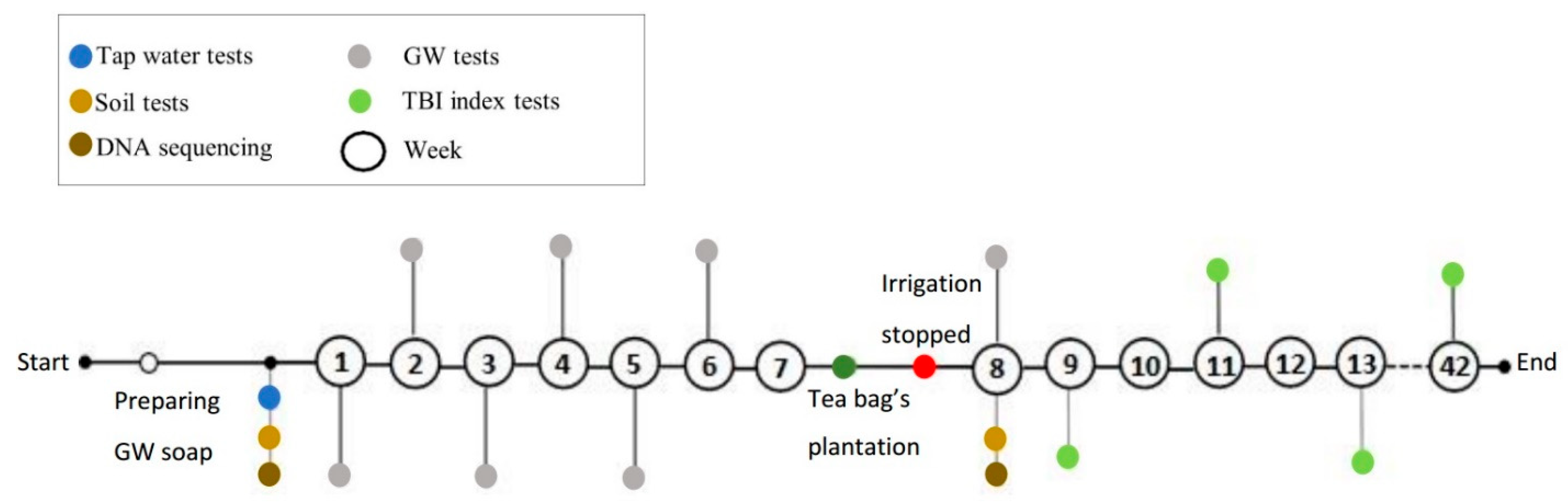
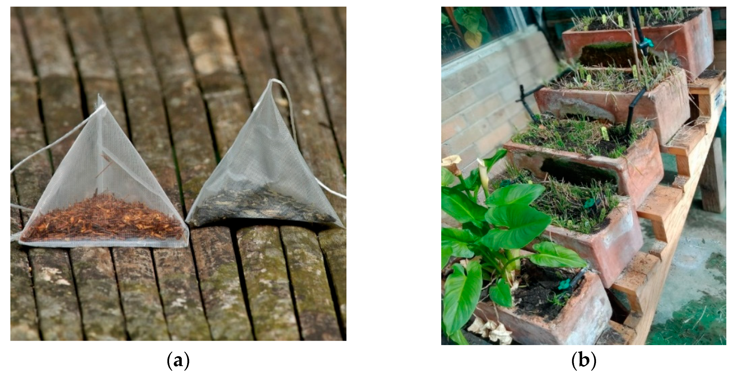
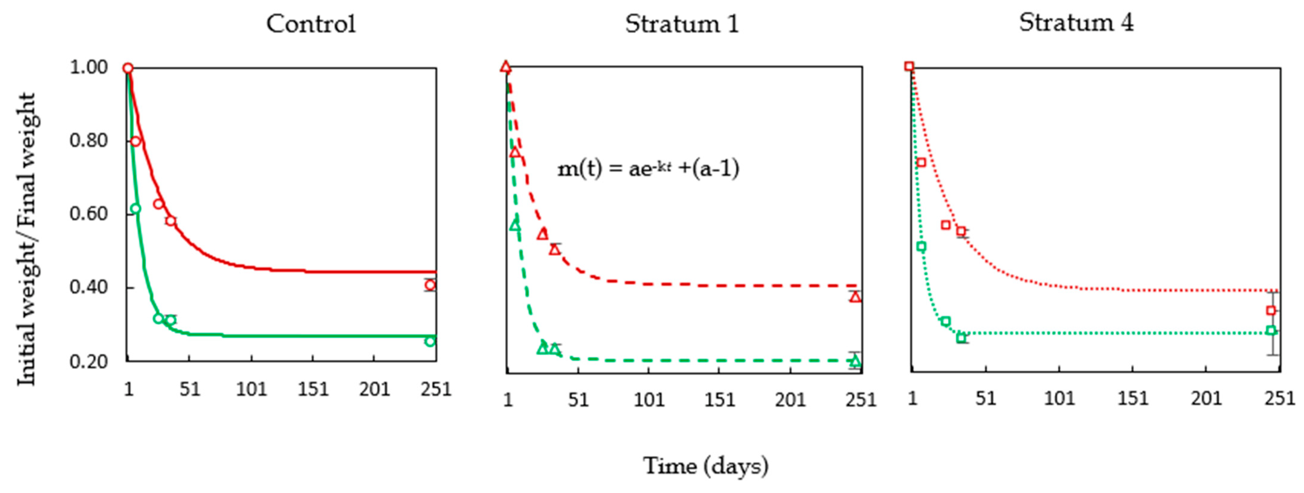
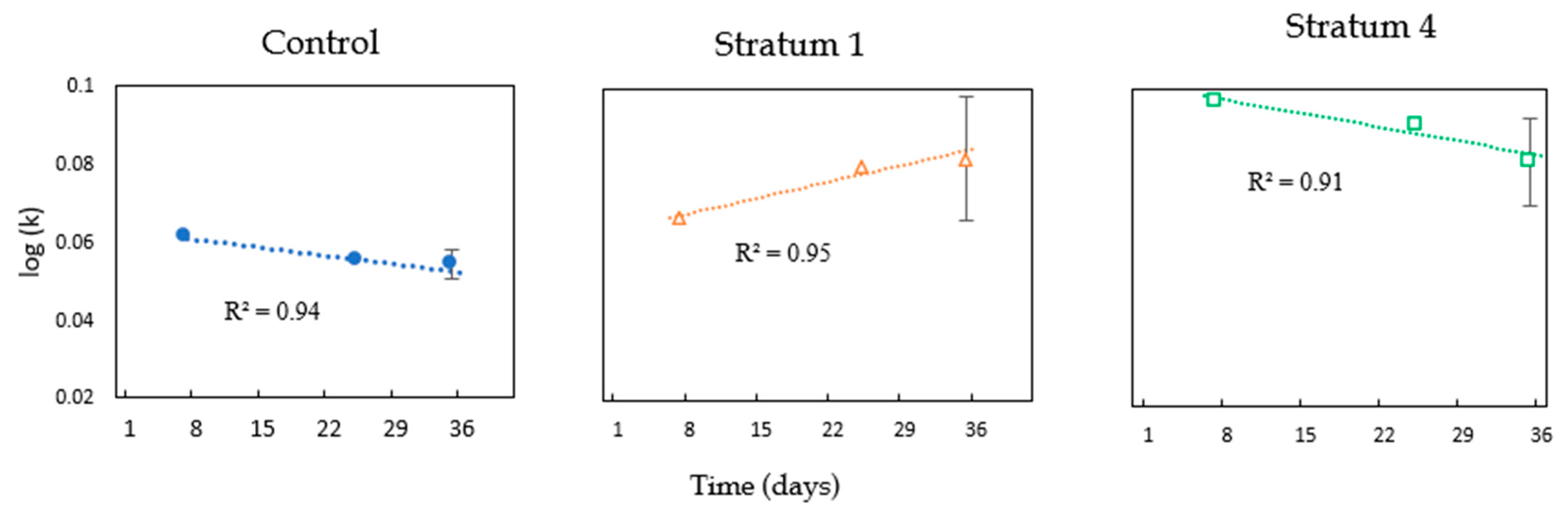
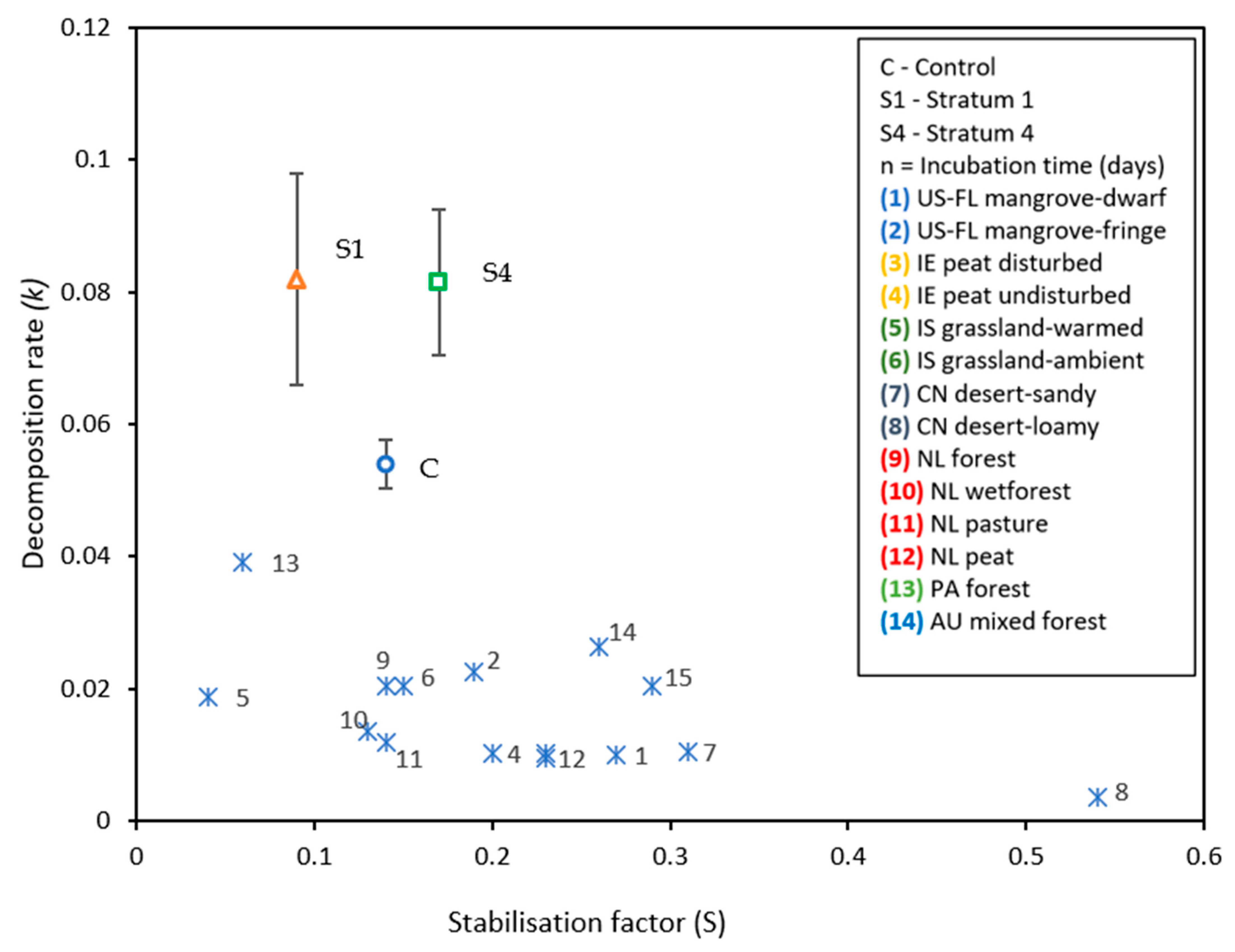
• The tea bag plantation method is used to find the decomposition rate of the soil that absorbs the GW. The tea bag index (TBI) method is a standardized and economical method used to quantify microbial-driven decomposition by measuring the tea mass after being buried in soil over a certain period [60]. This decomposition rate (k) results from increased microbial biomass (cell formations) and higher metabolic activity. Two different tea types are widely accepted for this test: rooibos and green. Each data point corresponds to a replica, i.e., a pair of tea bags includes one rooibos and one green tea bag. Rooibos tea is easy to decompose, whereas green tea is characterized by a slower rate of decomposition. The fraction of green tea that remains after the rooibos tea is fully decomposed is used to estimate the amount of biomass that is fixed in the soil, which is called stabilization (S). The TBI is calculated from both types of tea and is based on these two factors (S and k). Hence, the ‘S’ indicates the amount of material that remains in the soil, and ‘k’ is the amount lost as a byproduct of the decomposition. Both ‘S’ and ‘k’ are functions of the initial and final weights of their respective tea bags [60].
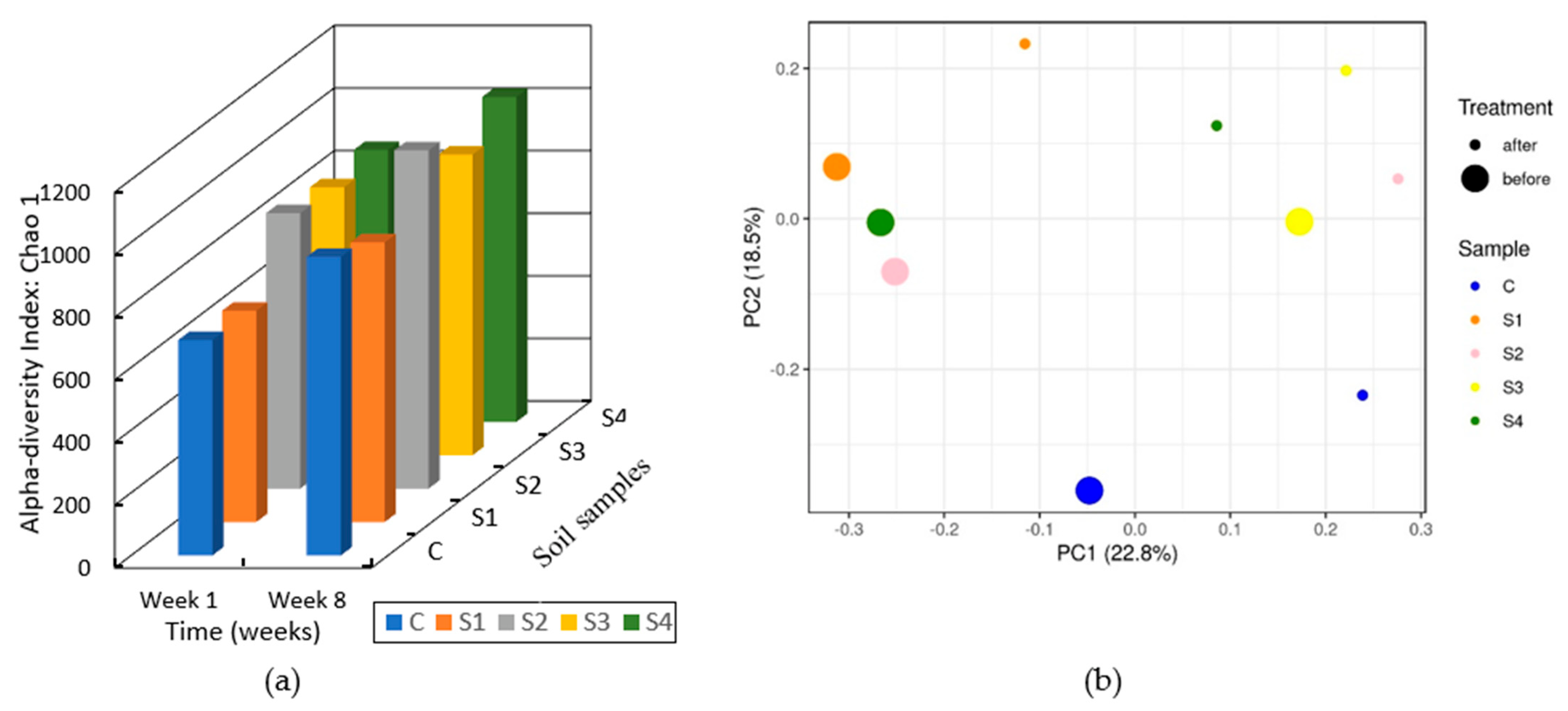
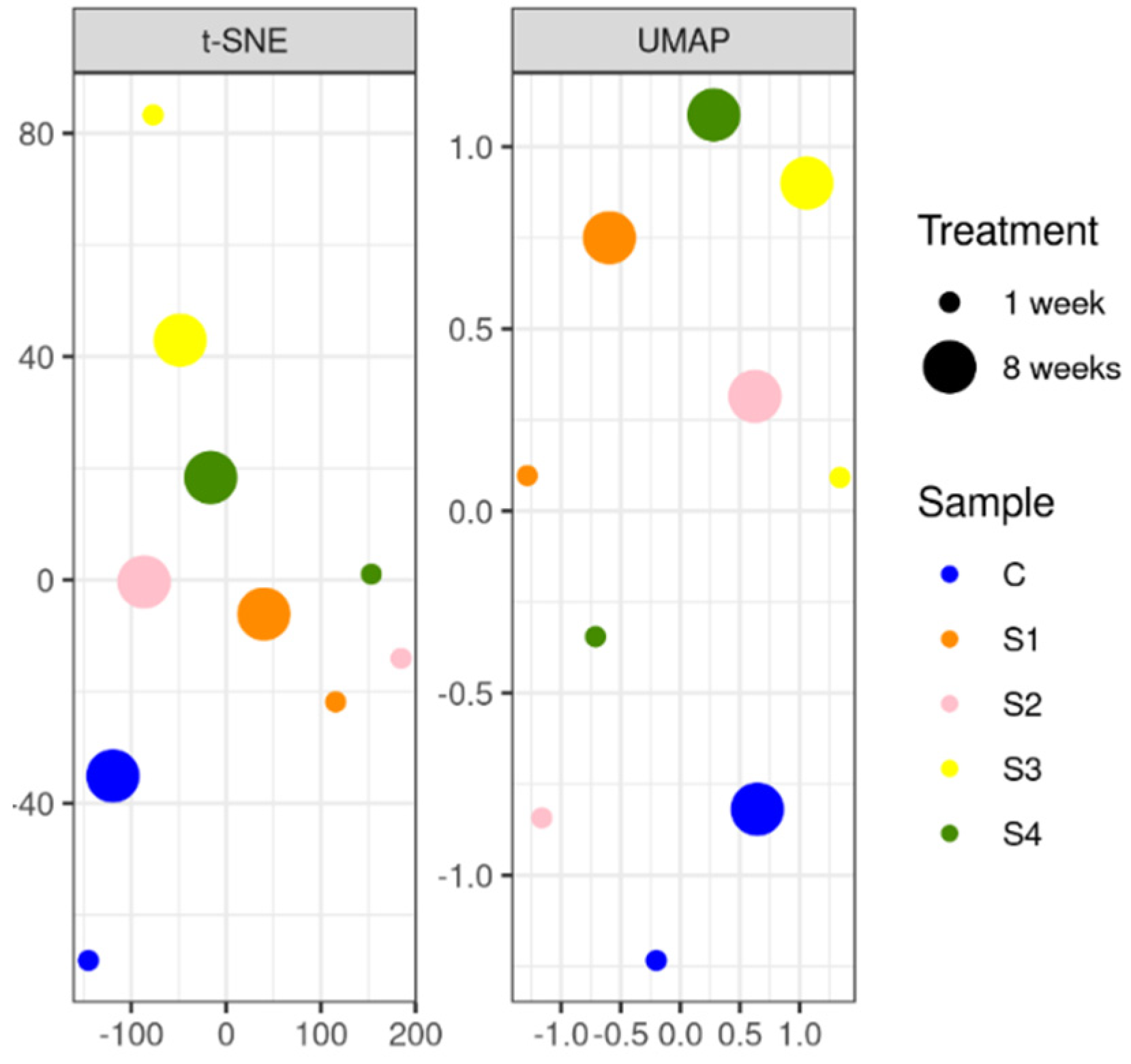
• DNA sequencing is a method used to gather information about organisms and their environment [61]. The sequencing is performed through a two-stage process. First, with commercial DNA kits, the cells are broken down, involving mechanical and chemical processes [62]. Second, short single-stranded DNA fragments, known as primers, are amplified by artificial replication [63]. The amplified DNA fragments are then sequenced, and a taxonomy of all the different kinds of bacteria is generated. Based on that taxonomy, diversity indexes are calculated, namely the alpha (α) and beta (β) [64]. α-diversity is local diversity, which counts the types of microbes in a sample [65]. As the species richness increases, the α-diversity of a particular sample also increases. β-diversity compares all the different kinds of microbes between two or more samples [66]. It gives an estimation of how similar or dissimilar the microbes of different communities are in different samples. Both α and β-diversity are determined from the phylogenetic tree, which is a representation of the evolutionary relationships among various taxa [67]. The α-diversity refers to the diversity within a particular habitat patch or ecosystem [68]. It corresponds to the number of species within a patch. Among patch diversity is the β-diversity, referring to the diversity between habitat patches or ecosystems. It corresponds to the total number of species that are unique to each of the ecosystems being compared.

The reuse of GW is an emerging field of research. However, despite the known effects of GW on soil physicochemical properties [69,70,71], the impact of GW on soil microbial species remains significantly underexplored. In this paper, for the first time, the impact of GW on the soil microbial species is studied. This research not only studies the quality of purified GW through a specific constructed wetland working as a filtering medium but also the effects of GW on the soil species using the tea bag index and DNA tests. This allows the microbial communities and multiple physicochemical attributes of the soil before and after absorbing GW to be correlated.

The first objective of the methodology is to filter GW coming out from the vanity (washbasin) of a washroom by passing it through a constructed staircase wetland, and second, to assess the impact of GW on the soil and protect the environment. Based on state-of-the-art review studies of GW treatments and reuse [72,73,74,75,76] or the impact of GW on the environment [5,77,78,79,80], the focus has been on treating or considering GW having same characteristics, e.g., the GW of washroom fixtures or kitchen fixtures are considered unit entities. Even if the characteristics of GW from a washbasin fixture (vanity) have been studied separately, as shown in Table 2, it has only been a brief overview of the mentioned parameters. As those parameters have only been compared with other fixture parameters but explicitly, its impact on the environment has not been studied. Moreover, in some studies [81,82,83], GW from laundry has been the focus because it has high level of surfactants, builders, bleaching agents and auxiliary agents or additives [81], which are difficult to filter compared to the GW of a washroom vanity.

Moreover, the exploitation of treated GW includes indoor reuse, such as flushing toilets, and outdoor reuse, such as irrigation and vehicle washing without considering the detailed in-depth impact of this water on environmental elements, e.g., the soil where it finally gets absorbed. This study not only streamlines GW reuse by focusing only on a single fixture (vanity) but also assess its impact on soil microbes. Studying the impact of a single fixture GW on soil up to the microflora level (bacteria, fungi, etc.) [84] is the knowledge gap that this study addresses.

2. Materials and Methods

This study employs the following testing protocol. First, GW soap was made that was similar in properties to Class A GW. Second, a novel prototype of staircase wetlands (vertical constructed wetlands) was designed and fabricated, and the capacity of the plants in the staircase wetland to filter and purify GW was tested for eight weeks. Third, a soil biomass study using the tea bag index and soil DNA sequencing tests was carried out (after GW treatment was stopped) to determine the effects of irrigating plants with GW. The sequence of the events and tests is shown in the methodology flow chart (Figure 1).

Physicochemical tests on the soil were performed after taking soil samples around the plant before and after the treatment of GW. Tea bag index testing was conducted after the GW supply was stopped. Similarly, the soil samples were also collected for a soil DNA study before and after passing through the wetlands.

The soil and water physicochemical properties before and after absorbing GW were evaluated according to the methods shown in Table 4. Except for pH and EC, all other tests were performed by Envirolab services in Sydney, NSW.

Table 4. Measuring methods/standards used for water and soil tests. Testing parameters 1.1, 1.2 and 2.2 were performed at The University of Sydney’s off-grid tech lab. Parameters 1.3, 1.4, 1.5, 1.6, 1.7 and 2.1 were performed by Enviro tech lab services in Chatswood. Parameter 2.3 was performed at The Metagen lab services in Queensland.

Testing Parameters	Measuring Method/Standards
1. Water tests
1.1 pH	Measured by Gro Line Waterproof Portable pH/EC (Hanna Instruments, Woonsocket, RI, USA)
1.2 Electrical conductivity	Measured by Gro Line Waterproof Portable pH/EC
1.3 Turbidity	Measured nephelometrically using Inorg-022 a turbidimeter, in accordance with APHA latest edition, 2130-B
1.4 TSS	Determined gravimetrically via filtration of the sample; samples were dried at 104 +/− 5 °C
1.5 BOD	Analyzed in accordance with Inorg-091 APHA latest edition 5210 D
1.6 TC	Australian standard 4276.5-2007
1.7 FC	Australian standard 4276.5-2007
2. Soil tests
2.1 Physiochemical tests
2.1.1 pH	Measured using a pH meter and electrode in accordance with APHA latest edition, 4500-H+.
2.1.2 Electrical conductivity (EC)	Measured using a conductivity cell at 25 °C in accordance with APHA latest edition 2510 and Rayment and Lyons.
2.1.3 Moisture content	Determined by heating at 105 °C (±5) for a minimum of 12 h
2.1.4 Total organic carbon (TOC)	A titrimetric method that measures the oxidizable organic content of soils
2.1.5 Total Nitrogen (TN)	Calculated as the sum of TKN (Total Kjeldahl Nitrogen) and oxidized nitrogen. Alternatively analyzed via combustion and chemiluminescence
2.1.6 Cation Exchange Capacity (CEC)—NH4Cl	Using 1 M ammonium chloride exchange and ICP-AES (inductively coupled plasma atomic emission spectroscopy) analytical finish
2.2 Biomass tests	Tea bag index (TBI) tests
2.3 DNA Extraction	Soil DNA sequencing

Table 4. Measuring methods/standards used for water and soil tests. Testing parameters 1.1, 1.2 and 2.2 were performed at The University of Sydney’s off-grid tech lab. Parameters 1.3, 1.4, 1.5, 1.6, 1.7 and 2.1 were performed by Enviro tech lab services in Chatswood. Parameter 2.3 was performed at The Metagen lab services in Queensland.

Testing Parameters	Measuring Method/Standards
1. Water tests
1.1 pH	Measured by Gro Line Waterproof Portable pH/EC (Hanna Instruments, Woonsocket, RI, USA)
1.2 Electrical conductivity	Measured by Gro Line Waterproof Portable pH/EC
1.3 Turbidity	Measured nephelometrically using Inorg-022 a turbidimeter, in accordance with APHA latest edition, 2130-B
1.4 TSS	Determined gravimetrically via filtration of the sample; samples were dried at 104 +/− 5 °C
1.5 BOD	Analyzed in accordance with Inorg-091 APHA latest edition 5210 D
1.6 TC	Australian standard 4276.5-2007
1.7 FC	Australian standard 4276.5-2007
2. Soil tests
2.1 Physiochemical tests
2.1.1 pH	Measured using a pH meter and electrode in accordance with APHA latest edition, 4500-H+.
2.1.2 Electrical conductivity (EC)	Measured using a conductivity cell at 25 °C in accordance with APHA latest edition 2510 and Rayment and Lyons.
2.1.3 Moisture content	Determined by heating at 105 °C (±5) for a minimum of 12 h
2.1.4 Total organic carbon (TOC)	A titrimetric method that measures the oxidizable organic content of soils
2.1.5 Total Nitrogen (TN)	Calculated as the sum of TKN (Total Kjeldahl Nitrogen) and oxidized nitrogen. Alternatively analyzed via combustion and chemiluminescence
2.1.6 Cation Exchange Capacity (CEC)—NH4Cl	Using 1 M ammonium chloride exchange and ICP-AES (inductively coupled plasma atomic emission spectroscopy) analytical finish
2.2 Biomass tests	Tea bag index (TBI) tests
2.3 DNA Extraction	Soil DNA sequencing

Figure 1. Flowchart of the GW methodology of the experiment. Black circles show the number of weeks from the start of the experiment. Events are shown on the horizontal line, and all the tests are shown through a vertical line with a colored dot head (legends).

Figure 1. Flowchart of the GW methodology of the experiment. Black circles show the number of weeks from the start of the experiment. Events are shown on the horizontal line, and all the tests are shown through a vertical line with a colored dot head (legends).

2.1. GW Soap Recipe

To produce Class A GW, water from the tap was mixed with a special GW soap, specifically designed for this experiment. First, products commonly found in washroom sinks were tested to assess their pH by mixing 10 g of each product with 50 g of water, as shown in

Table 5. pH and electrical conductivity (EC) of different products combined with water.

Products	pH	EC
Water + Shampoo	5.78	5.02
Water + Mouthwash	5.12	0.09
Water + Toothpaste	9.54	1.38
Water + Body wash	4.36	>6
Water + Laundry soap	10.72	>6

. The ingredients were tested with water to know their pH spectrum (acidic or alkaline). Products that could not blend well with the soap recipe, such as mouthwash, were not included.

The preparation of the GW soap followed a variation in the traditional soap recipe. First, 50 g of caustic soda was gently dissolved in 90 mL of distilled water to produce a lye solution. The solution was set to cool for 20 min. In the meantime, 200 g of coconut oil was melted in a microwave, mixed with 100 g of olive oil and, subsequently, mixed with the lye solution. The mixture was stirred in a stainless steel immersion blender for 10 min until the solution was emulsified. The solution was then heated slowly for 50 min and allowed to cool until it dropped below 80 °C. At this point, 40 g of toothpaste and 20 g of shaving cream were added to the solution. The mix was then added to a 650 mL plastic container and covered with a towel for a slow cooldown. After two weeks, soap-like synthetic GW was obtained, as shown in Figure 2a. Every week, a slice of the soap was placed in the wash basin sink, as shown in Figure 2b. The GW was supplied for a period of 8 weeks. In some weeks, to increase the effect of GW, the solution was made more concentrated.

To increase the number of coliform bacteria in the influent GW, a small quantity of sheep manure (15–20 g) was also added from the sink in specific weeks, mentioned in Section 3. This addition affected testing parameters 1.6 and 1.7, shown in Table 5.

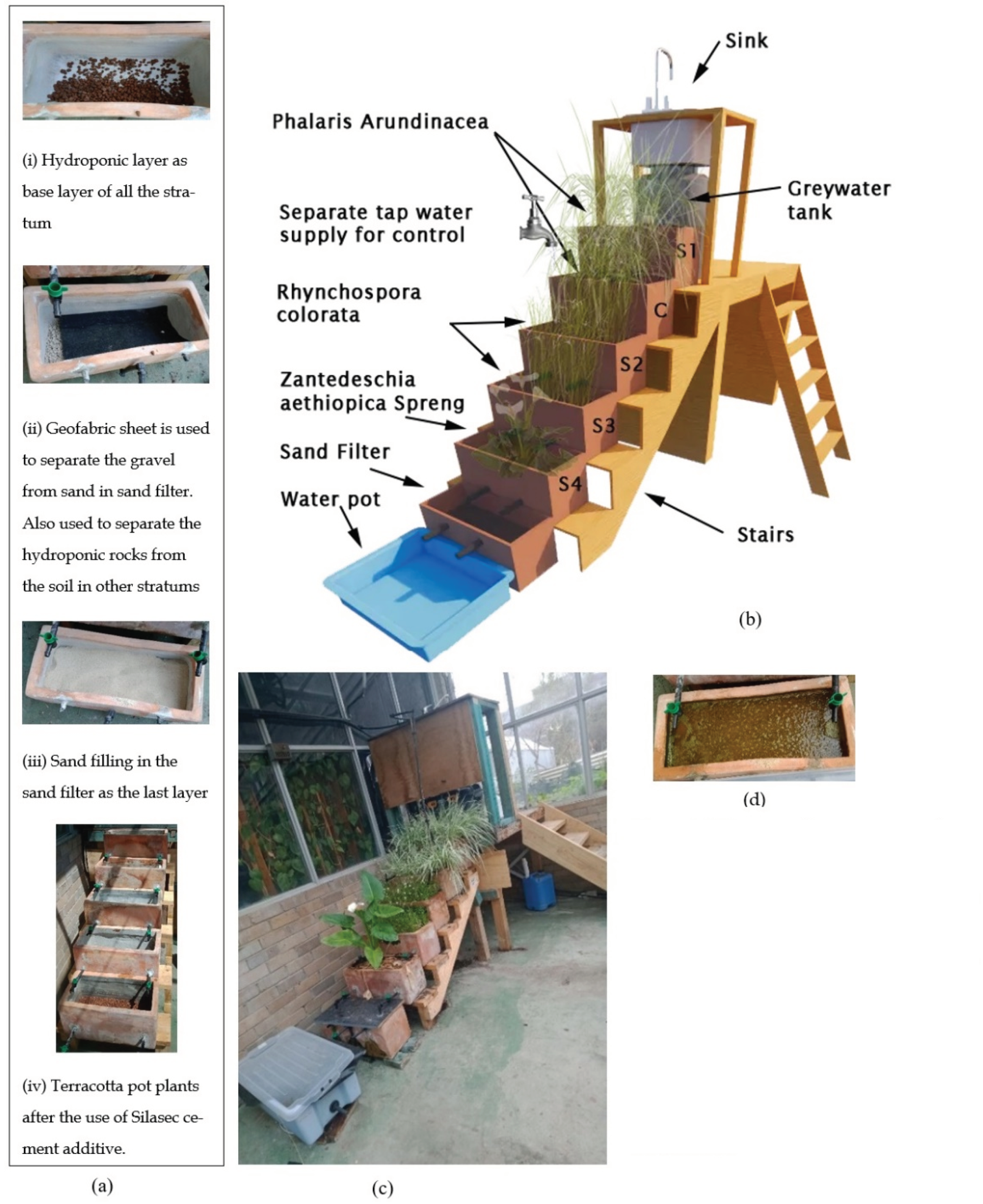
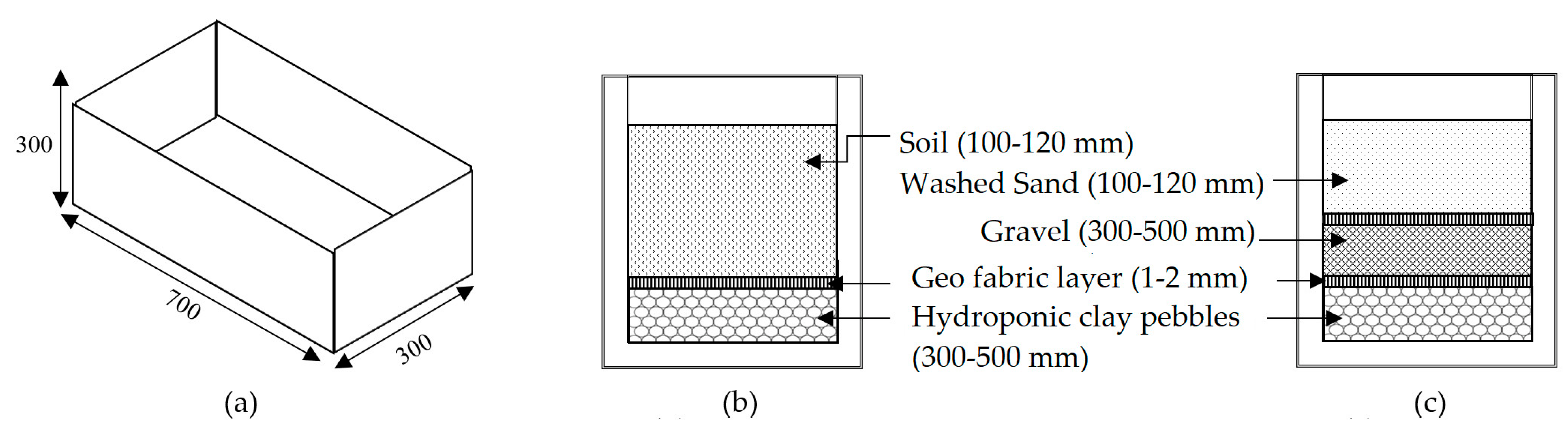
2.2. Construction and Arrangement of Staircase Wetland

A vertical wetland in the form of a staircase was constructed. The staircase provided a base for terracotta plant pots that contained the wetlands while allowing the GW to flow under the action of gravity through the wetlands. Weekly testing of the GW samples before and after passing through the staircase wetland was performed.

Five terracotta pots (70 cm × 30 cm × 30 cm) were placed on five steps of a staircase, giving the look of a staircase garden. The five plant pots contained five strata (S1, C, S2, S2 and S4), with each stratum at a different height from the ground. The second stratum was the control stratum (C), which was irrigated with tap water and did not receive any GW. Terracotta pots were used because they are made of durable natural material, with a traditional aesthetic sense. The heavy pots provided firmness when placed on the staircase. Moreover, the thick clay walls of the pots helped to buffer temperature changes, which can stress and damage the roots of plants [10]. A Silasec—a waterproofing cement additive [85]—was used on the inside of the plant pots, providing a protective barrier; the cement additive coating dried in 24 h, as shown in Figure 3a. Prior to placing substrate material layers within the system, holes were drilled on either side of the terracotta pots to allow for the flow of water from one pot to another under the action of gravity. Hydroponic clay pebbles were used as the first layer from the bottom. A sheet of geo fabric, shown in Figure 3b, was used to separate the soil from substrate media. The soil then slowly dispersed over each terracotta pot until it was a few centimeters from the top. Wetland plants were planted in each pot at a depth of 5 to 10 cm. Four of the strata (S1, S2, S2 and S4) were then connected utilizing a plastic pipe to allow for the flow of GW between each pot. The effluent flowed from one unit to the other under the action of gravity. Three plants were used in the constructed wetlands strata (S): Phalaris arundinacea (S1 and C), Rhynchospora colorata H. Pfeiff (S2 and S2) and Zantedeschia aethiopica Spreng (S4), as shown in Figure 2c. These plants are commonly known as Gardener’s-Garters, Starrush Whitetop and Calla Lily, respectively. All three were selected based on previous reports showing their efficiency in converting GW to potentially reusable non-potable water in the literature review and existing examples [86,87].

The soil in conjunction with the plant absorbs the nutrient-rich GW as it filters it into reusable GW. The different substrate media in the terracotta plant pots ensure that the contaminants from the GW are removed. Different small-diameter media (sand, clay pebbles and gravel) below the soil layer have shown effectiveness [88] in treating GW. These layers in the pots cause slow water filtration, giving enough time for microorganisms and plants to remove nutrients from GW and ensuring that no soil passes through from one pot plant to the next [89].

The sink at the top of the staircase was cylindrical, having a diameter of 36 cm and a height of 16 cm. The sink was programmed automatically to flow out 10 L of water a day (in equal intervals) to the GW tank placed below the sink, as shown in Figure 3b. The overflow of the GW from the tank was discharged into the terracotta plant pots. After filtering from the pots under the action of gravity, the GW progressed into the sand filter, and finally, the purified GW collected in a water tank, as shown in Figure 3b.

The system had a multi-layered sand filter, coated with silicon Silasec cement additive before arranging the substrate layers. Except for the washed sand as the topmost layer in the filter, there were layers of hydroponic clay pebbles (like the terracotta plant pots) and gravel at the bottom. The gravel layer was at the bottom to ensure adequate drainage The layers were separated by geo fabric. Plastic pipes from the fourth terracotta pot ran straight into the sand filter. Overflowed GW was collected in the water tank, and the retained GW in the sand filter created a biofilm layer, known as the Schmutzdecke.

Water samples were collected every week from the sink and the water tank. A cross-section of the pots and sand filter is shown in Figure 4b,c.

Figure 3. (a) Preparing the terracotta pot plants by arranging the substrate layers. (b) Three-dimensional model of the experiment, showing all the strata and their respective plant species (Phalaris arundinacea in S1 and C, Rhynchospora colorata H. Pfeiff in S2 and S4 and Zantedeschia aethiopica Spreng in S4). (c) Experimental set–up in the off–grid tech lab at The University of Sydney. (d) Developed biofilm layer (Schmutzdecke) in the sand filter.

Figure 3. (a) Preparing the terracotta pot plants by arranging the substrate layers. (b) Three-dimensional model of the experiment, showing all the strata and their respective plant species (Phalaris arundinacea in S1 and C, Rhynchospora colorata H. Pfeiff in S2 and S4 and Zantedeschia aethiopica Spreng in S4). (c) Experimental set–up in the off–grid tech lab at The University of Sydney. (d) Developed biofilm layer (Schmutzdecke) in the sand filter.

Physicochemical tests on the soil were performed after taking soil samples from the plant pots before and after the treatment of GW. Tea bag index testing was conducted after the GW supply was stopped. Similarly, the soil samples were also collected for a soil DNA study before and after passing through the wetlands.

The soil and water physicochemical properties before and after absorbing the GW were evaluated according to the methods shown in Table 5. Except for pH and EC, all other tests were performed by Envirolab services in Sydney, NSW.

2.3. Tea Bag Plantation in Staircase Wetland

The tea bag index (TBI) method uses code-specific Lipton™ brand bags (Westervoort, The Netherlands), i.e., pyramid bags—EAN 8,714,100,770,542 and EAN 8,722,700,188,438, shown in Figure 5a. They are distributed by specific European grocery shops, e.g., Dutch supermarkets and the Dutch Expat Shop. These particular Lipton tea bags from The Netherlands were used because they are standardized and tested tea bags used in the literature [60]. The tea bags were planted inside the soil in the form of replicates. Each replicate consisted of one green and one rooibos tea bag, making a pair. The primary reason for using two different types of tea bags in a single replicate was to assess the dynamics of two different types of materials under the same environment and conditions [60]. Coding was performed for the tea bag replicates based on their location, incubation time and replicate number, e.g., the S1t4R2 code given to a replicate meant Stratum 1, a time of 4 days, and replicate 2. The stratum (S) refers to the terracotta pot plant, the time frame (t) is the number of days (incubation time) that a replicate remained planted, and R2 means the replicate number (pair number) dug out at that particular t. The teabags were taken at incubation times (t) equal to 4, 7, 25, 35 and 246 days. The number of replicates varied for t = 4, 7, and 25 days, which had only one replicate, whereas t = 35 and 246 days had three replicates each (mean value was taken with error bars). The tea bags for t = 4 days were not considered because of getting damaged while digging them out.

The tea bags were planted on the day that the testing of the GW was completed. Before planting, the initial weight of the bags was noted, and a yellow tag was placed on the top of each replica’s plantation place to record the location, as shown in Figure 5b below.

Figure 5. (a) Tetrahedron-shaped synthetic tea bags used for tea bag index (TBI) experiments: rooibos tea (left) and green tea (right). (b) Yellow stacks placed on the top of tea bag replicates of the planted areas. The main events of the TBI experimental process are described below: Day 1: All replicates were weighed and planted in Strata 1, 2 and 5. Day 4: The t4 replicates were taken out and stored in the refrigerator at 4 °C. Day 7: The t7 replicates were taken out. To remove the wet soil and the moisture, the replicates were put in the oven for a week at 50 °C. Day 14: The replicates were taken out of the oven. The dry soil around the replicates was removed through desiccation, and their final weights were noted. Day 25: The t25 replicates were taken out of the soil and stored in the refrigerator. Day 35: The t35 replicates were taken out of the soil and placed in the oven alongside the t25 replicates for one week at 50 °C. Day 42: The t25 and t35 replicates were taken out of the oven. Day 246: The t246 replicates were taken out of the soil and then stored in the oven for 7 days before weighing their final weights. After desiccation, their final weights were noted.

Figure 5. (a) Tetrahedron-shaped synthetic tea bags used for tea bag index (TBI) experiments: rooibos tea (left) and green tea (right). (b) Yellow stacks placed on the top of tea bag replicates of the planted areas. The main events of the TBI experimental process are described below: Day 1: All replicates were weighed and planted in Strata 1, 2 and 5. Day 4: The t4 replicates were taken out and stored in the refrigerator at 4 °C. Day 7: The t7 replicates were taken out. To remove the wet soil and the moisture, the replicates were put in the oven for a week at 50 °C. Day 14: The replicates were taken out of the oven. The dry soil around the replicates was removed through desiccation, and their final weights were noted. Day 25: The t25 replicates were taken out of the soil and stored in the refrigerator. Day 35: The t35 replicates were taken out of the soil and placed in the oven alongside the t25 replicates for one week at 50 °C. Day 42: The t25 and t35 replicates were taken out of the oven. Day 246: The t246 replicates were taken out of the soil and then stored in the oven for 7 days before weighing their final weights. After desiccation, their final weights were noted.

The TBI method assumes that any litter incorporated into the soil consists of a labile (decomposable) and a recalcitrant (stable) fraction. Let M₀ be the initial mass of the litter and M_t be its mass at time t, to define the mass fraction as m(t) = M₀/M_t. The decomposition is assumed to obey an exponential law with two reaction rates [90]:

$$m=a{e}^{-kt}+\left(1-a\right)e^{-k^{\prime }t}$$

(1)

where a is the labile fraction, k is the decomposition rate of the labile fraction, (1 − a) is the recalcitrant fraction, and k′ is the decomposition rate of the recalcitrant fraction. The reaction rate of the recalcitrant fraction k′ is considered to be small in comparison to the labile fraction k, so that, for small times (k′t ≪ 1), Equation (1) can be reduced to

$$m\left(t\right)=a{e}^{-kt}+\left(1-a\right)$$

(2)

The TBI method uses two different litters: green tea, a labile litter, and rooibos, a more recalcitrant litter. They show contrasting decomposition rates. We use subindexes “g” and “r” to encode the parameters of the green tea and the rooibos tea.

The parameter of the exponential model of Equation (2) was obtained via non-linear regression. The range of values for variables ‘a’ and ‘k’ of Equation (2) was generated. Based on that range, the best possible fit was plotted. The generated curve touched most of the experimentally plotted points and the inferred values of a function where no experimental data were available.

If k is assumed constant, it can be obtained by isolating it from Equation (2):

$$k=\frac{1}{t}ln\left[\frac{a}{m\left(t\right)-\left(1-a\right)}\right]$$

(3)

In some cases, the reaction rate may change with time. This is the case of the fractal kinetics, which is characterized by a power-law dependency of the reaction rate with time [90]). In this case, the reaction rate can be calculated by considering two time points: t₁ and t₂ in Equation (1).

$$m\left(t_1\right)=a{e}^{-k{t}_1}+\left(1-a\right)$$

(4)

$$m\left(t_2\right)=a{e}^{-k{t}_2}+\left(1-a\right)$$

(5)

where m₁ and m₂ are the fractions (m₁ > m₂) of the rooibos biomass that remains after incubation times t₁ and t₂ (t₂ > t₁). The reaction rate ‘k’ can be computed by isolating k and a from Equations (6) and (7). The resulting equations are:

$$k=\frac{1}{t_2-t_1}\ln \left[\frac{m_1-\left(1-a\right)}{m_2-\left(1-a\right)}\right]$$

(6)

$$a=\frac{m_1-m_2}{e^{k{t}_1}-e^{k{t}_2}}$$

(7)

These equations can be solved iteratively by using an initial guess for ‘a’ chosen from the range given by the curve fit in Equation (2); then, k is computed from Equation (6). Next, a is corrected using Equation (7). The parameters k and a are iteratively calculated using Equations (6) and (7). By using an appropriate initial guess value of ‘a’, this procedure is applied until k converges to a given value.

During this decomposition, some parts of the labile compounds stabilize and become recalcitrant tea [91]. Environmental factors play an important role in this stabilisation [92], resulting in a deviation in the actual decomposed fraction (i.e., limit value) ‘a’ from the hydrolyzable (i.e., chemically labile) fraction H. This aberration can be interpreted as the suppressing effect of the environmental conditions on the decomposition of the labile fraction and is referred to as the stabilisation factor S.

The stabilization factor (S) is calculated as follows [60]

$$S=1-\frac{a_g}{H_g}$$

(8)

where H_g is the hydrolyzable fraction of the green tea equal to 0.842. This constant value of H_g for green tea is quantified via the method proposed by Van Soest [93], in which the use of two detergents divides the plants cells into less digestible cell walls and mostly digestible cell contents (contains starch and sugars).

The decomposable fraction of rooibos tea a_r is predicted as follows:

$$a_r=H_r\left(1-S\right)$$

(9)

where H_r is the hydrolyzable fraction constant of rooibos tea.

2.4. Soil DNA Tests

Before the treatment of GW, the soil samples (300 g) from each stratum were taken and stored at a temperature of −18 °C. After the treatment of GW was completed, another 300 g sample from each stratum was taken. All the soil samples were sent to the Metagen lab in Queensland [94] for DNA sequencing.

2.5. Statistical Analysis

Statistical analyses were performed in the Microbiome Analyst [95] and R environment [96]. The high-dimensional β-diversity data generated in the Microbiome analyst tool were further studied in the R environment using the UMAP and t-SNE analysis data techniques. UMAP (Uniform Manifold Approximation and Projection) [97] and t-SNE (t-distributed stochastic neighbor embedding) [98] are novel manifold learning techniques used for dimension reductions. Both take high-dimensional data and output a low-dimensional graph, meaning that a graph can easily be looked at by showing the same relationship seen in high-dimensional data.

In this study, the first distinction (α and β diversity) was the focus. The Chao 1 technique for the qualitative α-diversity and the Bray–Curtis dissimilarity index for the qualitative β-diversity were used. Moreover, the taxonomic phylum classification was studied.

3. Results and Analysis

The experimental results are organized into three sections: water tests, soil tests and soil biomass (tea bag index and DNA sequencing).

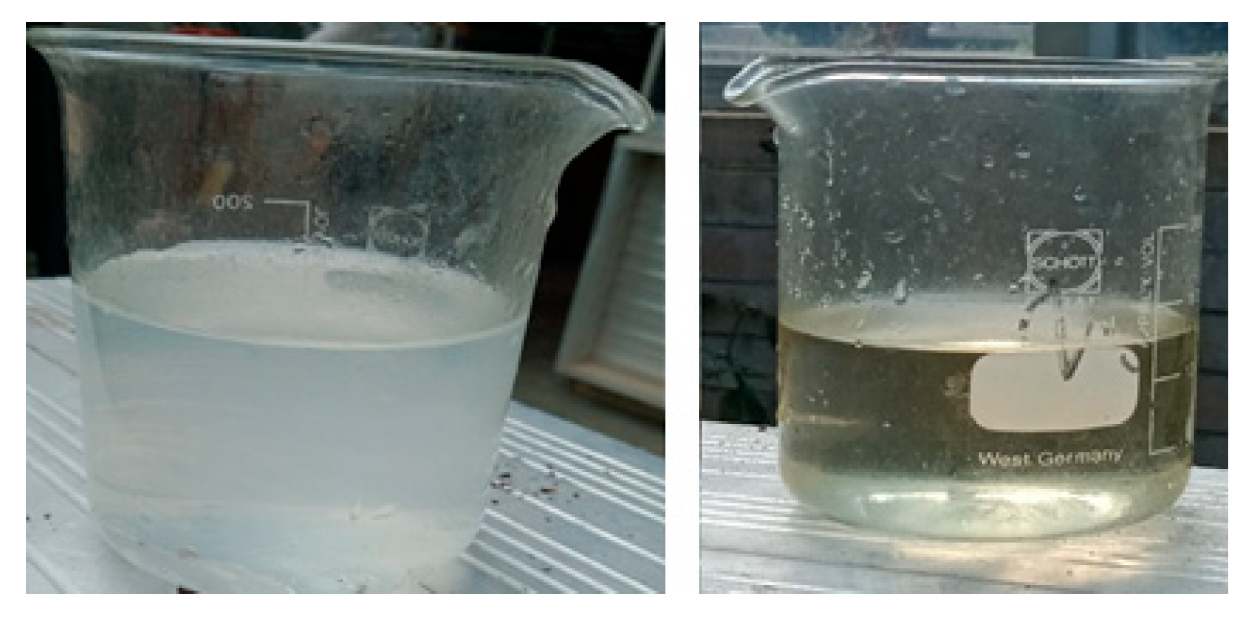
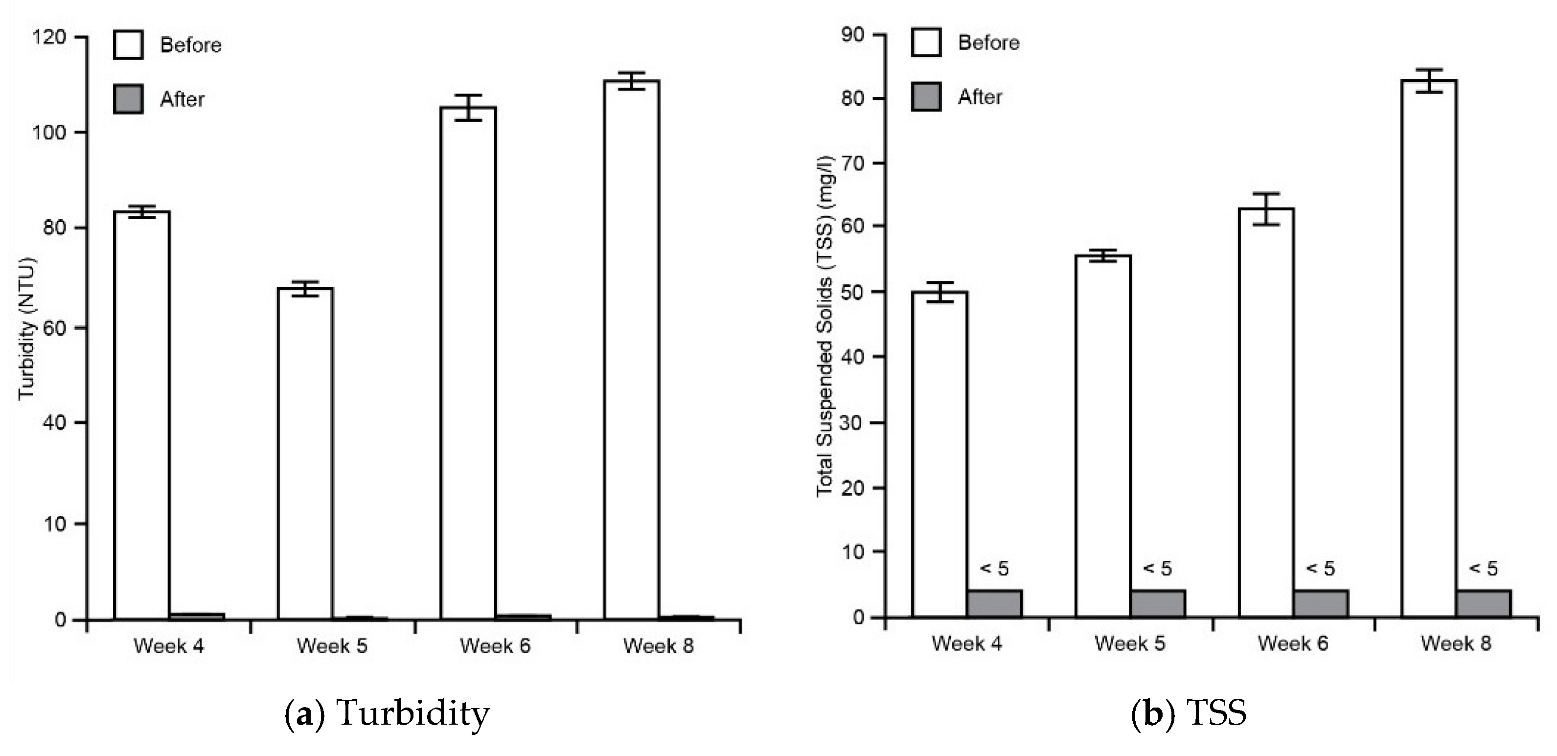
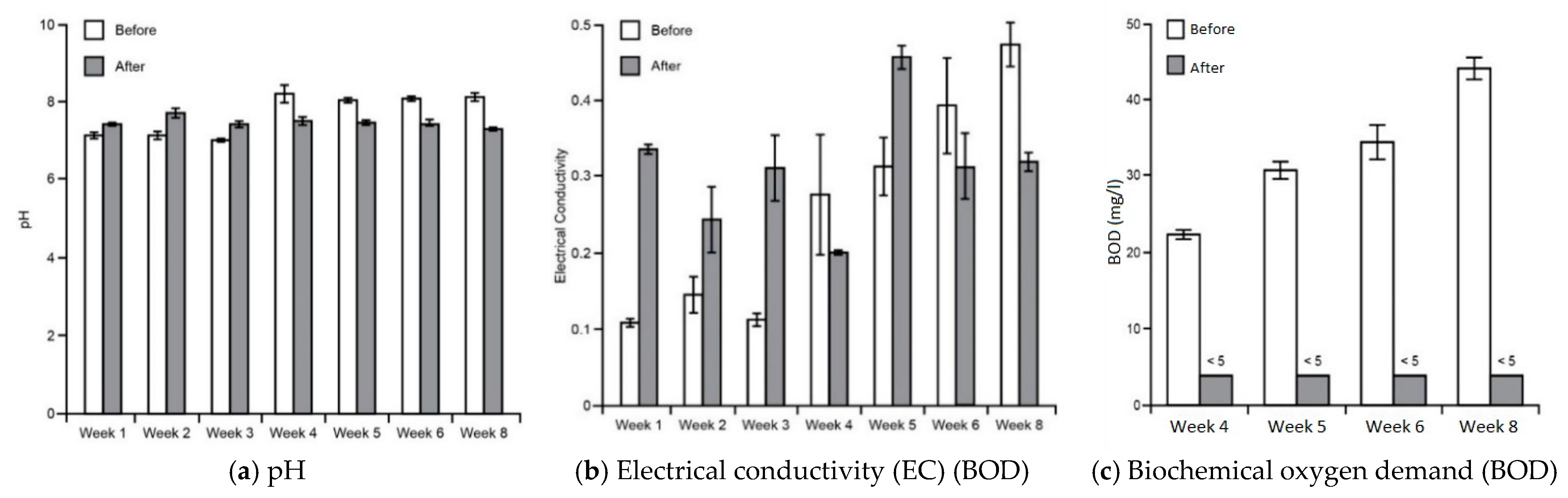
3.1. Water Tests

First, the tap water parameters were tested. The tap water only irrigated the control sample (C). The properties of tap water were found to be a pH of 6.8, an EC of 0.23 mS/cm, a turbidity < 5 NTU, a TSS < 5 mg/L, an FC < 10 cfu/100 mL, a TC of 92 cfu/100 mL and a BOD < 5 cfu/100 mL. These properties were in the range of the local required water quality standards [99,100].

The GW results contain ‘Before (influent)’ and ‘After (effluent)’ samples of water, shown in Figure 6a,b respectively. The Before samples were the samples of water that were collected before the treatment of GW, and the After samples were collected after the soil was treated with GW.

The turbidity levels were very high in the Before samples, shown in Figure 7a, but the After samples always fell in the range of acceptable standards for irrigation water, as <5 NTU for turbidity was noted in all the After samples. The sand filter was the primary factor in this decrease in turbidity [101], because a treatment technology using constructed wetland in a VF reduced effluent levels of GW to 8.1 and 16.9 NTU only [102], whereas in another HSSF study [103], in a temperate climate, the acceptable level of turbidity according to the US EPA was not met even once for a year-round analysis. The filtration system of the staircase wetland always kept the TSS value of the After samples shown in Figure 7b within the acceptable range of water quality standards. This filtration system performed better compared to another VF and HF wetland plant filtering medium study [102], in which the TSS was reduced to 10 and 34, respectively, for treating GW. This is also an indication that VF set-up in a constructed wetland performs efficiently compared to an HF set-up, whereas in a temperate climate study [103], the TSS was reduced below 5 mg/L only in the winter season.

In Figure 8a, for the first three weeks (Week 1–3), there was no significant change noted in the pH of the Before and After samples because the GW entering and leaving the system had an approximately equal pH range of >7 or <7.5. To check the credibility of the system, it was important to make the GW solution more concentrated while entering the wetlands. Therefore, the pH of the water entering the system (Before samples) was made more alkaline and was >8 from weeks 4 to 8, but the water leaving the system (After samples) ranged again from >7 to <7.5. The purified GW remained in the acceptable standards shown in Table 3. The EC value for the Before samples kept increasing over time, as shown in Figure 8b. The After samples started at 0.34 mS in the first week and increased to 0.48 mS by week 8. An increase of 0.1–0.15 mS per week was noticed from week 3 onward because the concentration of GW increased during that week. This meant that increased concentrations of GW resulted in an increase in EC, also shown in [104]. The purified GW EC value always remained in the acceptable level for irrigation water (<1.5 mS/cm) [105].

The BOD value for the water entering the system (Before samples) increased with time at an average rate of 7.22 mg/L per week, as shown in Figure 8c. This rate of increase was related to the accumulation of GW in the GW tank over a period of time [106]. The BODs of the After samples were always found below 5 mg/L, satisfying the water reuse guidelines mentioned in Table 3. A similar significant reduction was noticed in BOD removal when a reedbed plant (wetland plant) was used for GW treatment for the purpose of a low-cost solution [107]. The maximum retention time used in the low-cost media study was also 7 days (similar to this study). A BOD range from 1 to 10 mg/L in the After samples (effluents) is commonly reported [108].

Despite increasing the fecal and TC values by ten times (from <10 to <100) for the Before samples starting from week 5, shown in Figure 9a,b, the filtration system of the staircase wetland still produced acceptable water quality values for the After samples. This meant that the system was capable of cleaning even higher volumes of fecal matter and TC. The fecal and TC values were always reduced by 90% and 99%. This system performed better compared to another 10 L/day water consumption study [107] in dry and wet seasons, in which fecal caliform levels were not brought to the required reuse standards, using crushed rocks as a filtering medium with plants.

The GW sampling results proved the credibility of staircase wetland filtering because all parameters after GW treatment were in the range of local and international standards (mentioned in Table 3) or in the same range as that of tap water. The water retention time of the purified GW in the water pot was 7 days. From weeks 6 to 8, the retention time increased to 14 days, but the results were still the same for all parameters. The only visible difference with the After samples was a light brownish color, which was because of the soil type used in the terracotta pot plants. The used soil was highly organic, causing increased dissolved organic carbon, making the After samples light brown [109].

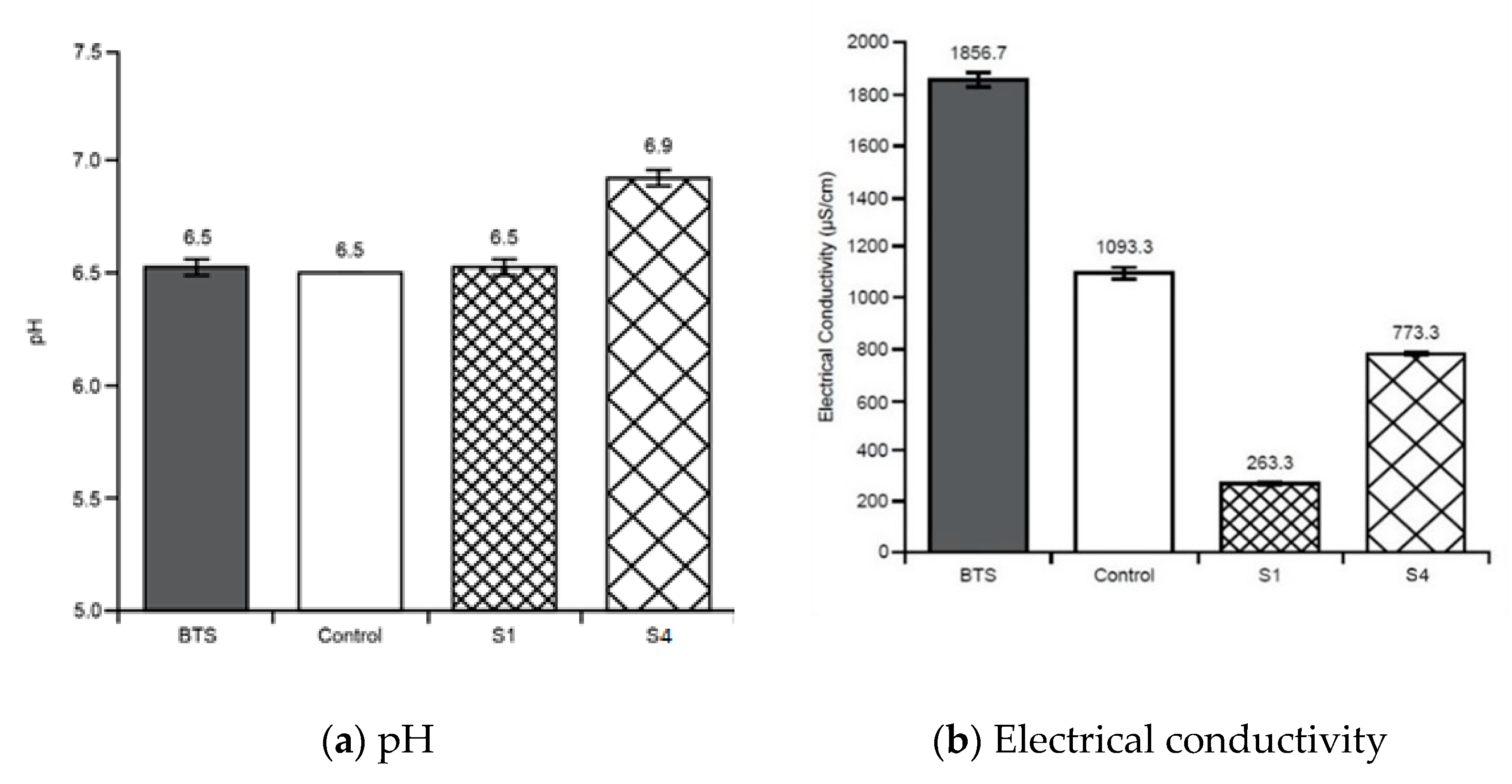
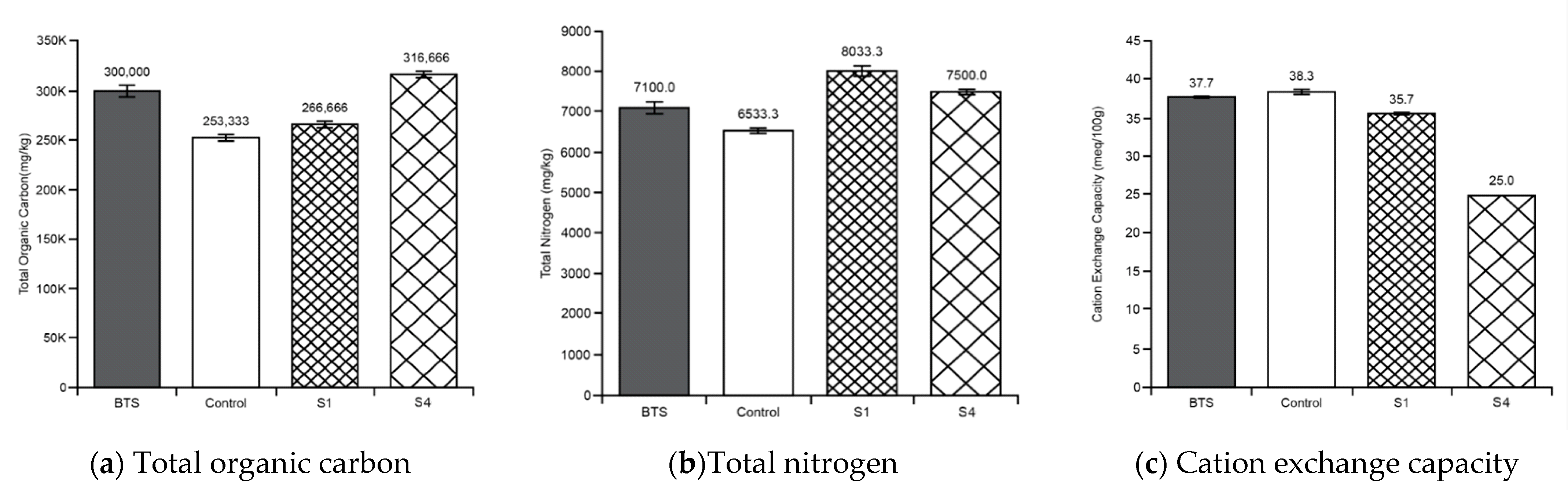
3.2. Soil Tests

Physiochemical tests of soil were performed to measure different soil parameters, i.e., pH, electrical conductivity, total organic carbon, total nitrogen, and cation exchange capacity.

The soil pH values in Figure 10a for all the strata showed no significant change compared to the Before treatment; a normal soil pH varies between 6.5 and 7.2 [110]. Acidic soils have a pH of <7, and basic soils have a pH of >7 [111]. The soil became neutral, shown by Stratum 5 having a pH value of 6.9 at the end of the experiment, due to the action of hydroponic rocks as the base layer in all the strata, but overall, the GW was not found to disturb the soil pH. Electrical conductivity is a soil property that is associated with the nature of the soil’s composition (particle size distribution, mineralogy), structure (porosity, pore size distribution, connectivity), water content and temperature [112]. It measures the amount of salt in the soil (salinity of soil). The EC before testing the soil sample (1856 µS/cm) shown in Figure 10b was in the range of fair to poor, according to the EC suitability irrigation chart [113]. With the GW treatment, it became 773 µS/cm in Stratum 4, which falls in the range of good to fair, also making it non-saline [114]. The EC in Stratum 1 was 263 µS/cm because of the high quantity of GW. The use of GW treatment left a positive impact on the EC of the soil.

Soils that have a total organic carbon (TOC) percentage > 18% are considered highly organic. As shown in Figure 11a, the control and Stratum 1 soil samples had approximately the same TOC percentage of 25% and 26%, respectively (1 mg/kg = 0.0001%). The GW treatment and filtering across all the strata resulted in an increase of approximately 7% in S4. There was a decrease of 5% in the control soil sample, which means that the TOC was directly proportional to the use of GW treatment. TOC transcends all chemical, physical and biological soil property categories, thus being recognized as the most significant single soil health indicator [115,116], and it is tied to several soil functions [117]. The percentage of total nitrogen (TN) was found to be low in the used soil, as shown in Figure 11b. The Before testing soil sample only had 7100 mg/kg (0.71%) of TN. Soil TN plays a key role in pedogenic processes, in addition to contributing to soil fertility [118]. The maximum TN that was found was in Stratum 1, which was only 1% more than the Before testing soil. The GW treatment did not increase the TN levels in the soil. Cation exchange capacity (CEC) is the total capacity of soil to hold exchangeable cations. Soil with a CEC > 20 meq/100 g is considered to have characteristics of heavy clay soils and organic peats [119]. Moreover, such soil has a high nutrient status and a high-water-holding capacity. In this study, all the strata had values > 20 meq/100 g, as shown in Figure 11c. Due to filtration in the staircase wetlands, the CEC value kept decreasing from Stratum 1 to Stratum 4 and decreased by approximately 34% in eight weeks.

3.3. Soil Biomass

3.3.1. Tea Bag Results

This project enabled 30 tea bag index in-field incubations (replicates included). However, not all the tea bag incubations ended in completed or meaningful measurements. The reasons for this incompletion include tea bags getting damaged during the withdrawal process from the soil or remaining inside the soil for too long (296 days), resulting in complete decomposition. The ratio of the final weight to the initial weight of green and rooibos tea bags (in the control and Strata 1 and 4) is shown in Figure 12.

The green tea mass loss averaged 62% in C and 66% and 63% in S1 and S4, respectively. The rooibos tea mass loss averaged 39%, 39% and 43% in C, S1 and S4, respectively, as shown in Figure 12.

The decomposition rate patterns for all the strata are shown in Figure 13 and Figure 14. The mean decomposition rates for incubation time (t) 0 to 35 were 0.05 ± 0.0015 in C, 0.08 ± 0.0033 in S1, and 0.08 ± 0.0030 in S4, as shown in Figure 13. The decomposition rate decreased non-linearly in C and S4 but increased in S1. A gradual increase of approximately 3% was noted in the S1 decomposition rate, from 25 to 35 days of incubation, indicating the gradual opening of the tissue’s internal structure by the microflora [81]. The main reason for this increased decomposition with time in S1 was the decrease in the concentration of the GW because the irrigation was stopped. The carbon:nitrogen (C:N) ratio increased in S1 from 33:1 to 42:1 in S4. The soil samples were taken before the TBI experiment started; therefore, through the filtration of the wetlands, the carbon accumulated in S4. If more soil tests had been conducted later (during the TBI experimentation phase), the C:N ratio would have decreased.

A high decomposition rate (k) was found in S4 initially, and the main reason is the high TOC and pH values in S4 (shown in Figure 13) compared to those of S1 and C. The degradation processes increased the pH to between 6.5 and 8 [106]. The k value decreased by day 35 in S4 because it was not receiving any GW (the irrigation was stopped). The decomposition was always low in C compared to those in S1 and S4, showing a clear effect of the GW on the decomposition rates.

Time-dependent reaction rates have been observed in experimental studies of reaction kinetics (reaction rate) [107]. The reaction rate ranged from 0.05 to 0.01 in C (0–246 days), 0.07 to 0.03 in S1 (0–35 days) and 0.15 to 0.01 in S4 (0–35 days), as shown in Figure 14. This decrease in the reaction rate with time across all strata was also shown in the works of Keuskamp et al. [62,108]. The faster reaction rate in S4 can be related to the high pH value because S4 reached 0.01 in only 35 days compared to C (246 days). This also means that the gravity-actioned filtering of the staircase wetland not only increased the TOC levels in S4 but also increased the reaction rate. The GW continued getting purified from S1 to S4, increasing the decomposition rate but also increasing the stabilization, as shown in Figure 15. The stabilization factor of S4 (0.17) was greater than C (0.14) and S1 (0.09). These results indicate that the filtered GW absorbed in the soil stabilized the soil better compared to tap-water-absorbed soil or GW-absorbed soil.

3.3.2. Soil DNA Results

Figure 16a shows a comparison of the α-diversity index between the control (C) soil samples and all other treatment soil samples taken from all the remaining strata (S1, S2, S3 and S4). One soil sample was taken from each stratum, and its diversity was examined. A t-test/ANOVA statistical method was used, and the taxonomic level was feature-level. Chao 1 is an estimator based on abundance because it requires referring to the abundance of individuals belonging to a certain class in a sample [120]. An increase in the number of species was noticed for all the samples, including the control (C). The highest increase was noticed for C at 38%, followed by S1 (32%), S2 (23%), S4 (19%) and S3 (12%). This showed that the tap water caused the maximum increase in species compared to GW. Moreover, the species numbers decreased as the GW filtered from S1 to S2 and onward, which means that concentrated levels of GW increased species richness in the soil. The difference between S1 and C was only 6%. If there were more filtering media of C soil, then a decreasing trend in the soil species of tap-water-absorbed soil would have been noticed in a sample such as the S strata.

A null hypothesis test was used to show that there was no significant difference in the α-diversity of the control and treatment soil samples. The ANOVA test result showed that the p-value (0.66) was greater than the level of significance (0.05) [121]. Therefore, the null hypothesis was accepted (p-value > 0.05: the null hypothesis is accepted; p-value ≤ 0.05: the null hypothesis is rejected). The statistical test of the α-diversity index (measure with Chao1 index) determined that the GW treatment did not change the α-diversity.

For the results for β-diversity, Figure 16b was analyzed using the index of Bray–Curtis coupled with Principal Coordinate Analysis (PCA) [122]. The two main components were the ordination axes, represented in the 2D PCoA graph as Axis 1 and Axis 2, representing the most representative proportion of the total variance of the data (41.3% in total). Two cluster formations were noted. S1, S4 and S2 were in the Before treatment samples (Orange, Green and Pink). In the After treatment samples, S2, S3 and S4 (Green, Yellow and Pink) were closely spaced. The ‘S1′ After samples were not part of any cluster because of high concentrations of GW. The β-diversity data generated by the PCA method were further studied using the UMAP and t-SNE methods, as shown in the Figure 17.

Low similarity scores were noted in samples S1, S2 and S4 (before the use of GW or week 1) in the form of a cluster, as shown in Figure 17. This means that the similarity was high between the species of these samples. However, after the treatment of GW, they formed another cluster with a high similarity score, indicating dissimilarities between the species. This means that GW increased the β-diversity index or the dissimilarities of the species in the soil samples. The C sample had low scores even after GW treatment, showing the clear effect of tap water use. S1 and C had similar plant species, but the GW effect was still significant. S3 results were hard to interpret because it was the only sample whose index became low after GW use in t-SNE and that went up in UMAP.

The ANOSIM test was then used to statistically test the visual graphical results by confirming the effect of GW treatment. In the ANOISM test, the null hypothesis of the β-diversity was studied, which compared the variation in the abundance and composition of species (or any other taxon) between sampling units [110] in terms of the experimental treatment (S1, S2, S3 and S4) and control group (C), as shown in

Table 6. R value in the ANOISM test, comparing all the treatment samples (S1, S2, S3 and S4) with the control (C) and within the group. If R is positive, the variation between the groups is significant. If R = 0, the dissimilarities between and within the groups are the same on average. If R is negative, the variation within the group is greater than the variation between the groups).

	C	S1	S2	S3	S4
C	-	1	0.25	1	1
S1	1	-	0	1	0
S2	0.25	0	-	0	−0.25
S3	1	1	0	-	0.5
S4	1	0	−0.25	0.5	-

. The null hypothesis statement here was, “there are no differences between the members of the treatment and control groups”. The comparison revealed a significant β-diversity between the groups (ANOSIM R: 0.35776; p < 0.039), which suggests a related effect of the treatment with the composition of the soil microbiome. The p-value was < 0.05, and a positive R-value means that the intergroup variation between groups (treatment and control) was significant [121]. Therefore, the null hypothesis was rejected.

It is important to note that, for the control group, there were only two samples, unlike the treatment group with eight samples, which could have caused bias in the analysis. For future research, it is recommended to take a similar number of samples for analysis. The highest number of sequencings was performed for S4. The most richness was found in the S3 sample.

Figure 18 shows the actual abundance of different types of phyla in each soil sample (Before and After) from every stratum. An average of about 150,000 OTUs (operational taxonomic units) was retrieved per sample. At a phylum level, the total number of identified phyla was 24.

The phylum taxonomy was mostly dominated by Proteobacteria, followed by Bacteroidetes, which was also the case in a GW study of small-diameter gravity sewers carrying GW [123]. Proteobacteria and Bacteroidetes were also found to be dominant in tap water studies [124], which was seen in C soil samples that received tap water for eight weeks. Proteobacteria were typically observed in soil libraries [125]. Proteobacteria are a phylum of Gram-negative bacteria, which are very common in soil environments and are related to a wide range of functions involved in carbon, nitrogen and sulfur cycling [126]. Their relative richness, which increases with high organic carbon availability in soils, is in line with findings from previous studies [127,128]. The highest percentage of Proteobacteria in the After samples was found in S2.2, up to 61%. It is interesting to note the percentage increase in Proteobacteria in all the strata except for S4, as it increased by 4% from S1.1 to S1.2, 3% in C, 1% in S2 and 6% in S4, but in S4, it dipped by approximately 9%. The number of Bacteroidetes was high (30%). The observation of Bacteroidetes being the second most abundant phylum in this study is compatible with a wetland study conducted in [129]. S4 showed a surprising increase of 1% in Bacteroidetes from S4.1 to S4.2 compared to an approximate 8% decrease in S1, a 13% decrease in S2 and a 10% decrease in S4. Bacteroidetes are ecologically important for proper soil functioning [129]. This change in the behavior of S4 soil compared to the rest can be related to the plant ecotype rather than the use of GW, because S1, S2 and S4 had long-leaved plants.

Firmicutes experienced the greatest increase in a specific phylum when comparing Before and After samples, as they jumped from 0.5% to 7.7% in S2.2. As S2 received the GW from S1 and had a different plant community from S1, the S2 readings were mostly changed compared to those of S1. However, S1 and C, having the same plant community, had a mostly matched phylum abundance distribution. The Actinobacteria abundance did not fluctuate overall and remained steady with ±1% in all the strata.

4. Discussion and Conclusions

This research presents a nature-based solution for GW treatment by multi-attributing GW and soil heterogeneity as regulators of soil microbes. The findings reveal that a staircase wetland can work as a reliable filtering medium to purify GW coming from a washbasin, making it reusable for domestic usage. The collected purified water from the constructed wetland was found to be compliant with the most relevant local and international codes and guidelines. The pH range of the filtered water always between 7 and 7.5, and the removal rates of turbidity, BOD, TSS, TC and FC were between 90 and 99%.

Unique insight in this study came from the investigation of the effects of GW on soil biomass, which concluded that the GW that was filtered through wetlands experienced faster decomposition and was more stable compared to tap-water-absorbed soil or highly concentrated GW. This decomposition difference was noticed to be greater in rooibos tea compared to green tea. The tap-water-absorbed soil was only 6% richer in soil species compared to that of GW. A significant difference was noted upon comparing the β-diversity between GW and control strata (ANOISM R = Positive value). The α-diversity difference was not significant (p-value > 0.05).

Based on the results of the findings, the staircase wetland system performed better compared to the peer reviewed literature studies shown in Table 7, which compares this study with peer-reviewed literature (research articles) pilot scale studies in which constructed wetlands were used for GW treatment and their reuse. The source of the GW, filtering medium, constructed wetland technology, plants, the flow of water, the hydraulic retention time (HRT) and the parameters studied in those articles are shown in Table 7.

Although the comparable studies have shown great potential for purifying GW, the reuse GW standards were still not met sometimes because of different reasons, such as using GW from more than one fixture, seasonal shifts in temperature, changes in filtering media, using different HRT, etc. Moreover, this study took the extra step of finding the impact of the GW on the soil microbes and compared it with a tap-water-absorbed soil study. However, the results of this study should be interpreted cautiously, as further work is required to improve the efficiency parameters, e.g., using only one plant species for the future so that the soil properties in every stratum has uniformity. Similarly, the purified GW coming out from each stratum should be studied at regular intervals to find the percentage of purification at every step. Moreover, for better absorption of GW, alternative technologies can be tested, e.g., cellulose nanocrystals [130].

This GW purification system and its impact on soil microbes adds novelty and practical applicability to several industries in different ways. First, it minimizes the load on contemporary sewer systems because it eliminates the load of the washroom vanity GW, which is 50–60% of the daily GW produced in a household [3]. Second, the reuse of purified GW reduces conventional non-potable water usage, which has implications for water bills and provides financial advantages. Third, the design of the experiment can easily fit in any building typology, either urban or rural. In an apartment building, staircase wetlands can be placed on a balcony, creating urban gardens, and a controlled supply from vanity discharge can be provided through plumbing design retrofit. In a rural house, through uncontrolled water discharge, the system can be used on a bigger scale to irrigate the whole back yard garden. Fourth, this water saving or reusing technique for biophilic growth can also be a design element for a building to claim green building certification points in different credits in building rating systems, e.g., in a green star, for building with the research establishment environmental assessment method (BREEAM) or for leadership in energy and environmental design (LEED) [131].

Table 7. Pilot scale constructed wetland for GW treatment and reuse from peer-reviewed literature (FWS = free water surface; VF = vertical flow; HSSF = horizontal subsurface flow; SF = sand filter). The GW source shows that the water of two or more fixtures are combined. HRT = hydraulic retention time.

Reference	GW Source	Filtering Media	CW Technology	Plants	Flow (m3/day)	HRT (days)	Parameters Studied			Soil BIOMASS Study
							Physical	Chemical	Microbiological
[102]	Bathroom sink, shower	Sand/soil/compost	VF, HSSF	Phragmites australis	0.48	2.1	✓	✓	✓	-
[103]	Bathroom sink, shower	Gravel (HSSF)	FWS, HSSF	Typha latifolia (FWS) Scirpus acutus (HSSF)	0.29	9.3–12	✓	✓	✓	-
[132]	Secondary GW from aerobic biofilter	Light-weight aggregates	HSSF	Phragmites australis	-	6–7	✓	✓	✓	-
[133]	Washing machine, clean half of kitchen sink, bathroom sink, tub, shower	Sand (SF)	FWS + SF	Water hyacinth (FWS), tomatoes, peppers (SF)	0.41	6	✓	✓	✓	-
[107]	GW, nonspecific	Plastic bottles or crushed rock	HSSF	Coix lacryma-jobi	0.005–0.01	2.5–7.2	-	✓	✓	-
[134]	Secondary treated GW (UASB)	Sand	HSSF	Phragmites australis	-	5	✓	✓	✓	-
This study	Bathroom sink	Soil Washed sand Gravel Hydroponic clay pebbles	VF	Phalaris arundinacea Rhynchospora colorata H. Pfeiff Zantedeschia aethiopica Spreng	0.01	7	✓	✓	✓	✓

Table 7. Pilot scale constructed wetland for GW treatment and reuse from peer-reviewed literature (FWS = free water surface; VF = vertical flow; HSSF = horizontal subsurface flow; SF = sand filter). The GW source shows that the water of two or more fixtures are combined. HRT = hydraulic retention time.

Reference	GW Source	Filtering Media	CW Technology	Plants	Flow (m3/day)	HRT (days)	Parameters Studied			Soil BIOMASS Study
							Physical	Chemical	Microbiological
[102]	Bathroom sink, shower	Sand/soil/compost	VF, HSSF	Phragmites australis	0.48	2.1	✓	✓	✓	-
[103]	Bathroom sink, shower	Gravel (HSSF)	FWS, HSSF	Typha latifolia (FWS) Scirpus acutus (HSSF)	0.29	9.3–12	✓	✓	✓	-
[132]	Secondary GW from aerobic biofilter	Light-weight aggregates	HSSF	Phragmites australis	-	6–7	✓	✓	✓	-
[133]	Washing machine, clean half of kitchen sink, bathroom sink, tub, shower	Sand (SF)	FWS + SF	Water hyacinth (FWS), tomatoes, peppers (SF)	0.41	6	✓	✓	✓	-
[107]	GW, nonspecific	Plastic bottles or crushed rock	HSSF	Coix lacryma-jobi	0.005–0.01	2.5–7.2	-	✓	✓	-
[134]	Secondary treated GW (UASB)	Sand	HSSF	Phragmites australis	-	5	✓	✓	✓	-
This study	Bathroom sink	Soil Washed sand Gravel Hydroponic clay pebbles	VF	Phalaris arundinacea Rhynchospora colorata H. Pfeiff Zantedeschia aethiopica Spreng	0.01	7	✓	✓	✓	✓

The GW-absorbed soil was only 6% less diverse in microbes compared to the tap-water-absorbed soil, i.e., the phylum taxonomy was not disturbed to a great magnitude, thus keeping the soil healthy by adding nutrients and performing decomposition. This healthy soil in the long run can sustain itself, requiring fewer or no fertilizers and adding to a healthier and sustainable ecology.

To improve the efficiency of this study, in the future, one type of plant and large soil volumes should be used to better discern the effects of GW on soil microbes. The soil used in this research was found to have high organic content and contributed to the high decomposition rate. This research also recommends using garden soil for future studies. Moreover, cost analysis or a life cycle assessment (LCA) model should be developed to study the environmental impact on a larger scale. This study opens new frontiers by suggesting that different classes of GW can be used for ornamental plant irrigation in expanding metagenomics studies, contributing to the identification of soil bacteria that are useful to humans and ecosystem functions.

References

- Water, U. Target 6.3—Water Quality and Wastewater. Sustainable Development Goal 6. 2022. Available online: https://www.sdg6monitoring.org/indicators/target-63/ (accessed on 19 August 2022).
- IUCN. Nature-Based Solutions. 2022. Available online: https://www.iucn.org/commissions/commission-ecosystem-management/our-work/nature-based-solutions (accessed on 19 August 2022).
- Eriksson, E.; Auffarth, K.; Henze, M.; Ledin, A. Characteristics of Grey Wastewater. Urban Water 2002, 4, 85–104. [Google Scholar] [CrossRef]
- UNICEF. Water Scarcity. 2022. Available online: https://www.unicef.org/wash/water-scarcity (accessed on 20 August 2022).
- Boano, F.; Caruso, A.; Costamagna, E.; Ridolfi, L.; Fiore, S.; Demichelis, F.; Galvão, A.; Pisoeiro, J.; Rizzo, A.; Masi, F. A review of nature-based solutions for greywater treatment: Applications, hydraulic design, and environmental benefits. Sci. Total Environ. 2020, 711, 134731. [Google Scholar] [CrossRef]
- United States Environmental Protection Agency. Economic Beneifts of Wetlands. 2006. Available online: https://nepis.epa.gov/Exe/ZyNET.exe/2000D2PF.TXT?ZyActionD=ZyDocument&Client=EPA&Index=2006+Thru+2010&Docs=&Query=&Time=&EndTime=&SearchMethod=1&TocRestrict=n&Toc=&TocEntry=&QField=&QFieldYear=&QFieldMonth=&QFieldDay=&IntQFieldOp=0&ExtQFieldOp=0&XmlQuery=&File=D%3A%5Czyfiles%5CIndex%20Data%5C06thru10%5CTxt%5C00000000%5C2000D2PF.txt&User=ANONYMOUS&Password=anonymous&SortMethod=h%7C-&MaximumDocuments=1&FuzzyDegree=0&ImageQuality=r75g8/r75g8/x150y150g16/i425&Display=hpfr&DefSeekPage=x&SearchBack=ZyActionL&Back=ZyActionS&BackDesc=Results%20page&MaximumPages=1&ZyEntry=1&SeekPage=x&ZyPURL (accessed on 20 August 2022).
- Wu, H.; Zhang, J.; Ngo, H.H.; Guo, W.; Hu, Z.; Liang, S.; Fan Jand Liu, H. A review on the sustainability of constructed wetlands for wastewater treatment: Design and operation. Bioresour. Technol. 2015, 175, 594–601. [Google Scholar] [CrossRef] [PubMed]
- Halverson, N. Review of Constructed Subsurface Flow vs. Surface Flow Wetlands; Savannah River Site (SRS): Aiken, SC, USA, 2004. [Google Scholar]
- Byrne, J.; Dallas, S.; Anda, M.; Ho, G. Quantifying the Benefits of Residential Greywater Reuse. Water 2020, 12, 2310. [Google Scholar] [CrossRef]
- Hadad, E.; Fershtman, E.; Gal, Z.; Silberman, I.; Oron, G. Simulation of dual systems of greywater reuse in high-rise buildings for energy recovery and potential use in irrigation. Resour. Conserv. Recycl. 2022, 180, 106134. [Google Scholar] [CrossRef]
- Neal, J. Waste water reuse studies and trial in Canberra. Desalination 1996, 106, 399–405. [Google Scholar] [CrossRef]
- Hiltner, L. Uber nevere Erfahrungen und Probleme auf dem Gebiet der Boden Bakteriologie und unter besonderer Beurchsichtigung der Grundungung und Broche. Arbeit. Dtsch. Landw. Ges. Berl. 1904, 98, 59–78. [Google Scholar]
- Kuzyakov, Y.; Razavi, B.S. Rhizosphere size and shape: Temporal dynamics and spatial stationarity. Soil Biol. Biochem. 2019, 135, 343–360. [Google Scholar] [CrossRef]
- Garland, J.L.; Levine, L.H.; Yorio, N.C.; Adams, J.L.; Cook, K.L. Graywater processing in recirculating hydroponic systems: Phytotoxicity, surfactant degradation, and bacterial dynamics. Water Res. 2000, 34, 3075–3086. [Google Scholar] [CrossRef]
- Christova-Boal, D.; Eden, R.E.; McFarlane, S. An investigation into greywater reuse for urban residential properties. Desalination 1996, 106, 391–397. [Google Scholar] [CrossRef]
- Landscape South Australia. Testing Soils and Plants. 2015. Available online: https://www.landscape.sa.gov.au/mr/publications/testing-soils-and-plants (accessed on 12 February 2022).
- FIEMG. Construction Industry Chamber. In Construction Sustainability Guide; FIEMG: Belo Horizonte, Brazil, 2008; p. 60. [Google Scholar]
- Proença, L.C.; Ghisi, E. Assessment of Potable Water Savings in Office Buildings Considering Embodied Energy. Water Resour. Manag. 2013, 27, 581–599. [Google Scholar] [CrossRef]
- do Couto, E.D.A.; Calijuri, M.L.; Assemany, P.P.; da Fonseca Santiago, A.; Lopes, L.S. Greywater treatment in airports using anaerobic filter followed by UV disinfection: An efficient and low cost alternative. J. Clean. Prod. 2015, 106, 372–379. [Google Scholar] [CrossRef]
- Leonard, M.; Gilpin, B.; Robson, B.; Wall, K. Field study of the composition of greywater and comparison of microbiological indicators of water quality in on-site systems. Environ. Monit. Assess. 2016, 188, 475. [Google Scholar] [CrossRef]
- Jefferson, B.; Palmer, A.; Jeffrey, P.; Stuetz, R.; Judd, S. Grey water characterisation and its impact on the selection and operation of technologies for urban reuse. Water Sci. Technol. J. Int. Assoc. Water Pollut. Res. 2004, 50, 157–164. [Google Scholar] [CrossRef]
- Hourlier, F.; Masse, A.; Jaouen, P.; Lakel, A.; Gerente, C.; Faur, C.; Le, C. Formulation of synthetic greywater as an evaluation tool for wastewater recycling technologies. Environ. Technol. 2010, 31, 215–223. [Google Scholar] [CrossRef]
- Fowdar, H.S.; Deletic, A.; Hatt, B.E.; Cook, P.L. Nitrogen removal in greywater living walls: Insights into the governing mechanisms. Water 2018, 10, 527. [Google Scholar] [CrossRef]
- Ghaitidak, D.M.; Yadav, K.D. Characteristics and treatment of greywater—A review. Environ. Sci. Pollut. Res. 2013, 20, 2795–2809. [Google Scholar] [CrossRef]
- Nolde, E. Greywater reuse systems for toilet flushing in multi-storey buildings—Over ten years experience in Berlin. Urban Water 2000, 1, 275–284. [Google Scholar] [CrossRef]
- Noah, M. Graywater use still a gray area. J. Environ. Health 2002, 64, 22. [Google Scholar]
- Morel, A. Greywater Management in Low and Middle-Income Countries; Swiss Federal Institute of Aquatic Science and Technology: Dubenforf, Switzerland, 2006. [Google Scholar]
- Li, F.; Wichmann, K.; Otterpohl, R. Review of the technological approaches for grey water treatment and reuses. Sci. Total Environ. 2009, 407, 3439–3449. [Google Scholar] [CrossRef]
- Eklund, O.C.; Tegelberg, L. Small-Scale Systems for Greywater Reuse and Disposal: A Case Study in Ouagadougou; Department of Energy and Technology, Swedish University of Agricultural Sciences: Uppsala, Sweden, 2010; 136p. [Google Scholar]
- Noutsopoulos, C.; Andreadakis, A.; Kouris, N.; Charchousi, D.; Mendrinou, P.; Galani, A.; Mantziaras, I.; Koumaki, E. Greywater characterization and loadings—Physicochemical treatment to promote onsite reuse. J. Environ. Manag. 2018, 216, 337–346. [Google Scholar] [CrossRef] [PubMed]
- Spychała, M.; Nieć, J.; Zawadzki, P.; Matz, R.; Nguyen, T.H. Removal of volatile solids from greywater using sand filters. Appl. Sci. 2019, 9, 770. [Google Scholar] [CrossRef]
- Babaei, F.; Ehrampoush, M.H.; Eslami, H.; Ghaneian, M.T.; Fallahzadeh, H.; Talebi, P.; Fard, R.F.; Ebrahimi, A.A. Removal of linear alkylbenzene sulfonate and turbidity from greywater by a hybrid multi-layer slow sand filter microfiltration ultrafiltration system. J. Clean. Prod. 2019, 211, 922–931. [Google Scholar] [CrossRef]
- Loh, M.; Coghlan, P. Domestic Water Use Study in Perth, Western Australia 1998–2001; Water Corporation: Perth, Australia, 2003. [Google Scholar]
- Gopalsamy, P.; Edwin, G.; Muthu, N. Constructed Wetlands for the Treatment of Domestic Grey Water: An Instrument of the Green Economy to Realize the Millennium Development Goals. In The Economy of Green Cities: A World Compendium on the Green Urban Economy; Springer: Dordrecht, The Netherlands, 2013; pp. 313–321. [Google Scholar]
- Edwin, G.; Gopalsamy, P.; Muthu, N. Characterization of domestic gray water from point source to determine the potential for urban residential reuse: A short review. Appl. Water Sci. 2014, 4, 39–49. [Google Scholar] [CrossRef]
- Friedler, E. Quality of Individual Domestic Greywater Streams and its Implication for On-Site Treatment and Reuse Possibilities. Environ. Technol. 2004, 25, 997–1008. [Google Scholar] [CrossRef]
- Shaikh, I.N.; Ahammed, M.M. Quantity and quality characteristics of greywater: A review. J. Environ. Manag. 2020, 261, 110266. [Google Scholar] [CrossRef]
- Banach, J.L.; van der Fels-Klerx, H.J. Microbiological Reduction Strategies of Irrigation Water for Fresh Produce. J. Food Prot. 2020, 83, 1072–1087. [Google Scholar] [CrossRef]
- Parjane, S.B.; Sane, M.G. Performance of greywater treatment plant by the economical way for Indian rural development. Int. J. ChemTech Res. 2011, 3, 1808–1815. [Google Scholar]
- Samayamanthula, D.R.; Sabarathinam, C.; Bhandary, H. Treatment and effective utilization of greywater. Appl. Water Sci. 2019, 9, 90. [Google Scholar] [CrossRef]
- Oktor, K.; Çelik, D. Treatment of wash basin and bathroom greywater with Chlorella variabilis and reusability. J. Water Process Eng. 2019, 31, 100857. [Google Scholar] [CrossRef]
- Zipf, M.S.; Pinheiro, I.G.; Conegero, M.G. Simplified greywater treatment systems: Slow filters of sand and slate waste followed by granular activated carbon. J. Environ. Manag. 2016, 176, 119–127. [Google Scholar] [CrossRef]
- Al-Jayyousi, O.R. Greywater reuse: Towards sustainable water management. Desalination 2003, 156, 181–192. [Google Scholar] [CrossRef]
- Jamrah, A.; Al-Futaisi, A.; Prathapar, S.; Harrasi, A.A. Evaluating greywater reuse potential for sustainable water resources management in Oman. Environ. Monit. Assess. 2007, 137, 315. [Google Scholar] [CrossRef]
- Ziemba, C.; Larivé, O.; Reynaert, E.; Morgenroth, E. Chemical composition, nutrient-balancing and biological treatment of hand washing greywater. Water Res. 2018, 144, 752–762. [Google Scholar] [CrossRef]
- Municipal Support Division, Office of Wastewater Management, Office of Water; Technology Transfer and Support Division, National Risk Management Research Laboratory, Office of Research and Development; U.S. Agency for International Development. Guidelines for Water Reuse; U.S. Environmental Protection Agency: Washington, DC, USA, 2004.
- New South Wales Ministry of Health. Greywater Reuse in Sewered Single Domestic Premises; NSW Government: Sydney, Australia, 2000.
- Donovan, J.F.; Bates, J.E. Guidelines for Water Refuse; United States Environmental Protection Agency: Cincinnati, OH, USA, 1980. [Google Scholar]
- James, D.; Ganjian, E.; Surendran, S.; Ifelebuegu, A.; Kinuthia, J. Grey Water Reclamation for Urban Non-Potable Reuse—Challenges and Solutions: A Review. In Proceedings of the 7th International Conference on Sustainable Built Environment, Kandy, Sri Lanka, 16–18 December 2016. [Google Scholar]
- Sanz, L.A.; Gawlik, B.M. Water Reuse in Europe; European Commission, Joint Research Centre–Institute for Environment and Sustainability: Brussels, Belgium, 2014. [Google Scholar]
- Bastian, R.; Murray, D. Guidelines for Water Reuse; EPA Office of Research and Development: Washington, DC, USA, 2012. [Google Scholar]
- Soil Quality Pty Ltd. Fact Sheets Microbial Biomass. 2020. Available online: http://www.soilquality.org.au/factsheets/microbial-biomass-qld#:~:text=Soil%20microbial%20biomass%20(bacteria%2C%20fungi,dioxide%20and%20plant%20available%20nutrients (accessed on 15 March 2022).
- Kandeler, E. Chapter 7—Physiological and Biochemical Methods for Studying Soil Biota and Their Functions. In Soil Microbiology, Ecology and Biochemistry, 4th ed.; Paul, E.A., Ed.; Academic Press: Boston, MA, USA, 2015; pp. 187–222. [Google Scholar]
- Phillips, K. Methods of Soil Analysis Using Spectrophotometric Technology. 2015. Available online: https://blog.hunterlab.com/blog/color-measurement/methods-soil-analysis-using-spectrophotometric-technology/#:~:text=Compared%20to%20other%20methods%20of,of%20various%20soil%20materials%20simultaneously (accessed on 10 March 2022).
- Ben-Dor, E.; Taylor, R.G.; Hill, J.; Demattê, J.A.M.; Whiting, M.L.; Chabrillat, S.; Sommer, S. Imaging Spectrometry for Soil Applications. In Advances in Agronomy; Academic Press: Cambridge, MA, USA, 2008; pp. 321–392. [Google Scholar]
- Assadi, Y.; Farajzadeh, M.A.; Bidari, A. 2.10—Dispersive Liquid–Liquid Microextraction. In Comprehensive Sampling and Sample Preparation; Pawliszyn, J., Ed.; Academic Press: Oxford, UK, 2012; pp. 181–212. [Google Scholar]
- Quideau, S.A.; McIntosh, A.C.; Norris, C.E.; Lloret, E.; Swallow, M.J.; Hannam, K. Extraction and Analysis of Microbial Phospholipid Fatty Acids in Soils. J. Vis. Exp. JoVE 2016, 114, 54360. [Google Scholar]
- Keuskamp, J.A.; Dingemans, B.J.J.; Lehtinen, T.; Sarneel, J.M.; Hefting, M.M. Tea Bag Index: A novel approach to collect uniform decomposition data across ecosystems. Methods Ecol. Evol. 2013, 4, 1070–1075. [Google Scholar] [CrossRef]
- Zwolinski, M. DNA Sequencing: Strategies for Soil Microbiology. Soil Sci. Soc. Am. J. SSSAJ 2007, 71, 592–600. [Google Scholar] [CrossRef]
- Alberts, B.; Johnson, A.; Lewis, J.; Raff, M.; Roberts, K.; Walter, P. Isolating, Cloning, and Sequencing DNA. In Molecular Biology of the Cell; Garland Science: New York, NY, USA, 2002. [Google Scholar]
- Shchelochkov, O.A. Primer. 2022. Available online: https://www.genome.gov/genetics-glossary/Primer (accessed on 20 August 2022).
- Martins, I.S.; Ortega JC, G.; Guerra, V.; Costa MM, S.; Martello, F.; Schmidt, F.A. Ant taxonomic and functional beta-diversity respond differently to changes in forest cover and spatial distance. Basic Appl. Ecol. 2022, 60, 89–102. [Google Scholar] [CrossRef]
- Willis, A.D. Rarefaction, Alpha Diversity, and Statistics. Front. Microbiol. 2019, 10, 2407. [Google Scholar] [CrossRef]
- Knight, C.A.L.R. Species Divergence and the Measurement of Microbial Diversity. FEMS. Microbiol. Rev. 2008, 32, 557–578. [Google Scholar]
- Choudhuri, S. Chapter 9—Phylogenetic Analysis. In Bioinformatics for Beginners; Choudhuri, S., Ed.; Academic Press: Oxford, UK, 2014; pp. 209–218. [Google Scholar]
- Sirami, C. Biodiversity in heterogeneous and dynamic landscapes. In Oxford Research Encyclopedia of Environmental Science; Oxford University Press: Oxford, UK, 2016. [Google Scholar]
- Hajlaoui, H.; Akrimi, R.; Guesmi, A.; Hachicha, M. Assessing the Reliability of Treated Grey Water Irrigation on Soil and Tomatoes (Solanum lycopersicum L.). Horticulturae 2022, 8, 981. [Google Scholar] [CrossRef]
- Aburahma, A.; Mahmoud, N. Impact of Treated Grey Water on Physical and Chemical Soil Characteristics. Master’s Thesis, Faculty of Graduate Studies, Birzeit University, Birzeit, West Bank, Palestine, 2013. [Google Scholar]
- Prabhakar, D.; Singh, A.; Sarkar, S.; Kumar, A.; Kumar, R. Effect of grey water application on physicochemical properties of tomato growing soil. J. Pharmacogn. Phytochem. 2019, 8, 3278–3280. [Google Scholar]
- Arden, S.; Ma, X. Constructed wetlands for greywater recycle and reuse: A review. Sci. Total Environ. 2018, 630, 587–599. [Google Scholar] [CrossRef] [PubMed]
- Sijimol, M.; Joseph, S. Constructed wetland systems for greywater treatment and reuse: A review. Int. J. Energy Water Resour. 2021, 5, 357–369. [Google Scholar] [CrossRef]
- Zhao, Y.; Ji, B.; Liu, R.; Ren, B.; Wei, T. Constructed treatment wetland: Glance of development and future perspectives. Water Cycle 2020, 1, 104–112. [Google Scholar] [CrossRef]
- Oteng-Peprah, M.; Acheampong, M.A.; DeVries, N.K. Greywater characteristics, treatment systems, reuse strategies and user perception—A review. Water Air Soil Pollut. 2018, 229, 255. [Google Scholar] [CrossRef]
- Ghunmi, L.; Zeeman, A.G.; Fayyad, M.; van Lier, J.B. Grey water treatment systems: A review. Crit. Rev. Environ. Sci. Technol. 2011, 41, 657–698. [Google Scholar] [CrossRef]
- Elhegazy, H.; Eid, M.M. A state-of-the-art-review on grey water management: A survey from 2000 to 2020s. Water Sci. Technol. 2020, 82, 2786–2797. [Google Scholar] [CrossRef]
- Maimon, A.; Gross, A. Greywater: Limitations and perspective. Curr. Opin. Environ. Sci. Health 2018, 2, 1–6. [Google Scholar] [CrossRef]
- Al-Husseini, T.H.; Al-Anbari, R.H.; AL-Obaidy, A.H.M. Greywater environmental management: A review. IOP Conf. Ser. Earth Environ. Sci. 2021, 779, 012100. [Google Scholar] [CrossRef]
- Redwood, M. Greywater irrigation: Challenges and opportunities. CABI Rev. 2008, 2008, 1–7. [Google Scholar] [CrossRef]
- Misra, R.K.; Sivongxay, A. Reuse of laundry greywater as affected by its interaction with saturated soil. J. Hydrol. 2009, 366, 55–61. [Google Scholar] [CrossRef]
- Misra, R.; Patel, J.H.; Baxi, V. Reuse potential of laundry greywater for irrigation based on growth, water and nutrient use of tomato. J. Hydrol. 2010, 386, 95–102. [Google Scholar] [CrossRef]
- Shi, K.-W.; Wang, C.-W.; Jiang, S.C. Quantitative microbial risk assessment of Greywater on-site reuse. Sci. Total Environ. 2018, 635, 1507–1519. [Google Scholar] [CrossRef]
- Clark, J.M.; Kenna, M.P. CHAPTER 5—Lawn and Turf: Management and Environmental Issues of Turfgrass Pesticides. In Handbook of Pesticide Toxicology, 2nd ed.; Krieger, R.I., Krieger, W.C., Eds.; Academic Press: San Diego, CA, USA, 2001; pp. 203–241. [Google Scholar]
- Janssen, D. Choosing Clay or Plastic Pots for Plants. 2022. Available online: https://lancaster.unl.edu/hort/articles/2002/clay-or-plastic-pots (accessed on 26 June 2022).
- Bondall. Silasec—Waterproofing Cement Paint. 2021. Available online: https://www.bondall.com/concrete-additives/silasec/ (accessed on 26 June 2022).
- Wolverton, B.C.; Wolverton, J.D. Growing Clean Water: Nature’s Solution to Water Pollution; WES, Incorporated: Derwood, MD, USA, 2001. [Google Scholar]
- Chowdhury, R.; Sulaiman Abaya, J. An Experimental Study of Greywater Irrigated Green Roof Systems in an Arid Climate. J. Water Manag. Model. 2018, 26, 1–10. [Google Scholar] [CrossRef]
- Pradhan, S.; Al-Ghamdi, S.G.; Mackey, H.R. Greywater treatment by ornamental plants and media for an integrated green wall system. Int. Biodeterior. Biodegrad. 2019, 145, 104792. [Google Scholar] [CrossRef]
- Oh, K.S.; Poh, P.E.; Chong, M.N.; Gouwanda, D.; Lam, W.H.; Chee, C.Y. Optimizing the in-line ozone injection and delivery strategy in a multistage pilot-scale greywater treatment system: System validation and cost-benefit analysis. J. Environ. Chem. Eng. 2015, 3, 1146–1151. [Google Scholar] [CrossRef]
- Dossou-Yovo, W.; Parent, S.E.; Ziadi, N.; Parent, E.; Parent, L.E. Tea Bag Index to Assess Carbon Decomposition Rate in Cranberry Agroecosystems. Soil Syst. 2021, 5, 44. [Google Scholar] [CrossRef]
- Prescott, C.E. Litter decomposition: What controls it and how can we alter it to sequester more carbon in forest soils? Biogeochemistry 2010, 101, 133–149. [Google Scholar] [CrossRef]
- Berg, B.; Meentemeyer, V. Litter quality in a north European transect versus carbon storage potential. Plant Soil 2002, 242, 83–92. [Google Scholar] [CrossRef]
- Soest, P.V. Use of detergents in the analysis of fibrous feeds. II. A rapid method for the determination of fiber and lignin. J. Assoc. Off. Agric. Chem. 1963, 46, 829–835. [Google Scholar] [CrossRef]
- Metagen Australia. 2021. Available online: https://metagen.com.au/ (accessed on 24 March 2022).
- MicrobiomeAnalyst. 2021. Available online: https://www.microbiomeanalyst.ca/ (accessed on 20 May 2022).
- R-Project. 2021. Available online: https://www.r-project.org/ (accessed on 2 January 2022).
- McInnes, L.; Healy, J.; Melville, J. Umap: Uniform manifold approximation and projection for dimension reduction. arXiv 2018, arXiv:1802.03426. [Google Scholar]
- Van der Maaten, L.; Hinton, G. Visualizing data using t-SNE. J. Mach. Learn. Res. 2008, 9, 11. [Google Scholar]
- Byleveld, P.; Leask, S.; Jarvis, L.; Wall, K.; Henderson, W.; Tickell, J. Safe drinking water in regional NSW, Australia. Public Health Res. Pract. 2016, 26, e2621615. [Google Scholar] [CrossRef]
- Virginia Brunton, O. Irrigation Water Quality. 2011. Available online: https://www.dpi.nsw.gov.au/__data/assets/pdf_file/0005/433643/Irrigation-water-quality.pdf (accessed on 7 April 2022).
- IWA Publishing Association. Simple Options to Remove Turbidity. 2022. Available online: https://www.iwapublishing.com/news/simple-options-remove-turbidity (accessed on 1 April 2022).
- Winward, G.P.; Avery, L.M.; Frazer-Williams, R.; Pidou, M.; Jeffrey, P.; Stephenson, T.; Jefferson, B. A study of the microbial quality of grey water and an evaluation of treatment technologies for reuse. Ecol. Eng. 2008, 32, 187–197. [Google Scholar] [CrossRef]
- Jokerst, A.; Sharvelle, S.E.; Hollowed, M.E.; Roesner, L.A. Seasonal performance of an outdoor constructed wetland for graywater treatment in a temperate climate. Water Environ. Res. 2011, 83, 2187–2198. [Google Scholar] [CrossRef]
- Pinto, U.; Maheshwari, B.L.; Grewal, H.S. Effects of greywater irrigation on plant growth, water use and soil properties. Resour. Conserv. Recycl. 2010, 54, 429–435. [Google Scholar] [CrossRef]
- Merhaut, D.J. Get Cultured: Monitoring Electrical Conductivity of Irrigation Water and Rooting Media. 2022. Available online: https://ucnfanews.ucanr.edu/Articles/Get_Cultured/Monitoring_electrical_conductivity_of_irrigation_water_and_rooting_media_593/ (accessed on 26 February 2022).
- Delzer, G.; McKenzie, S. Chapter A7. Section 7.0. Five-Day Biochemical Oxygen Demand; US Geological Survey Techniques of Water-Resources Investigations: Reston, VA, USA, 2003; pp. 1–21. [Google Scholar]
- Dallas, S.; Ho, G. Subsurface flow reedbeds using alternative media for the treatment of domestic greywater in Monteverde, Costa Rica, Central America. Water Sci. Technol. 2005, 51, 119–128. [Google Scholar] [CrossRef]
- Kadlec, R.H.; Wallace, S.; Knight, R.L. Treatment Wetlands; Taylor & Francis: Abingdon, UK, 1995. [Google Scholar]
- Kritzberg, E.S.; Hasselquist, E.M.; Škerlep, M.; Löfgren, S.; Olsson, O.; Stadmark, J.; Valinia, S.; Hansson, L.-A.; Laudon, H. Browning of freshwaters: Consequences to ecosystem services, underlying drivers, and potential mitigation measures. Ambio 2020, 49, 375–390. [Google Scholar] [CrossRef]
- Bolan, N.S.; Kandaswamy, K. pH. In Encyclopedia of Soils in the Environment; Hillel, D., Ed.; Elsevier: Oxford, UK, 2005; pp. 196–202. [Google Scholar]
- Fearnside, P.M. The effects of cattle pasture on soil fertility in the Brazilian Amazon: Consequences for beef production sustainability. Trop. Ecol. 1980, 21, 125–137. [Google Scholar]
- Bai, W.; Kong, L.; Guo, A. Effects of physical properties on electrical conductivity of compacted lateritic soil. J. Rock Mech. Geotech. Eng. 2013, 5, 406–411. [Google Scholar] [CrossRef]
- Burdekin Productivity Services. Electrical Conductivity Conversion Chart. 2022. Available online: http://bps.net.au/cms/wp-content/uploads/2015/04/EC-Conversion-Chart.pdf (accessed on 10 March 2022).
- South Dakota Soil Health Coolition. Soil Electrical Conductivity. 2022. Available online: https://www.sdsoilhealthcoalition.org/technical-resources/chemical-properties/soil-electrical-conductivity/ (accessed on 10 March 2022).
- Doran, J.W.; Parkin, T.B. Quantitative Indicators of Soil Quality: A Minimum Data Set. In Methods for Assessing Soil Quality; Soil Science Society of America: Madison, WI, USA, 1997; pp. 25–37. [Google Scholar]
- Lal, R. Soil health and carbon management. Food Energy Secur. 2016, 5, 212–222. [Google Scholar] [CrossRef]
- Lal, R. Societal value of soil carbon. J. Soil Water Conserv. 2014, 69, 186A–192A. [Google Scholar] [CrossRef]
- Binkley, D. How Nitrogen-Fixing Trees Change Soil Carbon. In Tree Species Effects on Soils: Implications for Global Change; Springer: Dordrecht, The Netherlands, 2005. [Google Scholar]
- Soil Quality Organization. Cations and Cation Exchange Capacity. 2022. Available online: https://www.soilquality.org.au/factsheets/cations-and-cec-tas (accessed on 10 March 2022).
- Chao, A.; Chiu, C.-H. Species Richness: Estimation and Comparison; Wiley Online Library: Hoboken, NJ, USA, 2006; pp. 1–26. [Google Scholar]
- Xia, Y.; Sun, J.; Chen, D.-G. Statistical Analysis of Microbiome Data with R; Springer: Berlin/Heidelberg, Germany, 2018; Volume 847. [Google Scholar]
- Whitehead, H.; Dufault, S. Techniques for analyzing vertebrate social structure using identified individuals. Adv. Stud. Behav. 1999, 28, 33–74. [Google Scholar]
- Zheng, T.; Li, W.; Ma, Y.; Liu, J.; Ren, J. Greywater: Understanding biofilm bacteria succession, pollutant removal and low sulfide generation in small diameter gravity sewers. J. Clean. Prod. 2020, 268, 122426. [Google Scholar] [CrossRef]
- Zhang, C.; Qin, K.; Struewing, I.; Buse, H.; Domingo, J.S.; Lytle, D.; Lu, J. The Bacterial Community Diversity of Bathroom Hot Tap Water Was Significantly Lower Than That of Cold Tap and Shower Water. Front. Microbiol. 2021, 12, 625324. [Google Scholar] [CrossRef]
- Janssen, P.H. Identifying the Dominant Soil Bacterial Taxa in Libraries of 16S rRNA and 16S rRNA Genes. Appl. Environ. Microbiol. 2006, 72, 1719–1728. [Google Scholar] [CrossRef]
- Spain, A.M.; Krumholz, L.R.; Elshahed, M.S. Abundance, composition, diversity and novelty of soil Proteobacteria. ISME J. 2009, 3, 992–1000. [Google Scholar] [CrossRef]
- Fierer, N.; Bradford, M.A.; Jackson, R.B. Toward an Ecological Classification of Soil Bacteria. Ecology 2007, 88, 1354–1364. [Google Scholar] [CrossRef]
- Eilers, K.G.; Lauber, C.L.; Knight, R.; Fierer, N. Shifts in bacterial community structure associated with inputs of low molecular weight carbon compounds to soil. Soil Biol. Biochem. 2010, 42, 896–903. [Google Scholar] [CrossRef]
- Wolińska, A.; Kuźniar, A.; Zielenkiewicz, U.; Izak, D.; Szafranek-Nakonieczna, A.; Banach, A.; Błaszczyk, M. Bacteroidetes as a sensitive biological indicator of agricultural soil usage revealed by a culture-independent approach. Appl. Soil Ecol. 2017, 119, 128–137. [Google Scholar] [CrossRef]
- Aziz, T.; Farid, A.; Haq, F.; Kiran, M.; Ullah, N.; Faisal, S.; Ali, A.; Khan, F.U.; You, S.; Bokhari, A.; et al. Role of silica-based porous cellulose nanocrystals in improving water absorption and mechanical properties. Environ. Res. 2023, 222, 115253. [Google Scholar] [CrossRef] [PubMed]
- Jenssen, P.D.; Vråle, L. Greywater treatment in combined biofilter/constructed wetlands in cold climate. In Ecosan—Closing the Loop: Proceedings of the 2nd International Symposium, Ecological Sanitation, Lübeck, Germany, 7–11 April 2003; Werner, C., Avedaño, V., Demsat, S., Eicher, I., Hernández, L., Jung, C., Kraus, S., Lacayo, I., Neupane, K., Rabiega, A., et al., Eds.; GTZ: Lübeck, Germany, 2003. [Google Scholar]
- Gerba, C.P.; Straub, T.M.; Rose, J.B.; Karpiscak, M.M.; Foster, K.E.; Brittain, R.G. Quality study of graywater treatment systems. JAWRA J. Am. Water Resour. Assoc. 1995, 31, 109–116. [Google Scholar] [CrossRef]
- Abdel-Shafy, H.I.; El-Khateeb, M.A.; Regelsberger, M.; El-Sheikh, R.; Shehata, M. Integrated system for the treatment of blackwater and greywater via UASB and constructed wetland in Egypt. Desalin. Water Treat. 2009, 8, 272–278. [Google Scholar] [CrossRef]
- Zegarra, E.K.S. Water Efficiency Evaluation Analysis among Environmental Certification Methods: LEED, BREEAM, DGNB, HQE, EDGE, and BONO VERDE. In Advancements in Sustainable Architecture and Energy Efficiency; IGI Global: Hershey, PA, USA, 2021; pp. 275–291. [Google Scholar]
- Montgomery, D.R.; Biklé, A. Soil health and nutrient density: Beyond organic vs. conventional farming. Front. Sustain. Food Syst. 2021, 5, 417. [Google Scholar] [CrossRef]