Bifurcation Analysis of a Photovoltaic Power Source Interfacing a Current-Mode-Controlled Boost Converter with Limited Current Sensor Bandwidth for Maximum Power Point Tracking

Abstract

The presence of a high ripple in the inductor current of a DC-DC converter in a photovoltaic converter chain leads to a considerable decrease in the energy efficiency of the converter. To solve this problem, we consider a current-mode control and for economic reasons we used a single inductor current sensor with a low-pass filter. The purpose of the low-pass filter is to minimize the effect of ripple in the inductor current by taking only the DC component of the signal at the output of the sensor for tracking the maximum power point. The objective of this paper is therefore to study the stability of the photovoltaic system as a function of the filter frequency while maintaining a good power level. First, we propose a general modeling of the whole system by linearizing the PV around the maximum power point. Floquet theory is used to determine analytically the stability of the overall system. The fourth-order Runge–Kutta method is used to plot bifurcation diagrams and Lyapunov exponents in MATLAB/SIMULINK when the filter frequency varies in a limited range and the ramp amplitude is taken as a control parameter. Secondly, the PSIM software is used to design the device and validate the results obtained in MATLAB/SIMULINK. The results depicted in MATLAB/SIMULINK are in perfect agreement with those obtained in PSIM. We found that not only is the energy level maintained at the maximum power level of $85.17$ W, but also that the stability range of the photovoltaic system increased with the value of the filter cut-off frequency. This research offers a wider range of parameters for stability control of photovoltaic systems contrarily to others found in literature.

1. Introduction

In the difficult energy and economic context, expectations in terms of renewable energies in general and solar Photovoltaic (PV) energy in particular is increasing [1,2,3]. Reducing the costs of PV systems, improving their performance and increasing their efficiency are major concerns for researchers, in order to make them as competitive as possible [4]. PV generators an interesting renewable energy source because it is not only renewable but also inexhaustible and non-polluting. The ability to achieve the maximum energy output is crucial for the optimization of generation system [5]. The output power of a PV generator varies with weather conditions. A Maximum Power Point Tracking (MPPT) controller is needed to force the PV system to operate at its optimal operating point [6,7,8,9,10]. In general, a PV system consists of a PV generator, a DC-DC converter and a control system that regulates certain electrical variables in order to extract the maximum energy from the PV generator and transfer it to the load. The boost converter is the most used in small PV systems as it converts the relatively low voltage of the PV panels and raises it to a higher level, appropriate for the load [11]. To achieve MPPT, direct duty cycle control [12], voltage mode control [13] and two-loop current-mode control [14,15,16,17] have been used. In direct duty cycle control, the MPPT algorithm directly dictates the desired duty cycle for MPPT (Figure 1a). The advantage of this approach is the simplicity of the scheme. However, the performances of this strategy are very poor and severe oscillatory behavior may be produced after any step change due to the MPPT P&O algorithm. Furthermore, none of the previous structures provide an over-current protection, making impossible the paralleling of converters in a PV system. To overcome this problem, voltage regulation can be used as shown in (Figure 1b). The oscillatory behavior due to MPPT step changes may be damped. However, the settling time could still be large. Under current-mode control, the PV voltage regulation is conventionally carried out by means of cascaded feedback loops, where the inner loop controls the inductor current and the outer loop regulates the PV voltage (Figure 1c). With this control scheme, two current sensors are used—one for the PV current and one for the inductor current [15] or the input capacitor current [13]. In [18], the inductor current used for the current loop control is also used for estimating the PV power and performing MPPT (Figure 1d).

In single-loop voltage mode control and two-loop current-mode control, voltage regulation has been always used to attain predetermined closed-loop performance in terms of the system settling time due to changes in the weather conditions and/or MPPT parameter step changes [14,19,20]. In both control schemes, PI controllers have been used with the aim to make steady state error zero. This dynamic controller may slow down the system response. In reality, the main objective in a PV system is to track the maximum power and not to regulate the voltage. Thus, the two-loop current-mode control strategy is not necessary. In this paper, instead of using single loop voltage control and two-loop involving both voltage and current control, the single-loop current control is used. It offers many advantages in a PV system such as fast response among others [21]. Furthermore, peak current-mode control is used without the need for an integrator which may slow down the system response. However, a noticeable ripple (up to 30%) is present in the inductor current of a switching DC-DC converter. Since we only need the DC component of the current to perform MPPT, a low-pass filter $H_i\left(s\right)$ is necessary for the current loop. The technique prevents from sensing the PV generator current. A shunt sensor is placed at the input of the power converter and used for both current-mode control and PV power estimation. It is worth noting that this low-pass filter is naturally existing in some current sensors with limited cut-off frequency. These results are simple but efficient and feature a fast-tracking capability. The proposed technique will be validated with numerical simulations, showing that the transient duration under irradiance variations or step changes due to the P&O MPPT controller is greatly reduced as compared to other existing techniques, thereby realizing the fast current response and MPPT under current mode control.

Figure 2 shows a boost converter under a single-loop current-mode control for MPPT with two sensors and with a single sensor with pre-filtering. The scheme of Figure 2b depicts the proposed solution for the control of the DC-DC converter which is based on pure peak current-mode control without an outer voltage loop. This control method provides an efficient cycle by cycle over current protection. The concept can be extended to any topology of DC-DC converter and another advantage of peak current-mode control in PV systems is that the transfer function to be compensated is non-minimum phase for all the converter topologies.

It is well known that DC-DC converters under current model control may exhibit a rich variety of nonlinear phenomena [22]. In particular, when filtering is added to the current loop, the conventional results are widely known in the power electronics community [23] to become inaccurate in predicting the onset of period-doubling bifurcation [11]. Thus, it is necessary to use an appropriate model that allows to predict mathematically the onset of this bifurcation. Such a model would also offer useful physical insights into the behavior of the system without the need for excessive numerical simulations. In this paper, we propose to use the single-loop control scheme for DC-DC converters when used in a PV system. We suggest to use the inductor current both for controlling the converter to a reference provided by a P&O MPPT algorithm as well as to estimate the average value of the PV source power which is used by the same algorithm. It is shown that period-doubling bifurcation arises from the instability of the inner current loop of the DC-DC converter and is not significantly related to the nonlinearity of the PV generator. Therefore, linearizing appropriately the PV generator model does not affect the accuracy of the model in predicting the period-doubling bifurcation of the system. This is especially beneficial for modeling PV systems and analytically predicting their period-doubling bifurcation behavior. Circuit-level simulations from a switched model verify the theoretical findings. As an example, we present a study of a PV-fed boost converter used in micro-inverter applications.

The scope of this work falls into the DC-DC converter technology. We recall that the current-mode control is a predominant strategy in controlling DC-DC switched-mode power electronic converters for different applications. This is due to many advantages such as fast system response, better system performances and inherent over current protection, the easy parallel operation but it is rarely used in PV applications. A PV system under study consists of a PV generator interlinked to a DC-DC boost converter which is subject to various nonlinear phenomena under the current-mode control. Facing the challenges previously established, the main contribution of this paper are as follows:

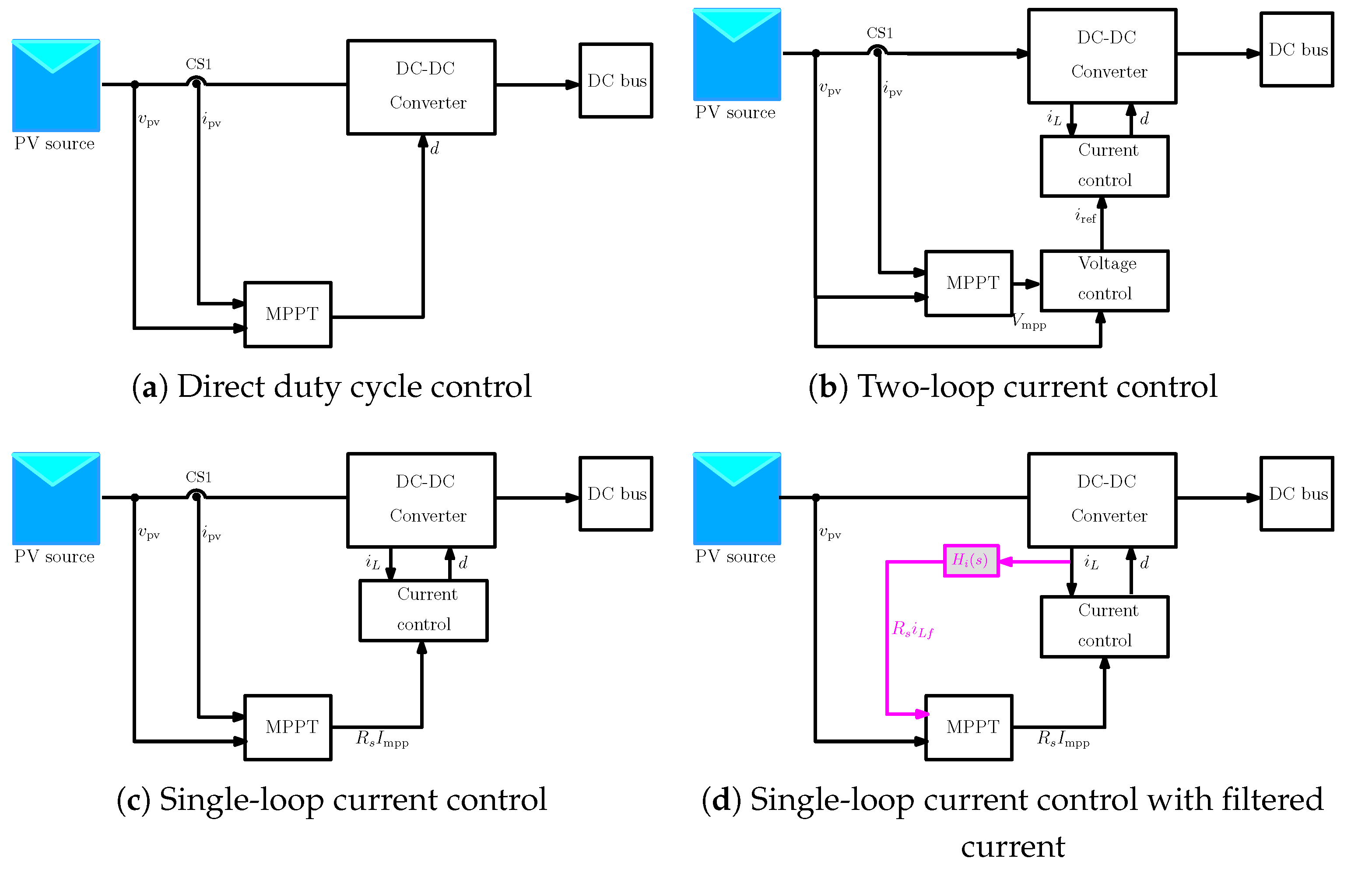
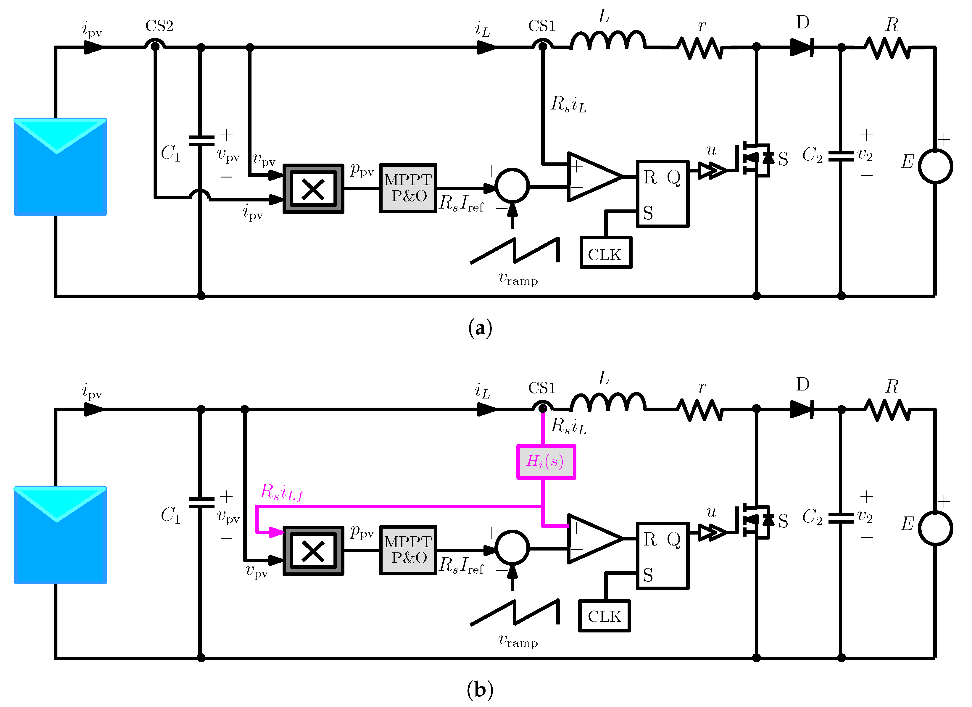
• Propose a flexible control based on the inductor current filtered by a low-pass filter integrating a relevant MPPT P&O algorithm to estimate the average value of the PV source power;
• Propose suitable orbital stability tools such as Floquet theory to study the stability of the overall system under consideration as a function of the cut-off frequency of the low-pass filter and the amplitude of the ramp signal;
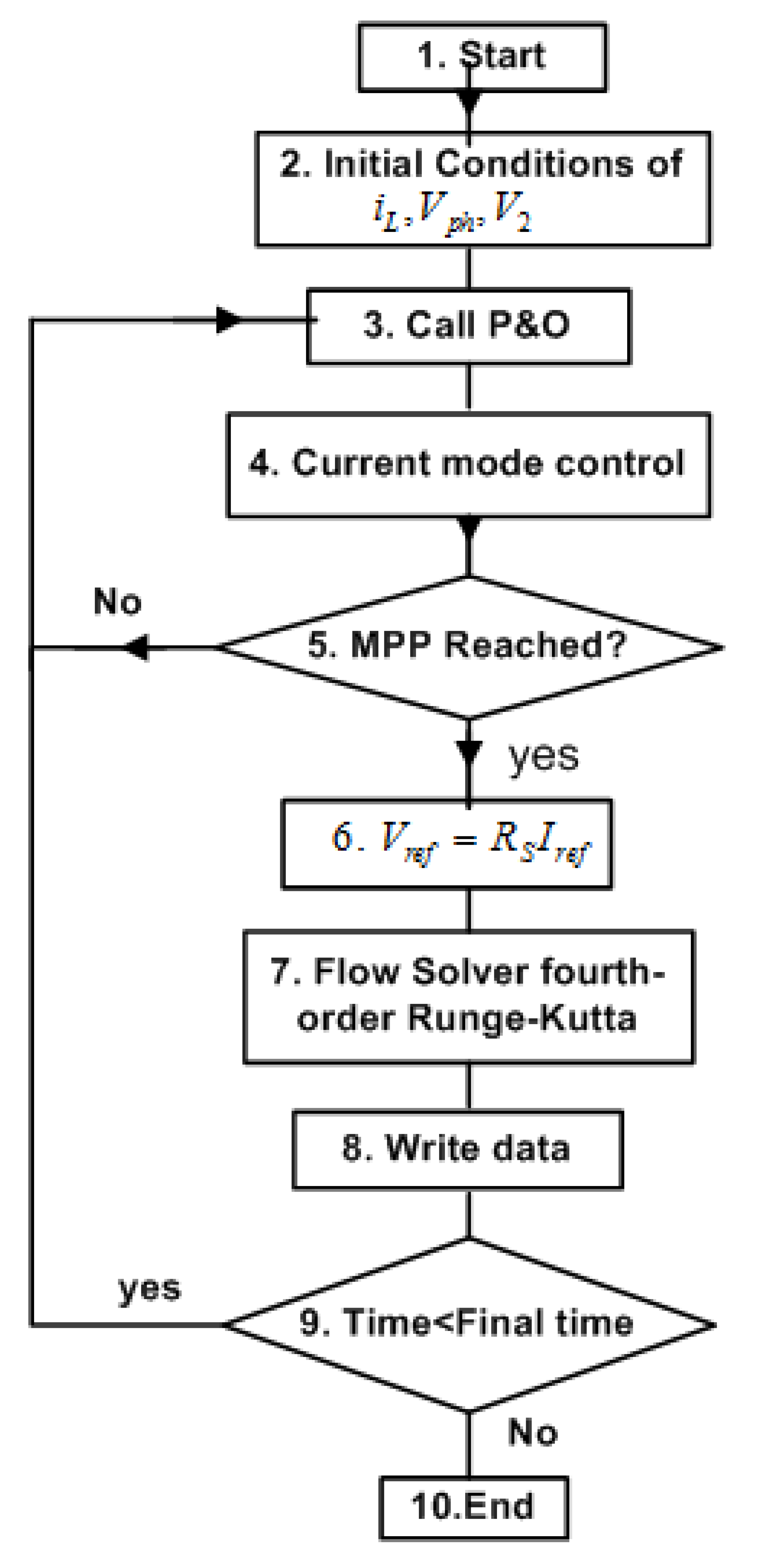
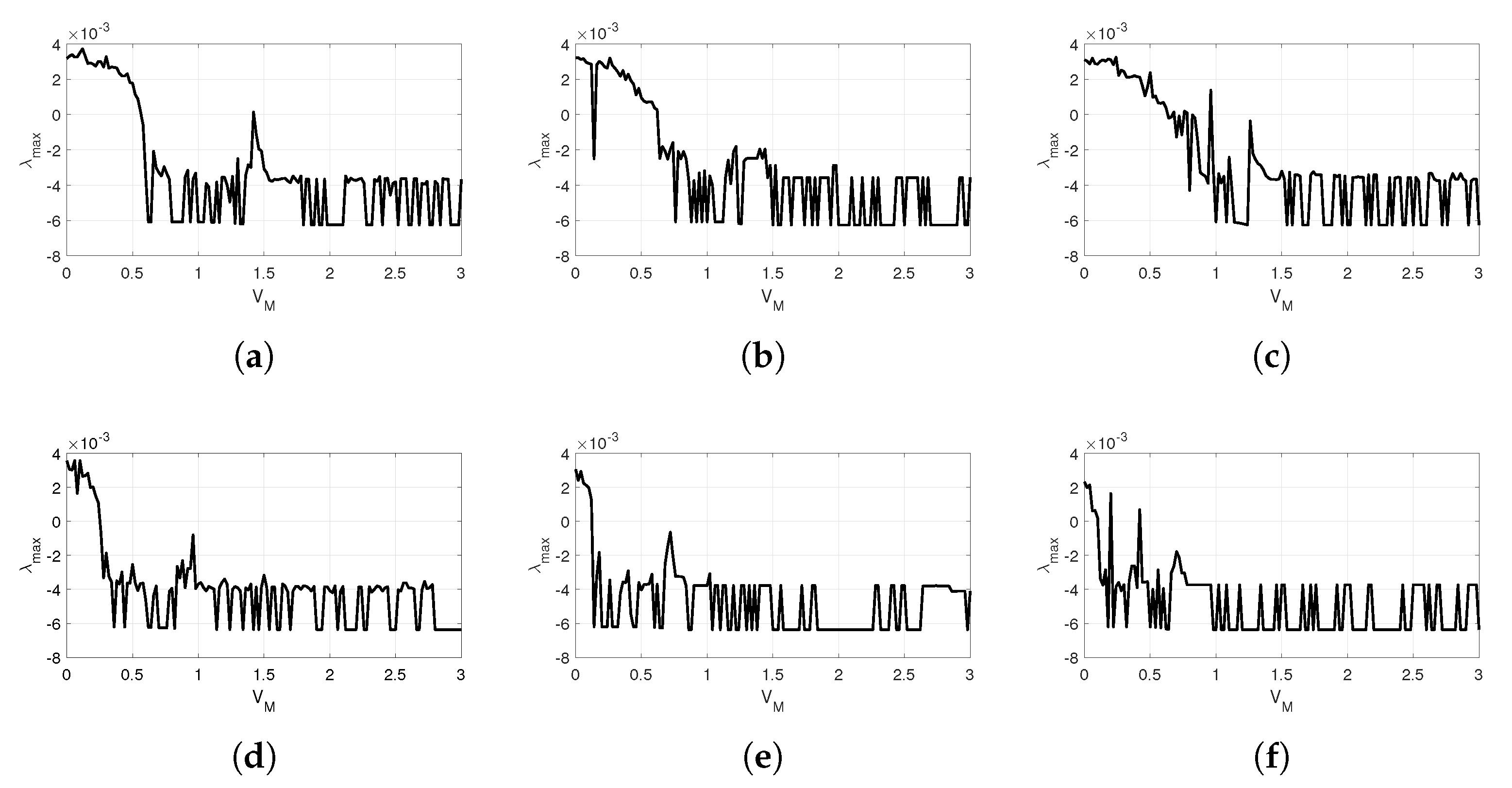
• Develop a bifurcation analysis of the DC-DC power system with MATLAB/SIMULINK based on the fourth-order Runge–Kutta numerical method for a deep study of the stability;
• Develop a bifurcation analysis of the DC-DC power system with the PSIM software that is close to experimental interpretation of the DC-DC system dynamic.

The rest of the paper is organized as follows: Section 2 presents materials and methods. Section 3 presents Results and Discussions and finally, concluding remarks are presented in Section 4.

2. Materials and Methods

2.1. System Evaluation

Let us consider the boost converter under current-mode control shown in Figure 2b. As far as the converter is concerned, it plays the role of an interface, for matching the energy flow between the source and the load [24]. The input capacitor with capacitance $C_1$ is used to smooth the voltage supplied by the PV to avoid ripples due to the nonlinearity of the PV generator. An LC filter is also used at the output to reduce switching ripples due to the switching nature of the converter and to provide a smooth output current to the DC output. Another function of our DC-DC converter is to track the maximum power point (MPP) by controlling the reference signal $R_s{i}_{\mathrm{ref}}$, using the perturbation and observation (P&O) algorithm, which increases or decreases the value of the reference signal $R_s{i}_{\mathrm{ref}}$ in order to position the PV operating point at its MPP at all times. The signal $R_s{i}_L$ is low-pass-filtered using $H_i\left(s\right)$ to obtain the signal $R_s{i}_{Lf}$, where $R_s$ is the sensor resistance. Considering a unity gain first-order filtering effect of the current sensor, the equation relating $i_{Lf}$ to $i_L$ in the Laplace domain is

$$\frac{I_{Lf}\left(s\right)}{I_L\left(s\right)}=\frac{{\omega }_c}{s+{\omega }_c},$$

(1)

where ${\omega }_c$ is the cut-off frequency of the filter. In time domain, this equation can be expressed as follows

$$\frac{d{i}_{Lf}}{dt}=-{\omega }_c{i}_{Lf}+{\omega }_c{i}_L.$$

(2)

The filtered signal $i_{Lf}$ is used both for current-mode control and for obtaining the average PV power after multiplying it by the PV voltage $v_{\mathrm{pv}}$. For current-mode control, the signal $R_s{i}_{Lf}$ is compared with the reference signal $R_s{I}_{\mathrm{ref}}-v_{\mathrm{ramp}}$, where $v_{\mathrm{ramp}}=m_{a}t\mathrm{mod}T$ is the ramp compensating signal, $m_a=V_M/T$ is its slope, $V_M$ is its amplitude and T is its period. The control logic compares the signal $R_s{i}_{Lf}$ with the signal $R_s{I}_{\mathrm{ref}}-v_{\mathrm{ramp}}$ in such a way that at the beginning of each switching cycle with the period dictated by the clock signal clk, the switch S is turned on and off whenever the signal $R_s{i}_{Lf}$ reaches the signal $R_s{I}_{\mathrm{ref}}-v_{\mathrm{ramp}}$. The binary signal u is a result of this switching decision and it takes the value 1 when the switch is turned on and 0 when it is turned off. The current reference $R_s{I}_{\mathrm{ref}}$ is provided by the MPPT.

A flowchart for current-mode control proposed in this work is shown in Figure 3. The program loop starts with the initialization of the voltage at the PV terminal, the current through the inductor and the voltage at the load (Block 2). These initial values are used to set the initial value of the reference voltage. In practice, the initial reference voltage is imposed by $V_{\mathrm{ref},\mathrm{init}}=0.85\times V_{\mathrm{MPPT},\max }$ [18]. Therefore, the choice of the initial values in the system must be made taking into account this condition on the reference voltage. When the irradiation is uniform, the P&O MPPT algorithm and CMC keep operating at the MPP (Block 3, Block 4, and Block 5). The P&O algorithm verifies fluctuations of power and voltage of PV array and determines the set-point voltage $V_{\mathrm{ref}}$ constantly. To maximize the output power from the PV array, its output voltage needs to be maintained at the level determined by the P&O algorithm. The resulting reference current $I_{\mathrm{ref}}$ from the reference voltage will produce the control signal that will be used by the pulse width modulation (PWM) for the boost converter switch. During the switching of the boost converter, the fourth-order Runge–Kutta algorithm is used to determine the dynamics taken by the converter (the values of the converter states and the values of the duty cycle) over time (Block 7, Block 8, Block 9). It should be noted that all numerical simulations in this paper are performed using MATLAB/SIMULINK. Other software such as C++, Fortran or Python could also be used because it is the simulation of ordinary differential equations [25,26,27,28,29].

2.2. Mathematical Modeling

Considering the system shown in Figure 2, applying Kirchhoff’s laws, we obtain the following system of equations:

$$\begin{array}{ccc}\hfill \frac{d{v}_{pv}}{dt}& =& \frac{i_{pv}}{C_1}-\frac{i_L}{C_1},\hfill \end{array}$$

(3)

$$\begin{array}{ccc}\hfill \frac{d{i}_L}{dt}& =& \frac{v_{pv}}{L}-\frac{r}{L}{i}_L-\frac{v_2}{L}\left(1-u\right),\hfill \end{array}$$

(4)

$$\begin{array}{ccc}\hfill \frac{d{v}_2}{dt}& =& \frac{E-v_2}{R{C}_2}+\frac{i_L}{C_2}\left(1-u\right),\hfill \end{array}$$

(5)

where $v_{pv}$ and $i_{pv}$ represent the voltage and current of the PV source, respectively. These two variables are related with a highly nonlinear and implicit Equation (3). $i_L$ is the current of the inductor, and u is the state of the switch. $C_1$ is the capacitance directly connected to the PV and its role is to smooth the voltage at the output of the PV. L represents the inductance, $V_{CC}$ the output voltage of the battery. r is the equivalent resistance in series with the coil and the equivalent resistance that can be felt at the output of the converter is R.

A PV generator represents a fundamental power source of a PV system. The output current/voltage characteristics depend on the solar irradiance and temperature. The PV generator has nonlinear electrical model with a single maximum power point (MPP). The performance of a PV generator is evaluated under standard test conditions, where the irradiance is normalized at 1 kW/m${}^2$ and the temperature is defined at 25 °C. A PV generator is characterized by its current–voltage characteristic (I–V) which can be subdivided into three operating zones, a linear zone with a practically constant current, a concave zone with almost constant voltage and an MPP which is the desired point for operation. Since this is the optimal point, the nonlinear characteristic (I–V) is linearized close to the MPP using Taylor’s series expansion and ignoring high-order terms. The (I–V) equation of the PV model can be approximated by the following linear Norton equivalent model [11]:

$${\widehat{i}}_{pv}\approx 2i_{mpp}-\frac{I_{\mathrm{mpp}}}{V_{\mathrm{mpp}}}{\widehat{v}}_{pv}+0\left({\widehat{v}}_{pv}^2\right).$$

(6)

Although numerical simulations could be performed using the nonlinear PV model, the linear model is useful to perform steady-state analysis, for controller design, stability analysis and for prediction of bifurcations. The state-space model of the power stage (3)–(5) together with (2) describing the current sensor and the switching logic determining the value of the binary control signal u appearing in (4) and (5) represent the closed-loop model of the PV system. While the nonlinear model of the PV generator can only be used for performing numerical simulations, the switched model with linearized PV generator model can be used for mathematically predicting the onset of period-doubling bifurcation in the system.

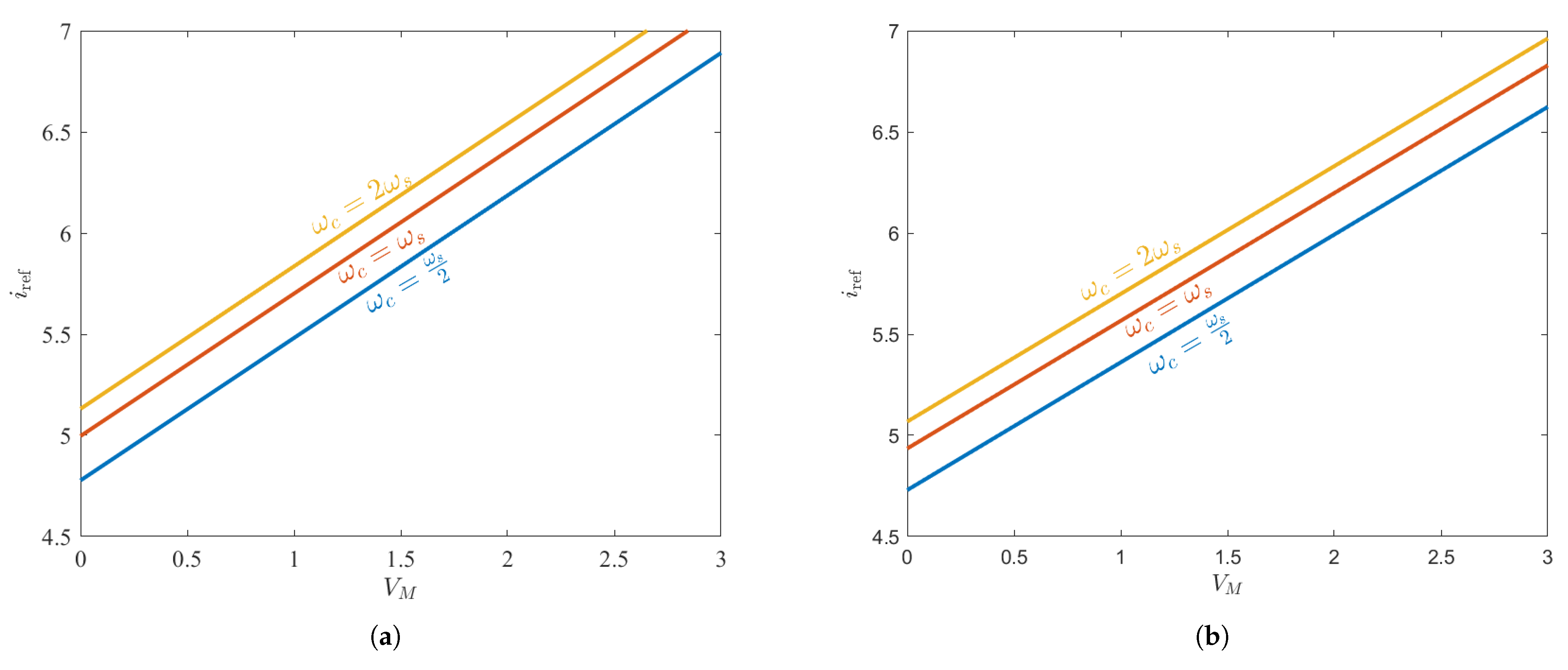
2.3. Steady-State Analysis

Obtaining the steady-state duty cycle D requires performing steady-state analysis. Under MPPT conditions and in steady-state operation, the following equalities hold

$$V_2(1-D)=V_{\mathrm{mpp}}-r{I}_{\mathrm{mpp}},V_2=E+R{I}_{\mathrm{mpp}}(1-D).$$

(7)

Solving both equations for the steady-state duty cycle D, one obtains

$$D=1-\frac{1}{2R{I}_{\mathrm{mpp}}}\left(\sqrt{4R{I}_{\mathrm{mpp}}(V_{\mathrm{mpp}}-r{I}_{\mathrm{mpp}})+E^2}-E\right).$$

(8)

Note that when the parasitic resistance r and R are negligible, one has which is the well-known expression of the duty cycle of an ideal boost converter with input $V_{\mathrm{mpp}}$ and output E. Since, under MPPT control and steady-state operation, the PV current will be equal to $I_{\mathrm{mpp}}$ and since the average capacitor voltage at the input port of the converter is zero, the inductor current average value in steady state will be also equal to $I_{\mathrm{mpp}}$. For this reason, the reference current under steady-state operation must be given by the following expression

$$I_{\mathrm{ref}}=I_{\mathrm{mpp}}+(\frac{m_a}{R_s}+\frac{m_1}{2})DT-\frac{1}{R_s}\frac{m_1(1-e^{-DT{\omega }_c})}{{\omega }_c},$$

(9)

where

$$m_1=\frac{V_{\mathrm{mpp}}-r{I}_{\mathrm{mpp}}}{L},m_a=\frac{V_M}{T}.$$

(10)

Note that if $m_a=0$ (no ramp compensation) and ${\omega }_c\to \infty$ (ideal current sensor), the previous expression becomes

$$i_{\mathrm{ref}}=I_{\mathrm{mpp}}+\frac{m_1}{2}DT=I_{\mathrm{mpp}}+\mathsf{\Delta }{i}_L,$$

(11)

where $\mathsf{\Delta }{i}_L=m_{1}DT/2$ is the ripple amplitude of the inductor current. Since $i_{\mathrm{ref}}$ is the peak value under the previous conditions, this guarantees that the average value of the inductor current will coincide with $I_{\mathrm{mpp}}$ in steady state and will also ensure the PV current in the sense of the average steady-state input capacitor current is zero.

Figure 4 shows the evolution of the reference current $i_{ref}$ in terms of the ramp amplitude $V_M$ and for two values of the output voltage E.

We notice from the above tables, that, whatever the value of ${\omega }_c$, the reference current increases with the amplitude of the ramp VM. Moreover, as ${\omega }_c$ increases, the curves $i_{ref}$ in terms of $V_M$ tend to be confused.

It is good to note that to maintain the same average inductor current and to make it equal to the MPP current, the current reference in the peak of the current loop control has been adapted according to (9).

2.4. Floquet Theory

2.4.1. The Piecewise Linear State-Space Switched Model Close to the Maximum Power Point

The periodic equation to be considered for our purposes will be expressed in the state-space representation (or matrix representation). This form lends itself well to the calculation of the solution of a differential equation system. The dynamics will be expressed as a function of a vector of variables, which we will call the state vector. Assuming that our subsystem is linear and time-invariant, the evolution of each subsystem is defined by:

$$\begin{array}{c}\dot{x}=A_{1}x+B_{1}W\mathrm{if}u=1,\hfill \\ \dot{x}=A_{0}x+B_{0}W\mathrm{if}u=0.\hfill \end{array}$$

(12)

where $x={\left(x_1{x}_2{x}_3{x}_4\right)}^T$, $A_1,B_1,A_0,B_0$ are the state and input matrices corresponding to the different switch states and the external input parameters vector are given by:

$$A_1=\left(\begin{array}{cccc}-\frac{1}{R_{pN}{C}_1}& -\frac{1}{C_1}& 0& 0\\ \frac{1}{L}& -\frac{1}{L}r& 0& 0\\ 0& 0& -\frac{1}{R{C}_2}& 0\\ 0& w_c{k}_p& 0& -w_c\end{array}\right),$$

(13)

$$A_0=\left(\begin{array}{cccc}-\frac{1}{R_{pN}{C}_1}& -\frac{1}{C_1}& 0& 0\\ \frac{1}{L}& -\frac{1}{L}r& -\frac{1}{L}& 0\\ 0& \frac{1}{C_2}& -\frac{1}{R{C}_2}& 0\\ 0& w_c{k}_p& 0& -w_c\end{array}\right),$$

(14)

$$B_1=\left(\begin{array}{cc}\frac{2}{C_1}& 0\\ 0& 0\\ 0& \frac{1}{R{C}_2}\\ 0& 0\end{array}\right),$$

(15)

$$B_0=\left(\begin{array}{cc}\frac{2}{C_1}& 0\\ 0& 0\\ 0& \frac{1}{R{C}_2}\\ 0& 0\end{array}\right),$$

(16)

$$W=\left(\begin{array}{c}{i}_{mpp}\\ E\end{array}\right).$$

(17)

The switching condition in Figure 2 is given by:

$$h(x,t)=R_s\left(i_{ref}-Kx\right)-\frac{V_M}{T}t,$$

(18)

with $\frac{V_M}{T}t=V_{ramp}$, the vector K is given by:

$$K={\left(\begin{array}{c}0\\ 0\\ 0\\ -1\end{array}\right)}^T.$$

(19)

2.4.2. Stability Analysis Using Floquet Theory

The differential equations describing the dynamics of switching converters are time-periodic with the switching period T determining the periodicity of solutions at the fast switching scale. Floquet theory has been widely used in the analysis of the stability of dynamical systems [30] in general and in switching converters in particular [11,31,32]. For DC-DC converters, the stability dynamics at the fast switching cycle can be accurately predicted by analyzing the stability of the fixed points of the Poincare map of the system using its Jacobian matrix or using Floquet theory combined with the Filippov method which leads to the same results as the Poincare map [33]. The main tool for studying the stability of periodic orbits using Floquet theory is the principal fundamental matrix or the monodromy matrix M. This matrix plays a key role in the accurate stability analysis of switching systems [34,35,36]. The dynamics in the vicinity of a quasi-static periodic orbit can be expressed in the monodromy matrix as follows:

$$\widehat{x}(t+T)=M\widehat{x}\left(t\right)\forall t,$$

(20)

where the overhat stands for small signal variations. Its eigenvalues are called the characteristic multipliers or Floquet multipliers and it can be seen that they determine the amount of contraction or expansion near a periodic orbit and hence they determine the stability of these periodic orbits. It can be obtained by computing the state transition matrices before and after each switch and the saltation matrix that describes the behaviors of the solution 7 switching [24] which are described in the following.

Let $X\left(DT\right)={\left(I-\mathrm{\Phi }\right)}^{-1}\mathrm{\Psi }$ be the steady-state value of X at time instant $DT$, where $\mathrm{\Phi }={\mathrm{\Phi }}_1{\mathrm{\Phi }}_0,{\mathrm{\Phi }}_1=e^{A_{1}DT},{\mathrm{\Phi }}_0=e^{A_0(1-D)T}$,

$$\mathrm{\Psi }=e^{A_{1}DT}{A_0}^{-1}\left(e^{A_0\left(1-D\right)T}-I\right)B_{0}W+{A_1}^{-1}\left(e^{A_{1}DT}-I\right)B_{1}W.$$

(21)

The monodromy matrix use [11] can be expressed as follows $P={\mathrm{\Phi }}_{0}S{\mathrm{\Phi }}_1$

$$P={\mathrm{\Phi }}_{0}S{\mathrm{\Phi }}_1,$$

(22)

where S is saltation matrix and is given by:

$$S=I+\frac{\left(A_{0}X\left(DT\right)-A_{1}X\left(DT\right)\right)K^T}{K^T\left(A_{1}X\left(DT\right)+B_{1}W\right)+m_a}.$$

(23)

Equations (22) and (23) will allow us to determine the Floquet multipliers. According to Floquet’s theory, if only one multiplier has a value equal to −1, then the dynamics of the system presents period doubling bifurcation. In general, the occurrence of the critical point of this bifurcation has two regions: a region of subharmonic oscillation and a region of periodic oscillation of period-1. The second region described above is the stability region in power systems [24].

3. Results and Discussions

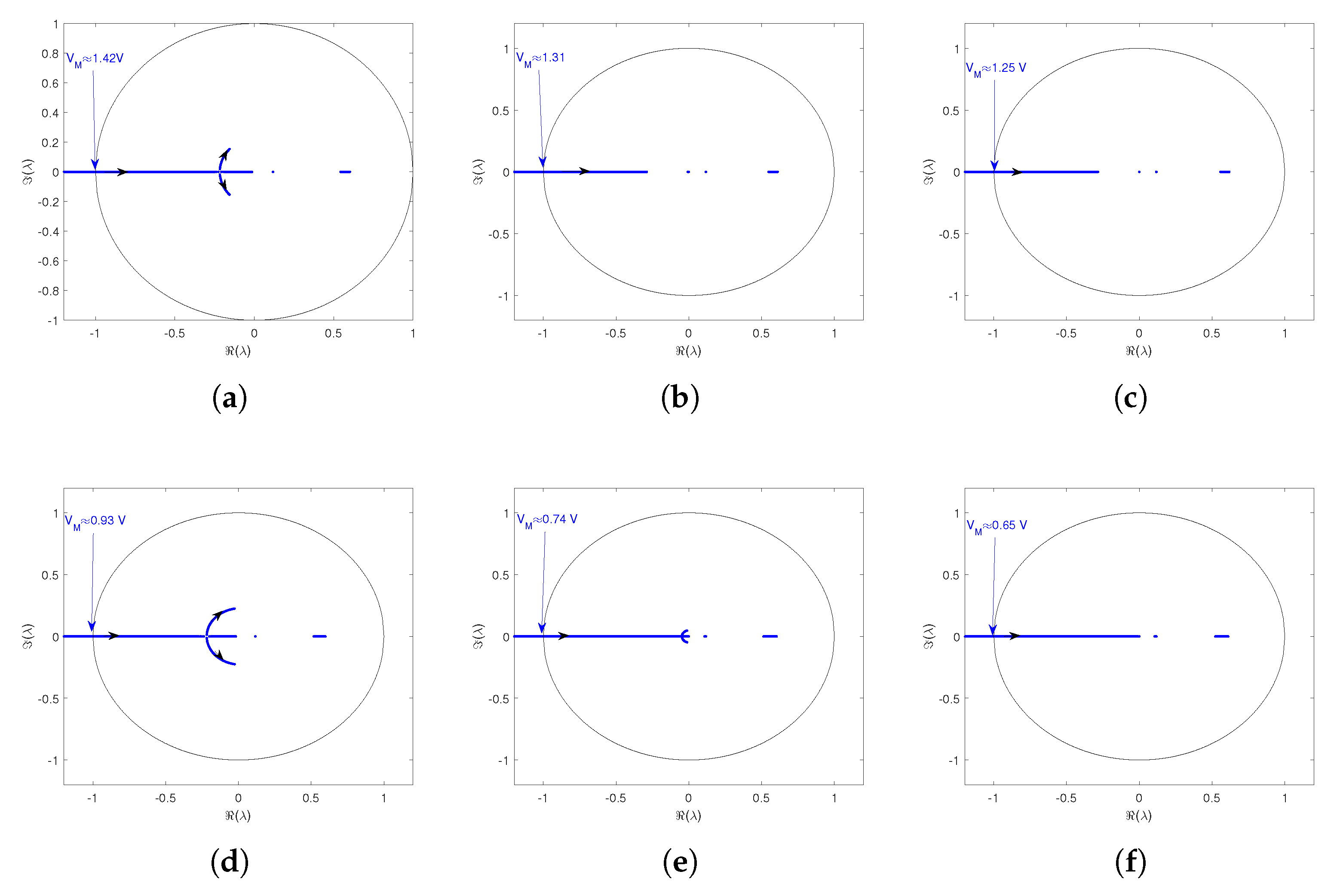
3.1. Floquet Theory on the Stability

3.1.1. Simulations Results in MATLAB/SIMULINK Software

The monodromy matrix is explained in Equation (23). Using a code developed in the MATLAB software, we find the eigenvalues noted as $\lambda$ of this monodromy matrix. These eigenvalues are solutions of equation $det(P-\lambda I)=0$. Figure 5 is the representation in the complex plane of the Floquet multipliers when the amplitude $V_M$ varies from 0.0 to 3, for three values of the cut frequency $f_c=\frac{f_s}{2},f_c=f_s,f_c=2f_s\mathrm{with}{f}_s=50\mathrm{kHz}$ and for two values of the output voltage $\left(E=60\mathrm{V}\mathrm{and}E=48\mathrm{V}\right)$. It should be noted that the period-1 orbit will lose stability and bifurcate into period-2 (sub-harmonic oscillation) if the system has the phenomenon of smooth period-doubling when a control parameter varies. Moreover, at this value of the control parameter, period-1 is destroyed and period-2 is created. Indeed, one of the Floquet multipliers is approximately equal to 1, which allows us to say that at this value of the amplitude $V_M$ the period-1 orbit destabilizes and gives way to a sub-harmonic oscillation of period 2. In Figure 5, the followings remarks can be noticed:

Remark 1.

We find that for several values of the gain $V_M$, the moduli of the Floquet multipliers are located in the circle of unit radius synonymous with the stability of the period-1 orbit. In addition, for other ranks of the parameter $V_M$, the Floquet multipliers are located outside the circle of unit radius, which is synonymous with destabilization of the periodic orbit of period-1.

Remark 2.

We observe that when for $E=60\mathrm{V}$, $E=48\mathrm{V}$, $f_c$ is increasing, i.e., $\left(f_c=\frac{f_s}{2}\right)<\left(f_c=f_s\right)<\left(f_c=2f_s\right)$, the critical values $V_M$ (allowing us to set the boundary between period-1 oscillations and subharmonic oscillations) evolve in a decreasing manner, i.e., $V_{M_{\frac{f_s}{2}}}>V_{M_{f_s}}>V_{M_{2f_s}}$. We can conclude that the stability zone increases with the cut-off frequency, this conclusion justifies once again the bifurcation diagrams in Figure 6.

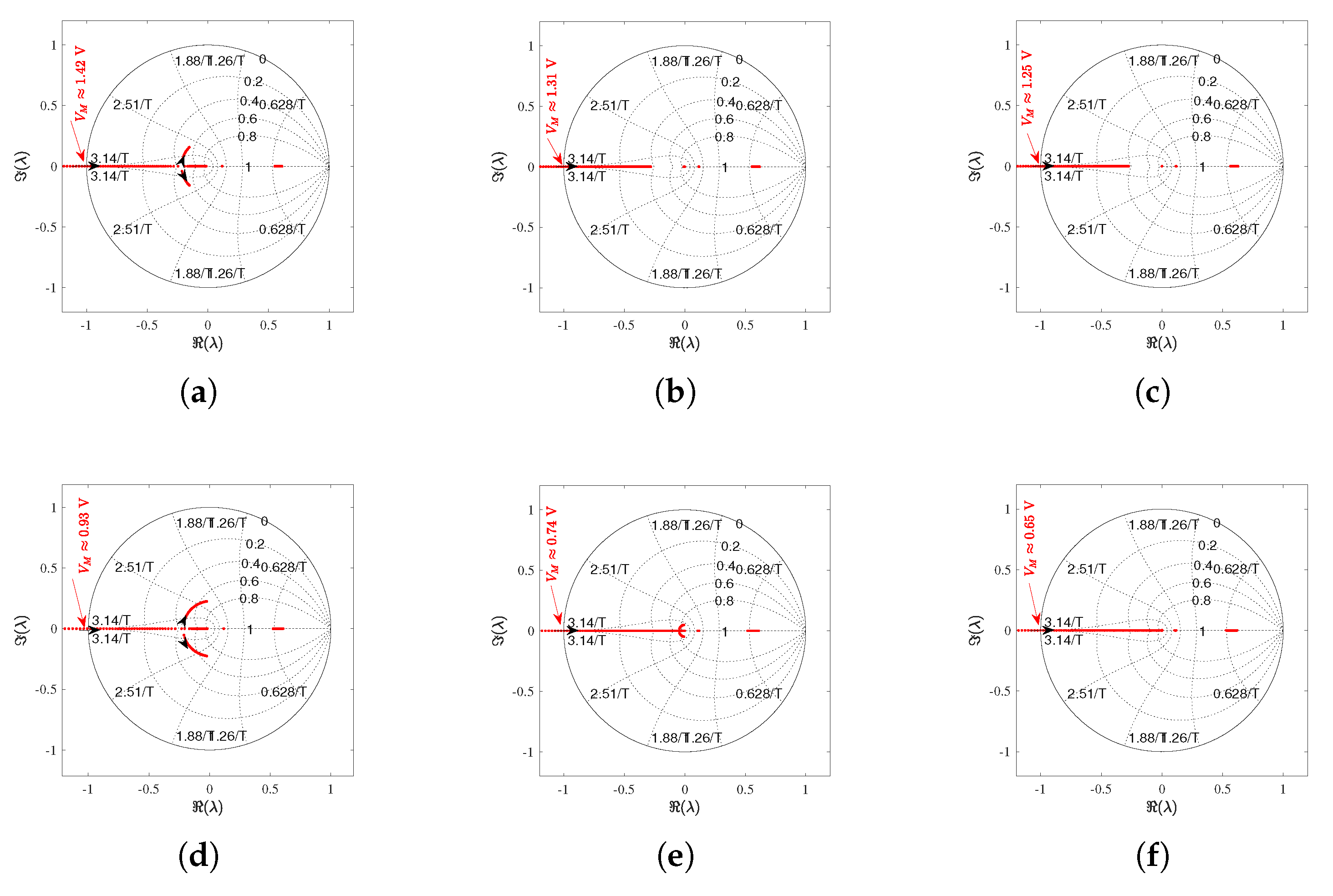
3.1.2. Simulations Results in PSIM Software

Figure 7 shows the results of the stability study of our system in the PSIM software. The PSIM software is a power electronics simulation software. We notice a similarity between the results obtained with PSIM and those obtained with MATLAB/SIMULINK. In the following, we will use the bifurcation diagrams for a more detailed study.

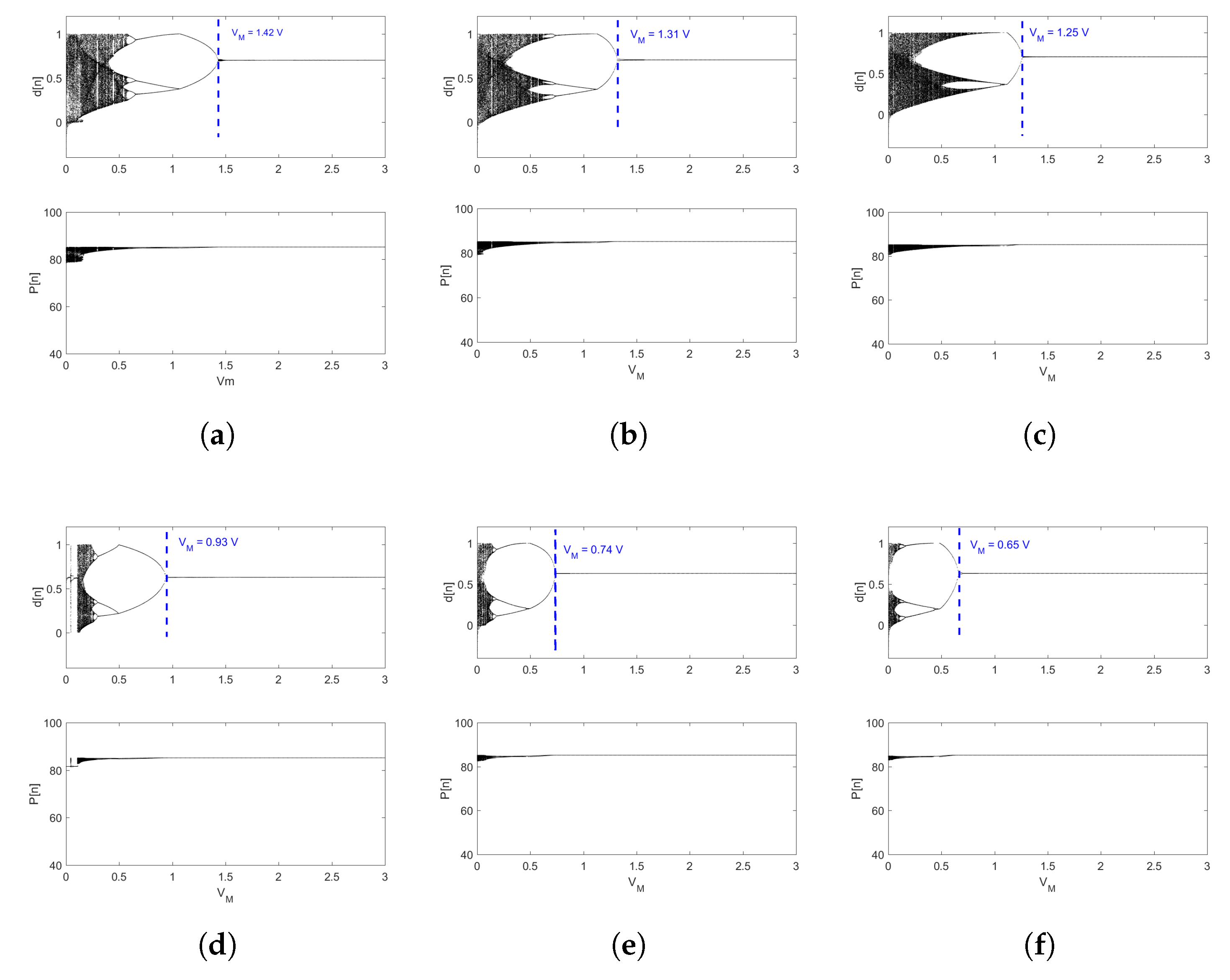
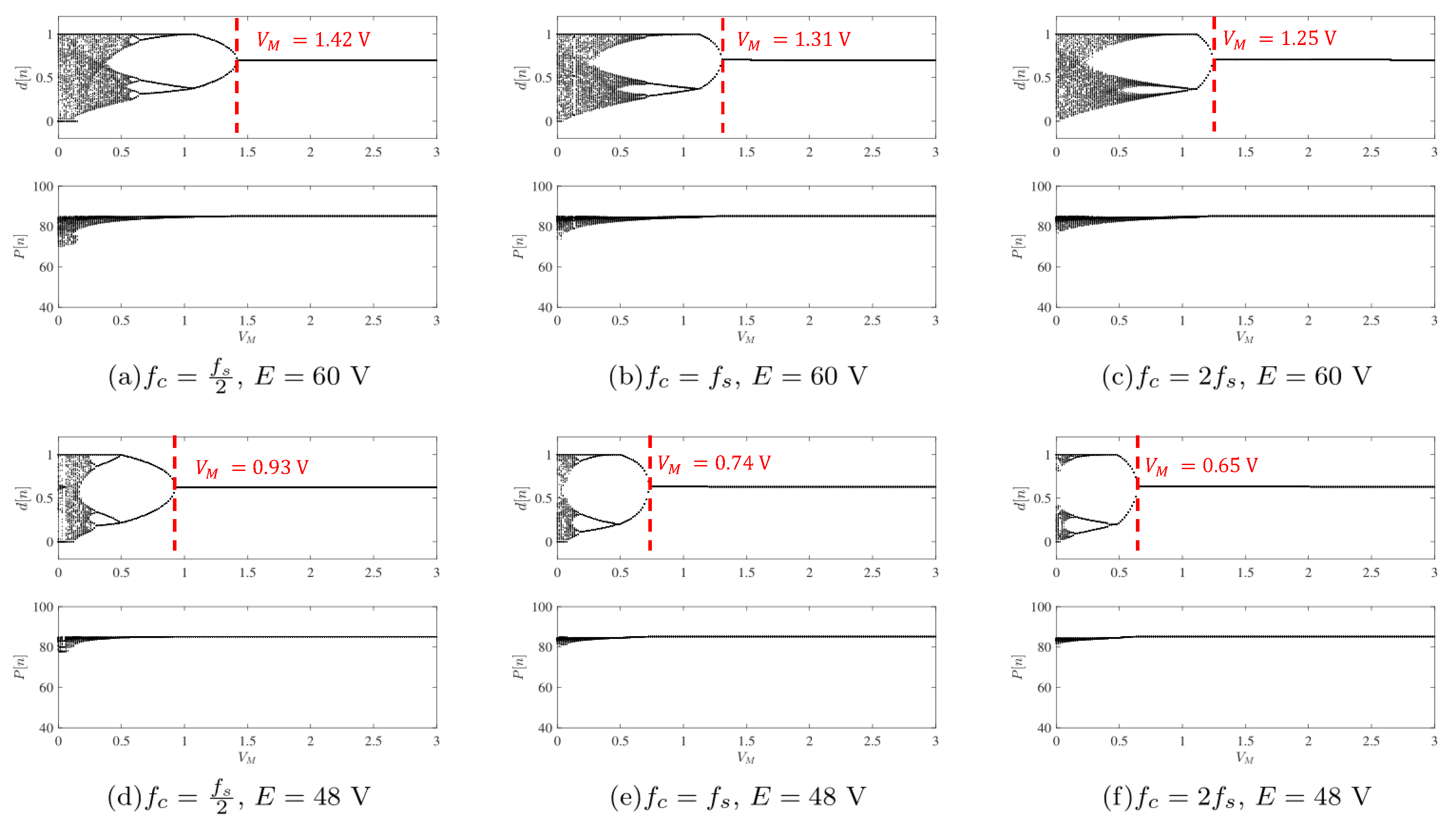
3.2. Bifurcation Behavior from the Nonlinear Circuit-Level Switched Model with the Linear Model of the PV Generator from MATLAB/SIMULINK Software

Bifurcation diagrams constitute appropriate means of recapitulating different transitions to chaos in the system in terms of different parameter values. The maximum Lyapunov exponent is complementary with bifurcation diagram, it is the tool that allows us to conclude if the system is chaotic or not and there are computed following the well-known Wolf algorithm [37]. In this section, the numerically dynamics behavior of our system is performed in MATLAB/SIMULINK software by integrating system (3) using the most frequent fourth-order Runge–Kutta scheme [38] adapted to DC-DC converters which offers a better accuracy for solving single-step differential equations unlike the discretization method developed in the literature. First, the system has been carefully studied through simulations using the linear model of the PV generator in MATLAB software. We used a fixed time step equal to $h=5\times {10}^{-8}$, a total number of iterations $N={10}^6$ and a transient phase-cut to $N^{\prime }=8\times {10}^5$ The bifurcation diagram and graphs of maximal Lyapunov exponents presented below are obtained for three values of the cut-off frequency, i.e., $f_c=\frac{f_s}{2},f_c=f_s,f_c=2f_s\mathrm{with}{f}_s=50$ kHz, and for two values of DC output voltage $\left(E=60\mathrm{V}\mathrm{and}E=48\mathrm{V}\right)$, we use ramp amplitude $V_M$ as a bifurcation parameter. The local maximas of the duty cycle and the local maximas of the output power of the generator made it possible to plot bifurcation diagrams. The dynamics of the MPPT algorithm is neglected because it is usually much slower than the converter dynamics. The values of the parameters used for this study are shown in

Table 1. Boost converter parameters.

Parameters	Values
$C_1$	10 $\mu$F
L	200 $\mathsf{\mu }$H
r	100 m$\mathsf{\Omega }$
E	48 V and 60 V
$R_2$	200 m$\mathsf{\Omega }$
$R_s$	1 $\mathsf{\Omega }$
$C_2$	47 $\mathsf{\mu }$F
$i_{\mathrm{ref}}$	updated according to (9)
$f_s$	50 kHz
$f_c$	variable
$V_M$	Variable

and

Table 2. Parameter of the PV generator (BP 585 module).

Parameters	Values
Maximum power $P_{\mathrm{mpp}}$	85.17 W
Voltage at maximum power $V_{\mathrm{mpp}}$	18.28 V
Current at maximum power $V_{\mathrm{mpp}}$	4.66 A
Maximum power $P_{max}$	85.17 W
Short-circuit current $I_{sc}$	5 A
Open-circuit voltage $V_{oc}$	$21.1$ V

.

Figure 6 shows the bifurcation diagrams when the $V_M$ parameter varies for different values of cut-off frequency and output voltage. For $E=60\mathrm{V}\mathrm{and}\left(f_c=\frac{f_s}{2},f_c=f_s,f_c=2f_s\right)$, we can observe in Figure 6a–c inverse period-doubling phenomena from chaos to period-1 chaos $\to period-8\to period-4\to period-2\to period-1$ and when the ordinate axis is a representation of the local maxima of the duty cycle. For a representation of the local maxima of the power output of pv on the ordinate axis of the same figure Figure 3$(a_1,b_1,c_1)$ show that we start directly from chaos in period-1, we also remark that the system stabilizes at the maximum power point, which shows that our MPPT controller used is good. In the same figure, we can see that when the cut-off frequency increases, i.e., $\left(f_c=\frac{f_s}{2}\right)<\left(f_c=f_s\right)<\left(f_c=2f_s\right)$ the critical value $V_M$ represents the boundary between the periodic oscillations of period-1 and the subharmonic oscillations decrease. In other words, when the cut-off frequency increases, the system tends to lose its subharmonic behaviour. Thus, the cut-off frequency increases with the stability range, which is interesting for this study since the desired behavior for a pv energy conversion chain is the periodic behavior.

For $E=48\mathrm{V}\mathrm{and}{f}_c\in \left(\frac{f_s}{2},f_s,2f_s\right)$, Figure 3$(d_1,e_1,f_1)$, we can also observe inverse period-doubling phenomena from chaos to period 1 and a faster loss of chaos. We can, therefore, conclude in this part that it is desirable to choose $E=48\mathrm{V}$ as the output voltage of the battery instead of $E=60\mathrm{V}$ because it is at this value and for different values of the cut-off frequency that the system tends to quickly lose subharmonic behaviors since the desire behavior for this type of application is the periodic behavior.

Figure 8 shows the Lyapunov exponent graphs complementary with the bifurcation diagrams in Figure 6. These graphs are obtained for three values of the cut-off frequency and for two values of the output voltage and in the $V_M$ zone between $0\le V_M\le 1$, in this area, we observe in Figure 8 negative values of the maximum Lyapunov exponent which correspond to regular oscillations in the system and positive values corresponding to subharmonic oscillations. We can also remark that the cut-off frequency increases with stability, which justifies the bifurcation diagrams of Figure 8.

The bifurcation diagrams Figure 6 and Lyapunov exponent in Figure 8 show an overlap between regular and irregular behaviors in the subharmonic oscillation zone. In addition, the bifurcation diagrams in Figure 6 show border collision [39,40,41] respectively to the critical values $V_M=1.42\mathrm{V},V_M=1.31\mathrm{V},V_M=1.25\mathrm{V}$ (see Figure 6a–c) and $V_M=0.93\mathrm{V},V_M=0.74\mathrm{V},V_M=0.65\mathrm{V}$ (see Figure 6d,e,f).

Remark 3.

We note that for $E=60\mathrm{V}$, the critical values $V_M$, Figure 6a–c, are superior to those of $E=48\mathrm{V}$ Figure 6d–f; this means that the range of stability is greater when $E=48\mathrm{V}$ compared with $E=60\mathrm{V}$. Therefore, it is desirable to choose E = 48 V as the battery output voltage instead of E = 60 V because it is at this value and for different values of the cut-off frequency that the system tends to quickly lose the subharmonic behaviours and increases the stability range.

3.3. Bifurcation Behavior from the Nonlinear Circuit-Level Switched Model with the Nonlinear Model of the PV Generator from PSIM Software

The circuit diagram for the current-mode-controlled boost converter is constructed using the PSIM simulation software. The selection of component parameters is consistent with the numerical simulation in Table 1 and Table 2. In this part, nonlinear phenomena such as bifurcations are exhibited, using the nonlinear and linear models of the PV generator, the $V_M$ bifurcation parameter, the different values of the output voltage $\left(E=60\mathrm{V}\mathrm{and}E=48\mathrm{V}\right)$ and the different values of the cut-off frequency $f_c=\frac{f_s}{2},f_c=f_s,f_c=2f_s\mathrm{with}{f}_s=50$ kHz being equal to those used in numerical simulations in MATLAB. Comparing the simulation bifurcation of the nonlinear model of the pv generator in Figure 9 ( PSIM simulation) with that in Figure 6 (MATLAB simulation), it can be seen that the results are in almost perfect agreement.

Note here that the results presented in these two figures are identical, for example, for E = 60 and $\left(f_c=\frac{f_s}{2}\right)$, the critical value obtained is the same in both cases and is equal to $V_M=1.42\mathrm{V}$. We want to show through these two graphs that linearizing appropriately the PV generator model does not affect the accuracy of the model in predicting the period-doubling bifurcation of the system. The aim is to study the linear model of PV generator, which is going to help us to study the stability of our system, as it is very difficult to study stability with the nonlinear model of PV.

Remark 4.

Figure 9 shows the bifurcation with the nonlinear model of the PV generator substituted by its linearized model constituting a linear resistance $V_{\mathrm{mpp}}/I_{\mathrm{mpp}}$ and a current source $2I_{\mathrm{mpp}}$. It can be observed that the matching between these bifurcation diagrams and those obtained in Figure 6 is excellent. It is widely believed among the power electronics community that with values of steady-state duty cycles of less than 0.5, no external ramp is needed to achieve a stable system. However, from the previous bifurcation diagrams, it is clear that the system is still prone to period-doubling bifurcation even for $D<0.5$ if the cut-off frequency of the current sensor is relatively low. Therefore, a ramp slope compensation is also necessary for duty cycle values less than $0.5$.

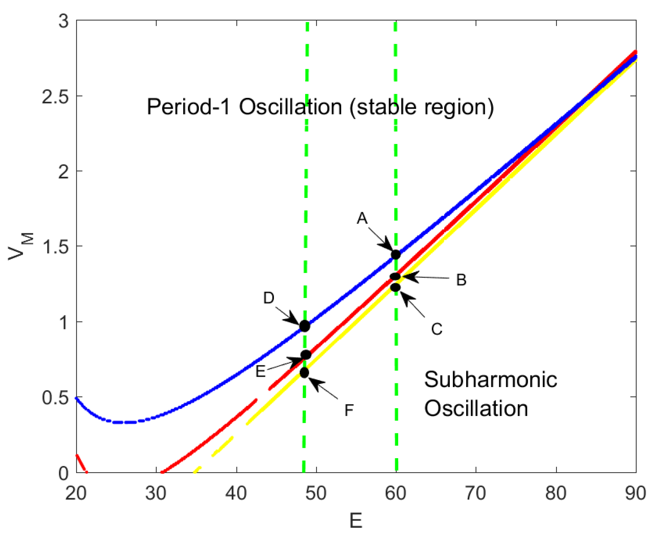
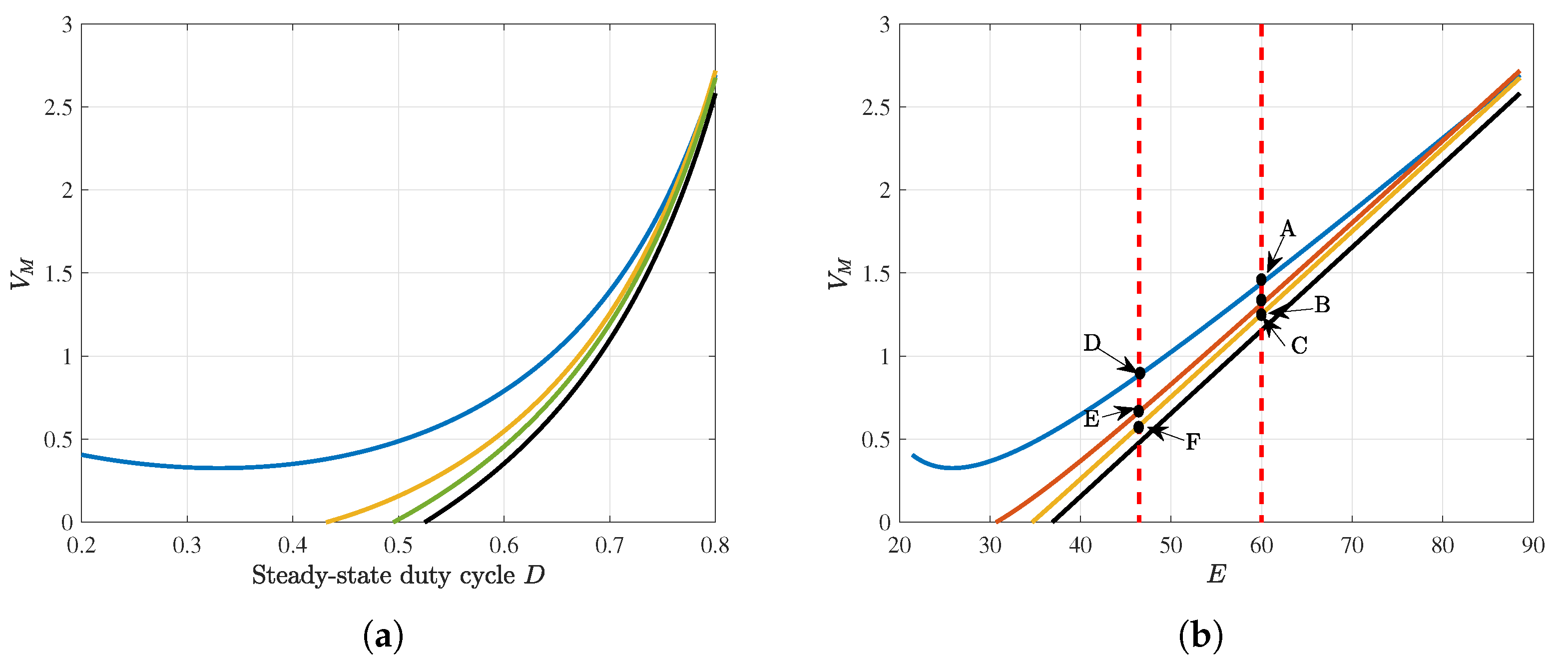
3.4. Stability Boundaries in the Parameter Space

Now that the nonlinear behaviour of the PV system under peak current-mode control is understood and the mechanisms of losing stability are known, the stability boundary for useful practical design will be determined.

The focus of this paper is on the period-doubling bifurcation boundary. The results helps in setting the design parameters as they show the stable region in the parametric space.

One of the ways to locate the subharmonic oscillation boundary is by using the expression of the characteristic equation $det(\mathbf{P}-\lambda \mathbf{I})=0$, imposing the period-doubling condition in the eigenvalue $\lambda$ and solving the resulting equation together with the steady-state condition. Therefore, at the boundary of this bifurcation, the following conditions hold

$$\begin{array}{c}\hfill det(\mathbf{P}+\mathbf{I})=0,\end{array}$$

(24a)

$$\begin{array}{c}\hfill \mathbf{x}\left(DT\right)-\mathbf{x}\left(\right(D+1\left)T\right)=\mathbf{0},\end{array}$$

(24b)

where $\mathbf{0}\in {\mathbb{R}}^4$ is a null vector. Note that the integral state variable can be determined by (24b).

Figure 10 presents the stability study in two dimensions of the photovoltaic system obtained in MATLAB/SIMULINK. It clearly shows the regions of stability (period-1 oscillations) and instability (subharmonic oscillations) of the system in the E-plane for three values of the cut-off frequency: blue $f_c=f_s/2$, red $f_c=f_s$ and yellow $f_c=2f_s$. The other system parameters are taken as in Table 1 and Table 2. We see on this map that when $20\mathrm{V}\le E\le 30\mathrm{V}$, the system does not show period-doubling phenomenon except for $f_c=f_s/2$. In this case, this map is not sufficient to conclude on the system stability. Moreover, for $30\mathrm{V}\le E\le 70\mathrm{V}$, the stability domain of the photovoltaic system increases with the filter cut-off frequency. Finally, for $70\mathrm{V}\le E\le 90\mathrm{V}$, the filter cut-off frequency has no influence on the stability of the PV system. These results are more complete than the results obtained in the previous sections, so this map will be a crucial tool in the decision-making process for engineers in industries.

Figure 11a shows the critical curves in the plane $D-V_M$ for different values of $f_c$. The conventional boundary with ${\omega }_c\to \infty$ is also shown. Figure 11b shows the critical curves in the plane $E-V_M$ for different values of $f_c$. The critical points for $E=48$ and $E=60$ are indicated in the figure. The critical values of the ramp amplitude for the different values of E and $f_c$ remarkably coincide with the critical values obtained by the bifurcation diagrams in the previous section. For instance, for point A, one has $E=60$ V and $f_c=f_s/2$ and the critical point of $V_M$ is $1.42$ V agreeing with the bifurcation diagram of Figure 6a. Above the curves, the system is stable and below it, it exhibits period-doubling bifurcation. The critical curve in the plane $D-V_M$ passes very close to the point $(0,\frac{1}{2})$ as long as $f_c$ is relatively small. This curve becomes concave in this plane when $V_M$ is increased. By increasing the ramp amplitude $V_M$, the region of stability is widened for $D>\frac{1}{2}$ and is reduced for $D<\frac{1}{2}$. Furthermore, the stable region becomes wider when increasing the cut-off frequency. These last results obtained with PSIM software are in perfect agreement with those of Figure 10 obtained with MATLAB/SIMULINK software.

4. Conclusions

This paper focuses on the nonlinear behaviour and stability of the current-mode-controlled boost converter with the battery load. First, numerical analysis of its state equations, bifurcation diagrams and Lyapunov exponent was conducted in MATLAB/SIMULINK Software using a linear model of PV. Secondly, analogy simulations using PSIM were performed using a nonlinear models of the PV generator. The stability of a boost converter supplied by a PV panel was studied. To make an analytical study possible, the nonlinear PV generator has been linearizing around its MPPT. The simulation results considered three values of the cut-off frequency and two values of the output voltage. They showed through the bifurcation diagrams and the Lyapunov exponent that the system presents nonlinear phenomena such as chaos and periodic motion, which are influenced by system parameters and topological structure. The numerical results obtained in MATLAB/SIMULINK software are remarkable in their agreement with the analogy simulations in PSIM. We can also mention that linearizing appropriately the PV generator model does not affect the accuracy of the model in predicting the period-doubling bifurcation of the system. In general, we have seen that the stability increases with the frequency of the cut which is interesting about this study since the type of behaviour desired for a PV is the period-1.

References

1. Srinivasarao, P.; Peddakapu, K.; Mohamed, M.; Deepika, K.K.; Sudhakar, K. Simulation and experimental design of adaptive-based maximum power point tracking methods for photovoltaic systems. Comput. Electr. Eng. 2021, 89, 106910. [Google Scholar] [CrossRef]
2. Kishore, D.K.; Mohamed, M.; Sudhakar, K.; Peddakapu, K. Swarm intelligence-based MPPT design for PV systems under diverse partial shading conditions. Energy 2023, 265, 126366. [Google Scholar] [CrossRef]
3. Kishore, D.K.; Mohamed, M.; Sudhakar, K.; Peddakapu, K. An improved grey wolf optimization based MPPT algorithm for photovoltaic systems under diverse partial shading conditions. Proc. J. Phys. Conf. Ser. 2022, 2312, 012063. [Google Scholar] [CrossRef]
4. Syafiq, A.; Pandey, A.; Adzman, N.; Abd Rahim, N. Advances in approaches and methods for self-cleaning of solar photovoltaic panels. Sol. Energy 2018, 162, 597–619. [Google Scholar] [CrossRef]
5. Bourourou, F.; Tadjer, S.A.; Habi, I. Wind Power Conversion Chain Harmonic Compensation using APF Based on FLC. Alger. J. Renew. Energy Sustain. Dev. 2020, 2, 75–83. [Google Scholar] [CrossRef]
6. Rana, K.; Kumar, V.; Sehgal, N.; George, S.; Azar, A.T. Efficient maximum power point tracking in fuel cell using the fractional-order PID controller. In Renewable Energy Systems; Azar, A.T., Kamal, N.A., Eds.; Advances in Nonlinear Dynamics and Chaos (ANDC); Academic Press: Cambridge, MA, USA, 2021; pp. 111–132. [Google Scholar]
7. Fekik, A.; Azar, A.T.; Kamal, N.A.; Serrano, F.E.; Hamida, M.L.; Denoun, H.; Yassa, N. Maximum Power Extraction from a Photovoltaic Panel Connected to a Multi-cell Converter. In Proceedings of the International Conference on Advanced Intelligent Systems and Informatics, Cairo, Egypt, 19–21 October 2020; Hassanien, A.E., Slowik, A., Snášel, V., El-Deeb, H., Tolba, F.M., Eds.; Springer International Publishing: Cham, Switzerland, 2021; pp. 873–882. [Google Scholar]
8. Ammar, H.H.; Azar, A.T.; Shalaby, R.; Mahmoud, M.I. Metaheuristic Optimization of Fractional Order Incremental Conductance (FO-INC) Maximum Power Point Tracking (MPPT). Complexity 2019, 2019, 1–13. [Google Scholar] [CrossRef]
9. Amara, K.; Malek, A.; Bakir, T.; Fekik, A.; Azar, A.T.; Almustafa, K.M.; Bourennane, E.B.; Hocine, D. Adaptive neuro-fuzzy inference system based maximum power point tracking for stand-alone photovoltaic system. Int. J. Model. Identif. Control 2019, 33, 311–321. [Google Scholar] [CrossRef]
10. Ben Smida, M.; Sakly, A.; Vaidyanathan, S.; Azar, A.T. Control-Based Maximum Power Point Tracking for a Grid-Connected Hybrid Renewable Energy System Optimized by Particle Swarm Optimization. In Advances in System Dynamics and Control; Azar, A.T., Vaidyanathan, S., Eds.; Advances in Systems Analysis, Software Engineering, and High Performance Computing (ASASEHPC); IGI Global: Hershey, PA, USA, 2018; pp. 58–89. [Google Scholar]
11. El Aroudi, A. A new approach for accurate prediction of subharmonic oscillation in switching regulators—Part I: Mathematical derivations. IEEE Trans. Power Electron. 2016, 32, 5651–5665. [Google Scholar] [CrossRef]
12. Femia, N.; Petrone, G.; Spagnuolo, G.; Vitelli, M. A technique for improving P&O MPPT performances of double-stage grid-connected photovoltaic systems. IEEE Trans. Ind. Electron. 2009, 56, 4473–4482. [Google Scholar]
13. Pu, Q.; Zhu, X.; Liu, J.; Cai, D.; Fu, G.; Wei, D.; Sun, J.; Zhang, R. Integrated optimal design of speed profile and fuzzy PID controller for train with multifactor consideration. IEEE Access 2020, 8, 152146–152160. [Google Scholar] [CrossRef]
14. Hosseini, S.; Taheri, S.; Pouresmaeil, E.; Espinoza-Trejo, D.R. Enhancement of A Photovoltaic Inverter Efficiency Using A Shade-Tolerant MPPT. In Proceedings of the IECON 2021—47th Annual Conference of the IEEE Industrial Electronics Society, IEEE, Toronto, ON, Canada, 13–16 October 2021; pp. 1–5. [Google Scholar]
15. Garcerá, G.; Figueres, E.; Mocholí, A. Novel three-controller average current mode control of DC-DC PWM converters with improved robustness and dynamic response. IEEE Trans. Power Electron. 2000, 15, 516–528. [Google Scholar] [CrossRef]
16. Estcourt, C.; Stirrup, O.; Mapp, F.; Copas, A.; Howarth, A.; Owusus, M.W.; Low, N.; Saunders, J.; Mercer, C.; Flowers, P.; et al. O18. 3 Characteristics and outcomes of people who used Accelerated Partner Therapy for chlamydia in the LUSTRUM cluster cross-over randomised control trial. Sex. Transm. Infect. 2021, 97, A58. [Google Scholar]
17. Bianconi, E.; Calvente, J.; Giral, R.; Mamarelis, E.; Petrone, G.; Ramos-Paja, C.A.; Spagnuolo, G.; Vitelli, M. A fast current-based MPPT technique employing sliding mode control. IEEE Trans. Ind. Electron. 2012, 60, 1168–1178. [Google Scholar] [CrossRef]
18. Hosseini, S.; Taheri, S.; Farzaneh, M.; Taheri, H. A high-performance shade-tolerant MPPT based on current-mode control. IEEE Trans. Power Electron. 2019, 34, 10327–10340. [Google Scholar] [CrossRef]
19. Weidong, J.; Wang, L.; Wang, J.; Zhang, X.; Wang, P. A carrier-based virtual space vector modulation with active neutral-point voltage control for a neutral-point-clamped three-level inverter. IEEE Trans. Ind. Electron. 2018, 65, 8687–8696. [Google Scholar] [CrossRef]
20. Garcia-Teruel, A.; Forehand, D. A review of geometry optimisation of wave energy converters. Renew. Sustain. Energy Rev. 2021, 139, 110593. [Google Scholar] [CrossRef]
21. Guo-Hua, Z.; Bo-Cheng, B.; Jian-Ping, X.; Yan-Yan, J. Dynamical analysis and experimental verification of valley current controlled buck converter. Chin. Phys. B 2010, 19, 050509. [Google Scholar] [CrossRef]
22. El Aroudi, A.; Al-Numay, M.; Garcia, G.; Al Hossani, K.; Al Sayari, N.; Cid-Pastor, A. Analysis of nonlinear dynamics of a quadratic boost converter used for maximum power point tracking in a grid-interlinked PV system. Energies 2018, 12, 61. [Google Scholar] [CrossRef] [Green Version]
23. Erickson, R.W.; Maksimović, D. Principles of steady-state converter analysis. In Fundamentals of Power Electronics; Springer: Berlin/Heidelberg, Germany, 2020; pp. 15–41. [Google Scholar]
24. El Aroudi, A.; Zhioua, M.; Al-Numay, M.; Garraoui, R.; Al-Hosani, K. Stability Analysis of a Boost Converter with an MPPT Controller for Photovoltaic Applications. In Proceedings of the Mediterranean Conference on Information & Communication Technologies, Saidia, Morocco, 7–9 May 2015; Springer: Berlin/Heidelberg, Germany, 2016; pp. 483–491. [Google Scholar]
25. Dongmo Wamba, M.; Montagner, J.P.; Romanowicz, B. Imaging deep-mantle plumbing beneath La Réunion and Comores hot spots: Vertical plume conduits and horizontal ponding zones. Sci. Adv. 2023, 9, eade3723. [Google Scholar] [CrossRef]
26. Wamba, M.; Montagner, J.P.; Romanowicz, B.; Barruol, G. Multi-Mode Waveform Tomography of the Indian Ocean Upper and Mid-Mantle Around the Réunion Hotspot. J. Geophys. Res. Solid Earth 2021, 126, e2020JB021490. [Google Scholar] [CrossRef]
27. Kagho, L.; Dongmo, M.; Pelap, F. Dynamics of an Earthquake under Magma Thrust Strength. J. Earthq. 2015, 2015, 1–9. [Google Scholar] [CrossRef] [Green Version]
28. Pelap, F.; Fomethe, A.; Dongmo, M.; Kagho, L.; Tanekou, G.; Makenne, Y. Direction effects of the pulling force on the first order phase transition in a one block model for earthquakes. J. Geophys. Eng. 2014, 11, 045007. [Google Scholar] [CrossRef]
29. Dongmo, M.; Kagho, L.; Pelap, F.; Tanekou, G.; Makenne, Y.; Fomethe, A. Water effects on the first-order transition in a model of earthquakes. Int. Sch. Res. Not. 2014, 2014. [Google Scholar] [CrossRef] [Green Version]
30. Giaouris, D.; Elbkosh, A.; Banerjee, S.; Zahawi, B.; Pickert, V. Stability of switching circuits using complete-cycle solution matrices. In Proceedings of the 2006 IEEE International Conference on Industrial Technology, Mumbai, India, 16–18 August 2006; pp. 1954–1959. [Google Scholar]
31. Giaouris, D.; Banerjee, S.; Zahawi, B.; Pickert, V. Stability analysis of the continuous-conduction-mode buck converter via Filippov’s method. IEEE Trans. Circuits Syst. I Regul. Pap. 2008, 55, 1084–1096. [Google Scholar] [CrossRef] [Green Version]
32. Giaouris, D.; Banerjee, S.; Zahawi, B.; Pickert, V. Control of fast scale bifurcations in power-factor correction converters. IEEE Trans. Circuits Syst. II Express Briefs 2007, 54, 805–809. [Google Scholar] [CrossRef] [Green Version]
33. Tucker, W. Computing accurate Poincaré maps. Phys. D Nonlinear Phenom. 2002, 171, 127–137. [Google Scholar] [CrossRef]
34. Giaouris, D.; Banerjee, S.; Stergiopoulos, F.; Papadopoulou, S.; Voutetakis, S.; Zahawi, B.; Pickert, V.; Abusorrah, A.; Al Hindawi, M.; Al-Turki, Y. Foldings and grazings of tori in current controlled interleaved boost converters. Int. J. Circuit Theory Appl. 2014, 42, 1080–1091. [Google Scholar] [CrossRef]
35. Sahan, B.; Vergara, A.N.; Henze, N.; Engler, A.; Zacharias, P. A single-stage PV module integrated converter based on a low-power current-source inverter. IEEE Trans. Ind. Electron. 2008, 55, 2602–2609. [Google Scholar] [CrossRef]
36. Deane, J.H.; Hamill, D.C. Instability, subharmonics and chaos in power electronic systems. In Proceedings of the 20th Annual IEEE Power Electronics Specialists Conference, Milwaukee, WI, USA, 26–29 June 1989; pp. 34–42. [Google Scholar]
37. Wolf, A.; Swift, J.B.; Swinney, H.L.; Vastano, J.A. Determining Lyapunov exponents from a time series. Phys. D Nonlinear Phenom. 1985, 16, 285–317. [Google Scholar] [CrossRef] [Green Version]
38. Zhang, S.; Deng, Z.; Li, W. A precise Runge–Kutta integration and its application for solving nonlinear dynamical systems. Appl. Math. Comput. 2007, 184, 496–502. [Google Scholar] [CrossRef]
39. Banerjee, S.; Ranjan, P.; Grebogi, C. Bifurcations in two-dimensional piecewise smooth maps-theory and applications in switching circuits. IEEE Trans. Circuits Syst. I Fundam. Theory Appl. 2000, 47, 633–643. [Google Scholar] [CrossRef] [Green Version]
40. Robert, B.; Robert, C. Border collision bifurcations in a one-dimensional piecewise smooth map for a PWM current-programmed H-bridge inverter. Int. J. Control 2002, 75, 1356–1367. [Google Scholar] [CrossRef]
41. Wolf, D.M.; Varghese, M.; Sanders, S.R. Bifurcation of power electronic circuits. J. Frankl. Inst. 1994, 331, 957–999. [Google Scholar] [CrossRef]
Figure 1. Different MPPT control strategies. (a) direct duty cycle control, (b) single-loop voltage mode control, (c) two-loop current mode control with voltage loop closed and (d) current mode control with voltage loop open with a single current sensor for both current and MPPT controls.
Sustainability 15 06097 g001
Figure 2. Boost converter fed by a PV generator with MPPT and current mode controller. (a) the MPPT control is performed by using the PV current. (b) The MPPT control is performed by using the filtered inductor current.
Sustainability 15 06097 g002
Figure 3. Flowchart of the proposed technique.
Sustainability 15 06097 g003
Figure 4. The evolution of the current reference i r e f in terms of the ramp amplitude V M according to (9). (a) E = 60 V. (b) E = 48 V.
Sustainability 15 06097 g004
Figure 5. MATLAB simulation of evolution of the Floquet multipliers of the PV system by taking the amplitude of the carrier signal amplitude V M as a bifurcation parameter for different values of the current sensor bandwidth ω c and DC output voltage E. The critical values of V M at which period doubling bifurcation takes place are indicated. (a) f c = f s 2 , E = 60 V; (b) f c = f s , E = 60 V; (c) f c = 2 f s , E = 60 V; (d) f c = f s 2 , E = 48 V; (e) f c = f s , E = 48 V; (f) f c = 2 f s , E = 48 V.
Sustainability 15 06097 g005
Figure 6. Bifurcation diagrams in MATLAB software by taking the amplitude of the carrier signal amplitude V M as a bifurcation parameter for different values of the current sensor bandwidth ω c and DC output voltage E. (a) f c = f s 2 , E = 60 V. (b) f c = f s , E = 60 V. (c) f c = 2 f s , E = 60 V. (d) f c = f s 2 , E = 48 V. (e) f c = f s , E = 48 V. (f) f c = 2 f s , E = 48 V.
Sustainability 15 06097 g006
Figure 7. PSIM software simulation of Evolution of the Floquet multipliers of the PV system by taking the amplitude of the carrier signal amplitude V M as a bifurcation parameter for different values of the current sensor bandwidth ω c and DC output voltage E. The critical values of V M at which period doubling bifurcation takes place are indicated. (a) f c = f s 2 , E = 60 V. (b) f c = f s , E = 60 V. (c) f c = 2 f s , E = 60 V. (d) f c = f s 2 , E = 48 V. (e) f c = f s , E = 48 V. (f) f c = 2 f s , E = 48 V.
Sustainability 15 06097 g007
Figure 8. Lyapunov exponent diagrams in MATLAB/SIMULINK software by taking the amplitude of the carrier signal amplitude V M as a bifurcation parameter for different values of the current sensor bandwidth ω c and DC output voltage E. (a) f c = f s 2 , E = 60 V. (b) f c = f s , E = 60 V. (c) f c = 2 f s , E = 60 V. (d) f c = f s 2 , E = 48 V. (e) f c = f s , E = 48 V. (f) f c = 2 f s , E = 48 V.
Sustainability 15 06097 g008
Figure 9. Bifurcation diagrams obtained by taking the amplitude of the carrier signal amplitude V M as a bifurcation parameter for different values of the current sensor bandwidth ω c and DC output voltage E. The linearized model of the PV generator close to the MPP was used.
Sustainability 15 06097 g009
Figure 10. Stability boundaries in the plane E V M for different values of cut-off frequency in MATLAB/SIMULINK software. f s is fixed at f s = 50 kHz. Where: A(60v,1.42v), B(60v,1.42v), C(60v,1.25v), D(48v,0.93v), E(48v,0.74v), and F(48v,0.65v) are the period splitting type bifurcation occur in the system. A and D are for fc = fs/2; B and E are for fc = fs; and C and E are for fc = 2fs.
Sustainability 15 06097 g010
Figure 11. Stability boundaries for different values of cut-off frequency in PSIM software: (a) in the plane D V M ; (b) in the plane E V M . Where: A(60v,1.42v), B(60v,1.42v), C(60v,1.25v), D(48v,0.93v), E(48v,0.74v), and F(48v,0.65v) are the period splitting type bifurcation occur in the system. A and D are for fc=fs/2; B and E are for fc = fs; and C and E are for fc = 2fs.
Sustainability 15 06097 g011