
An Integrated Method Based on Convolutional Neural Networks and Data Fusion for Assembled Structure State Recognition

1
College of Civil Engineering, Fuzhou University, Fuzhou 350108, China
2
Department of Civil Engineering, Fujian University of Technology, Fuzhou 350108, China
3
College of Engineering, Fujian Jiangxia University, Fuzhou 350108, China
*
Author to whom correspondence should be addressed.
Sustainability 2023, 15(7), 6094; https://doi.org/10.3390/su15076094
Submission received: 2 March 2023
/
Revised: 23 March 2023
/
Accepted: 29 March 2023
/
Published: 31 March 2023
(This article belongs to the Special Issue Structural Damage Detection and Quick Repair Assisted by AI Technologies)
Abstract
:This article focuses on the Assembled Structure (AS) state recognition method based on vibration data. The difficulty of AS state recognition is mainly the extraction of effective classification features and pattern classification. This paper presents an integrated method based on Convolutional Neural Networks (CNNs) and data fusion for AS state recognition. The method takes the wavelet transform time-frequency images of the denoised vibration signal as input, uses CNNs to supervise and learn the data, extracts the deep data structure layer by layer, and improves the classification results through data fusion technology. The method is tested on an assembly concrete shear wall using shake-table testing, and the results show that it has a good overall identification accuracy (IA) of 94.7%, indicating that it is robust and capable of accurately recognizing very small changes in AS state recognition.
1. Introduction
Assembled Structures (ASs) have gained popularity in the construction industry due to their energy efficiency and promotion of building industrialization [1]. However, structural degradation can occur over time due to various factors, including material deterioration, overloads, and environmental corrosion. This degradation can reduce the resistance capacity of ASs and potentially lead to catastrophes under extreme conditions [2,3]. Therefore, the health monitoring and state recognition of ASs have become crucial issues.
Vibration-based damage detection techniques have been developed and used in structural health monitoring (SHM) systems to assess the state of AS and make decisions about their health [4,5,6,7,8]. These techniques can be classified into parametric [9] and nonparametric techniques [10], both of which have been used with machine learning methods to achieve reliable levels of performance for damage detection [11,12,13,14].
Deep learning algorithms, such as Convolutional Neural Networks (CNNs), Conditional Random Fields (CRFs), and Long Short-Term Memory (LSTM) recurrent networks, have been extensively studied and applied in various fields [15,16,17,18,19,20,21,22,23,24]. Arnab et al. [21] proposed a hybrid model that combines CRFs and CNNs for semantic segmentation, achieving state-of-the-art results. Kerdvibulvech et al. [22] introduced a novel method for fingertip detection in guitar playing, using a combination of neural networks and image processing techniques. Gers et al. [23] demonstrated the capability of LSTM networks in learning context-free and context-sensitive languages. Klapper-Rybicka et al. [23] proposed an unsupervised learning algorithm for LSTM networks, which can learn long-term dependencies in temporal sequences without any explicit supervision. In the field of SHM, deep learning methods have been applied for damage detection and localization, with a particular focus on improving feature extraction and classification accuracy. For instance, Abdeljaber et al. [10] and Zhang et al. [25] presented a fast and accurate structural damage detection system using a 1D CNN that can extract features and classify data in a single, compact learning body. Khodabandehlou et al. [26] presented a vibration-based structural health monitoring approach using a 2D CNN. While both 1D and 2D CNNs can detect the occurrence of damage, they cannot locate the location of damage. To address this issue, Xu et al. [27] proposed a modified faster Region-based Convolutional Neural Network (faster R-CNN) model that can detect the occurrence and location of multi-damage using images from damaged reinforced concrete columns. Tang et al. [28] proposed a new fracture trunk thinning algorithm and width measurement scheme, which can improve the detection automation and has potential engineering application value. These examples show that deep learning can not only extract features from large datasets, but also detect the occurrence and location of damage. However, the use of these methods can be limited in SHM applications due to the computational expense of feature extraction.
To overcome this limitation, decision-level data fusion methods have been developed, which involve combining data from multiple sources to improve accuracy and reliability in damage detection [10]. For instance, Dempster-Shafer (DS) evidence theory, a common tool in data fusion, has been applied in detecting aircraft structures [29], traffic incidents [30], and structural damage detection and fault diagnosis [31,32,33]. In general, data fusion can be achieved at various levels of fusion depending on the task being performed. The three commonly used levels of data fusion are data-level, feature-level, and decision-level [34]. In this article, the authors present a novel three-stage state recognition method for AS that involves data preprocessing, CNNs decision, and fusion computation, verified using data obtained from shaking table testing of an AS model.
Overall, the authors recognize the importance of developing efficient state recognition methods for ASs and demonstrate the potential of deep learning and data fusion methods in improving accuracy and reliability in SHM applications. The rest of the paper is organized as follows: Section 2 presents the principles of the state recognition method for ASs, Section 3 provides experimental validation of the method, and Section 4 draws some conclusions and makes some final remarks.
2. Methods
This paper presents a new method for recognizing the state of ASs using a three−stage approach that consists of data preprocessing, CNN decision, and fusion computation, as described in Figure 1. The method is explained in detail as follows:
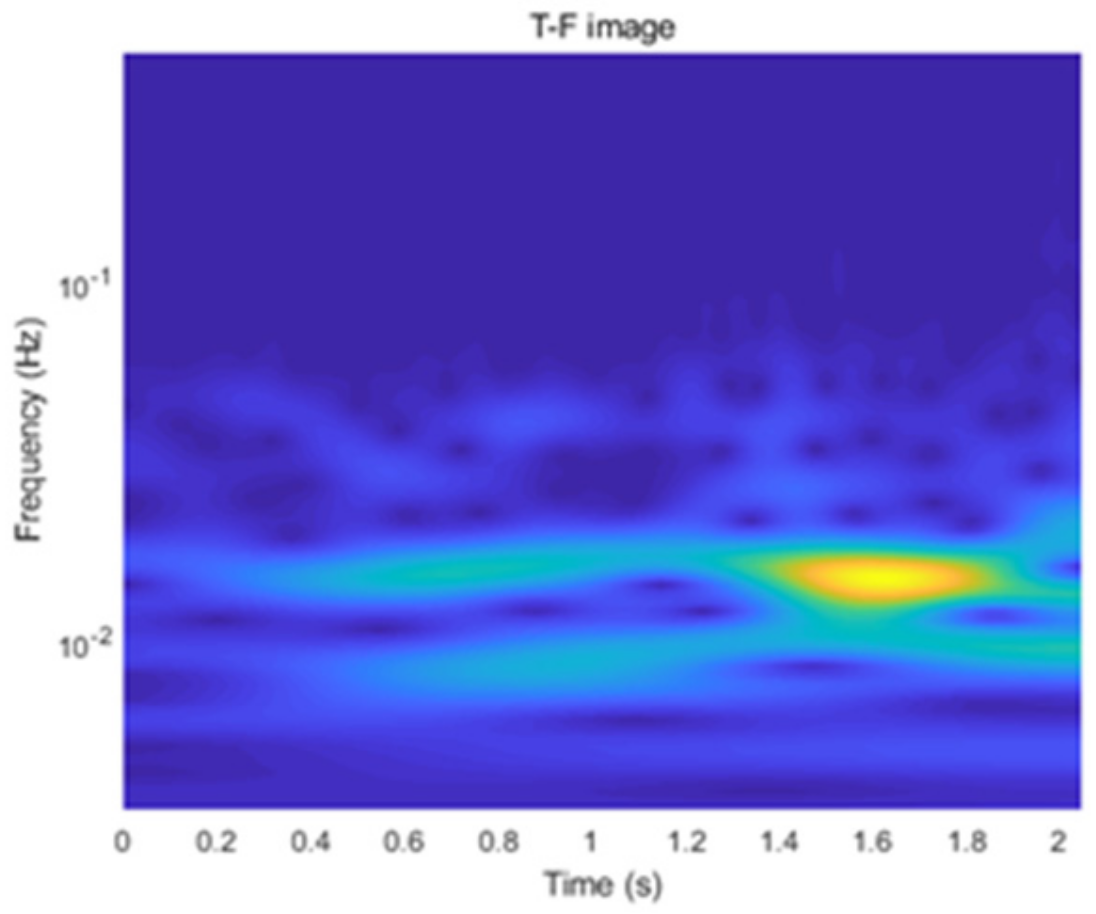
- The original acceleration signals are denoised using a median filtering method and are separated into segments. Then, the acceleration signal segments are processed through the Continuous Wavelet Transform (CWT) to generate Time-Frequency (T-F) images. These T-F images are stored as grayscale images and are labeled based on their dominant graphical features.
- The T-F images are used as input feature maps for CNNs to recognize the state of ASs.
- The final decision is obtained by fusing the preliminary recognition results using D-S evidence theory.
This paper describes this method in more detail, including the steps and methods used in each stage, in the rest of the paper.
2.1. Data Preprocessing
Measured acceleration signals typically include three types of noise: environmental noise, electrical noise, and mechanical noise. To extract the useful signal, the measured acceleration signals must be denoised in the data preprocessing stage. The authors use the median filtering method to reduce noise in this paper, and after denoising, the acceleration signals are separated into multiple segments for further processing.
The state recognition of ASs requires a feature vector that represents the acceleration signal segments. The success of the state recognition system depends on the features chosen to represent the acceleration signals in such a way that the differences among the acceleration waveforms are suppressed for waveforms of the same type, but emphasized for waveforms belonging to different types of states. In this paper, the authors propose using the CWT to perform the state recognition process of ASs on the acceleration signal segments, because the CWT can provide a useful representation or description of the signals.
The CWT of a signal f(x) in L2(R) space is defined as:
where <·> is an inner product operator; is the dilation of a basis wavelet φ(t) by the expansion scale factor α and the contraction scale factor τ. It is known that the CWT is well suited for analyzing non-stationary signals, and the Discrete Wavelet Transform (DWT) can perform an adaptive time-frequency decomposition of a signal. The multiresolution representation allows for describing the signal structure using only a few coefficients in the wavelet domain [35].
This paper describes the use of the wavelet toolbox function of Matlab to perform the CWT on the acceleration signals. The Morse wavelets are selected as the basis function for their good regularity and tight support. The acceleration signals are segmented and processed using the Morse (3, 60) wavelet, resulting in T-F images that are then compressed to a size of 100 × 100 and converted to grayscale images. This process is shown in Figure 2 and Figure 3.
2.2. CNN Decision
This section interprets the architecture of the designed CNNs models and introduces the functions of each layer in the CNN models. CNNs are a type of artificial neural network that are designed to process data with a grid-like topology, such as an image. They are inspired by the visual cortex of animals and have been widely used in tasks such as object detection and classification in images and videos [36].
A typical CNN architecture consists of several layers including an input layer, one or more convolutional layers, a max pooling layer, one or more fully connected layers, and a softmax output layer. The convolutional layers are responsible for identifying and extracting features from the input data, while the max pooling layers are used to reduce the spatial dimensions of the feature maps in order to increase the network’s ability to detect features at different scales. The fully connected layers are used to analyze the features and make a prediction, and the softmax output layer is used to produce a probability distribution over the possible classes of the input data.
2.2.1. Architecture of the CNN Models
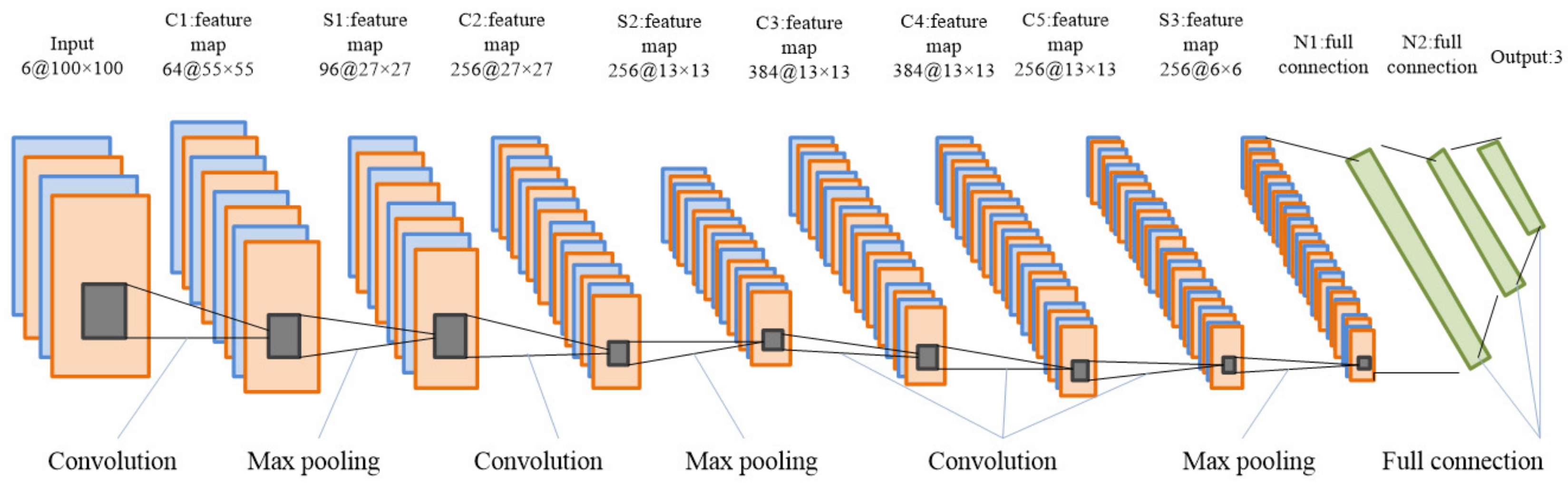
The architecture of the proposed CNN models is illustrated in Figure 4. The structure of the model is tailored to the specific task at hand, taking into account factors such as the number of sensors, data lengths, and number of prediction categories. This dictates the shape of the input and output layers. The main architecture of the inner layers is common to each CNN model.
The input to the network is a T-F grayscale image of size 100 × 100 × 6. The first layer is an input layer of the same size. The C1 convolutional layer applies 20 filters to the input image, generating 20 feature maps. Each filter produces a channel of the feature maps by sliding over the input image and computing a dot product between the filter and the local image patch. The resulting feature maps have a size of 55 × 55 × 20 (width, height, number of channels). The S1 max pooling layer performs max pooling with a pooling size of 3 × 3 and a stride size of 2 on each of the 20 feature maps generated by the previous layer. This downsamples each feature map by a factor of 2 along the width and height dimensions, resulting in 96 feature maps of size 27 × 27 × 20. The output of the S1 layer is flattened and fed into the N1 fully connected layer. This layer applies a linear transformation to the input followed by a nonlinear activation function (e.g., ReLU), producing a high-level representation of the input data. Finally, the output of the N1 layer is fed into the N2 softmax output layer, which produces a probability distribution over the possible classes of the input data. The predicted class is the one with the highest probability.
2.2.2. Illustration of CNNs
A CNN model has a special structural layer that is used to extract local features from the training data, which is called a convolutional layer. In this research, the input layer is convolved with learnable filters to form intermediate feature maps as follows:
where represents the jth channel of layer l; represents the ith channel of filter j in layer l; is a bias for filter j of layer l; I and J are the channel amounts of layer l-1 and l, respectively; f(·) denotes the activation function. Note that the feature maps acquired from the convolutional layer encode the local features, and their dimensions depend on those of the input data and convolutional kernels.
Pooling is a technique used in convolutional neural networks to reduce the spatial dimension of the feature maps, while retaining the most important information. This helps to reduce the computational complexity of the network and make it more robust to small changes in the input image. Common types of pooling include max pooling, which selects the maximum value from each pooling window, and average pooling, which computes the average value of the elements in each window.
After the inputs pass through the convolutional layers and max-pooling layers, a fixed-size feature representation is obtained. The next layers in the network are typically fully connected layers, which are used to transform the feature maps into a 1D layer and are fully connected to all the activations in the previous layer. The operations performed in the fully connected layer are represented by:
where is the jth neuron in full connection layer l, and J is the layer size. is a neuron in the previous 3D feature map l-1 (whether the feature map is the output of convolution or a pooling operation), with i1, i2, and i3 indicating positions in height, width, and channel, respectively. is the corresponding weight with between layer l-1 and layer l; is a bias in the input of ; f(·) denotes an activation function.
In the conventional CNN, the last layer is often a softmax layer, which is used to transform the output of the fully connected layer into a probability distribution, representing the likelihood of each class. The class with the highest probability is then selected as the output of the network.
2.3. Data Fusion
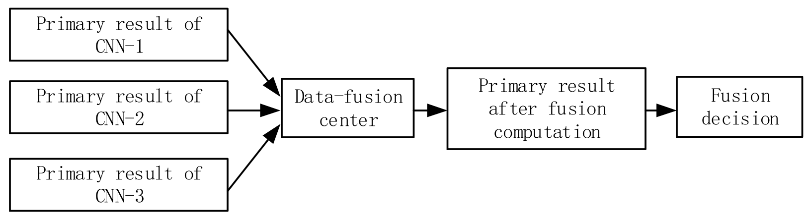
To improve the ability to process non-deterministic data and make use of large amounts of measurement data in recognizing the state of AS, three CNN models are constructed in Section 2.2. These models are used to obtain primary results, which are then input into a data fusion center. The flowchart in Figure 5 shows the data fusion process for state recognition. The key aspect of data fusion is the fusion algorithm, which can include methods such as the weighted average, Bayesian inference, and D-S evidence theory. In this specific paper, the authors use D-S evidence theory for the fusion computation [37].
D-S evidence theory is based on a finite and non-empty set called the frame of discernment, which contains n mutually exclusive and exhaustive hypotheses. The set is represented by:
where n is the number of hypotheses in the system, and Ai (i = 1, 2, …, n) represents the ith hypothesis that reflects the ith possible recognition result.
In order to describe the support degree for hypotheses, a basic probability assignment, also called the mass function, is introduced based on . The mass function is a function m: , which satisfies the following equations:
where m(A) is the basic support degree of evidence m to proposition A. If m(A) > 0, A is called the focal set.
Based on the mass function, the belief function (Bel) and plausibility function (Pl) on can be defined, respectively, as:
For ∀A ⊆ Θ, when two independent and reliable pieces of evidence m1 and m2 are separately obtained from two classifiers, the D-S combination rule can be defined as:
where K is the conflict factor that reflects the conflict degree of the two pieces of evidence m1 and m2, and it is given by:
Similarly, the combination rule of multiple evidence m1, m2, …, mn can be deduced as:
where K is given by:
In general, m(A) is the key element and difficulty, which directly affects the accuracy and effectiveness of the fusion decision result, but it is not given directly. Gray correlation analysis and fuzzy mathematics are employed to determine the correlation system and calculate the closeness [32]. This paper use closeness to construct and acquire the general form of m(A) [38], and the reasoning process of D-S evidence theory consists of three steps:
Step 1, calculation of closeness.
The closeness between the system’s frame (Θ) and the recognition result (outi) of each of the M classifiers is calculated using the formula:
where di,j is the distance between outi and Aj, and Di is the sum of distances.
Step 2, calculation of m(A).
mi(Aj) is given by:
Step 3, calculation of fusion results.
The fusion result is calculated by the basic mass function and the basic belief function using the Dempster synthesis rule. The maximum value satisfying the equation is:
where δ is a preset threshold. The output category is determined by this maximum value.
3. Experimental Verification
3.1. Example and Condition Description
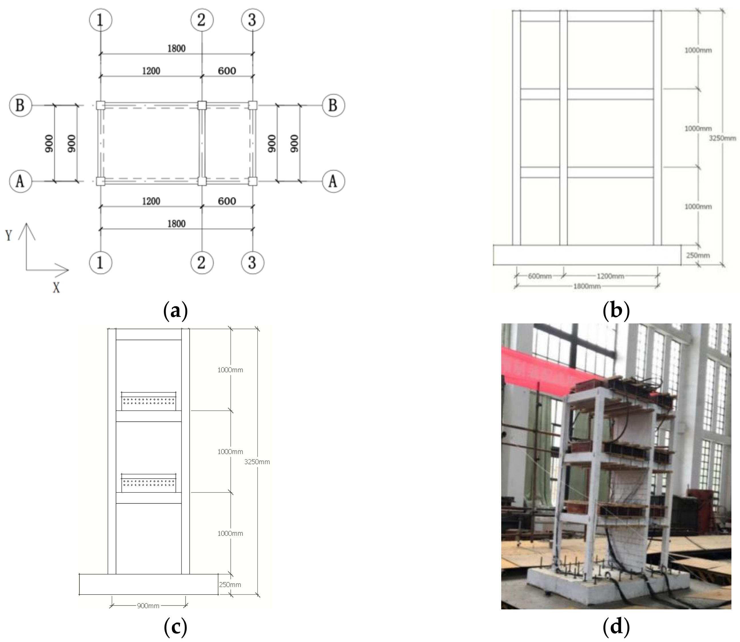
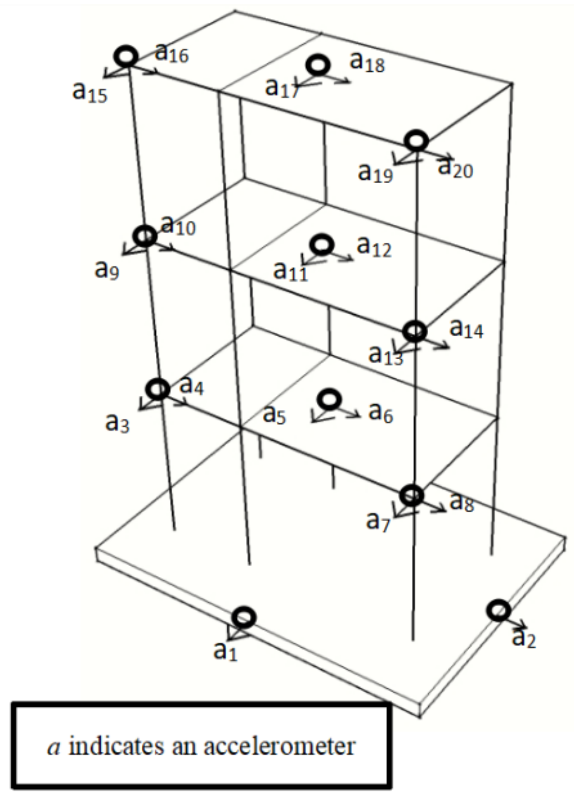
The proposed method was verified using shaking table vibration data from a three−story AS at Fuzhou University, as shown in Figure 6. The structure model was subjected to earthquakes with different wave patterns, including El−Centro, Taft, and Shanghai artificial (SHW2) waves [39,40]. The responses of the floors were recorded using 10 accelerometers, with 3 sensors assigned to each floor and 1 sensor assigned to the shaking table, as show in Figure 7. The recordings were made in both the south–north (X direction) and east–west (Y direction) of the structural model.
The AS was subjected to both random white noise for ambient vibration response recording and 9 levels of earthquake excitations with different intensities (0.1 g, 0.15 g, 0.2 g, 0.31 g, 0.4 g, 0.51 g, 0.62 g, 0.7 g, and 0.8 g). After each excitation, the structure model was visually monitored and classified into one of the three patterns: no damage, moderate damage, and large damage. The test schedule is summarized in Table 1.
3.2. Pattern Recognition of AS
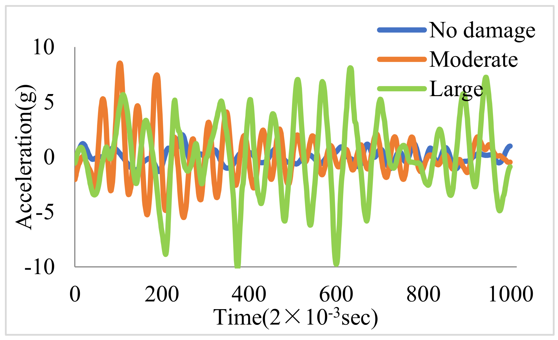
3.2.1. Signal Acquisition
The signal was acquired with a sampling frequency of 500 Hz. Figure 8 shows the time series signal of the AS under three different damage patterns. While there are differences in the signals for each damage pattern, it is not possible to directly identify the damage pattern from the time series signal alone.
3.2.2. Data Processing
The data processing was carried out using MATLAB. The collected acceleration signals were first denoised using the median filtering method and then divided into segments. Next, the acceleration signal segments were processed using the CWT to generate T-F images. The T-F images were then stored as grayscale images and labeled based on their dominant graphical features, as outlined in Section 2.1. For the purposes of this example, three signals from Figure 8 were selected and each T-F image was transformed into a grayscale image for simplicity. The T-F images were then compressed and resized to 100 × 100 for ease of analysis, as shown in Figure 9. In total, 807 sets of T-F images were generated, with 538 sets being used as the training set and the remaining 269 sets being used as the testing set.
3.2.3. Single CNN Model
In this study, a CNN model was constructed based on the specific parameters described in Section 2.2. The training samples were used to train the CNN model and the model was finalized when it fell within the specified tolerance or after reaching the specified number of iteration steps. The data from each floor were used as input for the single CNN model to create CNN-1, CNN-2, and CNN-3. The trained CNN model was then tested using the test samples, and the final decision results were obtained.
3.2.4. Data Fusion
The outputs from the three single CNN models were then fed into a data fusion center for combining. As described in Section 2.3, the D-S evidence theory was used to fuse the outputs from the three CNN models to make the final decision on damage detection.
3.3. Results and Discussion
3.3.1. Single CNN Decision Results
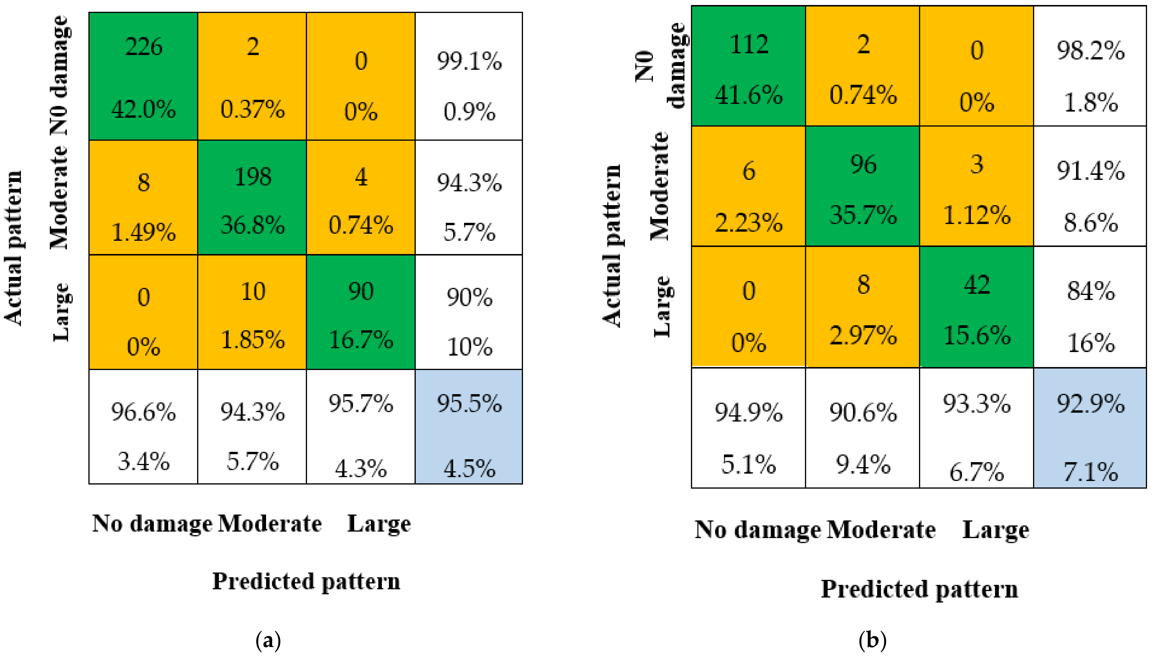
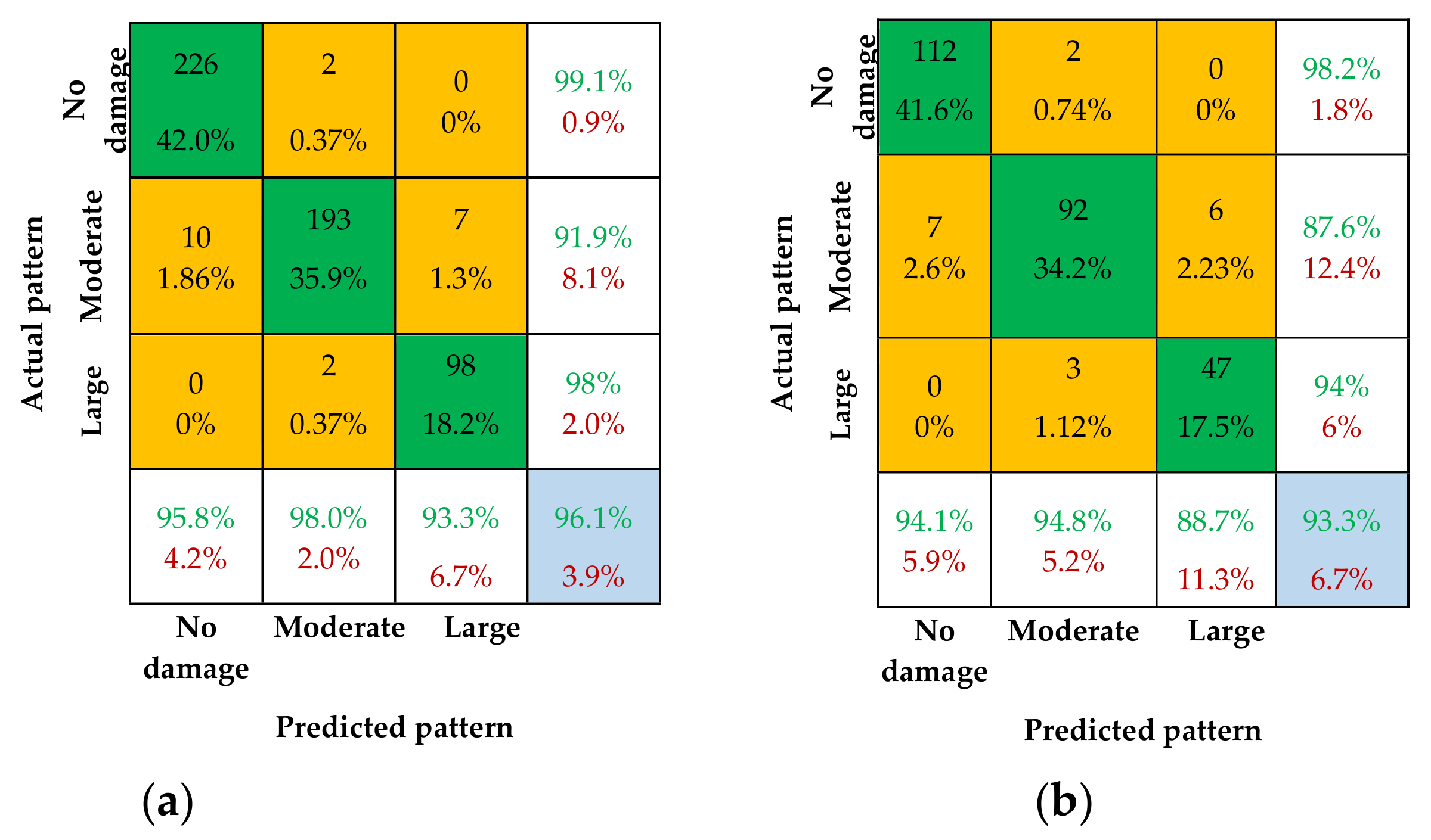
The results of the single CNN decision for the AS are presented in the form of confusion matrices in Figure 10, Figure 11 and Figure 12. The matrices show the predicted patterns (as predicted by the trained CNN) versus the actual patterns for the test cases. The diagonal cells indicate correctly identified patterns. Each cell shows the total number and percentage of predicted patterns compared to the total number of test/validation patterns. The off-diagonal cells represent misclassified test cases. The far-right column of the matrix displays the true and false prediction rates in percentage. The bottom row lists, for each pattern, the percentage of correctly and incorrectly predicted patterns. The overall identification accuracy (IA) of the test is indicated in the lower-right-hand corner cell of the matrix. It is important to note that the results are based on the respective training and test samples for each CNN model.
The results of this study show that among the three single CNN models, CNN-3 has the highest overall IA of 96.3% for training samples and 94.0% for test samples, as shown in Figure 12. CNN-2 has an overall IA of 96.1% for training samples and 93.3% for test samples, as shown in Figure 11, while CNN-1 has an overall IA of 95.5% for training samples and 92.9% for test samples, as shown in Figure 10. These results indicate that the single CNN model has a strong ability to recognize damage patterns.
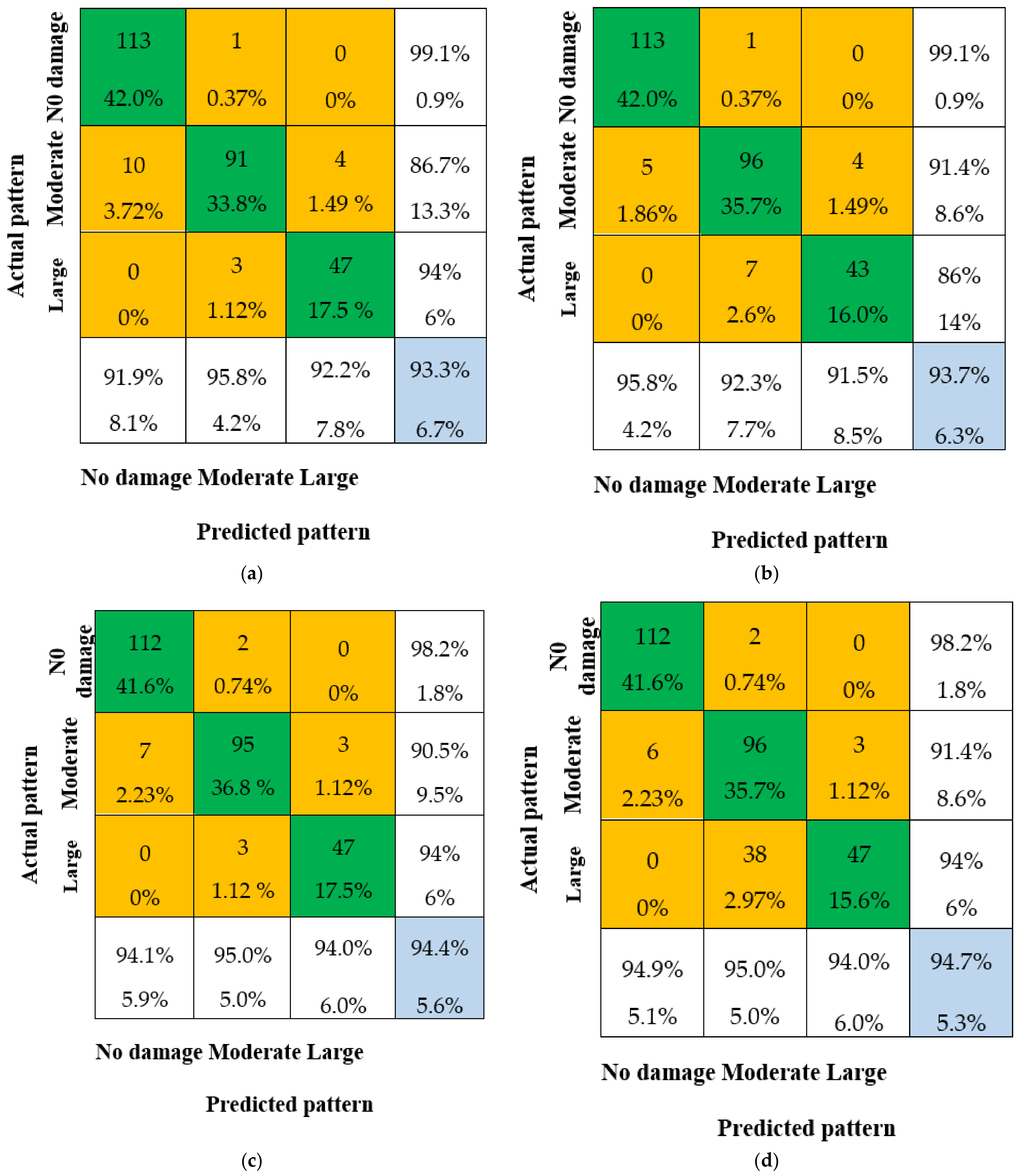
3.3.2. Fusion Decision Results
The overall IA of the fusion methods is shown in Figure 13 based on the results from Section 3.2.4. The following conclusions can be drawn from the findings:
- The pattern recognition ability of the fusion methods is significantly improved compared to the single CNN decision. The overall IA is not less than 93.3% for all four fusion methods, which is much better than the overall IA of CNN-1 (92.9%). This demonstrates that the data fusion method has a higher IA than any single CNN model.
- The overall IA for the combination of CNN-1 and CNN-2, and the combination of CNN-1 and CNN-3, is 93.3% and 93.7%, respectively, which is lower than the overall IA for the combination of CNN-2 and CNN-3. This is due to the lower overall IA of single CNN-1 compared to CNN-2 and CNN-3, which results in a lower overall IA after data fusion.
- The overall IA for the combination of all three CNN models (CNN-1 + CNN-2 + CNN-3) is 2%, 1.6%, and 0.8% higher compared to CNN-1, CNN-2, and CNN-3, respectively. This indicates that multi-sensor data fusion has a better pattern recognition capacity than any single CNN model.
4. Discussion
The method proposed in this paper has been tested with a small sample size due to the limited shaking table test data of ASs and the lack of actual engineering data. Therefore, the generalizability of our proposed method to other datasets may be limited. To validate the robustness and effectiveness of our approach, we plan to conduct further experiments on larger datasets in the future. Additionally, it should be noted that our method relies on preprocessing techniques such as denoising and the wavelet transform, which may not be applicable to all datasets or scenarios.
In the current experimental data, our proposed method has demonstrated a significantly improved recognition ability compared to the 1D CNN model in two aspects: recognition ability with different input images of the same patterns and recognition ability with similar T-F images from different patterns. Compare as follows:
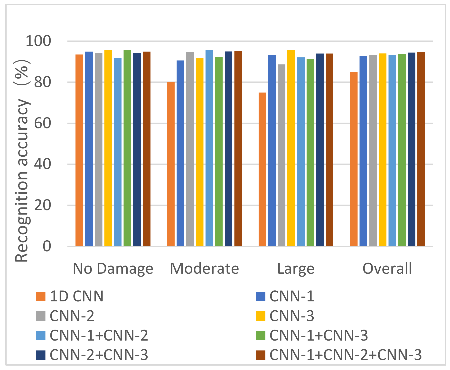
4.1. Comparison with Other Methods
For comparison purposes, a one-dimensional (1D) CNN model was also developed and tested. The 1D CNN model was designed to directly recognize the time series acceleration data, and its development process was similar to that of the AS state recognition model, except that the CWT was not included. The recognition results of the 1D and AS state recognition models are presented in Figure 14.
4.2. Recognition Ability with Different Input Images of the Same Patterns
The T-F images of the same patterns can be largely different when the structure is subjected to different earthquake excitations. Therefore, it is necessary to evaluate the ability of the CNN to identify the difference in the same patterns and to assess its generalization ability. As shown in Figure 15, the position and intensity of the T-F images are different for no damage under three earthquake excitations: El-Centro, Taft, and SHW2. The results show that the proposed method can identify the no-damage patterns with a recognition accuracy of 94.3%, 91.7%, and 92.5%, respectively. This indicates that the proposed method has good generalization abilities.
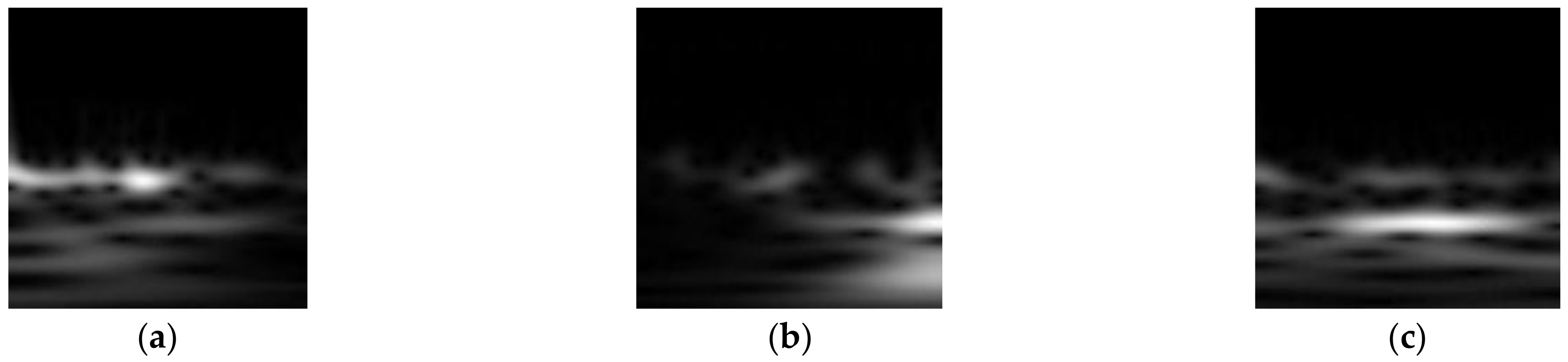
4.3. Recognition Ability with Similar T-F Images from Different Patterns
In order to evaluate the CNN’s ability to identify different patterns by using similar T-F images and assess its feature extraction capability, the T-F images were compared between no damage, moderate, and extensive patterns under SHW2 earthquake excitations, as shown in Figure 16. The results show that the proposed method can identify no damage, moderate, and extensive patterns with recognition accuracies of 92.5%, 90.4%, and 89.9%, respectively. This indicates that the proposed method has strong feature extraction capabilities.
5. Conclusions
This paper proposed a three−stage state recognition method for Assembled Structures (ASs) using Convolutional Neural Networks (CNNs) and data fusion. The method was evaluated on shaking table vibration data from a three-story AS subjected to different wave patterns and earthquake excitations. The experimental results demonstrate the effectiveness and generalization capability of the proposed method, with CNN-3 achieving the highest overall identification accuracy (IA) of 96.3% for training samples and 94.0% for test samples.
The proposed method has the potential to significantly improve the safety and maintenance of assembly structures by accurately identifying their state and facilitating informed decision−making. However, further research is required to fully validate its effectiveness under different conditions and in real-world scenarios. Future studies should focus on testing the method on various types of ASs under different environmental conditions, while also comparing its performance to other existing methods. By doing so, we can better understand the overall accuracy, reliability, and efficiency of the approach and its potential for practical implementation.
Author Contributions
Conceptualization, J.L. and S.J.; methodology, J.L.; software, J.L.; validation, J.L., J.Z. and Z.Z.; formal analysis, J.L.; investigation, J.L. and Z.Z.; resources, S.J.; data curation, Z.Z.; writing—original draft preparation, J.L.; writing—review and editing, J.L. and S.J.; visualization, J.L.; supervision, S.J.; project administration, S.J.; funding acquisition, S.J. All authors have read and agreed to the published version of the manuscript.
Funding
This research was funded by the National Natural Science Foundation of China (No. 52278295); the Scientific Research Fund of Institute of Engineering Mechanics, China Earthquake Administration (Grant No. 2020 EEEVL); the Guiding project for the industrial technology development and application of Fujian Province, China (Grant No. 2020Y0015).
Institutional Review Board Statement
Not applicable.
Informed Consent Statement
Not applicable.
Data Availability Statement
The data are available from the National Natural Science Foundation of China (No. 52278295); the Scientific Research Fund of Institute of Engineering Mechanics, China Earthquake Administration (Grant No. 2020 EEEVL); the Guiding project for the industrial technology development and application of Fujian Province, China (Grant No. 2020Y0015).
Acknowledgments
The authors would like to express their gratitude to the editors and reviewers for their constructive comments, which greatly improved the quality of this paper.
Conflicts of Interest
The authors declare no conflict of interest.
References
- Bo, Q. The ministry of housing and construction finalized eight key tasks in 2016. China Prospect Des. 2016, 1, 1–11. [Google Scholar]
- Ju, R.-S.; Lee, H.-J.; Chen, C.-C.; Tao, C.-C. Experimental study on separating reinforced concrete infill walls from steel moment frames. J. Constr. Steel Res. 2012, 71, 119–128. [Google Scholar] [CrossRef]
- Liu, X.; Bradford, M.A.; Lee, M.S.S. Behavior of High-Strength Friction-Grip Bolted Shear Connectors in Sustainable Composite Beams. J. Struct. Eng. 2015, 141, 04014149. [Google Scholar] [CrossRef]
- Ko, J.M.; Ni, Y.-Q.; Chan, H.-T.T. Dynamic monitoring of structural health in cable-supported bridges. Smart Struct. Mater. Smart Syst. Bridges Struct. Highw. 1999, 3671, 161–172. [Google Scholar] [CrossRef]
- Doebling, S.W.; Farrar, C.R. The State of the Art in Structural Identification of Constructed Facilities; Los Alamos National Laboratory: Santa Fe, NM, USA, 1999. [Google Scholar]
- Sohn, H.; Farrar, C.R.; Hemez, F.M.; Shunk, D.D.; Stinemates, D.W.; Nadler, B.R.; Czarnecki, J.J. A Review of Structural Health Monitoring Literature: 1996–2001; Los Alamos National Laboratory: Santa Fe, NM, USA, 2003; Volume 1, p. 16. [Google Scholar]
- Giordano, P.F.; Quqa, S.; Limongelli, M.P. The value of monitoring a structural health monitoring system. Struct. Saf. 2023, 100, 102280. [Google Scholar] [CrossRef]
- Avci, O.; Abdeljaber, O.; Kiranyaz, S.; Hussein, M.; Gabbouj, M.; Inman, D.J. A review of vibration-based damage detection in civil structures: From traditional methods to Machine Learning and Deep Learning applications. Mech. Syst. Signal Process. 2021, 147, 107077. [Google Scholar] [CrossRef]
- Homaei, F.; Shojaee, S.; Amiri, G. A direct damage detection method using ultiple damage localization index based on mode shapes criterion. Struct. Eng. Mech. 2014, 49, 183–202. [Google Scholar] [CrossRef]
- Abdeljaber, O.; Avci, O.; Kiranyaz, S.; Gabbouj, M.; Inman, D.J. Real-time vibration-based structural damage detection using one-dimensional convolutional neural networks. J. Sound Vib. 2017, 388, 154–170. [Google Scholar] [CrossRef]
- Hakim, S.J.S.; Irwan, M.J.; Ibrahim, M.H.W.; Ayop, S.S. Structural damage identification employing hybrid intelligence using artificial neural networks and vibration-based methods. J. Appl. Res. Technol. 2022, 20, 221–236. [Google Scholar] [CrossRef]
- Gomez-Cabrera, A.; Escamilla-Ambrosio, P.J. Review of Machine-Learning Techniques Applied to Structural Health Monitoring Systems for Building and Bridge Structures. Appl. Sci. 2022, 12, 10754. [Google Scholar] [CrossRef]
- Kiranyaz, S.; Waris, M.-A.; Ahmad, I.; Hamila, R.; Gabbouj, M. Face segmentation in thumbnail images by data-adaptive convolutional segmentation networks. In Proceedings of the 2016 IEEE International Conference on Image Processing (ICIP), Phoenix, AZ, USA, 25–28 September 2016; IEEE: New York, NY, USA, 2016; pp. 2306–2310. [Google Scholar]
- Hien, H.T.; Akira, M. Damage detection method using support vector machine and first three natural frequencies for shear structures. Open J. Civ. Eng. 2013, 3, 104–112. [Google Scholar]
- Lu, N.; Wu, Y.; Feng, L.; Song, J. Deep learning for fall detection: 3d-cnn combined with lstm on video kinematic data. IEEE J. Biomed. Health Inform. 2018, 23, 314–323. [Google Scholar] [CrossRef] [PubMed]
- Cho, K.; Van Merrienboer, B.; Bahdanau, D.; Bengio, Y. On the properties of neural machine translation: Encoder-decoder approaches. Comput. Sci. 2014, 1409, 1259. [Google Scholar]
- Ma, X.; Yang, H.; Chen, Q.; Huang, D.; Wang, Y. Depaudionet: An efficient deep model for audio based depression classification. In Proceedings of the 6th International Workshop on Audio/Visual Emotion Challenge, New York, NY, USA, 16 October 2016; pp. 35–42. [Google Scholar]
- Schlosser, J.; Chow, C.K.; Kira, Z. Fusing LIDAR and images for pedestrian detection using convolutional neural networks. In Proceedings of the 2016 IEEE International Conference on Robotics and Automation (ICRA), Stockholm, Sweden, 16–21 May 2016; pp. 2198–2205. [Google Scholar]
- Ebesu, T.; Yi, F. Neural citation network for context-aware citation recommendation. In Proceedings of the 40th International ACM SIGIR Conference on Research and Development in Information Retrieval, Tokyo, Japan, 7–11 August 2017; pp. 1093–1096. [Google Scholar]
- Tang, Z.; Chen, Z.; Bao, Y.; Li, H. Convolutional neural network-based data anomaly detection method using multiple information for structural health monitoring. Struct. Control. Health Monit. 2018, 26, e2296. [Google Scholar] [CrossRef]
- Arnab, A.; Zheng, S.; Jayasumana, S.; Romera-Paredes, B.; Larsson, M.; Kirillov, A.; Savchynskyy, B.; Rother, C.; Kahl, F.; Torr, P.H. Conditional Random Fields Meet Deep Neural Networks for Semantic Segmentation: Combining Probabilistic Graphical Models with Deep Learning for Structured Prediction. IEEE Signal Process. Mag. 2018, 35, 37–52. [Google Scholar] [CrossRef]
- Kerdvibulvech, C.; Saito, H. Vision-Based Detection of Guitar Players’ Fingertips Without Markers. In Proceedings of the Computer Graphics, Imaging and Visualisation (CGIV 2007), Bangkok, Thailand, 14–17 August 2007; pp. 419–428. [Google Scholar]
- Gers, F.A.; Schmidhuber, E. LSTM recurrent networks learn simple context-free and context-sensitive languages. IEEE Trans. Neural Netw. 2001, 12, 1333–1340. [Google Scholar] [CrossRef]
- Klapper-Rybicka, M.; Schraudolph, N.N.; Schmidhuber, J. Unsupervised learning in LSTM recurrent neural networks. In Proceedings of the Artificial Neural Networks—ICANN 2001: International Conference, Vienna, Austria, 21–25 August 2001; Volume 11, pp. 684–691. [Google Scholar]
- Zhang, Y.; Miyamori, Y.; Mikami, S.; Saito, T. Vibration-based structural state identification by a 1-dimensional convolutional neural network. Comput. Civ. Infrastruct. Eng. 2019, 34, 822–839. [Google Scholar] [CrossRef]
- Khodabandehlou, H.; Pekcan, G.; Fadali, M.S. Vibration-based structural condition assessment using convolution neural networks. Struct. Control. Health Monit. 2019, 26, e2308. [Google Scholar] [CrossRef]
- Xu, Y.; Wei, S.; Bao, Y.; Li, H. Automatic seismic damage identification of reinforced concrete columns from images by a region-based deep convolutional neural network. Struct. Control Health Monit. 2019, 26, e2313. [Google Scholar] [CrossRef]
- Tang, Y.; Huang, Z.; Chen, Z.; Chen, M.; Zhou, H.; Zhang, H.; Sun, J. Novel visual crack width measurement based on backbone double-scale features for improved detection automation. Eng. Struct. 2023, 274, 115158. [Google Scholar] [CrossRef]
- Broer, A.A.R.; Benedictus, R.; Zarouchas, D. The Need for Multi-Sensor Data Fusion in Structural Health Monitoring of Composite Aircraft Structures. Aerospace 2022, 9, 183. [Google Scholar] [CrossRef]
- Kashinath, S.A.; Mostafa, S.A.; Mustapha, A.; Mahdin, H.; Lim, D.; Mahmoud, M.A.; Mohammed, M.A.; Al-Rimy, B.A.S.; Fudzee, M.F.M.; Yang, T.J. Review of Data Fusion Methods for Real-Time and Multi-Sensor Traffic Flow Analysis. IEEE Access 2021, 9, 51258–51276. [Google Scholar] [CrossRef]
- Zhou, Q.; Zhou, H.; Zhou, Q.; Yang, F.; Luo, L.; Li, T. Structural damage detection based on posteriori probability support vector machine and Dempster–Shafer evidence theory. Appl. Soft Comput. 2015, 36, 368–374. [Google Scholar] [CrossRef]
- Jiang, S.-F.; Fu, D.-B.; Ma, S.-L.; Fang, S.-E.; Wu, Z.-Q. Structural Novelty Detection Based on Adaptive Consensus Data Fusion Algorithm and Wavelet Analysis. Adv. Struct. Eng. 2013, 16, 189–205. [Google Scholar] [CrossRef]
- Wu, R.-T.; Jahanshahi, M.R. Data fusion approaches for structural health monitoring and system identification: Past, present, and future. Struct. Health Monit. 2020, 19, 552–586. [Google Scholar] [CrossRef]
- Li, H.; Bao, Y.; Ou, J. Structural damage identification based on integration of information fusion and shannon entropy. Mech. Syst. Signal Process. 2008, 22, 1427–1440. [Google Scholar] [CrossRef]
- Zhao, Q.; Zhang, L. ECG Feature Extraction and Classification Using Wavelet Transform and Support Vector Machines. In Proceedings of the 2005 International Conference on Neural Networks and Brain, Beijing, China, 13–15 October 2005; Volume 2, pp. 1089–1092. [Google Scholar]
- Chan, T.-H.; Jia, K.; Gao, S.; Lu, J.; Zeng, Z.; Ma, Y. PCANet: A Simple Deep Learning Baseline for Image Classification? IEEE Trans. Image Process. 2015, 24, 5017–5032. [Google Scholar] [CrossRef]
- Ye, F.; Chen, J.; Li, Y. Improvement of DS Evidence Theory for Multi-Sensor Conflicting Information. Symmetry 2017, 9, 69. [Google Scholar] [CrossRef]
- Gros, X.E. Applications of NDT Data Fusion; Kluwer Academic Publishers: Boston, MA, USA, 2001; pp. 20–23. [Google Scholar]
- Rahman, M.A.; Sritharan, S. Seismic response of precast, posttensioned concrete jointed wall systems designed for low-to midrise buildings using the direct displacement-based approach. PCI J. 2015, 60, 38–56. [Google Scholar] [CrossRef]
- Liu, Z. Shaking Table Test Study on Cast-In-Situ RC Frame-Assembled Dry-Connected Shear Wall Structure; Fuzhou University: Fuzhou, China, 2018. (In Chinese) [Google Scholar]
Figure 1.
Schematic diagram of the proposed method.

Figure 2.
T-F image.

Figure 3.
T-F grayscale image.

Figure 4.
Architecture of the proposed CNN models.

Figure 5.
Data fusion for state recognition.

Figure 6.
The three-story AS in Fuzhou University. (a) Load direction; (b) Front elevation; (c) Front elevation; (d) Front elevation.
Figure 6.
The three-story AS in Fuzhou University. (a) Load direction; (b) Front elevation; (c) Front elevation; (d) Front elevation.

Figure 7.
The layout of acceleration sensors.

Figure 8.
The time series signal by a18 sensor.

Figure 9.
Compressed T-F image for different patterns. If there are multiple panels, they should be listed as: (a) No damage; (b) Moderate; (c) Large.
Figure 9.
Compressed T-F image for different patterns. If there are multiple panels, they should be listed as: (a) No damage; (b) Moderate; (c) Large.

Figure 10.
Confusion matrices with CNN-1. (a) Confusion matrix for training samples; (b) Confusion matrix test samples.
Figure 10.
Confusion matrices with CNN-1. (a) Confusion matrix for training samples; (b) Confusion matrix test samples.

Figure 11.
Confusion matrices with CNN-2. (a) Confusion matrix for training samples; (b) Confusion matrix test samples.
Figure 11.
Confusion matrices with CNN-2. (a) Confusion matrix for training samples; (b) Confusion matrix test samples.

Figure 12.
Confusion matrices with CNN-3. (a) Confusion matrix for training samples; (b) Confusion matrix test samples.
Figure 12.
Confusion matrices with CNN-3. (a) Confusion matrix for training samples; (b) Confusion matrix test samples.

Figure 13.
Confusion matrices for testing samples with different methods. (a) CNN-1 + CNN-2; (b) CNN-1 + CNN-3; (c) CNN-2 + CNN-3; (d) CNN-1 + CNN-2 + CNN-3.
Figure 13.
Confusion matrices for testing samples with different methods. (a) CNN-1 + CNN-2; (b) CNN-1 + CNN-3; (c) CNN-2 + CNN-3; (d) CNN-1 + CNN-2 + CNN-3.

Figure 14.
Identification accuracy for test samples with different methods.

Figure 15.
T-F images in no damage under different earthquake excitations. (a) El-Centro wave; (b) Taft wave; (c) SHW2 wave.
Figure 15.
T-F images in no damage under different earthquake excitations. (a) El-Centro wave; (b) Taft wave; (c) SHW2 wave.

Figure 16.
Different patterns in similar T-F images. (a) No damage; (b) Moderate; (c) Large.


Table 1.
Damage cases/patterns and description.
| ID | Description | Peak Table Acceleration (g) | Damage Pattern |
|---|---|---|---|
| A1-W | White noise | 0.05 g | No damage |
| A1 | El-Centro | 0.1 g | |
| A2 | Taft | 0.1 g | |
| A3 | SHW2 | 0.1 g | |
| B1-W | White noise | 0.05 g | |
| B1 | El-Centro | 0.15 g | |
| B2 | Taft | 0.15 g | |
| B3 | SHW2 | 0.15 g | |
| C1-W | White noise | 0.05 g | |
| C1 | El-Centro | 0.2 g | |
| C2 | Taft | 0.2 g | |
| C3 | SHW2 | 0.2 g | |
| D1-W | White noise | 0.05 g | Moderate damage |
| D1 | El-Centro | 0.31 g | |
| D2 | Taft | 0.31 g | |
| D3 | SHW2 | 0.31 g | |
| E1-W | White noise | 0.05 g | |
| E1 | El-Centro | 0.4 g | |
| E2 | Taft | 0.4 g | |
| E3 | SHW2 | 0.4 g | |
| F1-W | White noise | 0.05 g | |
| F1 | El-Centro | 0.51 g | |
| F2 | Taft | 0.51 g | |
| F3 | SHW2 | 0.51 g | |
| G1-W | White noise | 0.05 g | Large damage |
| G1 | El-Centro | 0.62 g | |
| G2 | Taft | 0.62 g | |
| H1-W | White noise | 0.05 g | |
| H1 | El-Centro | 0.7 g | |
| H2 | Taft | 0.7 g | |
| I1-W | White noise | 0.05 g | |
| I1 | El-Centro | 0.8 g |
Disclaimer/Publisher’s Note: The statements, opinions and data contained in all publications are solely those of the individual author(s) and contributor(s) and not of MDPI and/or the editor(s). MDPI and/or the editor(s) disclaim responsibility for any injury to people or property resulting from any ideas, methods, instructions or products referred to in the content. |
© 2023 by the authors. Licensee MDPI, Basel, Switzerland. This article is an open access article distributed under the terms and conditions of the Creative Commons Attribution (CC BY) license (https://creativecommons.org/licenses/by/4.0/).
Share and Cite
MDPI and ACS Style
Luo, J.; Jiang, S.; Zhao, J.; Zhang, Z. An Integrated Method Based on Convolutional Neural Networks and Data Fusion for Assembled Structure State Recognition. Sustainability 2023, 15, 6094. https://doi.org/10.3390/su15076094
AMA Style
Luo J, Jiang S, Zhao J, Zhang Z. An Integrated Method Based on Convolutional Neural Networks and Data Fusion for Assembled Structure State Recognition. Sustainability. 2023; 15(7):6094. https://doi.org/10.3390/su15076094
Chicago/Turabian StyleLuo, Jianbin, Shaofei Jiang, Jian Zhao, and Zhangrong Zhang. 2023. "An Integrated Method Based on Convolutional Neural Networks and Data Fusion for Assembled Structure State Recognition" Sustainability 15, no. 7: 6094. https://doi.org/10.3390/su15076094
Note that from the first issue of 2016, this journal uses article numbers instead of page numbers. See further details here.