An Evaluation of the Dynamics of Some Meteorological and Hydrological Processes along the Lower Danube

Abstract

The objective of the present work was to perform a 30-year analysis of some significant meteorological and hydrological processes along the Lower Danube. This was motivated by the fact that, due to the effects of climate change, the global configuration of the environmental matrix has suffered visible transformations in many places. Another important factor considered is related to the constant development noticed in the last few decades of European inland navigation, in general, and in the Lower Danube sector, in particular. From this perspective, the processes analysed were the wind speed at a 10 m height, the air temperature at a 2 m height, precipitation, and river discharge. The 30-year period of 1991–2020 was considered for analysis. The ERA5 reanalysis data were processed and analysed in the case of the first three processes, while for the river discharge, the data provided by the European Flood Awareness System were used. The emphasis was placed on the evolution of the extreme values and on the identification of the geographical locations with a higher probability of occurrence. The average values and the seasonal variations of the four processes were also considered. The results indicated that the maximum wind speed and air temperature values along the Lower Danube did not suffer significant changes in the last few decades. However, the values of the minimum air temperatures increased with an average value of about 0.8 °C per decade, and the same tendency was noticed also for the average temperatures. Regarding the precipitation, the trend indicated a tendency to decrease by about 0.5 mm per decade, while for the river discharge, a clear increase of more than 1200 m³/s corresponded to each ten-year period. Finally, it can be concluded that the present analysis provided a global and more comprehensive perspective of the recent environmental dynamics along the Lower Danube, delivering useful information for inland navigation, as well as for other human activities.

1. Introduction

The Danube River originates from the Black Forest Mountains in Germany and flows in the southeastern direction for more than 2800 km, passing through, or bordering, ten European countries (Germany, Austria, Slovakia, Hungary, Croatia, Serbia, Romania, Bulgaria, Moldavia, and Ukraine) [1]. Regarding its length, the Danube is the second-longest European river after the Volga, in Russia. The Danube’s basin can be sectioned into three main parts, separated by “gates”, where the river is forced to pass the mountains [2]. These are: the Upper Danube, extending from the spring to the Devin Gate (at the border between Austria and Slovakia), the Middle Danube (also known as the Pannonia or Carpathian Basin), extending between the Devin Gate and the Iron Gates (at the border between Serbia and Romania), and the Lower Danube, extending from the Iron Gates to the river mouths at the Black Sea. The Danube represents the most-significant water resource of the Black Sea [3], and at its mouths, strong interactions between waves and the currents generated by the river outflow occur, together with some other significant coastal processes [4]. The Danube Delta is the largest and best-preserved delta of the European continent [5]. In the deltaic zone, the river outflow is through three principal branches, the Chilia, Sulina, and Saint George [6], and it is often subjected to floods and/or other hazards [7].

The Danube’s bottom gradients vary from 0.0012% (12 ppm) in the Upper Danube from the spring until the German city of Passau, and the gradient decreases to about 0.0006% (6 ppm) for the rest of the sector. Along the Middle Danube, the river becomes wider and the gradient becomes only 0.00006% (0.6 ppm), while in the Lower Danube, the mean value of the gradient is the lowest, being around 0.00003% (0.3 ppm) [8].

Many tributaries of the Danube River (more than 60) can be counted from the source to the river outflow in the Black Sea [9], among which, 32 are more significant and the Tisza River the longest. Many of them are also important navigable rivers [10]. The Maritime Danube extends from the Sulina at the Black Sea (RKM 0) and up to the port of Braila (RKM 170), and the river is navigable also by ocean ships, while river ships can navigate upstream to Ulm, in Germany [11]. Since 1992, when the Rhine–Main–Danube canal was inaugurated, the Danube River became part of the most-important inland navigation system in Europe. This is the seventh Pan-European transport corridor linking the Black and North Seas via a 3500 km-long waterway. This allows the navigation of large-scale river vessels, but larger ships can also navigate many parts of this system.

Besides navigation, the Danube represents also a viable source of renewable energy. With a total of 59 dams built along the first 1000 kilometres of the Danube down from its spring, the Upper Danube is considered very appropriate for hydropower plants, especially due to the natural gradient of the river in this region [12,13]. On the other hand, the Iron Gates Dams I and II in the Lower Danube sector represent the largest hydropower system along the river. This is composed of two dams, operated in common by Romania and Serbia and providing about 27% of the total energy used in Romania and 37% of the total energy demand of Serbia [14]. Moreover, taking into account the visible effects of climate change and the measures considered in the direction of decarbonisation [15], there is a significant and increasing interest in developing hydropower plants [16]. However, such constructions can cause various river and habitat interruptions and can also generate relevant changes in the natural structure of the river [17], producing pollution [18,19] and increasing the level of heavy metals in the water [20], and may also have a negative impact on fish diversity [21].

In this context, the objective of the present work was to perform an analysis related to the recent dynamics of the environmental matrix along the Lower Danube. Such an analysis allowed a better perspective concerning the evolution in the last 30 years of some significant meteorological or hydrological processes such as the variations of the wind speed, air temperature, precipitation, or river discharge. The emphasis was placed on the occurrence of the extreme values that have been noticed in the Lower Danube sector according to the data analysed, as well as on the identification of the geographical locations where such events are more probable. Several previous studies, for example [22], indicated that, due to climate changes, an enhancement of the frequency and especially of the intensity and duration of extreme events can be noticed along the Danube River. Furthermore, the present study aimed to identify also the last years’ dynamics of the extreme events and eventually to notice the possible future trends. Together with the analysis of the maximum values, the average values of the environmental processes, as well as their seasonal variations were also analysed and discussed.

Since the main target of the present work was to support inland navigation and harbour operations, it has to be highlighted that the processes analysed (wind speed, air temperature, precipitation, and river discharge) are extremely significant from this perspective. At the same time, it can be underlined at this point that the main novelty and added value of the present work are that 30 years of environmental data were processed and analysed along the entire Lower Danube, identifying also the sectors where there is a higher probability of extreme values in the environmental matrix, which can produce significant difficulties for inland navigation.

Finally, the gaps in some recent studies also have to be highlighted, for example [23,24], which the present work intended to fill through the results presented. This is to provide a global and more comprehensive perspective of the Lower Danube concerning the evolution over the last three decades of some meteorological and hydrological processes, especially focused on the extreme values of the relevant processes analysed, data that are significant not only for inland navigation, but also for many other human activities taking place along the river.

2. Materials and Methods

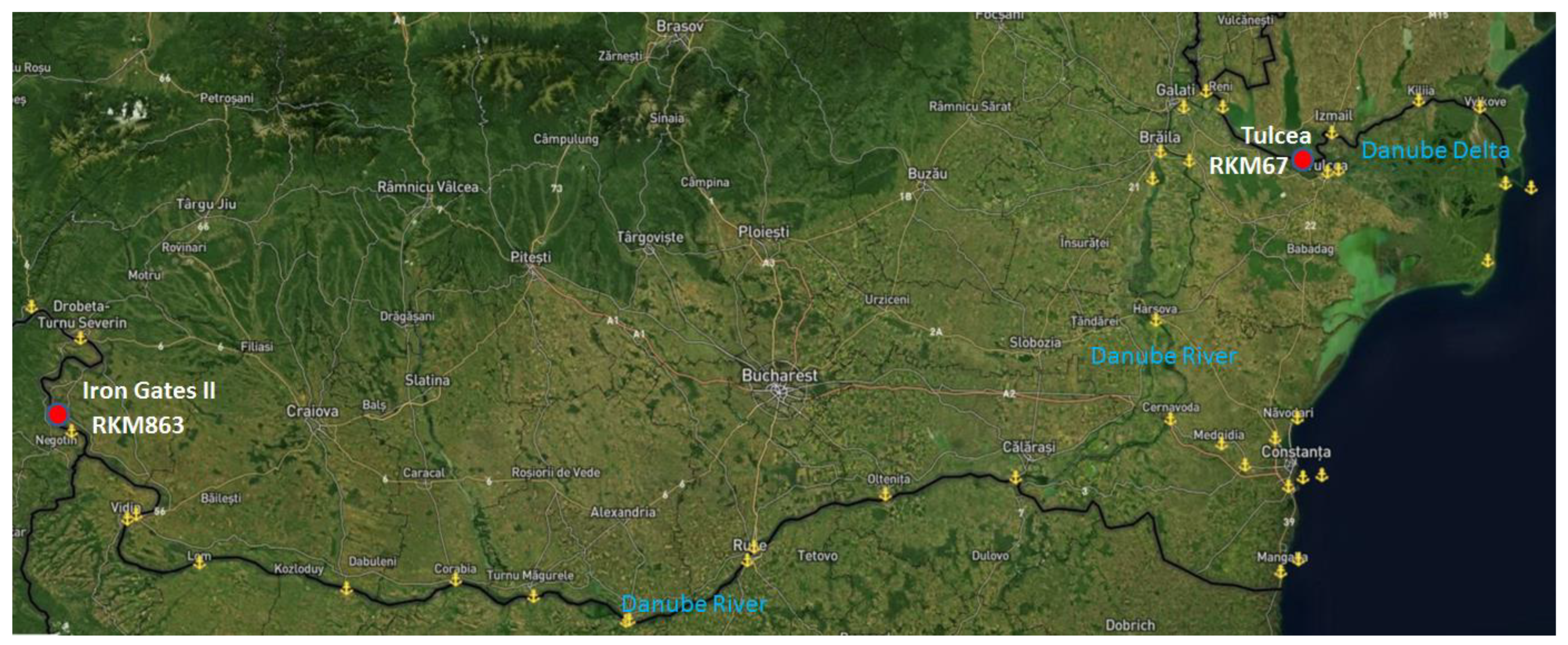
2.1. Target Area

The target area of the present study was the Lower Danube, more precisely the river sector located between Iron Gate II (RKM 863) and the city of Tulcea (RKM67) (Figure 1). Since the Danube Delta is a very special and complex area, the above-mentioned sector represents in fact the entire Lower Danube. This sector has a very dynamic riverbed with large flow rates (between <1600 m³/s and >15,000 m³/s). Its geography is very diverse. It includes mountains, large plains, sand dunes, and forested or marshy wetlands. Similarly, the climate and precipitation vary significantly; they continuously form the basin’s landscapes. The morphological processes in the Lower Danube are also quite dynamic. In the upper part of the section (km 863—km 730), the intensity of erosion and accumulation is less than in the middle (km 730—km 500) or in the lower part of the section (km 500–km 67). Consequently, hundreds of kilometres at both the left and right sides of the Danube River are strongly eroded.

In the last few decades, almost 75% of the floodplains of the Lower Danube were cut off from the main river by dikes and were transformed into agricultural areas, inducing impacts also on the flooding regimes. Furthermore, as highlighted before, riverbed erosion became a common phenomenon for large parts of this sector of the Danube. The conversion of plain forest to agriculture represents another important factor in enhancing extreme flood events. Such recent flood events in the Lower Danube River were noted especially in the years 2002, 2005, 2006, 2009, 2010, 2013, and 2014. On the other hand, the very low water levels reached in the Lower Danube sector in the last few years are damaging both the environment and the economy. Such a significant lowering of the water level also induces complex changes of the neighbouring river territories. Navigation represents another important issue in the Lower Danube sector, and as can be noticed in Figure 1, many ports are located along this Danube sector or in its vicinity. Four relevant factors are driving the dynamics of the Lower Danube sector. These are: agriculture, flood protection, transport, and climate change. Climate change is expected to further increase the flood risk along the entire Lower Danube sector, in terms of the intensity, duration, and frequency of the events. There is also a higher possibility of flash flood events during dry periods. However, there is also considerable uncertainty in the quantification of the future flood events due to the many shortcomings that may occur in the estimation of the future precipitation. Climate change is increasingly causing stressors, either hydrological, chemical, and/or thermal. As a consequence, the Lower Danube River sector can suffer from low water levels, especially at the end of the summer and at the beginning of the autumn seasons, with significant impacts both on the ecosystem and human activities. According to some recent studies [26], the air temperature is expected to increase with a gradient from northwest to southeast. Thus, from 2021 to 2050, an annual increase of 4 °C in the basin of the Lower Danube is expected, while between 2071 and 2100, an increase of about 5 °C is expected. As a consequence, at the end of the 21st Century, the air temperature increase is expected to be particularly great during summer, especially in the southeastern region of the Lower Danube.

2.2. Datasets Considered

The reanalysis data were provided by the ERA5 project, and they are made available to the public domain via the Copernicus Climate Change Service [27]. These data are based on the previous ERA-Interim and ERA-40 datasets and combine numerical simulations with various in situ observations. The accuracy of this dataset has been analysed in various riverine and coastal areas, and it has been found to be quite reliable [28]. A 30-year time interval (from January 1991 to December 2020) was considered for the evaluation. The dataset includes hourly values (24 per day) for each type of parameter. As mentioned in the ERA5 documentation [27], the environmental processes provided are averaged over a rectangular grid, and for this reason, some differences may be noticed if comparing to the direct measurements coming from a particular in situ station. The ERA5 reanalysis data processed and analysed in the present work are the wind speed at a 10 m height (U₁₀), the air temperature at a 2 m height (T₂), and precipitation. The third meteorological process (precipitation) represents the accumulated precipitation that falls to the Earth’s surface, which is generated by the convection scheme in the ECMWF Integrated Forecasting System (IFS), and it includes both rain and snow. This is accumulated over a particular time period, which depends on the data extracted. For the reanalysis, the accumulation period is over 1 h, ending at the validity date and time. The units corresponding to this process are depth in meters of water equivalent. This represents the depth the water would have if it were spread evenly over the grid box. At this point, it has to be highlighted that, for all three processes with the data coming from ERA5, the time step considered for the data was 3 h.

The last process analysed is the river discharge, as provided by the historical data from the European Flood Awareness System [29]. The river discharge (RD) in the last 24 h was considered for analysis in this work. This represents the volume rate of water flow (in m³/s), including sediments, chemical, and biological material, in the river channel averaged over a time step through a cross-section. The value is an average over each 24 h time step.

The data corresponding to all processes analysed were interpolated from the grid to the main navigation course of the Lower Danube without taking into account various secondary branches that occur along this sector of the Danube.

Some additional explanations concerning the statistical parameters evaluated and analysed will be provided at this point. Thus, for the 30-year time interval considered (1991–2020), the time series corresponding to data associated with the three meteorological processes (wind speed, temperature, and precipitation) with a 3 h time step and with a 24 h time step for the river discharge were analysed.

The first step is represented by the extreme value analysis, when the maximum values were evaluated together with the 99th and 95th percentiles. As is well known, the maximum is the highest value of a time series. On the other hand, the percentiles allow for the analysis of the data in terms of percentages and provide an image of the extreme values encountered in the areas studied. As an example, the 95th percentile indicates the value below which 95% of the data are found and above which only 5%. The 50th percentile represents the median of the distribution (or second quartile (Q2)), while the 75th percentile is the third quartile (Q3). In the cases of the temperature and river discharge, where the minimum values are also relevant, together with the maximum values, the 99th and 95th percentiles, also the minimum values, the 1st and 5th percentiles were also evaluated.

Another statistical analysis is related to the evaluation of the linear trend of the maximum and minimum annual series. A trend line, which is also called the line of best fit, is described by a linear relation as follows:

y = sx + m,

(1)

where x is the independent variable, y is the dependent variable, s is the slope of the line, and m is the y intercept. The regression parameters (s and m) were estimated by using the ordinary least-squares (OLS) method. The OLS estimators are obtained with the following relations:

$$s=\frac{{\sum }_{i=n}^n\left(x_i-\overline{x}\right)\left(y_i-\overline{y}\right)}{{\sum }_{i=1}^n{\left(x_i-\overline{x}\right)}^2}$$

(2)

$$m=\overline{y}-s\overline{x}$$

(3)

where n is the number of years for which the maximum (or minimum) annual values were calculated (in this case, 30 years), x is the independent variable represented by each year, and y is the dependent variable represented by the maximum value corresponding to each year. A five-year running average (or moving average) was also applied to the annual maximum and minimum series to filter the data variability, using the Matlab function dedicated to calculating the simple moving average of a vector. This is a technique to obtain an overall idea of the trends in a dataset, and it is an average of any subset of numbers, in this case being five values. Five indicates the number of previous data points used with the current data point when calculating the moving average.

As a second step, the mean values were also evaluated and analysed. These were computed using the standard definition of the mean:

$$\overline{X}=\mu =\frac{{\sum }_{i=1}^N{X}_i}{N}$$

(4)

where X_i represents the value of i from the time series and N is the number of data in the series.

3. Results

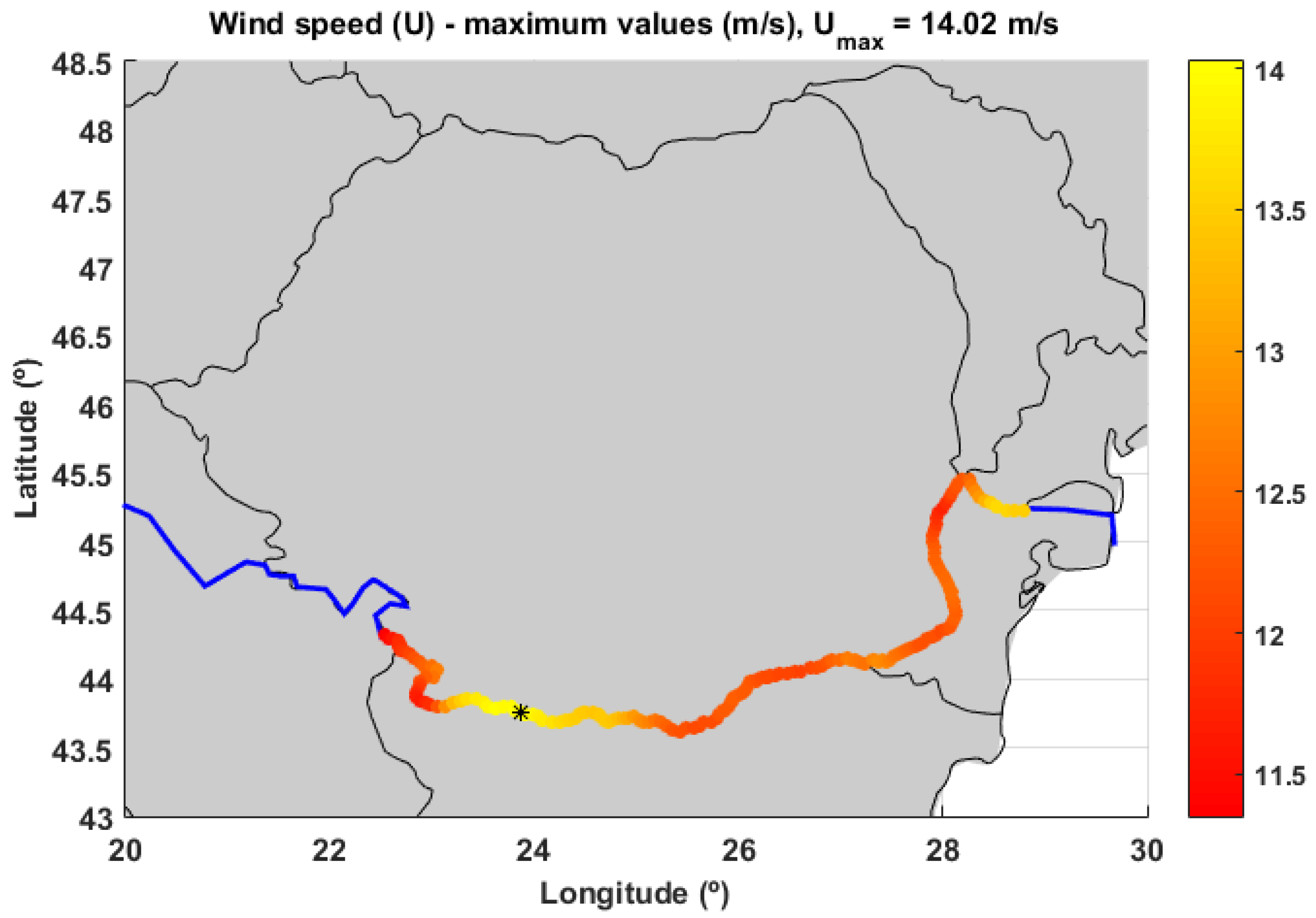
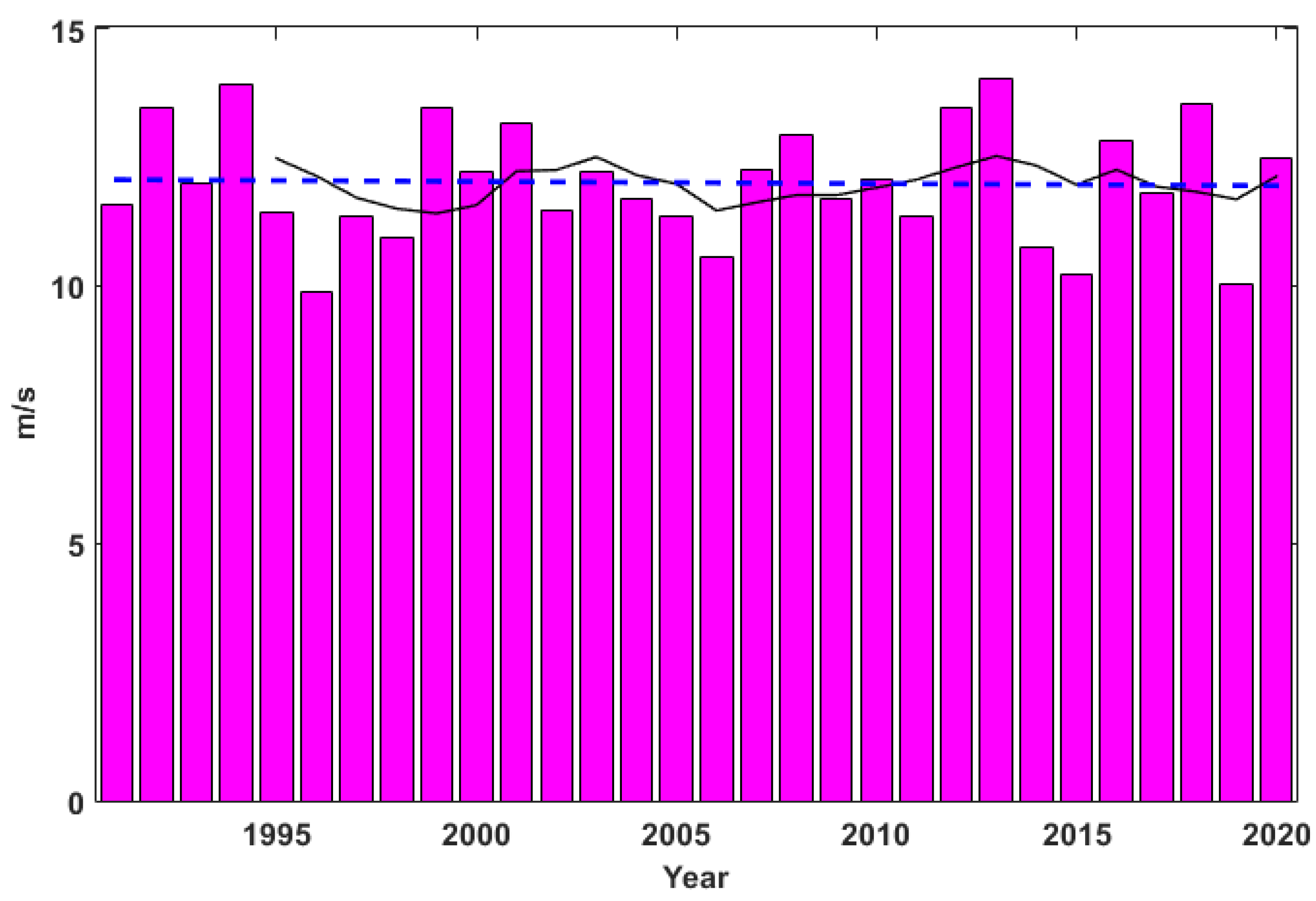
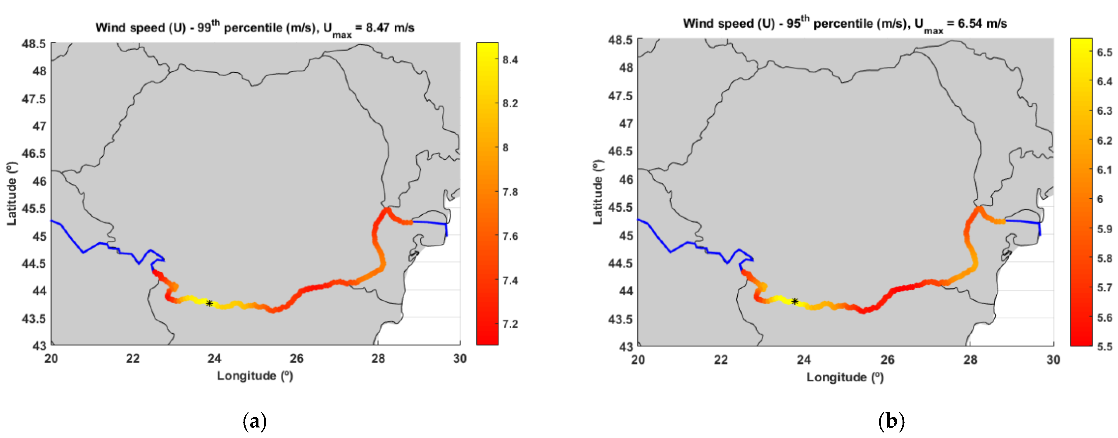
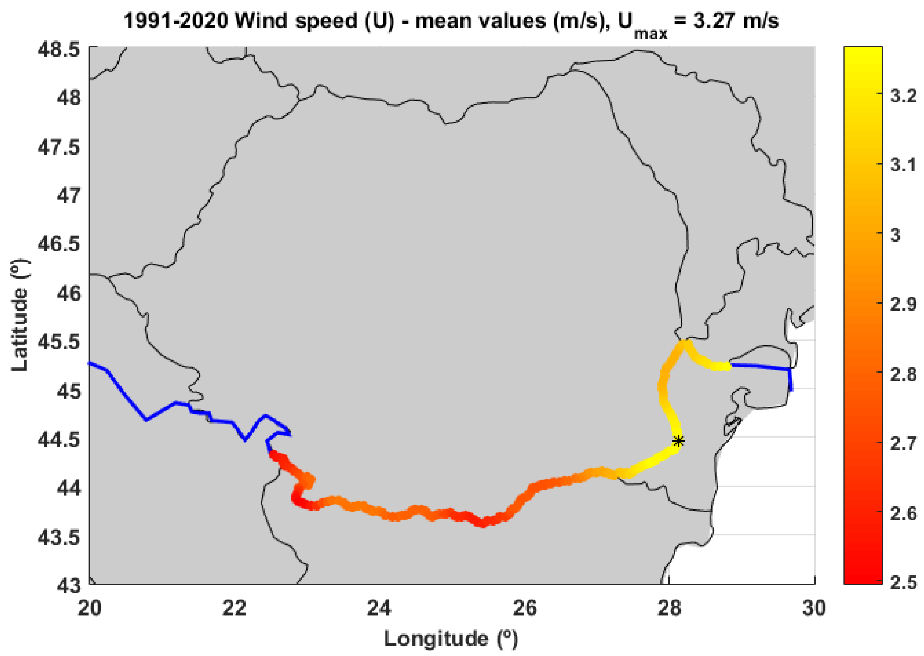
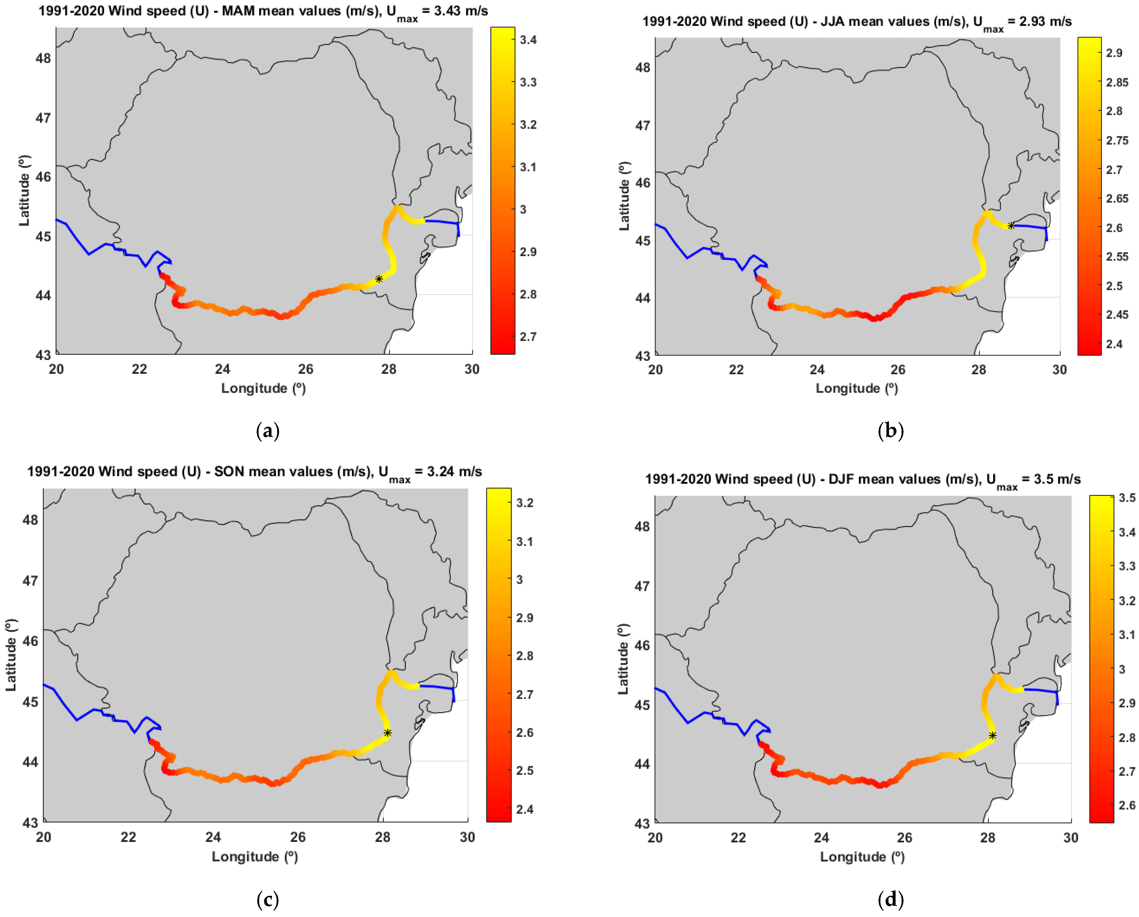
3.1. Wind Speed Analysis

The first analysis carried out was related to the wind speed at a 10 m height (U₁₀). Figure 2 illustrates the distribution of the maximum wind speed values (U_10max) along the Lower Danube for the 30-year time interval of 1991–2020. As can be noticed from this figure, the maximum value (around 14 m/s) occurred in the superior part of the sector, close to the Bulgarian city of Kosloduy (a place where a nuclear power plant is operational). Further on, Figure 3 presents the U₁₀ annual maximum series (bars) corresponding to the 30-year time interval considered. In this figure, the linear regression (indicating the trend) and the moving averages are also illustrated. The slope of the linear regression indicates the tendency of a very small increase for the maximum wind speed, with about 0.04 m/s in 10 years. If we compare the results with the neighbouring coastal environment at the Black Sea [28], it can be noticed that the maximum wind speeds are considerably higher (with about 10 m/s) in the nearshore of the Black Sea than along the Lower Danube. Furthermore, in the marine area, the trend indicates a more accentuated tendency of wind speed enhancement. The 99th and 95th percentiles of the wind speed along the Lower Danube for the same 30-year time interval analysed are presented in Figure 4. The results indicate that less than 1% of the wind speeds are higher than 8.5 m/s, while more than 95% of the wind speeds are lower than 6.5 m/s. In both cases, the geographical position of the maximum remains in the same location as that illustrated in Figure 2. Figure 5 presents the average wind speed values along the Lower Danube for the 30-year time interval of 1991–2020, where it can be noticed that these average values are between 2.5 and 3.3 m/s. Finally, the seasonal distributions of the average wind speeds along the Lower Danube for the time interval considered are illustrated in Figure 6. As expected, the higher wind speeds are in winter (with average values between 2.6 and 3.5 m/s) and the lower in summer (with average values between 2.4 and 2.9 m/s). Spring and autumn seasons present very similar characteristics, spring having slightly higher wind speed values (with averages between 2.7 and 3.4 m/s) than autumn (with averages between 2.4 and 3.2 m/s). Except for the summer, when the geographical location of the maximum is at the limit of the sector considered (close to the Romanian city of Tulcea), in all other seasons, the location of the maximum average wind speed value is close to the Romanian city of Cernavoda (where a nuclear power plant is operational).

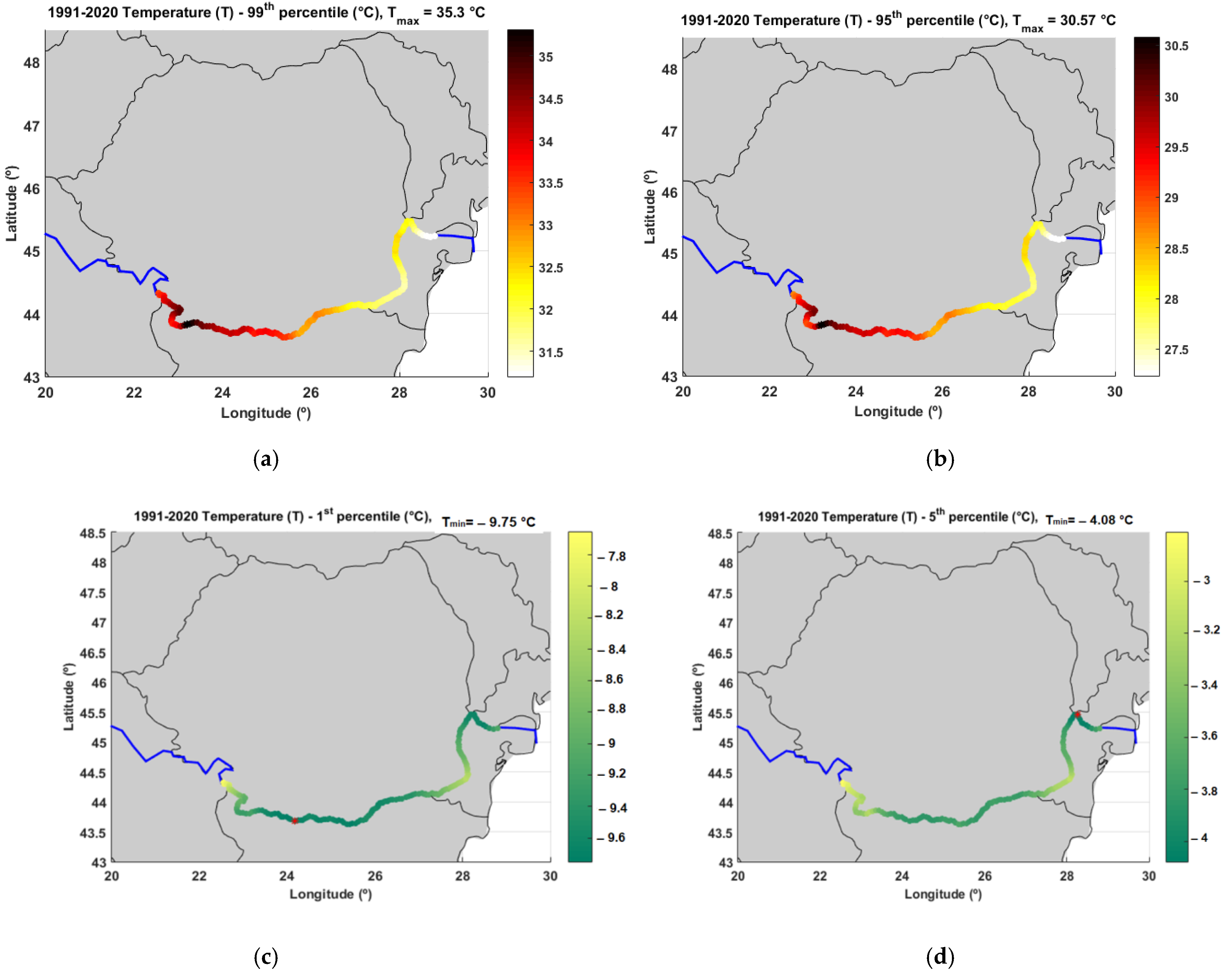
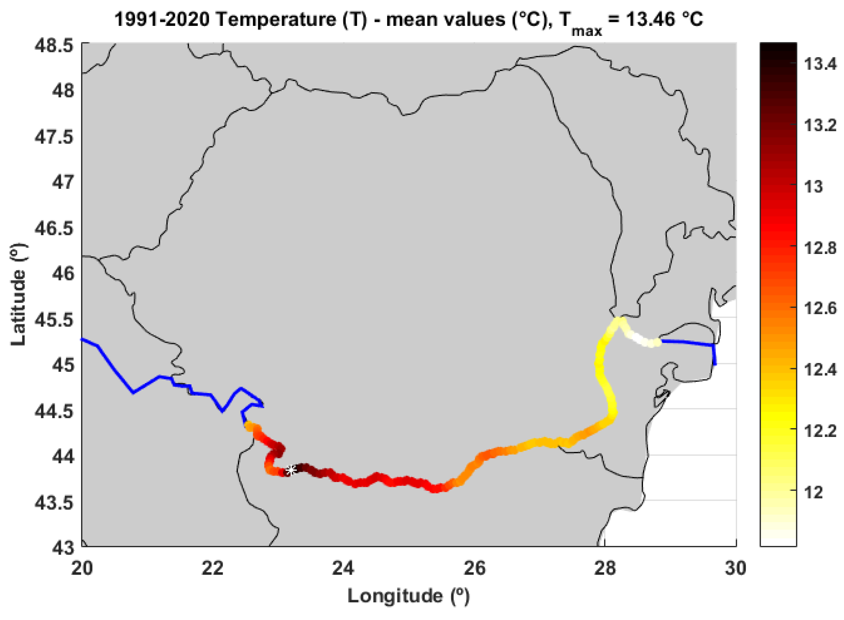
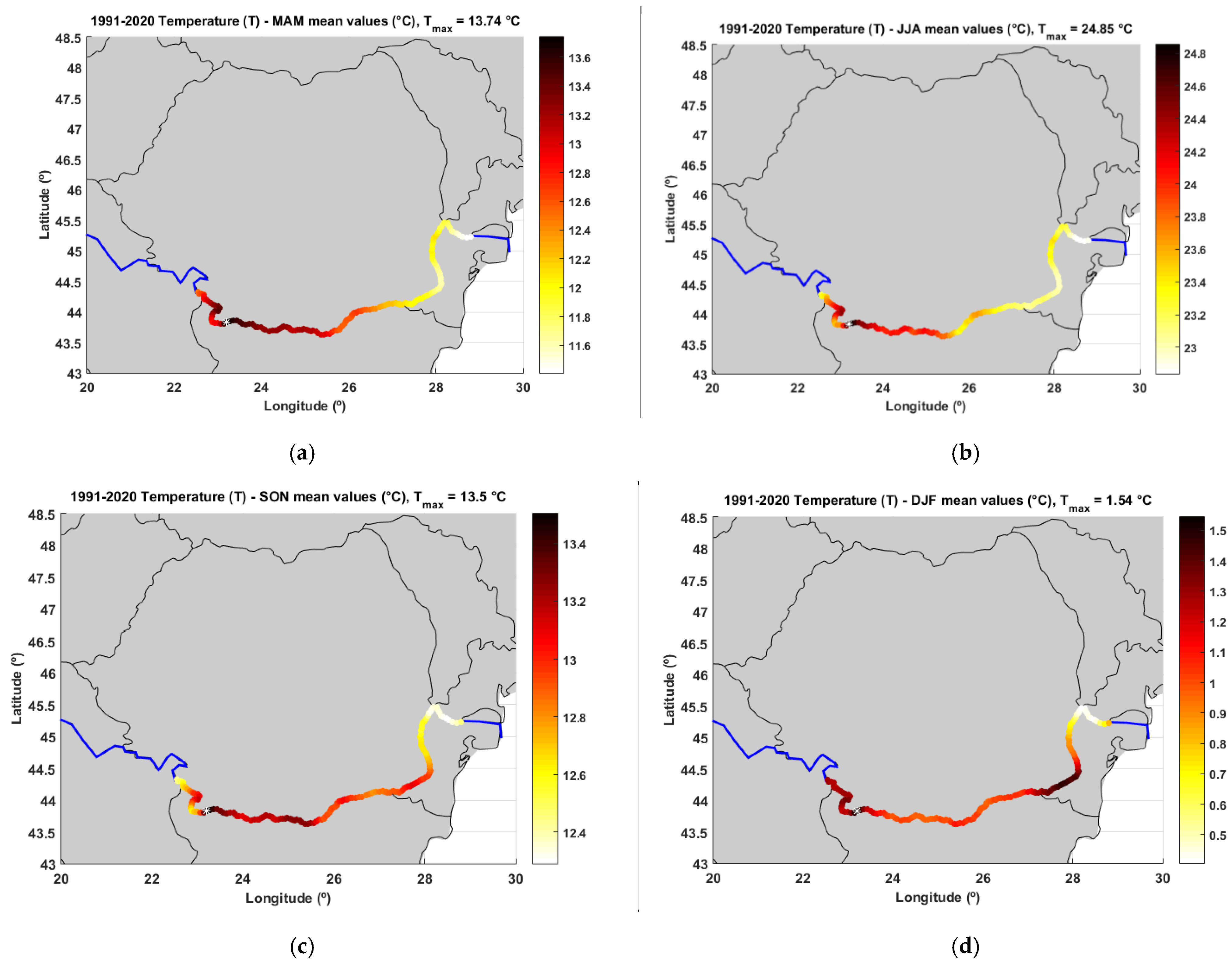
3.2. Air Temperature

The next analysis performed related the air temperature at a 2 m height (T₂). Figure 7a presents the distribution of the maximum air temperature, while Figure 7b the minimum values corresponding to the same process for the 30-year time interval considered (1991–2020). The results showed that the maximum air temperature values are between 38 and 45 °C, while the minimums between −19 and −27 °C. As a paradox, the locations of the minimums and that of the maximums are geographically very close, in the vicinity of the Romanian city of Turnu Măgurele. Figure 8 illustrates the T₂ annual maximum and minimum series together with the corresponding linear regressions and the moving averages. For the maximum temperatures, the trend indicated for a 10-year period is a decrease of about 0.4 °C, while for the minimum, an average enhancement of 0.8 °C was observed for 10 years.

The 99th and 95th percentiles of the air temperature, on the one hand, and the 1st and 5th percentiles, on the other hand, are illustrated in Figure 9. The results indicate that less than 1% of the air temperatures are higher than 35 °C, while more than 95% of the air temperatures have values lower than 30.5 °C. The geographical location of the maximum is in both cases close to the Bulgarian city of Lom. At the same time, less than 1% of the air temperatures are lower than −9.75 °C, while more than 95% of the air temperatures are higher than −4 °C. For the case of the 1st percentile, the geographical location of the minimum is close to the Romanian city of Corabia, while for the 5th percentile, the location of the minimum is in the vicinity of the Ukrainian city of Reni.

Figure 10 presents the average air temperature values along the Lower Danube for the 30-year time interval of 1991–2020, where it can be noticed that these average values are between 11.8 and 13.5 °C and the geographical location of the maximum average value is again close to the Bulgarian city of Lom. The seasonal distributions of the average air temperatures along the Lower Danube for the time interval considered are presented in Figure 11. As expected, the higher mean air temperature values occur in summertime (with average values between 22.8 and 25 °C) and the lower in winter (with average values between 0.5 and 1.5 °C). In spring, the mean air temperature values are in the interval (1.5–13.7) °C, while in autumn, in the interval (12.3–13.5+ °C. For all seasons, the geographical location of the maximum average value is close to the Bulgarian city of Lom.

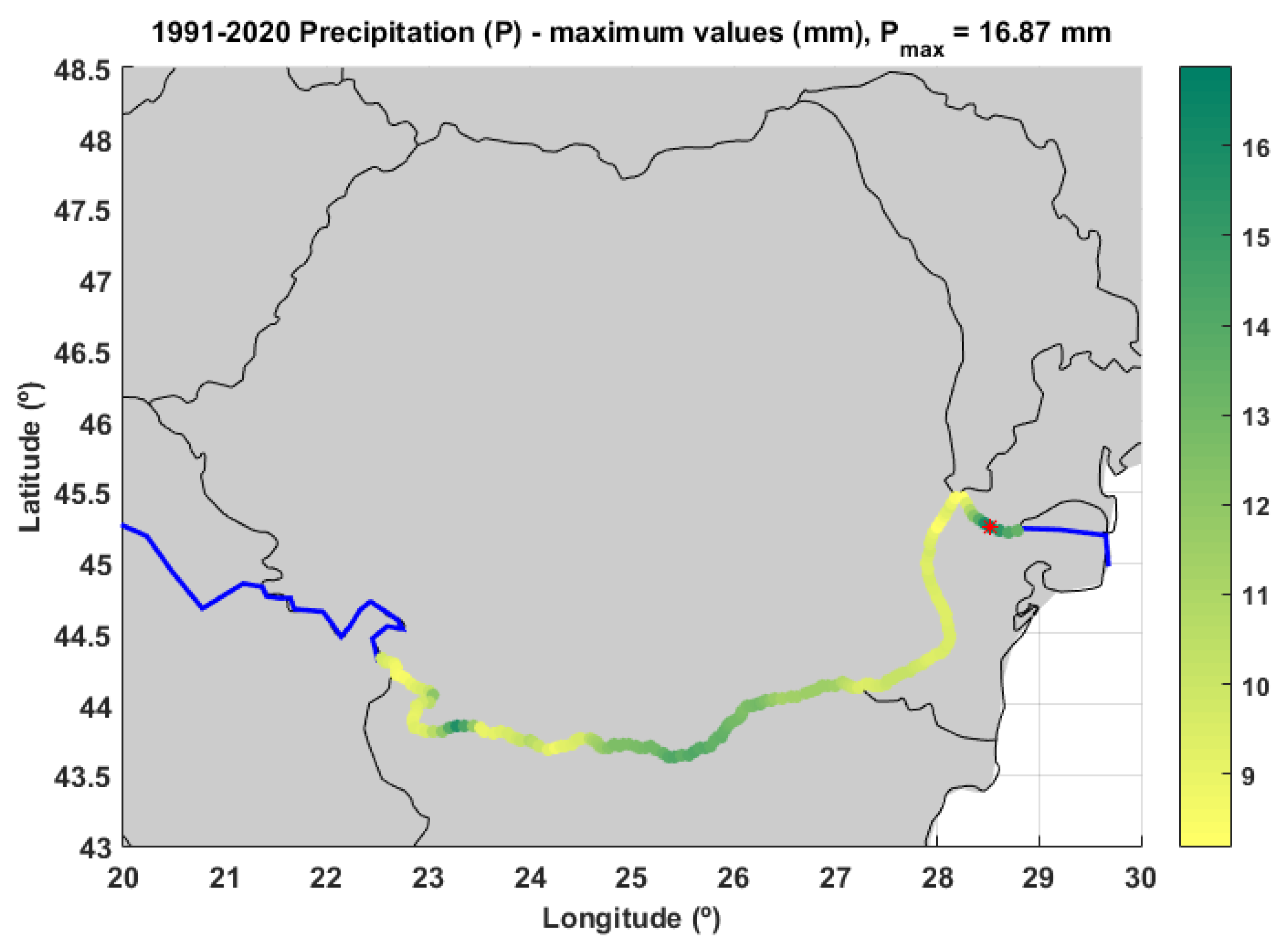
3.3. Precipitation Analysis

The next analysis carried out was related to the precipitation process (P). This represents the precipitation accumulated that falls on the surface and includes both rain and snow. This process is accumulated over a particular time period, which depends on the data extracted. For the reanalysis data, the accumulation period is over the 1 h ending at the validity date and time. The units corresponding to the parameter associated with this process are depth in metres of water equivalent, and it represents the depth if the water would be spread uniformly over the entire grid considered. Figure 12 illustrates the distribution of the maximum precipitation values along the Lower Danube sector considered for the 30-year time interval of 1991–2020. As can be noticed from this figure, the maximum value (almost 17 mm) occurred in the inferior part of the sector, close to the extremity of the sector (the Romanian city of Tulcea). Figure 13 presents the annual maximum series (bars) for this parameter corresponding to the same 30-year time interval considered. In this figure, the linear regression (indicating the trend) and the moving averages are also provided. The slope of the linear regression indicates a clear tendency of a decrease with a value of about 0.5 mm for a decade.

The 99th and 95th percentiles of precipitation along the Lower Danube for the 30-year time interval analysed are presented in Figure 14. The results indicated that less than 1% of the precipitation values are higher than 1.5 mm, while more than 95% are lower than 0.45 mm. Figure 15 presents the average precipitation, where it can be noticed that these are between 0.06 and 0.08 mm. Finally, the seasonal distributions of the average precipitation values along the Lower Danube for the time interval considered are illustrated in Figure 16, where it can be noticed that there are not very high interseasonal variations for this process. For each case presented in Figure 15 and Figure 16, the geographical position of the maximum is represented by a red point.

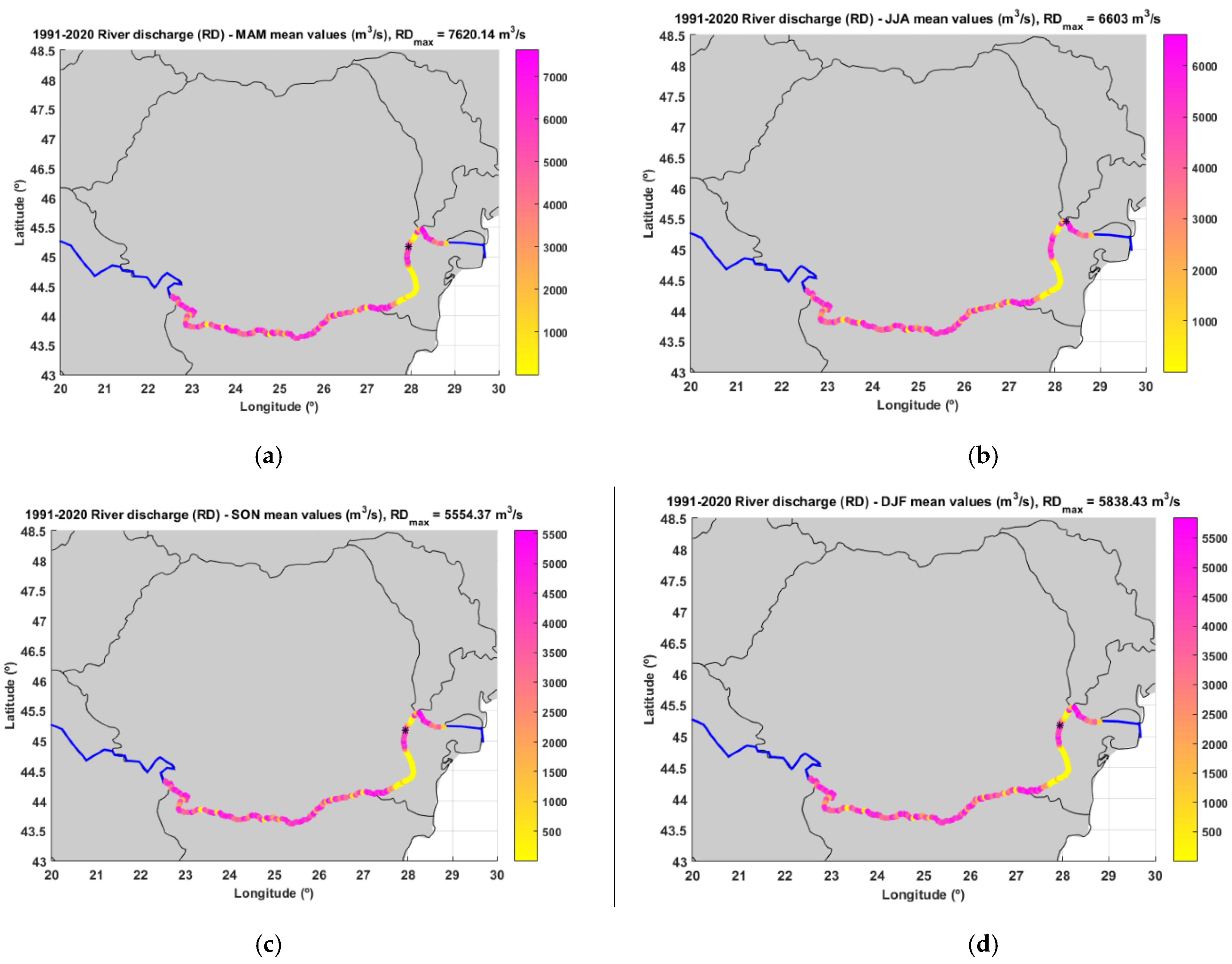
3.4. River Discharge

The last analysis performed relates to the river discharge. The dataset considered for analysis [29] delivers gridded modelled sub-daily and daily hydrological time series forced with meteorological observations. These data are consistent representations of the most-important hydrological variables across the European Flood Awareness System (EFAS). Figure 17 presents the distribution of the maximum river discharge for the 30-year time interval considered (1991–2020). The results show that the maximum river discharge has a wide range of variation along the Lower Danube, with values between 1000 and 20,000 m³/s. Figure 18 illustrates the RD annual maximum and minimum series together with the linear regressions and moving averages. As this figure shows, for the maximum river discharge, the trend indicates a clear enhancement. Thus, for a 10-year period, an average increase greater than 1200 m³/s resulted for this process.

The 99th and 95th percentiles of the river discharge, on the one hand, and the 1st and 5th percentiles, on the other hand, are illustrated in Figure 19. The results indicated that less than 1% of the values related to this process are higher than 13,500 m³/s, while more than 95% of the values are lower than 10,500 m³/s. The geographical location of the maximum is in both cases close to the Ukrainian city of Reni. At the same time, less than 1% of the river discharge values are lower than 2400 m³/s, while more than 95% of the discharges are higher than 3300 m³/s. For the case of the 1st percentile, the geographical location of the maximum is also close to the Ukrainian city of Reni, while for the 5th percentile, the location of the maximum is about 50 km upstream (close to the Romanian city of Braila).

Further on, Figure 20 presents the average values of the river discharge along the Lower Danube for the 30-year time interval of 1991–2020, where it can be noticed that these average values are between 400 and 6400 m³/s, and the geographical location of the maximum average value is again close to the Romanian city of Braila. Finally, the seasonal distributions of the average river discharges along the Lower Danube for the time interval considered are presented in Figure 21. From this figure, it can be noticed that there are not very high interseasonal variations also in the case of this process, the highest average value (about 7600 m³/s) resulting in spring close to the Romanian city of Braila.

Regarding the high spatial variations in terms of the river discharge, it has to be also highlighted that the hydraulic constructions that have been built throughout the years along the river could have a major impact on the trends. Of course, such existing hydraulic constructions are accounted for by the EFAS system, but the on-going projects might affect the future trends.

4. Discussion and Some Statistical Analyses

In the previous section, a quantitative analysis was made concerning the dynamics of four relevant processes along the Lower Danube in the last 30 years. One of the major impacts on inland navigation is the temporal and spatial variability of the hydro meteorological processes mostly related to the water cycle (such as wind speed, temperature, humidity, precipitation, stream flow, etc.). This variability can be quantified through the extreme tails of the environmental data associated with these processes, as presented and discussed in the previous section, but also through the correlation functions (which express how strongly each value depends on the previous values in time of the process and on neighbouring locations). For the extreme tail behaviour, one should focus on the tail of the marginal probability function, as was done in the previous section. However, besides the focus on the occurrence of some high values, an important step for future work is to identify what kind of probability distribution best fits the tail. This can be performed by considering, for example, the results of the recent and extensive work on the extremes of the hydrological cycle of Koutsoyiannis, 2022 [30], where, for the scales and resolutions selected, the so-called Pareto–Burr–Feller distribution seems to well capture most significant water cycle processes. For the correlation function, the most-important behaviours are the so-called fractal (related to small scales) and long-range dependences (related to the large scales), where it has been shown (Dimitriadis et al., 2021) [31] that both of them appear in all the key hydrological cycle processes such as the ones analysed in the present study in both time and space. Since a detailed analysis of the stochastic characteristics will be performed in future work, at this point, some statistical parameters were evaluated concerning the spatial coefficient of variation and the cross-correlation between each pair of analysed processes (wind, temperature, precipitation, and river discharge). The spatial coefficient of variation (SCV_ROI) in a region of interest (ROI) is calculated as the ratio of the standard deviation ${\sigma }_{ROI}$ to the mean value ${\mu }_{ROI}$ [32]:

$$SC{V}_{ROI}=\frac{{\sigma }_{ROI}}{{\mu }_{ROI}}·100$$

(5)

where the mean is computed with the relation given in Equation (4), while the standard deviation is

$$\sigma =\sqrt{\frac{1}{N}{\sum }_{i=1}^N\left(X_i-\overline{X}\right)}$$

(6)

This gives information on the average variability of a dataset. It indicates how far each value lies from the mean. A high standard deviation means that the values are generally far from the mean, while a low standard deviation that the values are clustered close to the mean. A higher SCV value indicates a greater dispersion. The coefficient of variation is useful as it is dimensionless (i.e., independent of the unit in which the measurement was taken) and, thus, comparable between datasets with different units or widely different means. In this case, the ROI was along the Lower Danube River. For the four processes analysed (wind, temperature, precipitation, and river discharge),

Table 1. Spatial coefficients of variation corresponding to the 30-year time interval (1991–2020) in the Lower Danube for the processes analysed.

Process	Wind Speed (U)	Temperature (T)	River Discharge (RD)	Precipitation (P)
SCVROI (%)	7.88	2.76	57.43	8.44

presents the values of the spatial coefficients of variation corresponding to the 30-year time interval (1991–2020) in the Lower Danube. As expected, the highest variations correspond to the river discharge (57.43%), while the lowest to the air temperature (2.76%). Regarding the wind speed and precipitation, the values of this indicator are quite similar (7.88% and 8.44%, respectively).

Another indicator evaluated was the cross-correlation between two processes. This is computed considering Equation (7), which gives the cross-correlation between two generic signals denoted by x(k) and y(k) [32]:

$$c\left(\tau \right)=\frac{1}{N}{\displaystyle \sum _{k=1}^{N-\tau }\frac{\left[x\left(k\right)-{\mu }_k\right]\left[y\left(k+\tau \right)-{\mu }_k\right]}{{\sigma }_x{\sigma }_y}}$$

(7)

where μ_x and μ_y are the mean values of x and y, respectively, while σ_x and σ_y are the corresponding standard deviations; τ represents the time lag between the signals (in this work, τ = 0), and c(τ) gives their correspondence. The values of c(τ) are between −1 and 1, the unit value indicating a perfect correspondence.

The cross-correlation coefficients between each pair of two meteorological processes along the Lower Danube are presented in Figure 22. In order to design these variation diagrams, in each geographical point along the Lower Danube, the cross-correlation between the temporal series was computed for each pair of data corresponding to two processes (P and T; U and T; U and P). According to [32], the degree of correlation is extremely strong if the coefficient is in the range (0.8–1), strong for (0.6–0.8), medium for values in the range (0.4–0.6), weak for (0.2–0.4)], and very weak for values in the range (0–0.2). From this perspective, the results presented in Figure 22 indicate a very weak correlation between the three meteorological processes analysed, the highest correlation values (between 0.1 and 0.15) resulting for wind speed and precipitation, while the lowest (with values between −0.12 and 0.02) resulting for wind speed and temperature. Regarding the cross-correlation results, a recent analysis (with very similar results, but on a global scale) performed by Koskinas [33] should be mentioned at this point, where a weak cross-correlation (below 0.2) was traced between precipitation and wind and precipitation and temperature, whereas larger values (but with also higher variations) were traced between temperature and wind.

5. Conclusions

The objective of the present work was to analyse the last 30 years of dynamics (1991–2020) of four relevant environmental processes (three meteorological and one hydrological) along the Lower Danube. From this perspective, the processes analysed were: the wind speed at a 10 m height, the air temperature at a 2 m height, precipitation, and river discharge. Since the target of the work was to support inland navigation, the emphasis was placed on the extreme events indicating the maximum values of the processes analysed and the geographical locations where such extreme occurrences are more probable.

From this perspective, the main findings resulting from the 30-year analysis carried out in the present work can be outlined as follows:

The maximum wind speed values (not higher than 14 m/s) appeared to be considerably lower than in the neighbouring marine coastal areas [34], and the analysis performed indicated no significant changes in the last three decades along the Lower Danube in relation to this process, unlike in the marine environment or other areas.

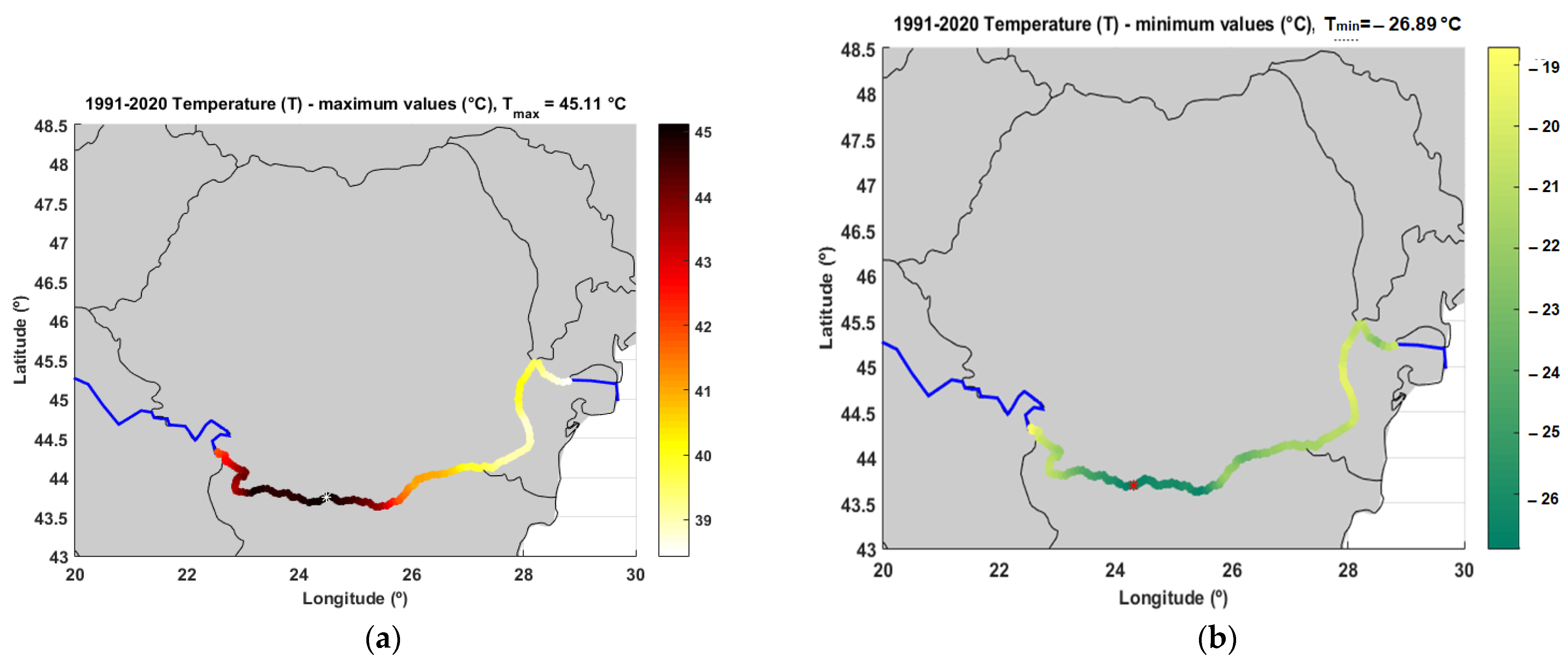
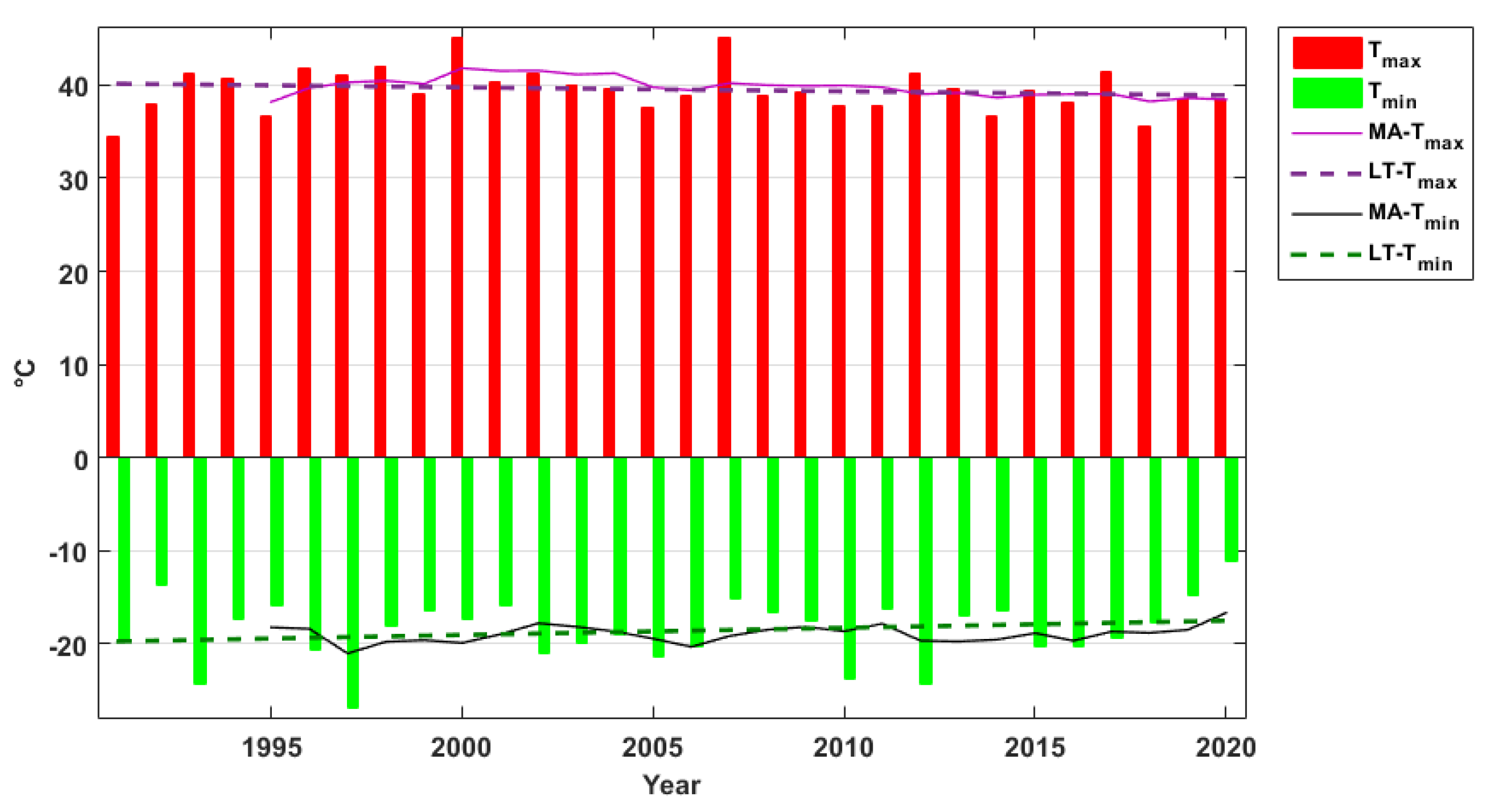
• The air temperature values along the Lower Danube for the 30-year time period considered were in the interval [–27, 45] °C. In this case, a small tendency of the decreasing of the maximum values was noticed together with a clearer tendency of an increase for the minimum temperatures, with an average value of 0.8 °C per decade, a trend that looks similar also for the average air temperatures. This trend was in line with some other results presented in the literature, as for example those from [35], according to which the minimum temperature seemed to globally increase more than the maximum one. At this point, it should also be highlighted that the datasets analysed did not provide the water temperature, which represents another important process, although its significance for inland navigation is not very high. Methods to estimate the air–water temperature dependency in the Lower Danube were designed, fit with a logistic function with a good approximation. Such correlations may help in predicting water temperature as a function of satellite-measured air temperature [36].
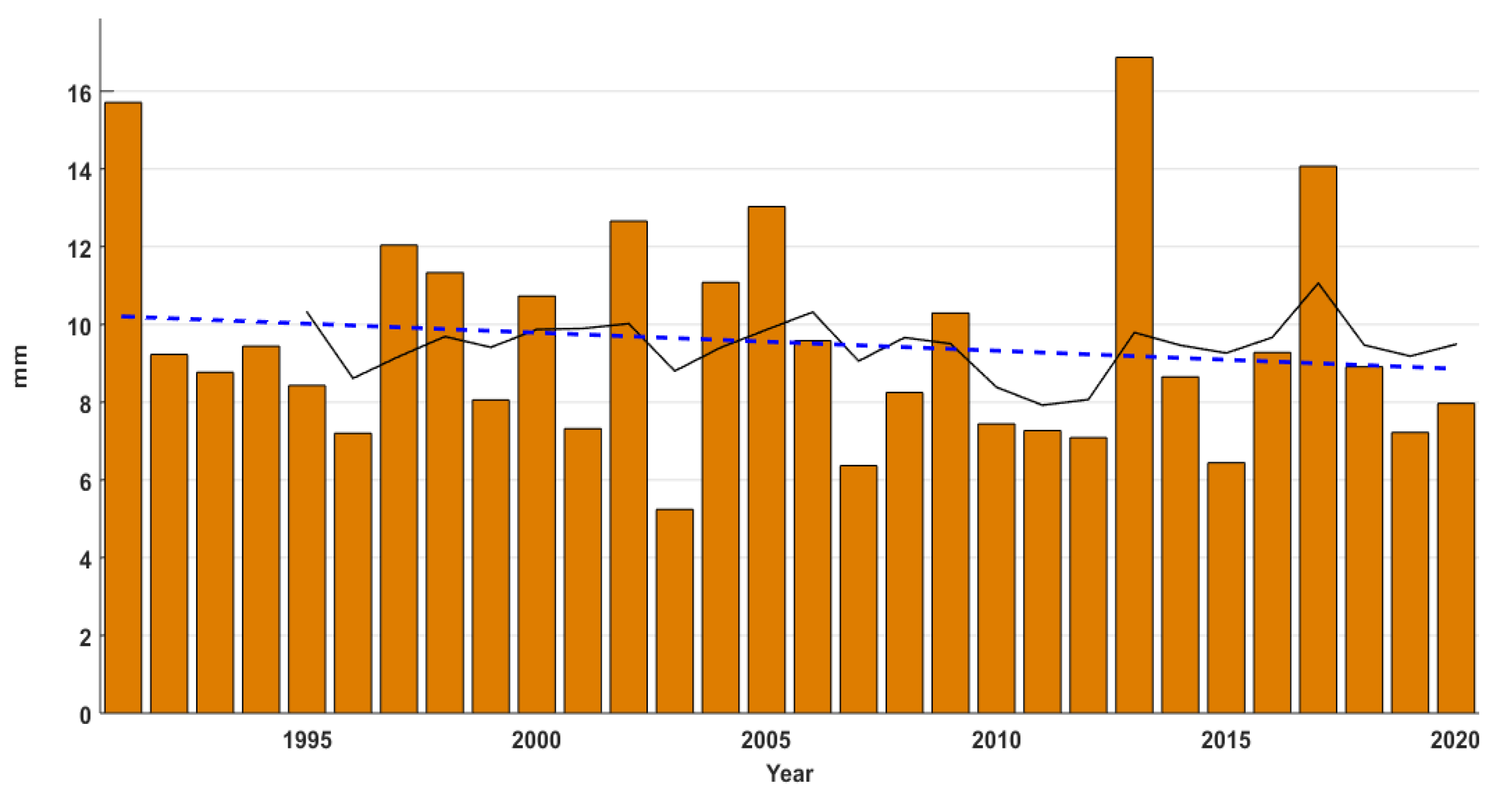
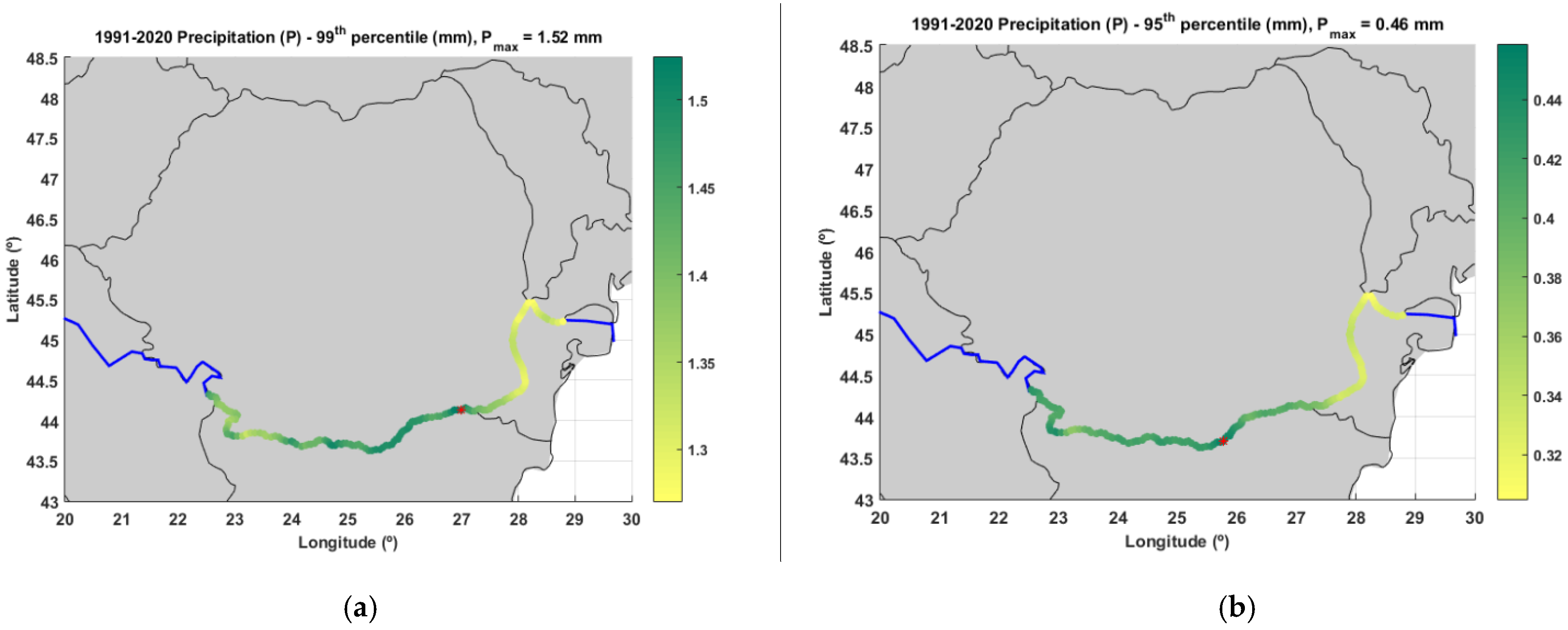
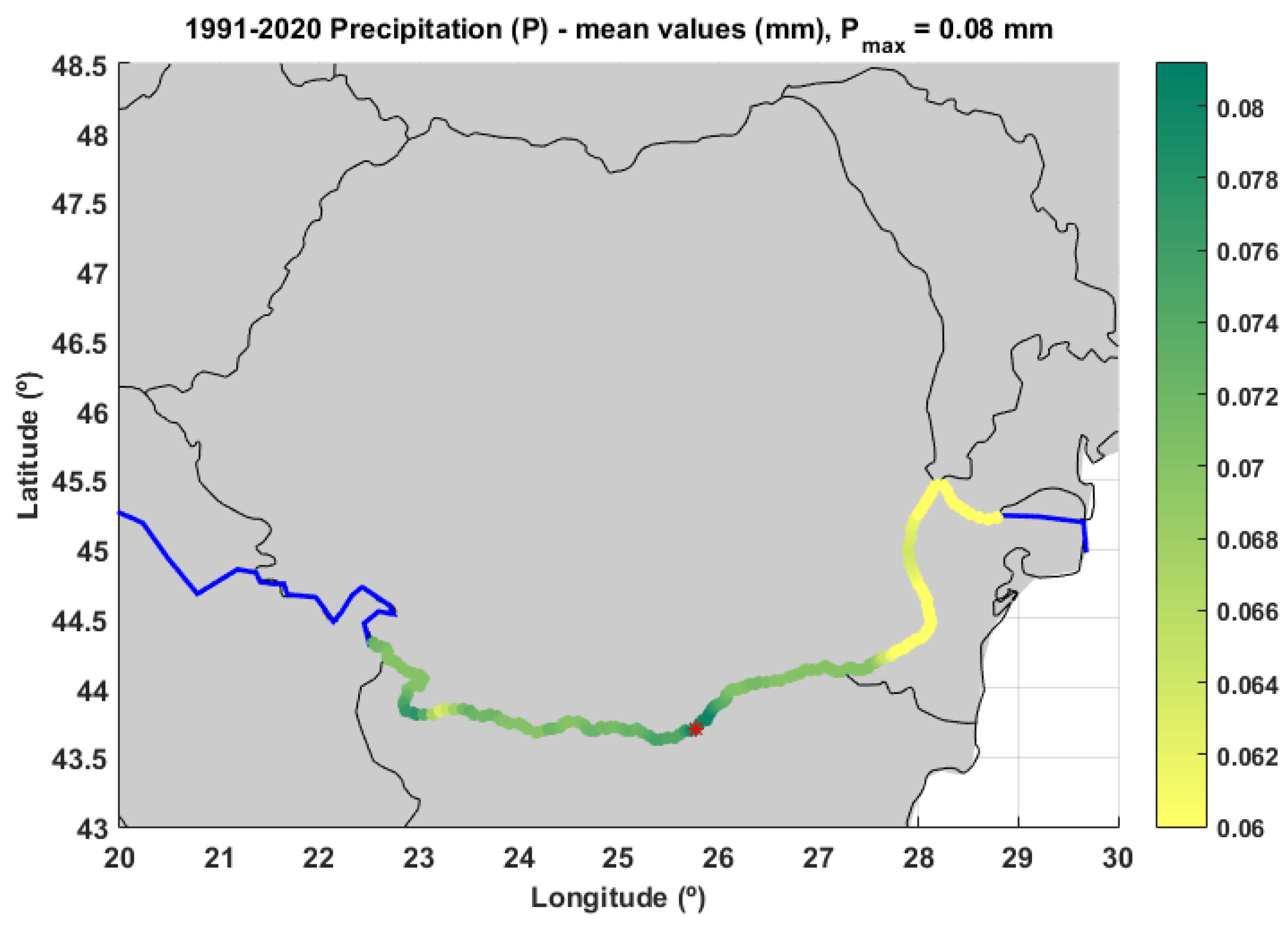
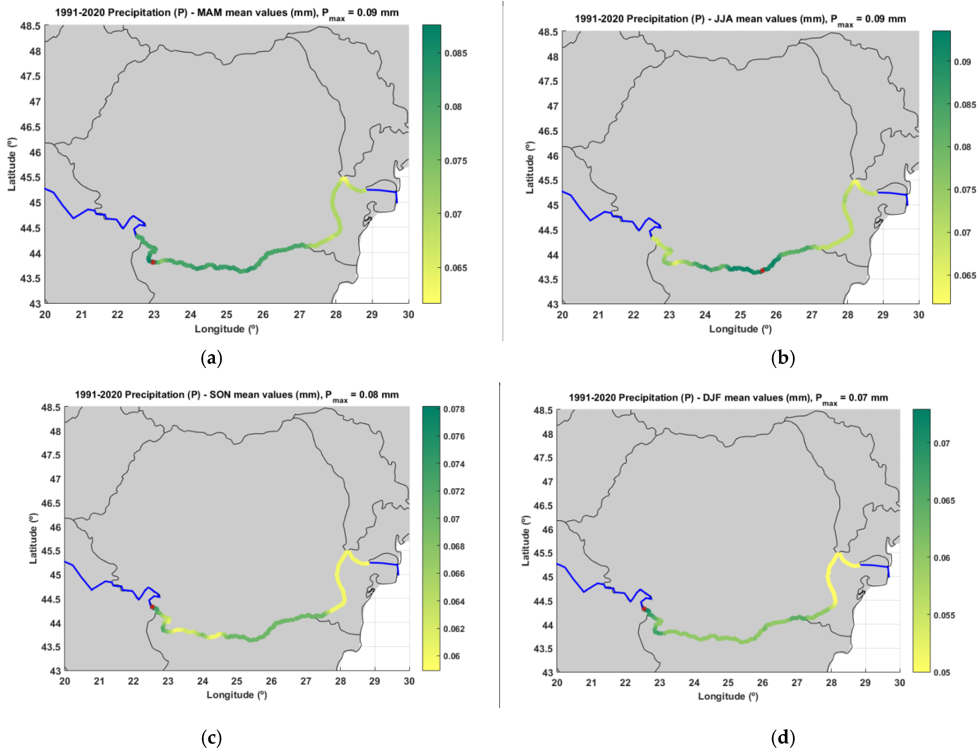
• The precipitation analysis along the Lower Danube indicated a very clear decreasing trend of about 0.5 mm per decade, while the maximum value of the parameter associated with this process for the 30-year period analysed was about 17 mm, and the corresponding location was close to the lower limit of the Danube sector considered (the Romanian city of Tulcea). At this point, it has to be highlighted also that, in the case of precipitation, the river is fed also by the inflow from the catchment and not only by precipitation that has fallen on the river surface. On the other hand, the values of this process, together with the wind speed and air temperature, might be relevant to the navigation conditions and other human activities taking place along this sector of the Danube.
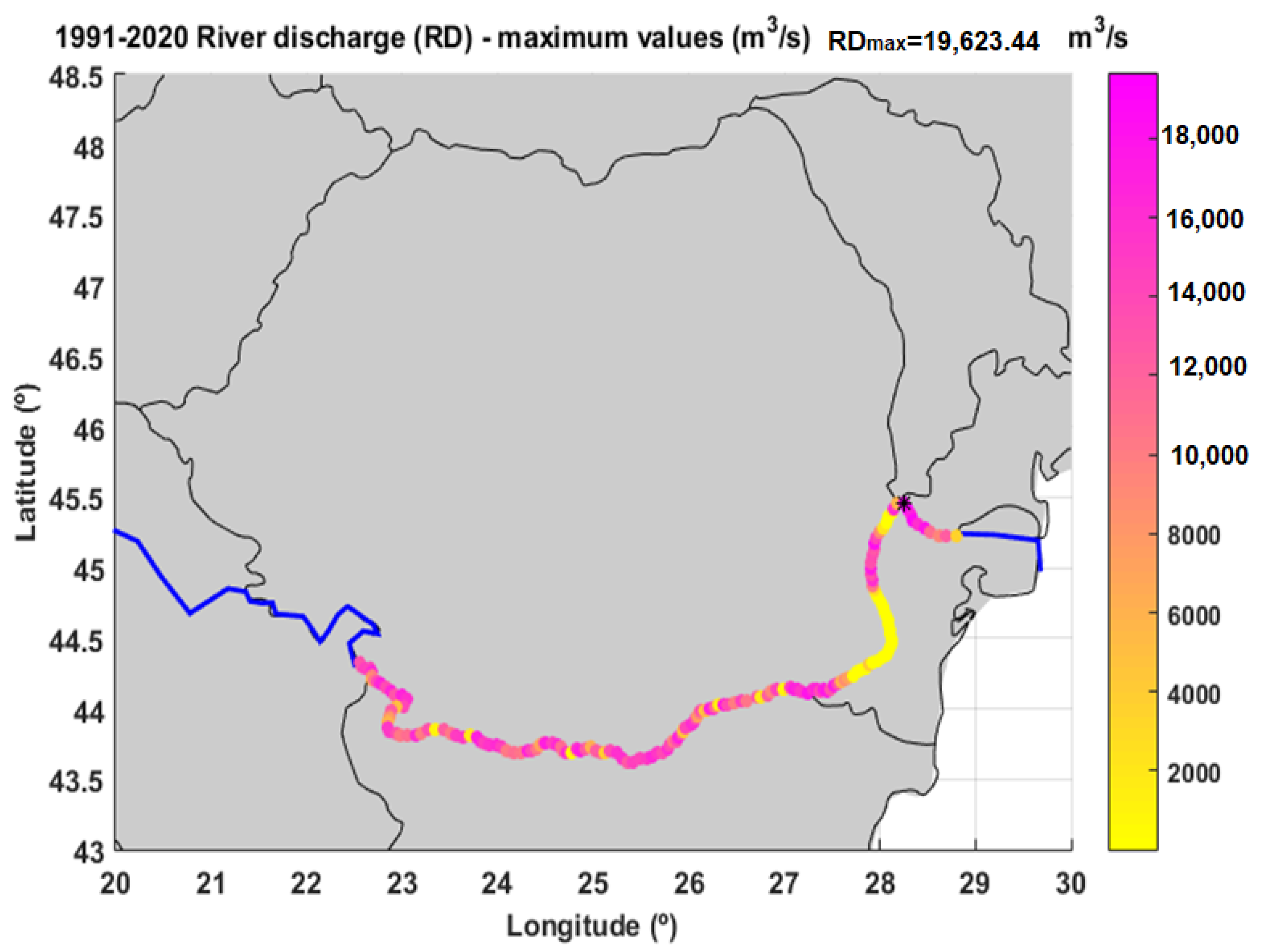
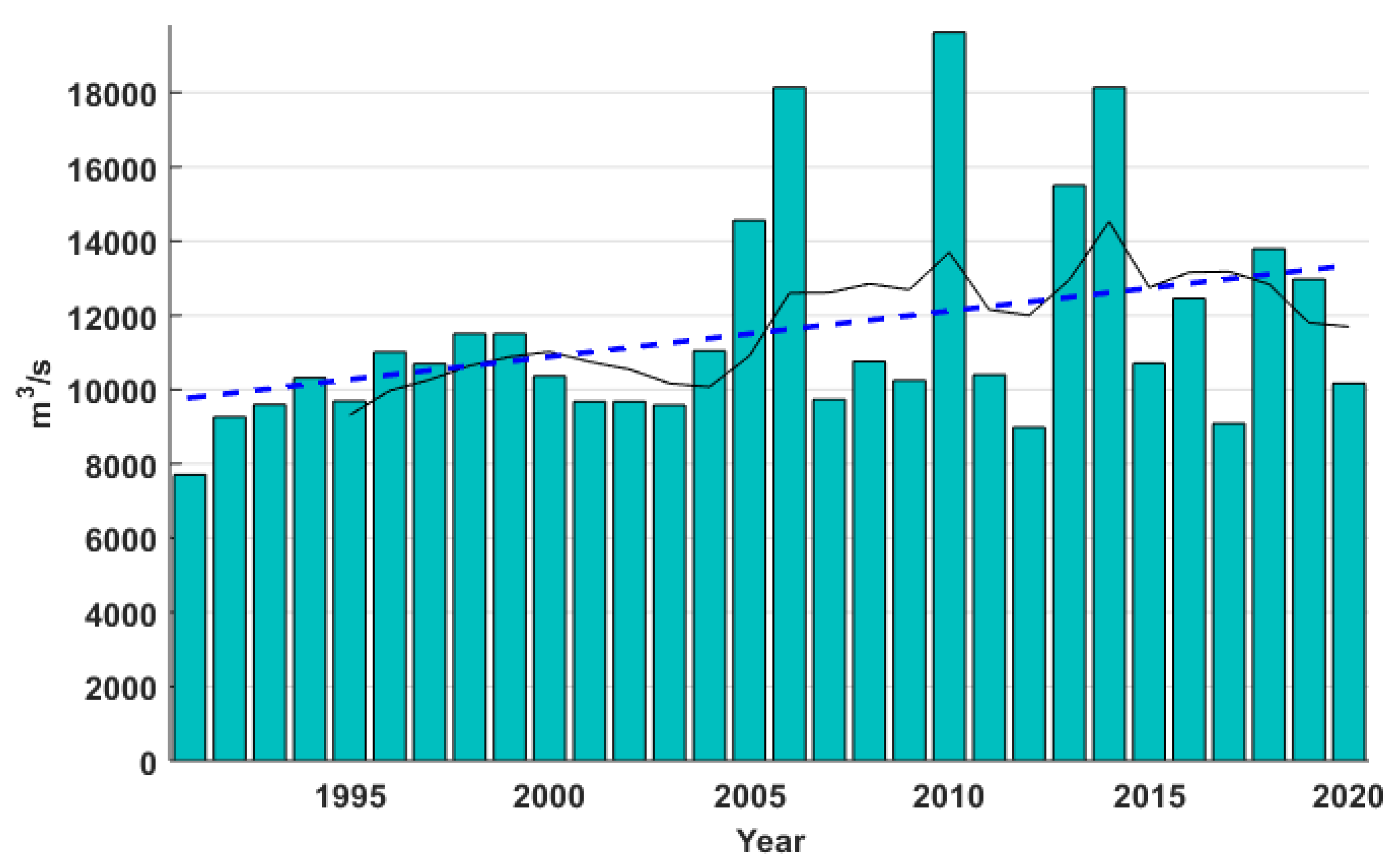
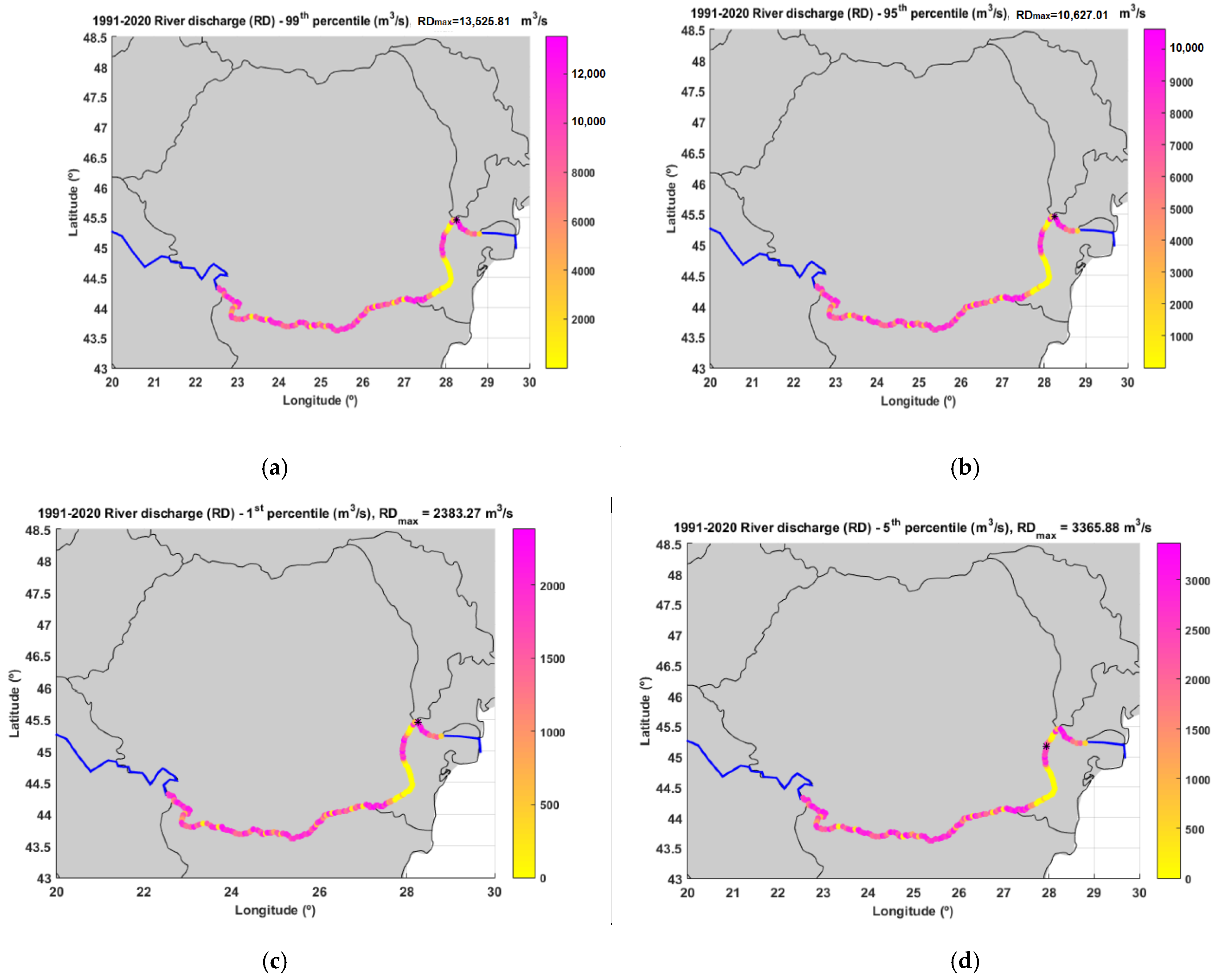
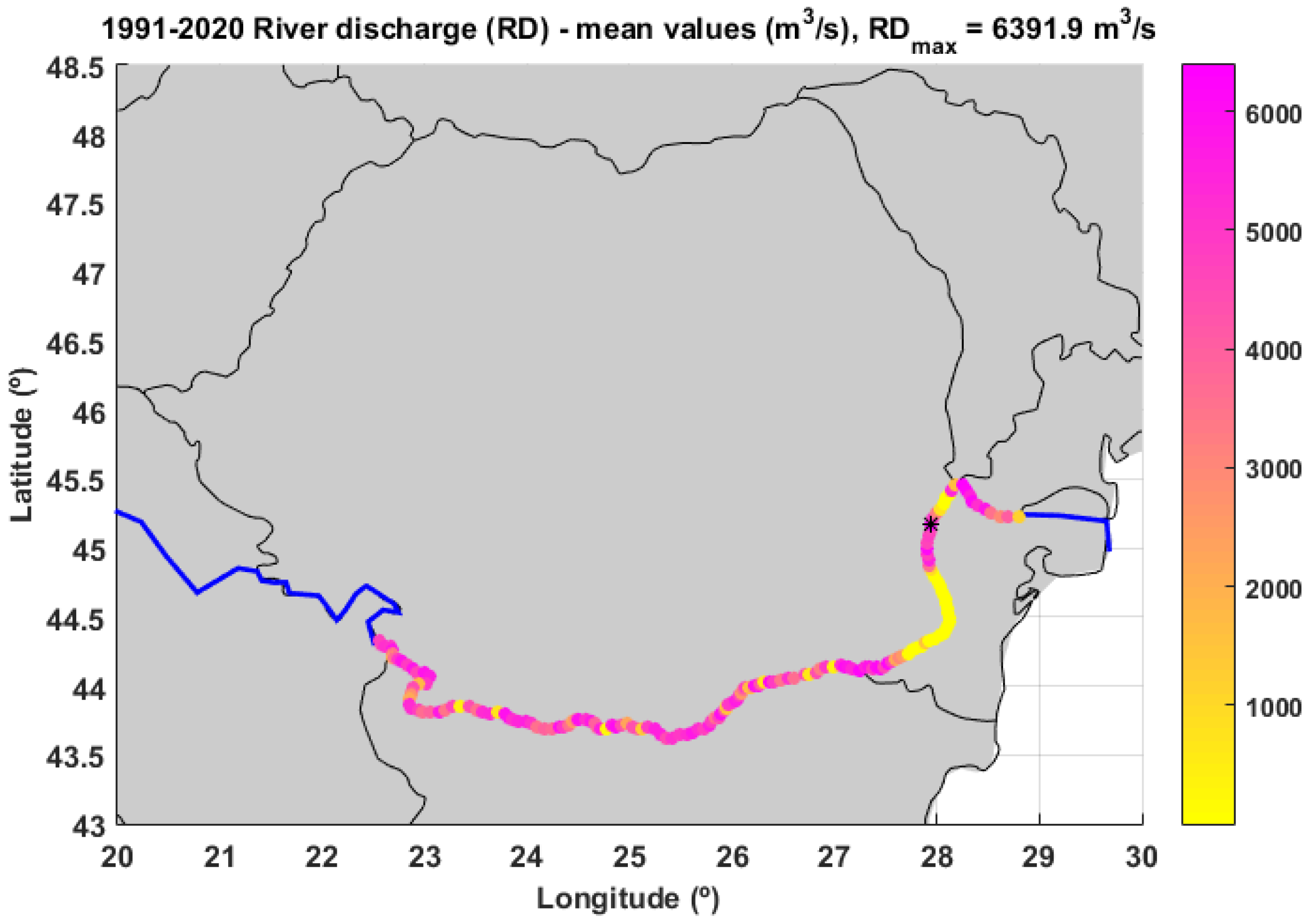
• The river discharge has a very high geographical variability along the Lower Danube sector, with maximum values between 1000 and 20,000 m³/s. The results of the analysis indicated also a constant tendency of enhancement for the values of the maximum river discharge with an average increase per decade higher than 1200m³/s.
• The statistical analysis performed indicated that the higher spatial variability corresponded to the river discharge (57.4%), while the lowest to the air temperature (2.8). For the wind speed and precipitation, the spatial variability had very similar values (7.9% and 8.4%, respectively).
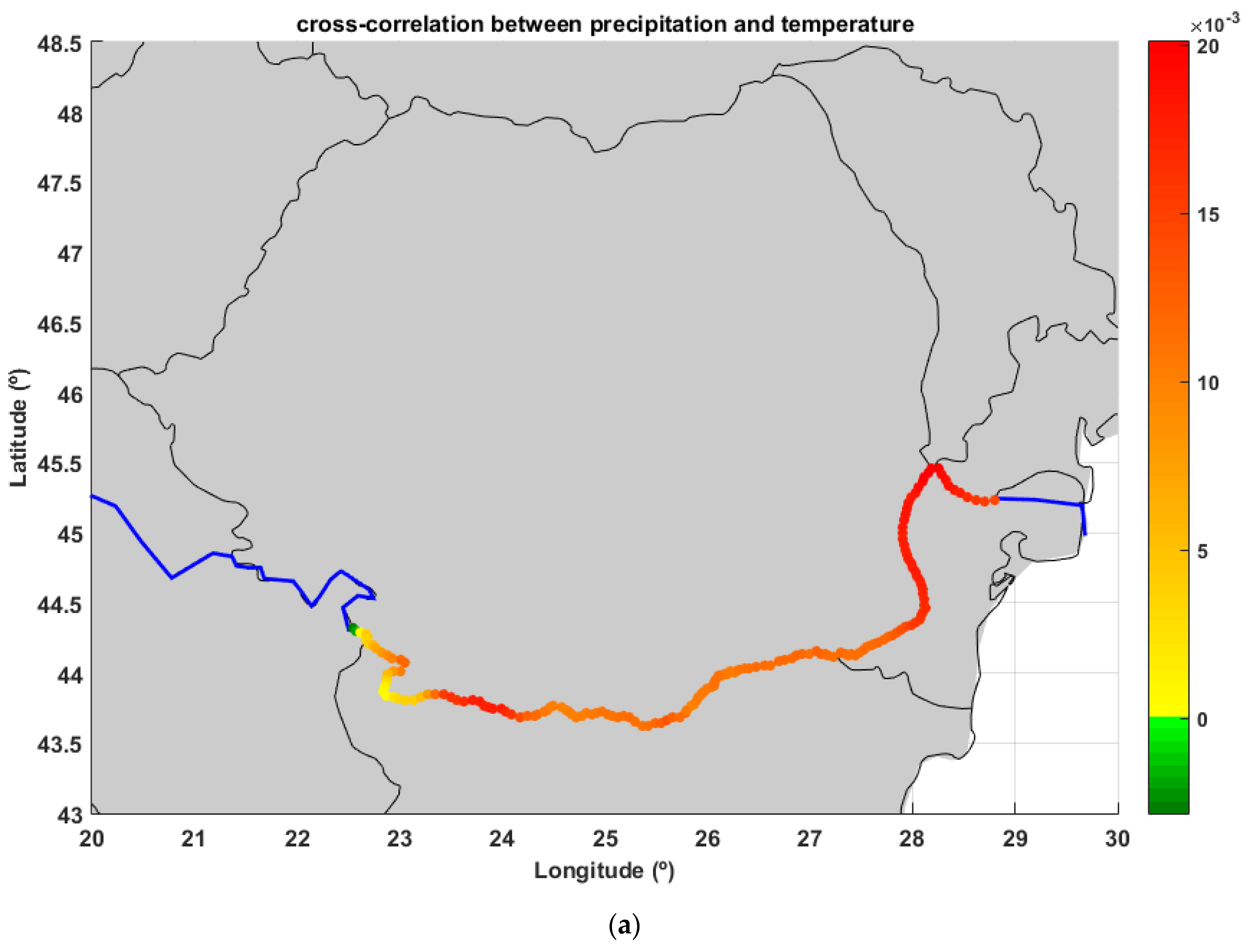
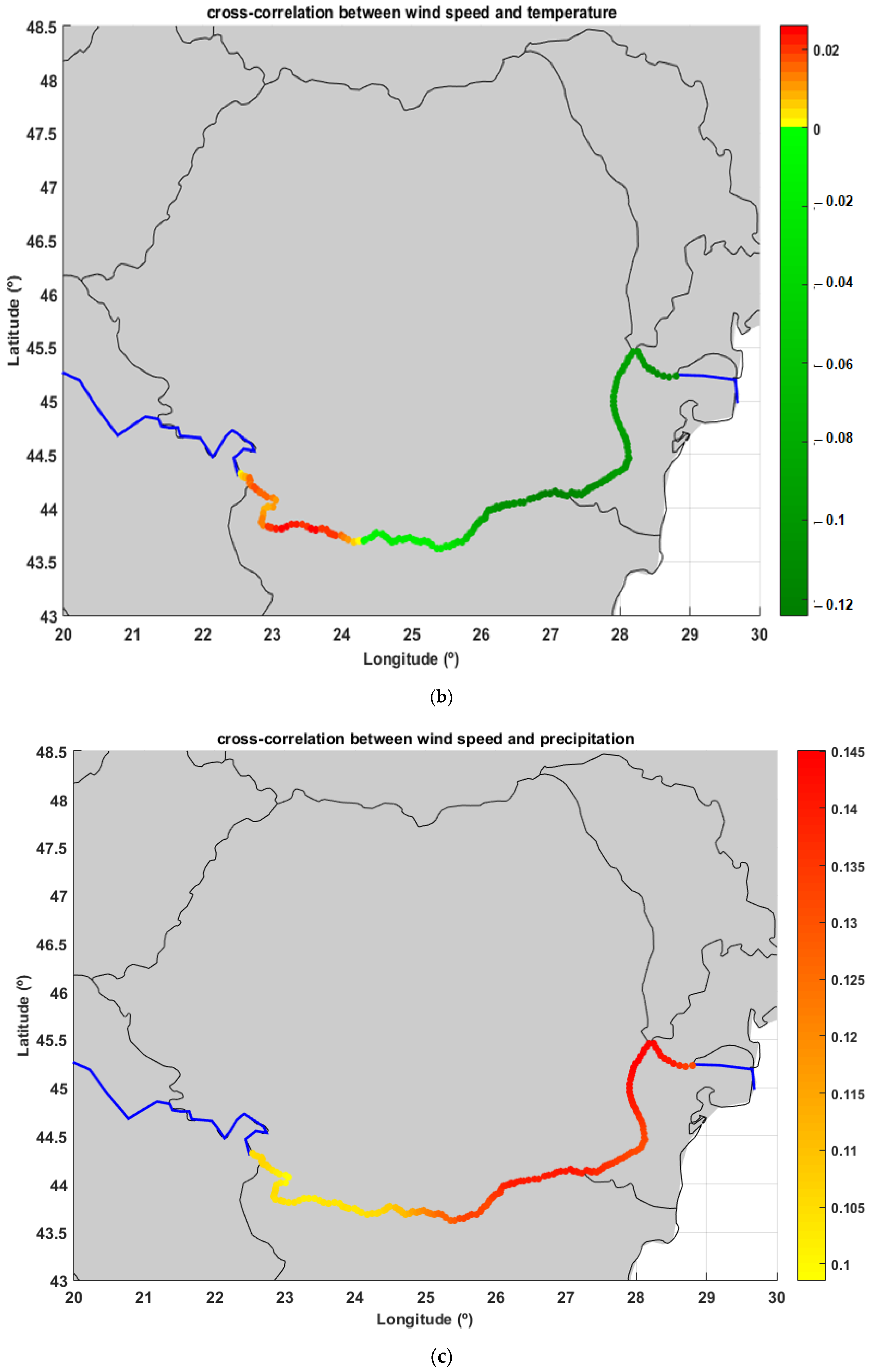
• The results indicated an extremely low correlation between the three meteorological processes analysed (wind speed, air temperature, and precipitation), the highest correlation values (between 0.1 and 0.15) resulting for wind speed and precipitation, while the lowest (with values between 0.12 and 0.02) resulting for wind speed and temperature.

It has to be also highlighted at this point that, concerning the estimated trends, there is a large literature that shows that, in order to properly estimate the trend, a robust stochastic test must be considered. An enhanced discussion in this direction is provided by Iliopoulou and Koutsoyiannis [37] in relation to the estimation of the trends, as well as the results for the extreme precipitation.

Finally, it can be concluded that the processes analysed are also significantly influenced by factors outside the geographical boundary of the Danube. For example, the temperature and wind along the Danube are driven mainly by large-scale climatic processes. At the same time, there might also be some concerns about using the reanalysis data (ERA5) as the major source of information. From this perspective, for a more reliable evaluation, local in situ measurements will also be considered in future work in certain locations. On the other hand, it can be also underlined that the meteorological processes analysed are spatial in nature, and their variability along the Lower Danube sector represents a significant issue, especially if we refer to inland navigation, harbour operations, or hydro technical works along the river. Hence, the present work provided a general and more comprehensive perspective of the recent dynamics of the environmental matrix along the Lower Danube sector.

The work is still ongoing, and together with more detailed statistical analyses, an important next step is to consider also the analysis of some observed information inside the study area, especially in those locations identified in the present work as having a higher incidence of the extreme values. Further on, another important direction to be explored is related to the assessment of the expected dynamics of the main environmental processes resulting from the climatic projections developed under various Representative Concentration Pathway (RCP) and Shared Socioeconomic Pathway (SSP) scenarios in order to identify the possible and most-probable future climatic trends along the Lower Danube.

References

1. Pinka, P.G.; Penčev, P.G. Danube River. Encyclopedia Britannica. 23 August 2022. Available online: https://www.britannica.com/place/Danube-River (accessed on 2 February 2023).
2. ICPDR 2022, The International Commission for the Protection of the Danube River. Available online: https://www.icpdr.org/main/ (accessed on 2 February 2023).
3. Rouholahnejad Freund, E.; Abbaspour, K.C.; Lehmann, A. Water Resources of the Black Sea Catchment under Future Climate and Landuse Change Projections. Water 2017, 9, 598. [Google Scholar] [CrossRef] [Green Version]
4. Rusu, E. Modelling of wave-current interactions at the mouths of the Danube. J. Mar. Sci. Technol. 2010, 15, 143–159. [Google Scholar] [CrossRef]
5. Banescu, A.; Arseni, M.; Georgescu, L.P.; Rusu, E.; Iticescu, C. Evaluation of different simulation methods for analyzing flood scenarios in the Danube Delta. Appl. Sci. 2020, 10, 8327. [Google Scholar] [CrossRef]
6. Stanica, A.; Panin, N. Present evolution and future predictions for the deltaic coastal zone between the Sulina and Sulina and Sf. Gheorghe Danube river mouths (Romania). Geomorphology 2009, 107, 41–46. [Google Scholar] [CrossRef]
7. Lazar, L.; Rodino, S.; Pop, R.; Tiller, R.; D’Haese, N.; Viaene, P.; De Kok, J.-L. Sustainable Development Scenarios in the Danube Delta—A Pilot Methodology for Decision Makers. Water 2022, 14, 3484. [Google Scholar] [CrossRef]
8. Eder, M.; Perosa, F.; Hohensinner, S.; Tritthart, M.; Scheuer, S.; Gelhaus, M.; Cyffka, B.; Kiss, T.; Van Leeuwen, B.; Tobak, Z.; et al. How Can We Identify Active, Former, and Potential Floodplains? Methods and Lessons Learned from the Danube River. Water 2022, 14, 2295. [Google Scholar] [CrossRef]
9. Stagl, J.C.; Hattermann, F.F. Impacts of Climate Change on the Hydrological Regime of the Danube River and Its Tributaries Using an Ensemble of Climate Scenarios. Water 2015, 7, 6139–6172. [Google Scholar] [CrossRef]
10. Stagl, J.C.; Hattermann, F.F. Impacts of Climate Change on Riverine Ecosystems: Alterations of Ecologically Relevant Flow Dynamics in the Danube River and Its Major Tributaries. Water 2016, 8, 566. [Google Scholar] [CrossRef] [Green Version]
11. Maternová, A.; Materna, M.; Dávid, A. Revealing Causal Factors Influencing Sustainable and Safe Navigation in Central Europe. Sustainability 2022, 14, 2231. [Google Scholar] [CrossRef]
12. Aszódi, A.; Biró, B.; Adorján, L.; Dobos, Á.C.; Illés, G.; Tóth, N.K.; Zagyi, D.; Zsiboras, Z.T. Comparative analysis of national energy strategies of 19 European countries in light of the green deal’s objectives. Energy Convers. Manag. X 2021, 12, 100136. [Google Scholar] [CrossRef]
13. Probst, E.; Mauser, W. Climate Change Impacts on Water Resources in the Danube River Basin: A Hydrological Modelling Study Using EURO-CORDEX Climate Scenarios. Water 2023, 15, 8. [Google Scholar] [CrossRef]
14. ICPDR 2013, Hydropower Case Studies and Good Practice Example. Available online: https://www.icpdr.org/main/sites/default/files/nodes/documents/annex_-_case_studies_and_good_practice_examples_final.pdf (accessed on 2 February 2023).
15. Change 2022: Impacts, Adaptation and Vulnerability n.d. Available online: https://www.ipcc.ch/report/ar6/wg2/ (accessed on 4 January 2023).
16. Joint European Action for More Affordable, Secure Energy. European Commission—European Commission n.d. Available online: https://ec.europa.eu/commission/presscorner/detail/en/ip_22_1511 (accessed on 30 January 2023).
17. Camuc, M.; Calmuc, V.; Arseni, M.; Topa, C.; Timofti, M.; Georgescu, L.P.; Iticescu, C. A Comparative Approach to a Series of Physico-Chemical Quality Indices Used in Assessing Water Quality in the Lower Danube. Water 2020, 12, 3239. [Google Scholar] [CrossRef]
18. Radu, C.; Manoiu, V.-M.; Kubiak-Wójcicka, K.; Avram, E.; Beteringhe, A.; Craciun, A.-I. Romanian Danube River Hydrocarbon Pollution in 2011–2021. Water 2022, 14, 3156. [Google Scholar] [CrossRef]
19. Popa, P.; Murariu, G.; Timofti, M.; Georgescu, L.P. Multivariate Statistical Analyses of Danube River Water Quality at Galati, Romania. Environ. Eng. Manag. J. 2018, 17, 1249–1266. [Google Scholar]
20. Calmuc, V.A.; Calmuc, M.; Arseni, M.; Topa, C.M.; Timofti, M.; Burada, A.; Iticescu, C.; Georgescu, L.P. Assessment of Heavy Metal Pollution Levels in Sediments and of Ecological Risk by Quality Indices, Applying a Case Study: The Lower Danube River, Romania. Water 2021, 13, 1801. [Google Scholar] [CrossRef]
21. Iticescu, C.; Georgescu, L.P.; Topa, C.; Murariu, G. Monitoring the Danube Water Quality Near the Galati City. J. Environ. Prot. Ecol. 2014, 15, 30–38. [Google Scholar]
22. Romanescu, G.; Mihu-Pintilie, A.; Stoleriu, C.C.; Carboni, D.; Paveluc, L.E.; Cimpianu, C.I. A Comparative Analysis of Exceptional Flood Events in the Context of Heavy Rains in the Summer of 2010: Siret Basin (NE Romania) Case Study. Water 2018, 10, 216. [Google Scholar] [CrossRef] [Green Version]
23. Tomić, N.; Marjanović, M. Towards a Better Understanding of Motivation and Constraints for Domestic Geotourists: The Case of the Middle and Lower Danube Region in Serbia. Sustainability 2022, 14, 3285. [Google Scholar] [CrossRef]
24. Negm, A.; Zaharia, L.; Toroimac, G.I. The Lower Danube River Hydro-Environmental Issues and Sustainability; Springer: Berlin/Heidelberg, Germany, 2022; ISBN 978-3-031-03864-8. [Google Scholar]
25. ShipTraffic.net. Available online: http://www.shiptraffic.net/2001/04/danube-river-ship-traffic.html?full_screen=yes&map=vf (accessed on 2 February 2023).
26. ICPDR 2023, The Future of the Danube River Basin. Available online: https://icpdr.org/main/publications/future-danube-river-basin (accessed on 3 February 2023).
27. ERA5 Hourly Data on Single Levels from 1959 to Present. Available online: https://cds.climate.copernicus.eu/cdsapp#!/dataset/reanalysis-era5-single-levels?tab=overview (accessed on 25 January 2023).
28. Onea, F.; Rusu, E. Sustainability of the Reanalysis Databases in Predicting the Wind and Wave Power along the European Coasts. Sustainability 2018, 10, 193. [Google Scholar] [CrossRef] [Green Version]
29. River Discharge and Related Historical Data from the European Flood Awareness System. Available online: https://cds.climate.copernicus.eu/cdsapp#!/dataset/efas-historical?tab=form (accessed on 1 February 2023).
30. Koutsoyiannis, D. Stochastics of Hydroclimatic Extremes—A Cool Look at Risk, 2nd ed.; Kallipos Open Academic Editions: Athens, Greece, 2022; 346p, ISBN 978-618-85370-0-2. [Google Scholar] [CrossRef]
31. Dimitriadis, P.; Koutsoyiannis, D.; Iliopoulou, T.; Papanicolaou, P. A global-scale investigation of stochastic similarities in marginal distribution and dependence structure of key hydrological-cycle processes. Hydrology 2021, 8, 59. [Google Scholar] [CrossRef]
32. Wei, X.; Zhang, H.; Gong, X.; Wei, X.; Dang, C.; Zhi, T. Intrinsic cross-correlation analysis of hydro-meteorological data in the Loess Plateau, China. Int. J. Environ. Res. Public Health 2020, 17, 2410. [Google Scholar] [CrossRef] [PubMed] [Green Version]
33. Koskinas, A.; Zaharopoulou, E.; Pouliasis, G.; Deligiannis, I.; Dimitriadis, P.; Iliopoulou, T.; Mamassis, N.; Koutsoyiannis, D. Estimating the Statistical Significance of Cross–Correlations between Hydroclimatic Processes in the Presence of Long–Range Dependence. Earth 2022, 3, 1027–1041. [Google Scholar] [CrossRef]
34. Onea, F.; Rusu, E. Wind energy assessments along the Black Sea basin. Meteorol. Appl. 2014, 21, 316–329. [Google Scholar] [CrossRef]
35. Glynis, K.; Iliopoulou, T.; Dimitriadis, P.; Koutsoyiannis, D. Stochastic investigation of daily air temperature extremes from a global ground station network. Stoch. Environ. Res. Risk Assess. 2021, 35, 1585–1603. [Google Scholar] [CrossRef]
36. Gogoase-Nistorean, D.E.; Ionescu, C.S.; Opris, I. Models to estimate river temperature. Example for Danube, at Oltenița in the context of climate change and anthropic impact. E3S Web Conf. 2021, 286, 04003. [Google Scholar] [CrossRef]
37. Iliopoulou, T.; Koutsoyiannis, D. Projecting the future of rainfall extremes: Better classic than trendy. J. Hydrol. 2020, 588, 125005. [Google Scholar] [CrossRef]
Figure 1. Map of the Lower Danube sector and locations of the main river and adjacent maritime ports. Figure processed by the authors using information from [25].
Sustainability 15 06087 g001
Figure 2. Maximum wind speed along the Lower Danube for the 30-year time interval of 1991–2020.The symbol * indicates the location of the maximum.
Sustainability 15 06087 g002
Figure 3. U10 annual maxim series for the Lower Danube corresponding to the 30-year time interval of 1991–2020. The blue dotted line in the figure illustrates the linear trend, while the black solid line the moving average.
Sustainability 15 06087 g003
Figure 4. The 99th (a) and 95th (b) percentiles of the wind speed along the Lower Danube for the 30-year time interval of 1991–2020. The symbol * indicates the location of the maximum.
Sustainability 15 06087 g004
Figure 5. Average wind speed along the Lower Danube for the 30-year time interval of 1991–2020. The symbol * indicates the location of the maximum.
Sustainability 15 06087 g005
Figure 6. Seasonal distributions of the average wind speed along the Lower Danube for the 30-year time interval of 1991–2020. (a) Spring (MAM), (b) summer (JJA), (c) autumn (SON), and (d) winter (DJF). The symbol * indicates the location of the maximum.
Sustainability 15 06087 g006
Figure 7. Maximum (a) and minimum (b) values of the air temperatures along the Lower Danube for the 30-year time interval of 1991–2020. The symbol * indicates the location of the maximum.
Sustainability 15 06087 g007
Figure 8. T2 annual maxim and minimum series for the Lower Danube corresponding to the 30-year time interval of 1991–2020. The blue dotted line in the figure illustrates the linear trend, while the black solid line the moving average.
Sustainability 15 06087 g008
Figure 9. The 99th (a), 95th (b), 1st (c), and (d) 5th percentiles of the air temperature along the Lower Danube. The symbol * indicates the location of the maximum.
Sustainability 15 06087 g009
Figure 10. Average air temperature values (T2) along the Lower Danube for the 30-year time interval of 1991–2020. The symbol * indicates the location of the maximum.
Sustainability 15 06087 g010
Figure 11. Seasonal distribution of the average air temperature values (T2) along the Lower Danube for the 30-year time interval of 1991–2020. (a) Spring (MAM), (b) summer (JJA), (c) autumn (SON), and (d) winter (DJF). The symbol * indicates the location of the maximum.
Sustainability 15 06087 g011
Figure 12. Maximum precipitation (Pmax) values along the Lower Danube for the 30-year time interval of 1991–2020. The symbol * indicates the location of the maximum.
Sustainability 15 06087 g012
Figure 13. Precipitation annual maximum series for the Lower Danube corresponding to the 30-year time interval of 1991–2020. The blue dotted line in the figure illustrates the linear trend, while the black solid line the moving average.
Sustainability 15 06087 g013
Figure 14. The 99th (a) and 95th (b) percentiles of the precipitation values along the Lower Danube for the 30-year time interval of 1991–2020. The symbol * indicates the location of the maximum.
Sustainability 15 06087 g014
Figure 15. Average precipitation along the Lower Danube for the 30-year time interval of 1991–2020. The symbol * indicates the location of the maximum.
Sustainability 15 06087 g015
Figure 16. Seasonal distribution of the average precipitation along the Lower Danube for the 30-year time interval of 1991–2020. (a) Spring (MAM), (b) summer (JJA), (c) autumn (SON), and (d) winter (DJF). The symbol * indicates the location of the maximum.
Sustainability 15 06087 g016
Figure 17. Maximum river discharge (RDmax) values along the Lower Danube for the 30-year time interval of 1991–2020. The symbol * indicates the location of the maximum.
Sustainability 15 06087 g017
Figure 18. River discharge annual maxim series for the Lower Danube corresponding to the 30-year time interval of 1991–2020. The blue dotted line in the figure illustrates the linear trend, while the black solid line the moving average.
Sustainability 15 06087 g018
Figure 19. The 99th (a), 95th (b), 1st (c), and (d) 5th percentiles of the river discharge along the Lower Danube. The symbol * indicates the location of the maximum.
Sustainability 15 06087 g019
Figure 20. Average river discharge values along the Lower Danube for the 30-year time interval of 1991–2020. The symbol * indicates the location of the maximum.
Sustainability 15 06087 g020
Figure 21. Seasonal distribution of the average river discharge along the Lower Danube for the 30-year time interval of 1991–2020. (a) Spring (MAM), (b) summer (JJA), (c) autumn (SON), and (d) winter (DJF). The symbol * indicates the location of the maximum.
Sustainability 15 06087 g021
Figure 22. Cross-corelation coefficients between pairs of two meteorological processes along the Lower Danube for the 30-year time interval of 1991–2020. (a) Precipitation–temperature, (b) wind speed–temperature, and (c) wind speed–precipitation.
Sustainability 15 06087 g022aSustainability 15 06087 g022b