
Optimization of Sustainable Bi-Objective Cold-Chain Logistics Route Considering Carbon Emissions and Customers’ Immediate Demands in China

Abstract
:1. Introduction
2. Problem Description and Modeling
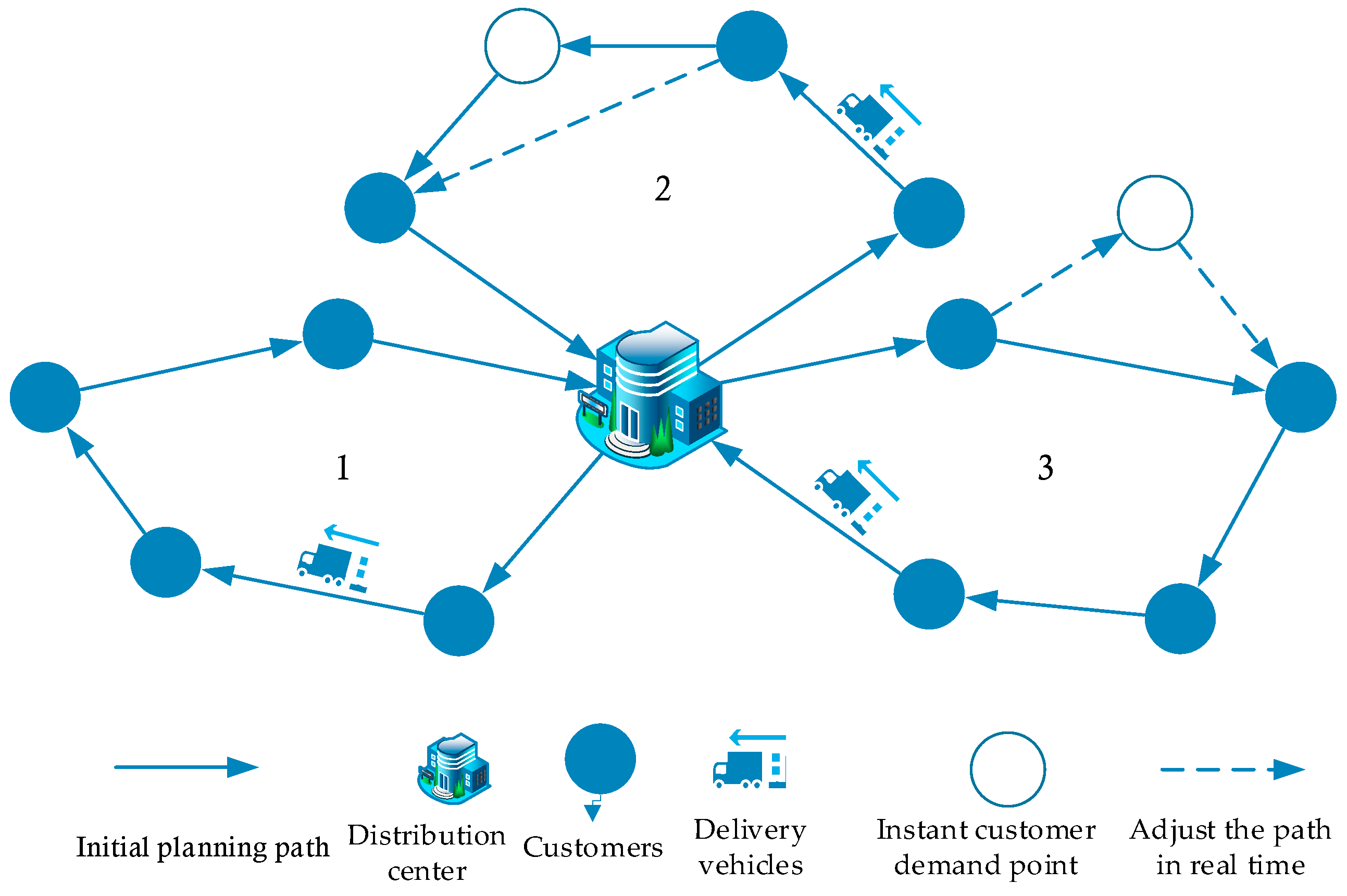
2.1. Problem Description
2.2. Distribution Cost Function
- (1)
- Vehicle fixed cost
- (2)
- Vehicle Transportation Costs
- (3)
- Temperature cost
- (4)
- Cost of carbon emissions
- (5)
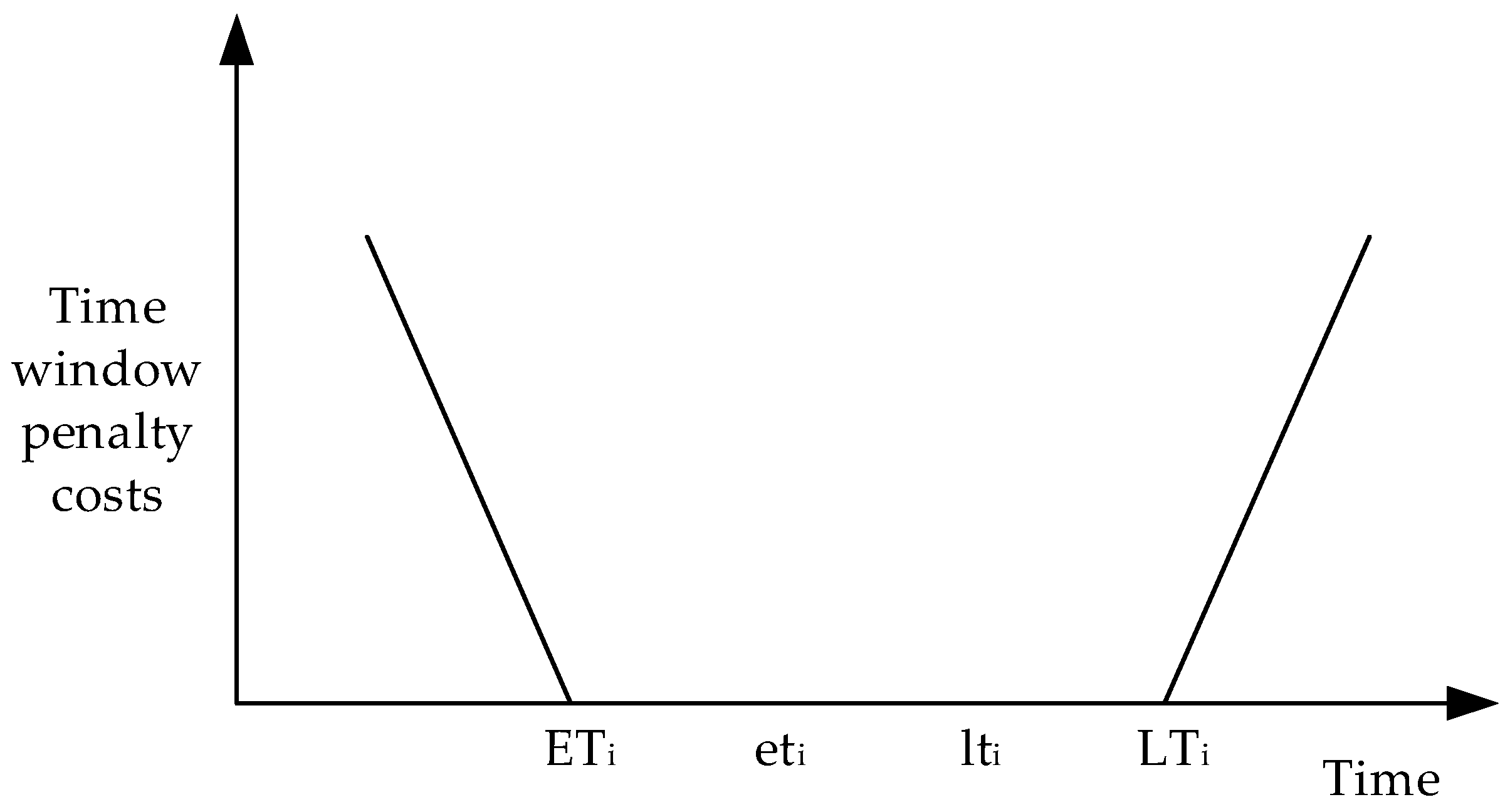
- Time window penalty cost
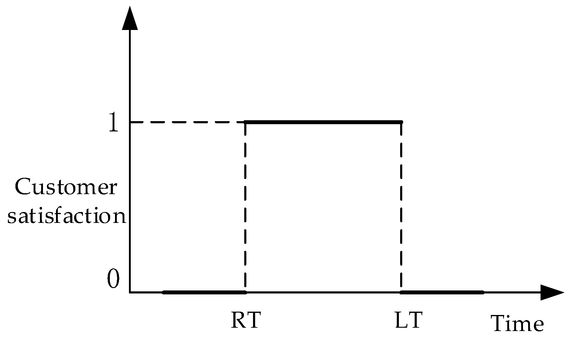
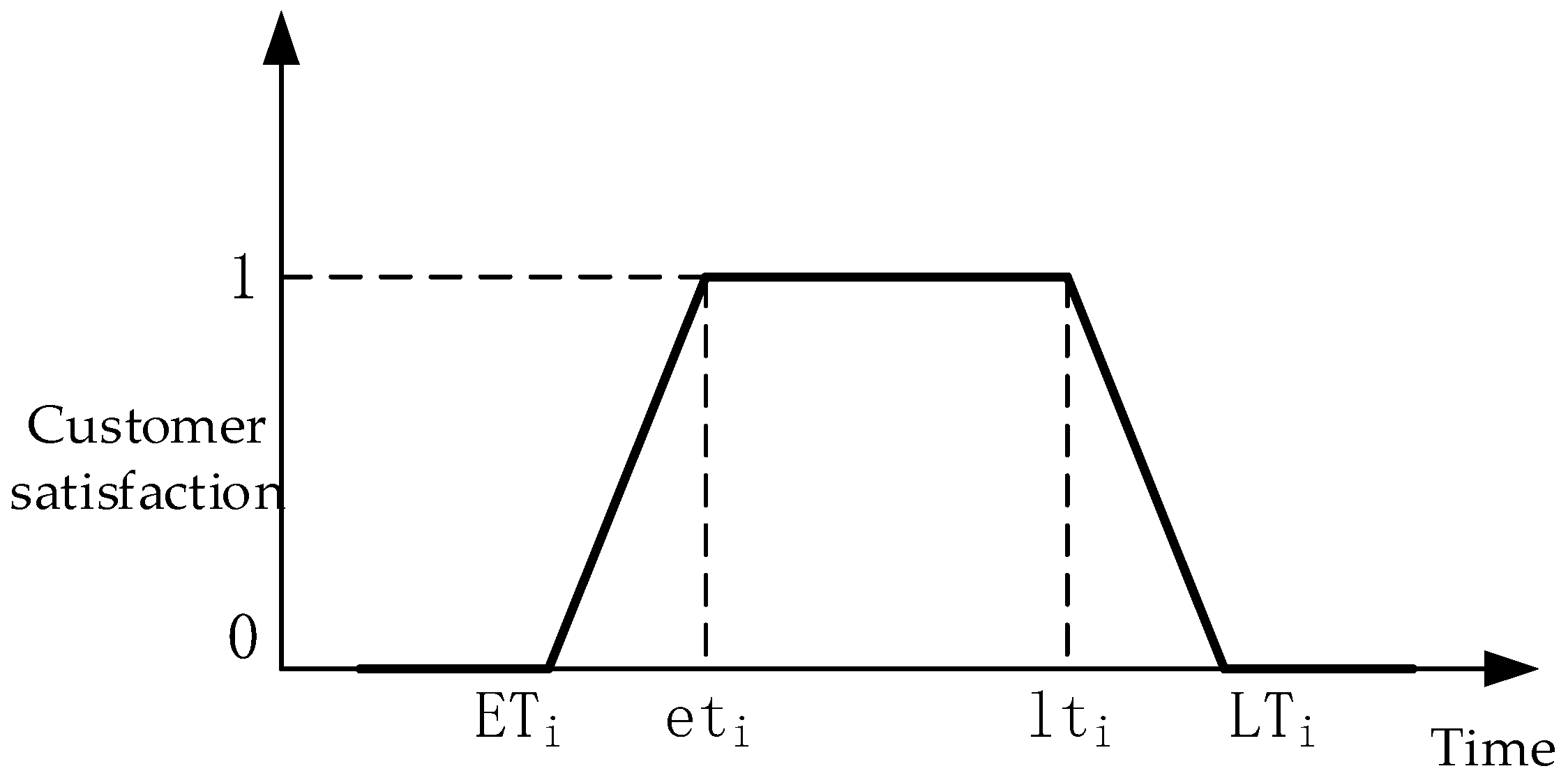
2.3. Customer Satisfaction Function
2.4. Mathematical Models
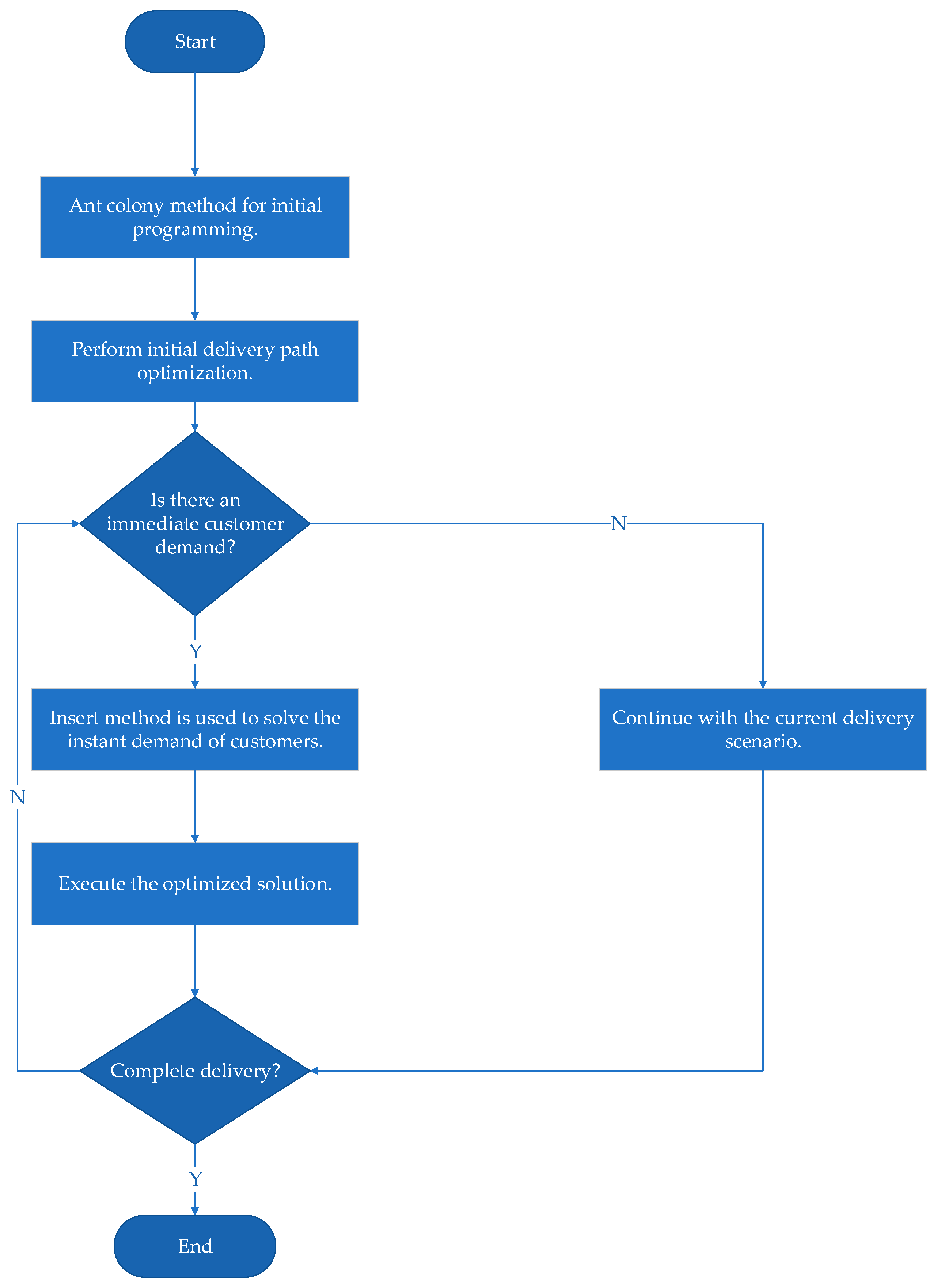
3. Algorithm Design
3.1. Algorithm for Initial Distribution Path Planning
3.1.1. Principle of Ant Colony Algorithm
3.1.2. Improved Ant Colony Algorithm
- (1)
- Adopt a saving matrix to guide the ant search
- (2)
- Improvement of the heuristic function
- (3)
- Improvement of pheromone
- (4)
- Multi-strategy improvementThis paper uses a multi-strategy approach to adjust the solutions obtained from each iteration. Moreover, we add a sequential exchange strategy [25], 2-OPT algorithm [26], and a sequential insertion strategy to the ant colony algorithm [27], in which each strategy is a neighborhood to avoid local optima to enhance the ergodicity of the ant colony algorithm search.
- (1)
- Sequential exchange strategy: Each customer point is passed through in sequence, and a customer point within the current line is exchanged with a customer on the same line or another line for the location.
- (2)
- The 2-OPT algorithm: Two points on the route are randomly selected, and the order of the remaining points remains the same, only the points between them are flipped in reverse order, which belongs to a local search algorithm.
- (3)
- Sequential insertion strategy: Insert customer points in different routes.
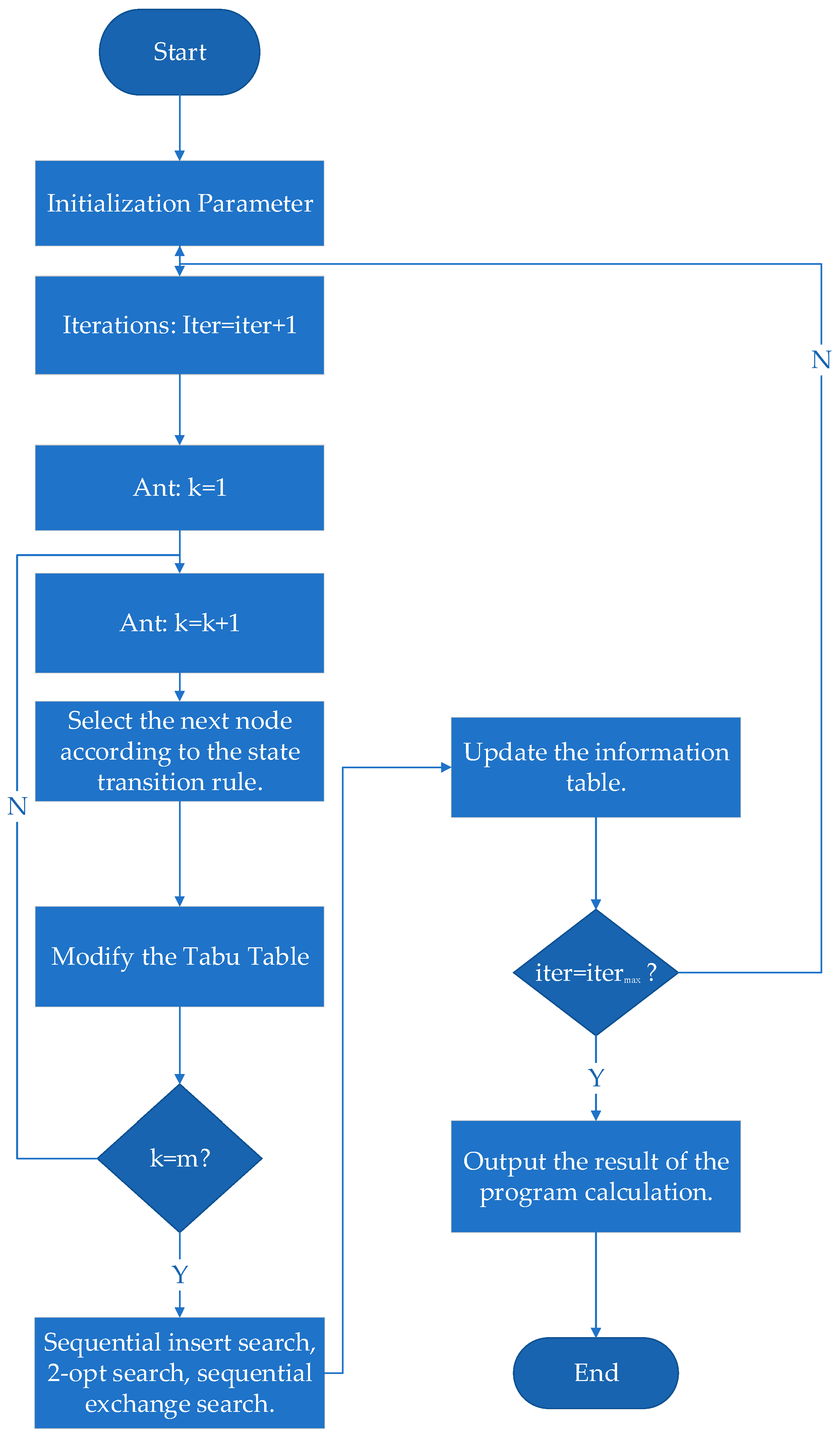
3.1.3. Improved Ant Colony Algorithm Flow
- (1)
- Initialization parameters. Let time , iteration number , set maximum iteration number , input specific data such as the distribution center and customer geographic location, set the distribution center node as the starting point of the ant, and enable chaos initialization.
- (2)
- Under the restriction of satisfying multiple constraints, each ant selects the next node according to Equation (26), records it in the forbidden table, and updates the load information of the vehicle.
- (3)
- Determine whether all ants visit all customer points. If not, repeat the step; if yes, put all customer points into the forbidden table and return to the logistics distribution center.
- (4)
- Multi-strategy improvement is performed.
- (5)
- Update the pheromone using the pheromone update rule Formula (29) of chaotic perturbation.
- (6)
- When the number of loops reaches the set maximum number of loops, the algorithm is terminated, and the optimal result of the algorithm is output. Conversely, the taboo table is emptied, and a new round of loops is started, .
- (7)
- Output the calculation results.
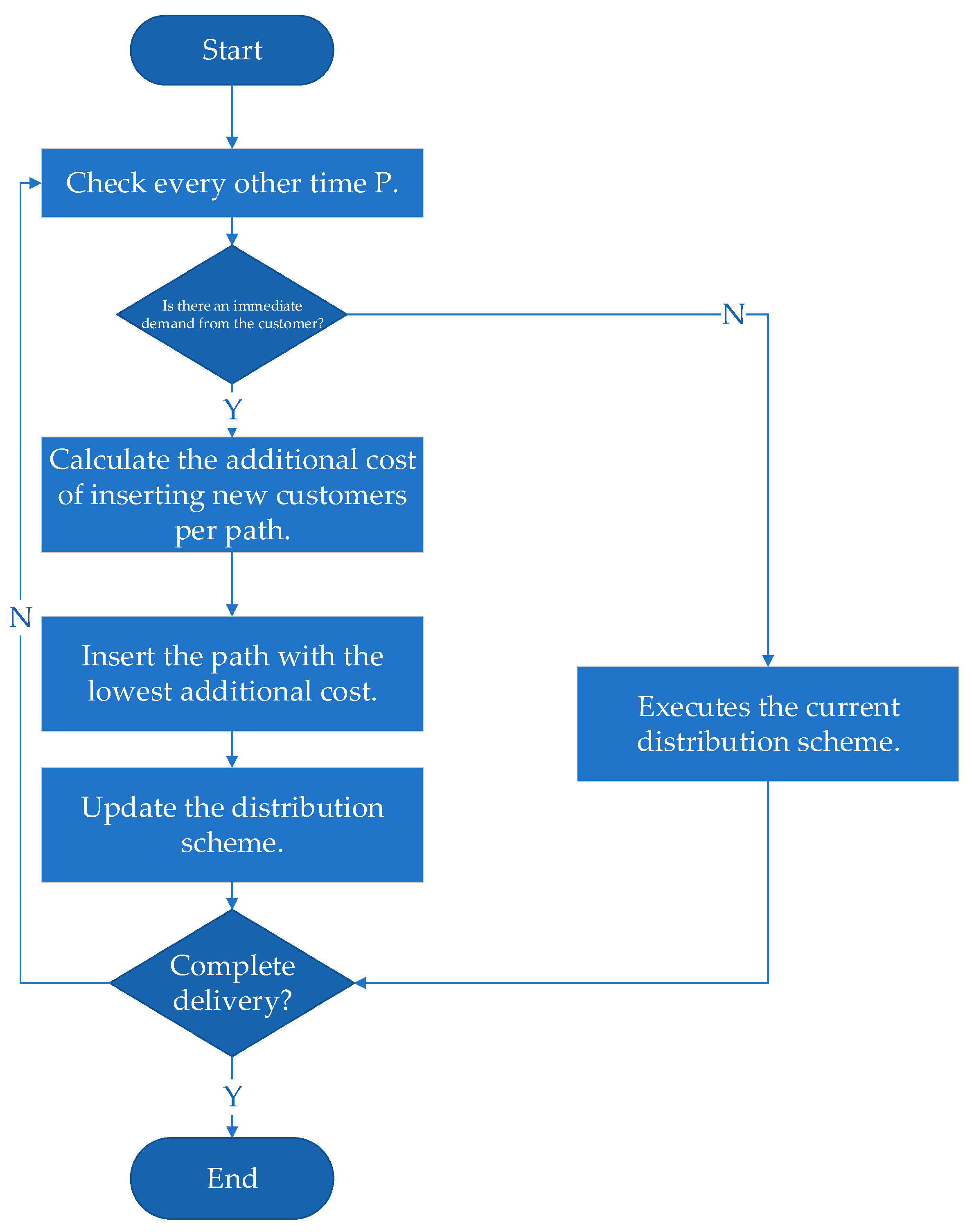
3.2. Delivery Path Algorithm for Immediate Customer Demand Phase
4. Example Analysis of the Calculation
4.1. Background Analysis and Parameter Setting
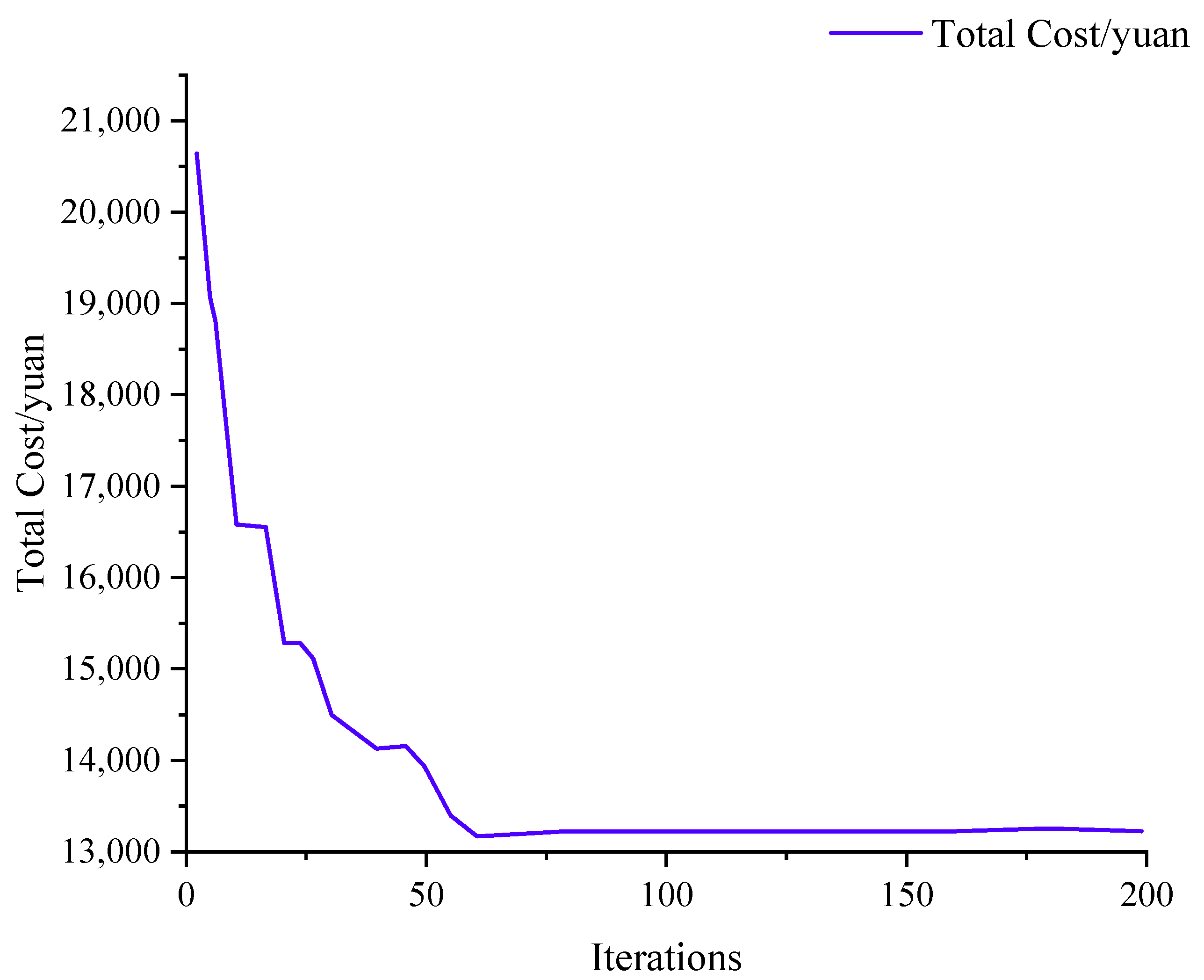
4.2. Analysis of Results
- (1)
- Solving under the initial distribution demand
- (2)
- Problem solving under immediate customer demand
5. Conclusions
Author Contributions
Funding
Institutional Review Board Statement
Informed Consent Statement
Data Availability Statement
Acknowledgments
Conflicts of Interest
References
- Sangka, B.K.; Rahman, S.; Yadlapalli, A.; Jie, F. Managerial competencies of 3pl providers. Int. J. Logist. Manag. 2019, 30, 1054–1077. [Google Scholar] [CrossRef]
- Luo, W.; Sandanayake, M.; Zhang, G.; Tan, Y. Construction cost and carbon emission assessment of a highway construction—A case towards sustainable transportation. Sustainability 2021, 13, 7854. [Google Scholar] [CrossRef]
- Xu, P.; Zhu, J.; Li, H.; Xiong, Z.; Xu, X. Coupling analysis between cost and carbon emission of bamboo building materials: A perspective of supply chain. Energy Build. 2023, 280, 112718. [Google Scholar] [CrossRef]
- Qi, Y.; Harrod, S.; Psaraftis, H.N.; Lang, M. Transport service selection and routing with carbon emissions and inventory costs consideration in the context of the belt and road initiative. Transp. Res. Part E Logist. Transp. Rev. 2022, 159, 102630. [Google Scholar] [CrossRef]
- Xu, X.; Niu, D.; Peng, L.; Zheng, S.; Qiu, J. Hierarchical multi-objective optimal planning model of active distribution network considering distributed generation and demand-side response. Sustain. Energy Technol. Assess. 2022, 53, 102438. [Google Scholar] [CrossRef]
- Yenipazarli, A. Managing new and remanufactured products to mitigate environmental damage under emissions regulation. Eur. J. Oper. Res. 2016, 249, 117–130. [Google Scholar] [CrossRef]
- Dou, G.; Cao, K. A joint analysis of environmental and economic performances of closed-loop supply chains under carbon tax regulation. Comput. Ind. Eng. 2020, 146, 106624. [Google Scholar] [CrossRef]
- Dou, G.; Guo, H.; Zhang, Q.; Li, X. A two-period carbon tax regulation for manufacturing and remanufacturing production planning. Comput. Ind. Eng. 2019, 128, 502–513. [Google Scholar] [CrossRef]
- Wang, W.; Wang, Y.; Zhang, X.; Zhang, D. Effects of government subsidies on production and emissions reduction decisions under carbon tax regulation and consumer low-carbon awareness. Int. J. Environ. Res. Public Health 2021, 18, 10959. [Google Scholar] [CrossRef]
- Tiwari, S.; Wee, H.M.; Zhou, Y.; Tjoeng, L. Freight consolidation and containerization strategy under business as usual scenario & carbon tax regulation. J. Clean. Prod. 2021, 279, 123270. [Google Scholar] [CrossRef]
- Feng, H.; Zeng, Y.; Cai, X.; Qian, Q.; Zhou, Y. Altruistic profit allocation rules for joint replenishment with carbon cap-and-trade policy. Eur. J. Oper. Res. 2021, 290, 956–967. [Google Scholar] [CrossRef]
- Bruckner, B.; Hubacek, K.; Shan, Y.; Zhong, H.; Feng, K. Impacts of poverty alleviation on national and global carbon emissions. Nat. Sustain. 2022, 5, 311–320. [Google Scholar] [CrossRef]
- Liu, G.; Hu, J.; Yang, Y.; Xia, S.; Lim, M.K. Vehicle routing problem in cold chain logistics: A joint distribution model with carbon trading mechanisms. Resour. Conserv. Recycl. 2020, 156, 104715. [Google Scholar] [CrossRef]
- Wang, R.; Wen, X.; Wang, X.; Fu, Y.; Zhang, Y. Low carbon optimal operation of integrated energy system based on carbon capture technology, lca carbon emissions and ladder-type carbon trading. Appl. Energy 2022, 311, 118664. [Google Scholar] [CrossRef]
- Wu, Q.; Wang, Y. How does carbon emission price stimulate enterprises’ total factor productivity? Insights from china’s emission trading scheme pilots. Energy Econ. 2022, 109, 105990. [Google Scholar] [CrossRef]
- Liu, M.; Shan, Y.; Li, Y. Study on the effect of carbon trading regulation on green innovation and heterogeneity analysis from china. Energy Policy 2022, 171, 113290. [Google Scholar] [CrossRef]
- Zhang, W.; Li, G.; Guo, F. Does carbon emissions trading promote green technology innovation in china? Appl. Energy 2022, 315, 119012. [Google Scholar] [CrossRef]
- Santibanez-Borda, E.; Korre, A.; Nie, Z.; Durucan, S. A multi-objective optimisation model to reduce greenhouse gas emissions and costs in offshore natural gas upstream chains. J. Clean. Prod. 2021, 297, 126625. [Google Scholar] [CrossRef]
- Demir, E.; Hrušovský, M.; Jammernegg, W.; Van Woensel, T. Green intermodal freight transportation: Bi-objective modelling and analysis. Int. J. Prod. Res. 2019, 57, 6162–6180. [Google Scholar] [CrossRef] [Green Version]
- Jiang, M.; An, H.; Gao, X. Adjusting the global industrial structure for minimizing global carbon emissions: A network-based multi-objective optimization approach. Sci. Total Environ. 2022, 829, 154653. [Google Scholar] [CrossRef]
- Sarkar, B.; Omair, M.; Choi, S.-B. A multi-objective optimization of energy, economic, and carbon emission in a production model under sustainable supply chain management. Appl. Sci. 2018, 8, 1744. [Google Scholar] [CrossRef] [Green Version]
- Dorigo, M.; Maniezzo, V.; Colorni, A. Ant system: Optimization by a colony of cooperating agents. IEEE Trans. Syst. Man Cybern. Part B 1996, 26, 29–41. [Google Scholar] [CrossRef] [PubMed] [Green Version]
- Li, M.; Sun, X. Path optimization of low-carbon container multimodal transport under uncertain conditions. Sustainability 2022, 14, 14098. [Google Scholar] [CrossRef]
- Mejjaouli, S.; Babiceanu, R.F. Cold supply chain logistics: System optimization for real-time rerouting transportation solutions. Comput. Ind. 2018, 95, 68–80. [Google Scholar] [CrossRef]
- Wang, C.; Li, Z.; Outbib, R.; Dou, M.; Zhao, D. A novel long short-term memory networks-based data-driven prognostic strategy for proton exchange membrane fuel cells. Int. J. Hydrogen Energy 2022, 47, 10395–10408. [Google Scholar] [CrossRef]
- Englert, M.; Röglin, H.; Vöcking, B. Worst case and probabilistic analysis of the 2-opt algorithm for the tsp. Algorithmica 2014, 68, 190–264. [Google Scholar] [CrossRef] [Green Version]
- Reimann, M.; Ulrich, H. Comparing backhauling strategies in vehicle routing using ant colony optimization. Cent. Eur. J. Oper. Res. 2006, 14, 105–123. [Google Scholar] [CrossRef]
- Deng, W.; Xu, J.; Zhao, H. An improved ant colony optimization algorithm based on hybrid strategies for scheduling problem. IEEE Access 2019, 7, 20281–20292. [Google Scholar] [CrossRef]
- Zhu, A.; Wen, Y. Green logistics location-routing optimization solution based on improved ga a1gorithm considering low-carbon and environmental protection. J. Math. 2021, 2021, 6101194. [Google Scholar] [CrossRef]
- Erdmann, M.; Dandl, F.; Bogenberger, K. Combining immediate customer responses and car-passenger reassignments in on-demand mobility services. Transp. Res. Part C-Emerg. Technol. 2021, 126, 103104. [Google Scholar] [CrossRef]
- Kragh, H.; Ellegaard, C.; Andersen, P.H. Managing customer attractiveness: How low-leverage customers mobilize critical supplier resources. J. Purch. Supply Manag. 2022, 28, 100742. [Google Scholar] [CrossRef]
- Wang, S.Y.; Tao, F.M.; Shi, Y.H. Optimization of location-routing problem for cold chain logistics considering carbon footprint. Int. J. Environ. Res. Public Health 2018, 15, 86. [Google Scholar] [CrossRef] [PubMed] [Green Version]
- Shi, Y.H.; Lin, Y.; Lim, M.K.; Tseng, M.L.; Tan, C.L.; Li, Y. An intelligent green scheduling system for sustainable cold chain logistics. Expert Syst. Appl. 2022, 209, 118378. [Google Scholar] [CrossRef]
- Ren, Q.-S.; Fang, K.; Yang, X.-T.; Han, J.-W. Ensuring the quality of meat in cold chain logistics: A comprehensive review. Trends Food Sci. Technol. 2022, 119, 133–151. [Google Scholar] [CrossRef]
- Han, J.-W.; Zuo, M.; Zhu, W.-Y.; Zuo, J.-H.; Lü, E.-L.; Yang, X.-T. A comprehensive review of cold chain logistics for fresh agricultural products: Current status, challenges, and future trends. Trends Food Sci. Technol. 2021, 109, 536–551. [Google Scholar] [CrossRef]
- Rong, Y.; Yu, L.; Niu, W.; Liu, Y.; Senapati, T.; Mishra, A.R. Marcos approach based upon cubic fermatean fuzzy set and its application in evaluation and selecting cold chain logistics distribution center. Eng. Appl. Artif. Intell. 2022, 116, 105401. [Google Scholar] [CrossRef]
- Bai, Q.; Yin, X.; Lim, M.K.; Dong, C. Low-carbon vrp for cold chain logistics considering real-time traffic conditions in the road network. Ind. Manag. Data Syst. 2022, 122, 521–543. [Google Scholar] [CrossRef]
- Liu, L.; Zhang, X.; Xu, X.; Lin, X.; Zhao, Y.; Zou, L.; Wu, Y.; Zheng, H. Development of low-temperature eutectic phase change material with expanded graphite for vaccine cold chain logistics. Renew. Energy 2021, 179, 2348–2358. [Google Scholar] [CrossRef]
- Navrotskaya, A.; Aleksandrova, D.; Chekini, M.; Yakavets, I.; Kheiri, S.; Krivoshapkina, E.; Kumacheva, E. Nanostructured temperature indicator for cold chain logistics. ACS Nano 2022, 16, 8641–8650. [Google Scholar] [CrossRef]
- Meng, B.; Zhang, X.; Hua, W.; Liu, L.; Ma, K. Development and application of phase change material in fresh e-commerce cold chain logistics: A review. J. Energy Storage 2022, 55, 105373. [Google Scholar] [CrossRef]
- Tang, J.; Zou, Y.; Xie, R.; Tu, B.; Liu, G. Compact supervisory system for cold chain logistics. Food Control 2021, 126, 108025. [Google Scholar] [CrossRef]
- Lim, M.K.; Li, Y.; Song, X. Exploring customer satisfaction in cold chain logistics using a text mining approach. Ind. Manag. Data Syst. 2021, 121, 2426–2449. [Google Scholar] [CrossRef]
- Nguyen, N.-A.-T.; Wang, C.-N.; Dang, L.-T.-H.; Dang, L.-T.-T.; Dang, T.-T. Selection of cold chain logistics service providers based on a grey ahp and grey copras framework: A case study in vietnam. Axioms 2022, 11, 154. [Google Scholar] [CrossRef]
- Liu, K.; He, Z.; Lin, P.; Zhao, X.; Chen, Q.; Su, H.; Luo, Y.; Wu, H.; Sheng, X.; Chen, Y. Highly-efficient cold energy storage enabled by brine phase change material gels towards smart cold chain logistics. J. Energy Storage 2022, 52, 104828. [Google Scholar] [CrossRef]
- Li, K.; Li, D.; Wu, D. Carbon transaction-based location-routing- inventory optimization for cold chain logistics. Alex. Eng. J. 2022, 61, 7979–7986. [Google Scholar] [CrossRef]
- Sha, Y.; Hua, W.; Cao, H.; Zhang, X. Properties and encapsulation forms of phase change material and various types of cold storage box for cold chain logistics: A review. J. Energy Storage 2022, 55, 105426. [Google Scholar] [CrossRef]


| Variable Classification | Symbol | Connotation and Unit |
|---|---|---|
| Parametric variable | A collection of vehicles providing fresh produce delivery services, ; | |
| The collection of distribution points where transportation is required. and , where 0 is the distribution center, and the others are the demand points; | ||
| Fixed cost of using any of the delivery vehicles; | ||
| Transportation cost per unit distance; | ||
| The distance between client and client ; | ||
| The time it takes for the vehicle to travel from distribution point to distribution point ; | ||
| The cost factor for product cooling during distribution; | ||
| High and low temperatures in the carriage; | ||
| Length of time required for the vehicle to load and unload at the distribution point ; | ||
| The cost factor for product cooling during loading and unloading; | ||
| The existence of temperature differences between the inside and outside of the carriage; | ||
| The load limit of the vehicle; | ||
| Customer demand ; | ||
| Vehicle shipment from customer to customer ; | ||
| Unit carbon tax price; | ||
| Carbon dioxide emission factor; | ||
| The actual time the delivery vehicle arrives at the customer demand point; | ||
| Waiting cost per unit time advance service; | ||
| Penalty cost per unit of time delayed service; | ||
| Collection variable | Optimal service time for the client ; | |
| A soft time window limit for the client ; | ||
| Decision variable | ||
| Customer Number | Longitude (E) | Latitude (N) | Demand (t) | Service Time (h) | ET | et | lt | LT |
|---|---|---|---|---|---|---|---|---|
| 0 | 108.677091 | 34.266719 | - | - | - | - | - | - |
| 1 | 108.834904 | 34.298973 | 0.9 | 0.36 | 123 | 168 | 192 | 224 |
| 2 | 108.351339 | 34.457663 | 1.2 | 0.48 | 111 | 159 | 181 | 193 |
| 3 | 108.659804 | 34.335292 | 0.6 | 0.24 | 24 | 57 | 92 | 114 |
| 4 | 108.401643 | 34.201826 | 1 | 0.4 | 15 | 36 | 54 | 121 |
| 5 | 108.431812 | 34.426692 | 0.5 | 0.2 | 113 | 142 | 154 | 171 |
| 6 | 108.686791 | 34.458481 | 1 | 0.4 | 96 | 133 | 170 | 208 |
| 7 | 108.534434 | 34.336947 | 0.5 | 0.2 | 50 | 78 | 96 | 113 |
| 8 | 108.733897 | 34.315858 | 0.7 | 0.28 | 85 | 115 | 148 | 193 |
| 9 | 108.810638 | 34.422681 | 0.6 | 0.24 | 12 | 45 | 89 | 121 |
| 10 | 108.163187 | 34.358199 | 1.3 | 0.52 | 102 | 144 | 195 | 238 |
| 11 | 108.613462 | 34.124683 | 1.1 | 0.44 | 23 | 69 | 194 | 114 |
| 12 | 108.917593 | 34.157497 | 0.6 | 0.24 | 15 | 42 | 68 | 92 |
| 13 | 108.411762 | 34.306202 | 0.7 | 0.28 | 18 | 33 | 50 | 68 |
| 14 | 108.342154 | 34.367553 | 0.7 | 0.28 | 103 | 136 | 158 | 169 |
| 15 | 108.194996 | 34.259948 | 0.9 | 0.36 | 46 | 87 | 137 | 162 |
| 16 | 108.939718 | 34.202915 | 0.8 | 0.32 | 24 | 53 | 88 | 105 |
| 17 | 108.833701 | 34.251392 | 0.6 | 0.24 | 124 | 149 | 183 | 207 |
| 18 | 108.977323 | 34.398478 | 0.8 | 0.32 | 117 | 132 | 156 | 172 |
| 19 | 108.601433 | 34.395234 | 0.7 | 0.28 | 52 | 78 | 95 | 112 |
| 20 | 108.957505 | 34.346586 | 0.5 | 0.2 | 21 | 45 | 92 | 135 |
| 21 | 108.453489 | 34.154947 | 0.6 | 0.24 | 18 | 26 | 35 | 42 |
| 22 | 108.904797 | 34.360362 | 0.7 | 0.28 | 124 | 159 | 180 | 208 |
| 23 | 108.760642 | 34.507643 | 0.5 | 0.2 | 16 | 32 | 68 | 135 |
| 24 | 108.615176 | 34.532539 | 0.7 | 0.28 | 45 | 87 | 106 | 182 |
| 25 | 109.021785 | 34.273477 | 0.7 | 0.28 | 42 | 93 | 149 | 181 |
| 26 | 108.339864 | 34.218985 | 1.3 | 0.52 | 18 | 25 | 47 | 60 |
| 27 | 108.234023 | 34.146337 | 0.8 | 0.32 | 21 | 36 | 59 | 113 |
| 28 | 108.961859 | 34.267609 | 0.6 | 0.24 | 58 | 97 | 142 | 173 |
| 29 | 108.023154 | 34.131234 | 0.7 | 0.28 | 54 | 72 | 103 | 124 |
| 30 | 108.580261 | 34.458556 | 0.5 | 0.2 | 58 | 94 | 139 | 192 |
| 31 | 108.726415 | 34.356136 | 1.1 | 0.44 | 21 | 32 | 48 | 64 |
| 32 | 108.281024 | 34.328557 | 0.6 | 0.24 | 23 | 42 | 61 | 83 |
| 33 | 108.079304 | 34.282961 | 1.1 | 0.44 | 26 | 47 | 68 | 107 |
| 34 | 108.904597 | 34.446687 | 0.7 | 0.28 | 48 | 98 | 148 | 174 |
| 35 | 109.010218 | 34.444346 | 1.2 | 0.48 | 26 | 63 | 91 | 142 |
| 36 | 108.077109 | 34.246373 | 0.5 | 0.2 | 169 | 184 | 207 | 256 |
| 37 | 108.136842 | 34.526286 | 0.7 | 0.28 | 108 | 121 | 147 | 163 |
| 38 | 108.885776 | 34.523326 | 0.6 | 0.24 | 21 | 68 | 91 | 115 |
| 39 | 109.010997 | 34.185556 | 0.7 | 0.28 | 18 | 25 | 59 | 96 |
| 40 | 109.056321 | 34.246891 | 1 | 0.4 | 76 | 98 | 135 | 164 |
| 41 | 109.137439 | 34.356827 | 0.6 | 0.24 | 23 | 48 | 89 | 154 |
| 42 | 108.718379 | 34.126482 | 0.8 | 0.32 | 113 | 143 | 165 | 201 |
| 43 | 108.107532 | 34.415861 | 0.9 | 0.36 | 91 | 105 | 134 | 148 |
| Immediate Demand Type | Customer Number | Receiving Moment | Longitude (E) | Latitude (N) | Demand (t) | Service Time (h) | ET | et | lt | LT |
|---|---|---|---|---|---|---|---|---|---|---|
| 0 | 44 | 3:54 | 108.613742 | 34.426692 | 0.8 | 0.32 | 84 | 125 | 153 | 201 |
| 0 | 45 | 4:12 | 108.709566 | 34.245249 | 0.6 | 0.24 | 149 | 172 | 196 | 256 |
| 1 | 22 | 5:13 | 108.904797 | 34.360362 | 0.7 | 0.28 | 35 | 35 | 50 | 50 |
| 1 | 18 | 5:18 | 108.977323 | 34.398478 | 0.8 | 0.32 | 137 | 137 | 148 | 148 |
| Vehicle | Route | Vehicle Load (t) | Vehicle Full Load Ratio |
|---|---|---|---|
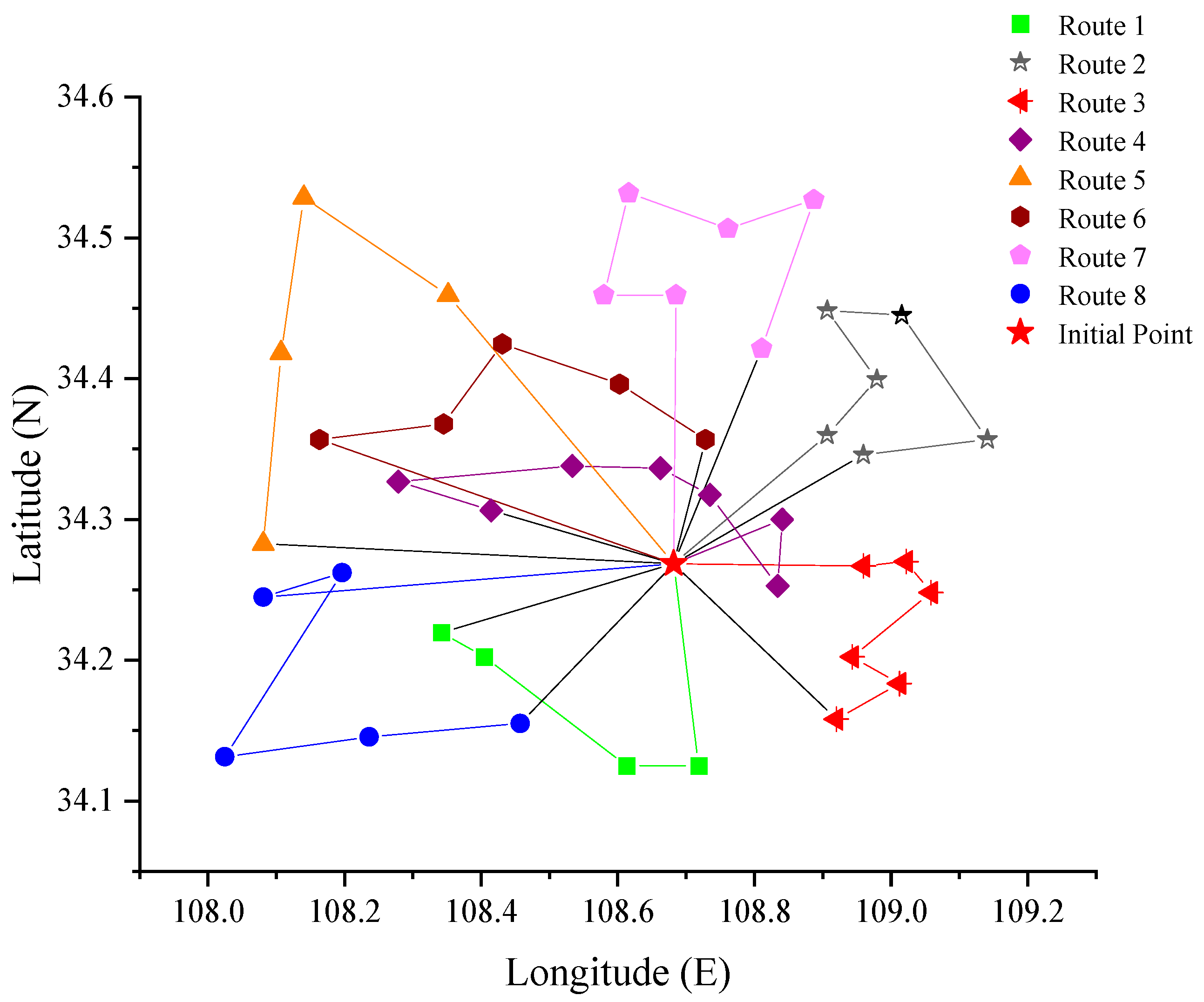
| 1 | 0-26-4-11-42-0 | 4.2 | 84% |
| 2 | 0-20-41-35-34-18-22-0 | 4.5 | 90% |
| 3 | 0-12-39-16-40-25-28-0 | 4.4 | 88% |
| 4 | 0-13-32-7-3-8-17-1-0 | 4.6 | 92% |
| 5 | 0-33-43-37-2-0 | 3.9 | 78% |
| 6 | 0-31-19-5-14-10-0 | 4.3 | 86% |
| 7 | 0-9-38-23-24-30-6-0 | 3.9 | 78% |
| 8 | 0-21-27-29-15-36-0 | 3.5 | 70% |
| Vehicles | Vehicle Fixed Costs | Vehicle Transportation Costs | Temperature Costs | Carbon Costs | Time Window Penalty Costs | Total Customer | Dissatisfaction |
|---|---|---|---|---|---|---|---|
| 1 | 350 | 685.36 | 139.98 | 184.66 | 58.5 | 1417.49 | 24.54% |
| 2 | 350 | 871.60 | 158.95 | 259.58 | 0 | 1640.14 | 12.26% |
| 3 | 350 | 689.12 | 143.53 | 187.99 | 0 | 1370.64 | 16.86% |
| 4 | 350 | 887.68 | 162.25 | 284.09 | 166.5 | 1850.52 | 22.10% |
| 5 | 350 | 1123.57 | 164.61 | 283.91 | 0 | 1922.09 | 15.29% |
| 6 | 350 | 916.35 | 157.98 | 160.03 | 0 | 1584.36 | 19.44% |
| 7 | 350 | 797.08 | 140.80 | 195.84 | 0 | 1483.72 | 13.69% |
| 8 | 350 | 1210.74 | 162.48 | 208.09 | 91 | 2022.32 | 24.87% |
| Immediate Demand Type | Customer Number | Receiving Moment | Vehicle | Distribution Cost (yuan) | Adjusted Distribution Path |
|---|---|---|---|---|---|
| 0 | 44 | 3:54 | 7 | 1576.46 | 0-9-38-23-24-30-44-6-0 |
| 0 | 45 | 4:12 | 1 | 1472.39 | 0-26-4-11-42-45-0 |
| 1 | 22 | 5:13 | 2 | 1897.15 | 0-20-22-41-35-18-34-0 |
| 1 | 18 | 5:18 | 2 | 1897.15 | 0-20-22-41-35-18-34-0 |
| Vehicle 1 | Vehicle 2 | Vehicle 3 | Vehicle 4 | Vehicle 5 | Vehicle 6 | Vehicle 7 | Vehicle 8 | |
|---|---|---|---|---|---|---|---|---|
| Total load rate of distribution vehicles under initial demand | 84% | 90% | 88% | 92% | 78% | 86% | 78% | 70% |
| Total load rate of delivery vehicles under immediate customer demand | 96% | 90% | 88% | 92% | 78% | 86% | 94% | 70% |
Disclaimer/Publisher’s Note: The statements, opinions and data contained in all publications are solely those of the individual author(s) and contributor(s) and not of MDPI and/or the editor(s). MDPI and/or the editor(s) disclaim responsibility for any injury to people or property resulting from any ideas, methods, instructions or products referred to in the content. |
© 2023 by the authors. Licensee MDPI, Basel, Switzerland. This article is an open access article distributed under the terms and conditions of the Creative Commons Attribution (CC BY) license (https://creativecommons.org/licenses/by/4.0/).
Share and Cite
Ma, Z.; Zhang, J.; Wang, H.; Gao, S. Optimization of Sustainable Bi-Objective Cold-Chain Logistics Route Considering Carbon Emissions and Customers’ Immediate Demands in China. Sustainability 2023, 15, 5946. https://doi.org/10.3390/su15075946
Ma Z, Zhang J, Wang H, Gao S. Optimization of Sustainable Bi-Objective Cold-Chain Logistics Route Considering Carbon Emissions and Customers’ Immediate Demands in China. Sustainability. 2023; 15(7):5946. https://doi.org/10.3390/su15075946
Chicago/Turabian StyleMa, Zhichao, Jie Zhang, Huanhuan Wang, and Shaochan Gao. 2023. "Optimization of Sustainable Bi-Objective Cold-Chain Logistics Route Considering Carbon Emissions and Customers’ Immediate Demands in China" Sustainability 15, no. 7: 5946. https://doi.org/10.3390/su15075946