A Study of CNN and Transfer Learning in Medical Imaging: Advantages, Challenges, Future Scope

Abstract

This paper presents a comprehensive study of Convolutional Neural Networks (CNN) and transfer learning in the context of medical imaging. Medical imaging plays a critical role in the diagnosis and treatment of diseases, and CNN-based models have demonstrated significant improvements in image analysis and classification tasks. Transfer learning, which involves reusing pre-trained CNN models, has also shown promise in addressing challenges related to small datasets and limited computational resources. This paper reviews the advantages of CNN and transfer learning in medical imaging, including improved accuracy, reduced time and resource requirements, and the ability to address class imbalances. It also discusses challenges, such as the need for large and diverse datasets, and the limited interpretability of deep learning models. What factors contribute to the success of these networks? How are they fashioned, exactly? What motivated them to build the structures that they did? Finally, the paper presents current and future research directions and opportunities, including the development of specialized architectures and the exploration of new modalities and applications for medical imaging using CNN and transfer learning techniques. Overall, the paper highlights the significant potential of CNN and transfer learning in the field of medical imaging, while also acknowledging the need for continued research and development to overcome existing challenges and limitations.

1. Introduction

People’s health is at the center of medical care. The amount of medical data available today is enormous, but to benefit the medical industry [1], it is essential to use this data wisely. Medical images are frequently requested in accordance with a patient’s follow-up to ensure that therapy was successful, and it is a critical step in the process of medical diagnosis and treatment [2]. In general, a radiologist examines the obtained medical images and compiles their results in a report [3]. Based on the images and the reports from radiologists, the referring doctor determines a diagnosis and a course of action. The majority of medical professionals, particularly radiologists, interpret medical images. However, human subjectivity, the wide variances among interpreters, and weariness limit human image interpretation. Due to the limited time radiologists have to analyze an ever-growing number of images, missed findings, lengthy turnaround times, and a lack of quantitative data or quantification are common when reviewing cases [4,5]. In turn, this severely restricts the medical profession’s potential to expand the use of evidence-based, individualized healthcare [6]. Artificial Intelligence (AI) is a broad field with a wide variety of subfields such as natural language processing (NPL) [7], speech processing [8], machine learning, deep learning, robotics, etc. [9]. AI is applied in various kinds of fields, such as healthcare, agriculture, manufacturing, and the education sector [10]. Machine learning is a branch of AI that can learn from the data itself, automatically identify the patterns in data, and make decisions with minimum human intervention [11,12]. Over recent years, deep learning techniques have gained a lot of attention to solve various problems, especially in medical imaging fields [13]. Deep learning is an advanced field in computer vision. The purpose of computer vision is to carry out multiple tasks such as image detection, image recognition, NPL, image analysis [14], etc. A CNN is a type of artificial neural network specially designed to handle video and image data. It takes input images, extracts them, and classifies the output images after learning the features from the input images based on the learning features [11]. The deep learning CNN technique is used in the majority of AI medical image analyses, especially for the diagnosis of different types of diseases [15] such as breast cancer, Alzheimer’s, brain tumors [16], etc. [4,17]. Deep CNN-based algorithms have achieved promising outcomes in the analysis of medical images. Several types of TL have been proposed for medical imaging data and have been very effective, such as Alex Net, SPP-Net, VGGNet, ResNet, GoogLeNet, etc. [4]. The major aim of this review is to highlight the most crucial CNN components so that researchers and students may easily gain a comprehensive understanding of CNN and transfer learning. This article will assist individuals to learn more about recent advancements in the discipline, which will promote DL research. The following list outlines our contributions:

• This review aids in the comprehension of CNN and transfer learning techniques among researchers and students.
• We simply describe the major issues of traditional ML and how DL-based techniques like CNN can come to the rescue and play an important role in diagnostic analysis.
• We describe in-depth the ideas, theories, and cutting-edge architectures of CNN, the most well-known deep learning technique.
• A literature review is provided in this paper to give an overview of related research work done on the use of CNN and TL techniques.
• We discuss the difficulties that deep learning-based techniques currently face, such as the scarcity of training data, overfitting, and vanishing gradient problems.
• The strategies for choosing the right TL-based technique for a problem are discussed.
• We also present a list of medical imaging modalities used in training the model, and we describe computational resources such as GPU, CPU, and TPU by contrasting how each tool affects deep learning algorithms.

CNNs’ application to medical image processing is first discussed in this paper. The difference between traditional ML and DL-based algorithms and the analysis of medical images are presented in Section 2. Then we give a detailed overview of the architecture of CNN in Section 3. The corresponding work in the field of diagnosing disease using medical images, including CT, MRI, fMRI, PET, X-ray, and ultrasound, is discussed in Section 4. We also described the significance and importance of transfer learning techniques and explain each with their potential benefits in Section 5. Finally, we discuss the possible problems and predict the development prospects of CNN-based techniques in medical imaging analysis.

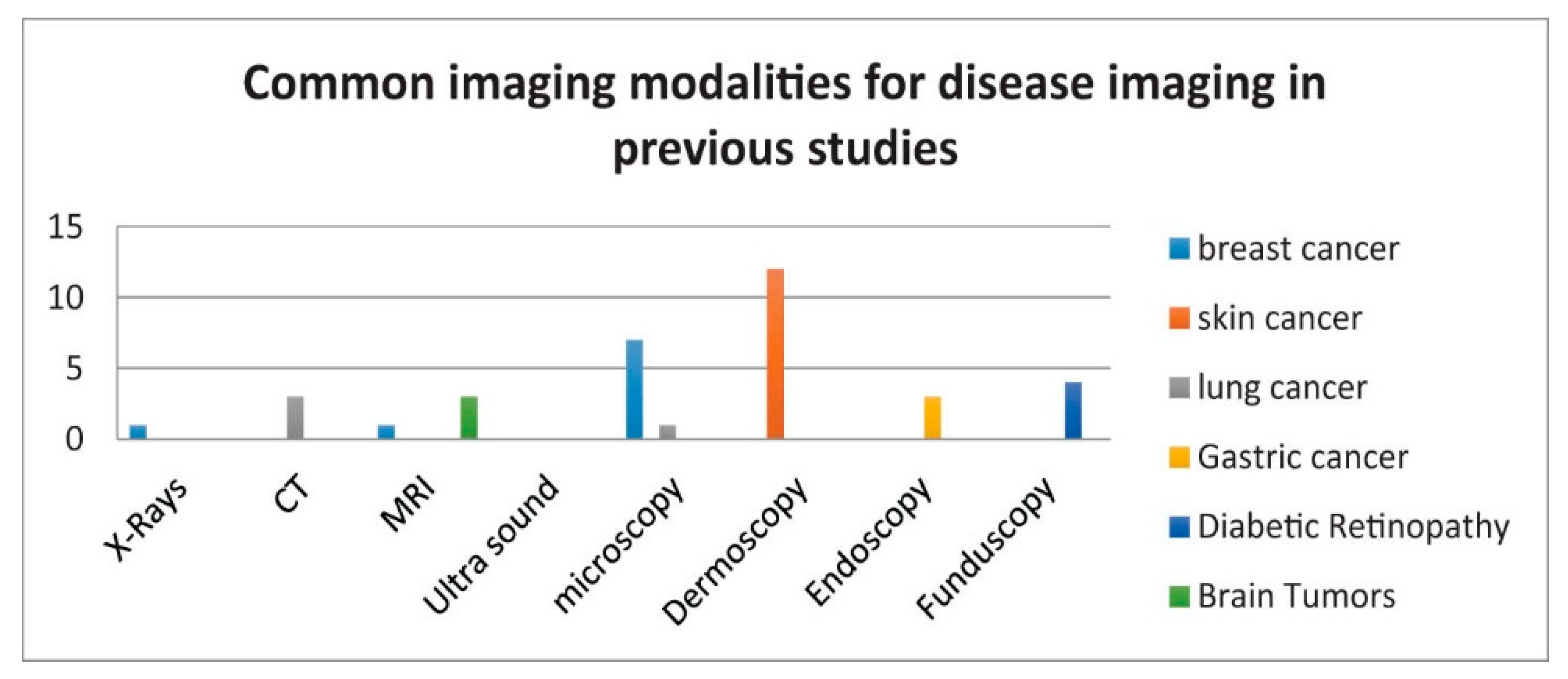
2. Imaging Modalities for Analytics and Diagnostics

To create an image, several methods are used. Examples of these measurements are radiofrequency signal capacity in an MRI, sound pressure for ultrasounds, and radiation absorption in X-ray imaging. In a digital image, one measurement is used to determine each image point, while in multi-channel images, several measurements are gathered [18]. To create diagnostic images, a wide variety of imaging modalities are employed, such as computed tomography (CT), X-ray, magnetic and functional resonance imaging (MRI and fMRI) [19], and positron emission tomography (PET) scans [4,5]. Common DL applications using medical imaging include image classification [11], segmentation, synthesis, and regression [12,20]. Figure 1 depicts various imaging modalities used [21]. In the initial phase of using more precise imaging methods to halt the spread of disease, medical imaging techniques are crucial as an aid to early diagnosis in the treatment or eradication of many medical disorders.

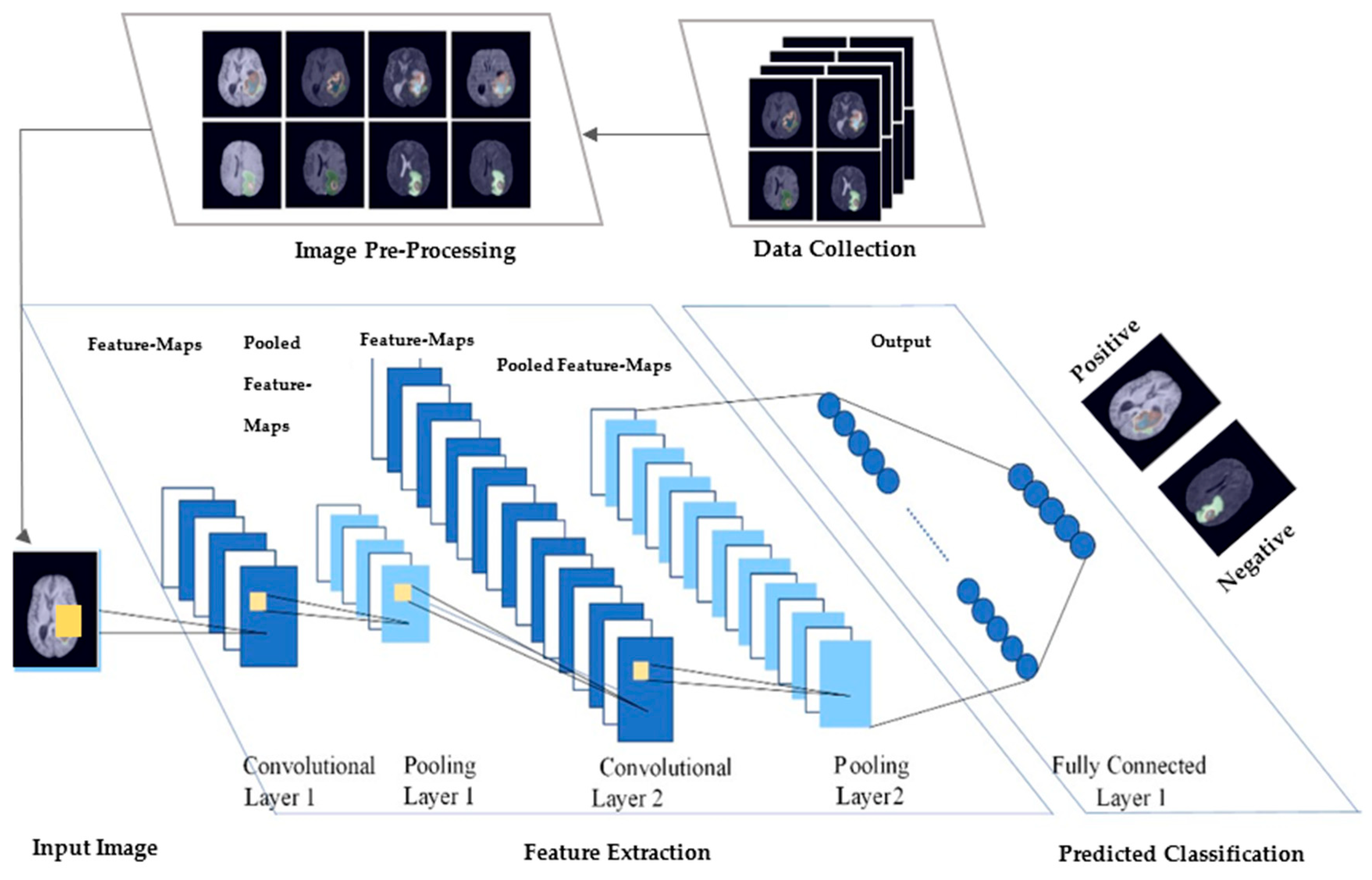
3. Convolutional Neural Network and its Background

David Hubel and Torsten Wiesel, two neurophysiologists, did experimentation in 1959 and eventually published their findings in a work titled “Receptive-Fields of Single-Neurons in cat’s straits cortex” [22]. They defined how the neurons in a cat’s brain are organized in a tiered pattern or layered form. These are the layers that can learn to detect visual patterns with the help of local features, which are extracted first, and for a higher-level representation, the extracted features are then combined [23]. Consequently, this concept is effectively becoming one of deep learning’s core principles. In 1980, another researcher by the name of Kunihiko, who was motivated by the work of T. Wiesel [22], proposed a “Neocognitron”. This work proposed a multi-layered neural network for the hierarchical detection of visual patterns learned from data (learning-without-teacher), which is known as a self-organizing neural network. [24]. This design then became the first CNN theoretical model. The Neocognitron develops the ability to classify and accurately detect patterns based on their shape distinctions. Any patterns that we humans consider to be similar are also classified as such by this proposed model. CNN, commonly known as ConvNet, is one of the common types of Artificial Neural Network (ANN) [25] that comes under the supervised method category. This method is known for its ability to discover and interpret patterns. This pattern detection brings up the usefulness of CNN for image analysis [26]. A ConvNet is a series of layers in which each layer performs some unique functions. Furthermore, these layers are usually classified into different categories [27]. The raw data is stored in the first layer, called the input layer. A convolutional layer is the second layer, which is responsible for calculating the output volume by performing a dot product between the image patch and all of the filters, followed by another important function known as activation. The mathematical function is then applied to every element of the convolution layer’s output. The next layer comes in to help in reducing the computation costs by making the previous layer’s output memory efficient. It is known as the pooling layer. Finally, once the pooling layer computation is done, it will pass its output to the last layer and output the computed 1-D array class score [26]. Two primary tasks must be accomplished when training a deep learning model:

• Forward propagation: To train a neural network, one must first provide it with an input, and then, in light of the outcomes of that processing, an output is produced.
• Backward propagation: Next, the model uses the backpropagation technique, such that the weights of the neural network are modified in response to the error that was obtained in the forward propagation.

3.1. Important Elements of CNN

In this part of the article, we discuss the fundamental components of a CNN in detail with their role in the whole architecture:

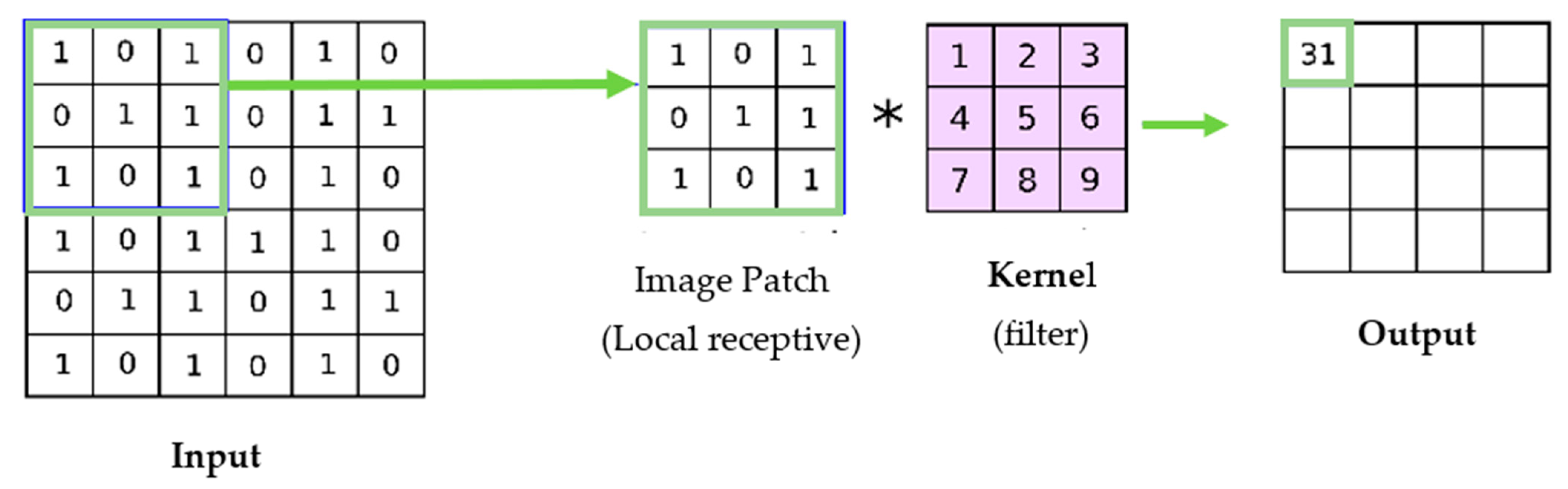
3.1.1. Convolutional Layer

The convolution layer, as its name suggests, is crucial to CNN’s operation. Where the majority of the calculation is concerned, it is the core unit of a CNN. Since digital image processing is concerned, convolution operations are the most widely used [19]. Convolutional layers are where filters (also known as the set of kernels) are applied or get convolved with the original input images, which can be n-dimensional metrics to generate a feature map as an output [20]. Here, the number of kernels and the size of the kernels are the most critical parameters, which refer to the size of the filter, as shown in below Figure 2. The following mathematical formula is used to determine subsequent feature map values [20], where the kernel is denoted by h and the image input is indicated by f. The result matrix’s row and column indexes are denoted by m and n.

$$G\left[m, n\right]=\left(fx\right)\left[m, n\right]={\displaystyle \sum }_j {\displaystyle \sum }_k h\left[j,k\right]f\left[m-j, n-k\right]$$

(1)

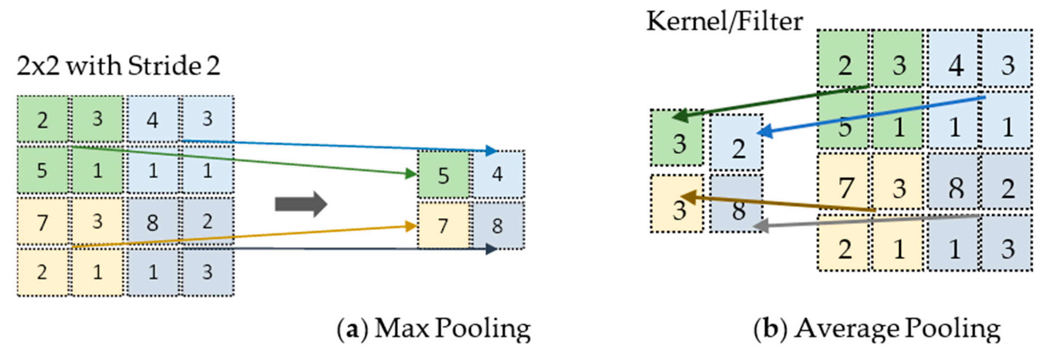
3.1.2. Pooling Layer

In CNN, the convolutional operation is applied to learned filters to the input image to summarize and show the presence of those features in the given. This is done in a systematic way to build its feature maps. The feature map is generated by the convolutional layer’s output. It has one limitation due to recording the exact location of features in the input. Therefore, in the input image, any small movement that happens to the position of a feature, such as re-cropping, rotation, etc., will cause changes in the feature map. A common solution to this problem can be achieved in the convolution layer using downsampling by altering the convolution stride over the image [28]. This is where the usage of the pooling layer begins. It is nothing but a common and robust approach to the same problem. In a short pooling layer downsample, the previous layers’ feature map and pooling operations aid in the creation of an invariant representation for small input translations [29]. Additionally, there are several functions used for specifying the pooling procedure; the most common functions are the following [30]:

(a)

Average pooling: This is used when the average value is desired for each patch on the feature map.

(b)

Maximum pooling: This is commonly known as Max-pooling, and is used when the maximum value is desired for each patch on the feature map [30]. Below Figure 3, illustrate the working of average and maximum pooling.

3.1.3. Fully Connected Layers

Immediately following the completion of feature extraction and consolidation by the convolutional and pooling layers, another layer comes in, which is known as the fully connected layer [31]. This component is connected to the final node of each network to flatten out the output of the previous layer. Finally, this layer returns the probability of class predictions by building non-linear feature combinations. There are various non-linear functions, such as activation functions, ReLU, and Softmax.

3.2. Important Parameters and Hyperparameters for Building CNN

The following are the important parameters with a high level of description.

• Kernels: The kernel is nothing but a matrix that is used to traverse over the input images to perform a dot product to extract features [32]. By using the stride value, the kernel can move by columns of pixels based on the number assigned to the stride.
• Biases: Before passing the output values through an activation function, the bias is used to adjust the scaled values. For example, in a neural network, the activation function receives an input ‘x’ which is multiplied by the ‘w’ weight. Therefore, adding a constant bias to the input will enable you to shift the activation function [33].
• Padding: When a kernel is used with image processing, the image is altered each time a convolution is carried out on the input data. The image shrinks and thus this can be done only a certain number of times before the input image completely disappears [34]. As a result, some of the information contained in the image can be lost. The problem is that when the kernel moves across the image there is a significant impact on the pixels in the outskirts of the image, which are much smaller when compared to the center pixels of the image [35]. Therefore, a more accurate analysis of the image can be achieved by the use of padding, which is added to the image’s outer frame to provide more room for the filter to cover the image.
• Stride: Stride is another so-called hyperparameter in the convolutional layer that specifies the pixel count the kernel shifts over the input image matrix. For instance, when two is set as the stride, then the filter or kernel moves two pixels at a time. When three is set as stride, then the filter moves three pixels at a time, and so on [36].
• Dropout for regularization: This is a powerful yet simple regularization technique for deep learning models [37], and CNNs usually have the habit of overfitting. When there are a large number of nodes or neurons in a full-connected layer, it is more likely that co-adaptation occurs. Co-adaption simply means when many neurons in a single layer extract very similar or the same hidden features from the given input data. This usually happens when two different neurons’ connection weights are identical [38]. This technique works based on selecting neurons randomly and ignoring them during training; they will lose their contribution for further processes.
• Learning Rate: The learning rate is a very important parameter in CNN which defines how swiftly a network updates its parameters during backpropagation [39]. Keeping the learning rate low makes the convergence smooth, but the learning process slows down. However, keeping the learning rate larger may speed up the process of learning, but may prevent convergence.

Activation Functions: Nonlinearity is introduced to models via activation functions, allowing deep-learning models to learn nonlinear prediction bounds. In artificial neural networks (ANNs), activation functions are used to transform an input signal into an output signal. This output signal is then used as input by the subsequent layer in the stack. The most common activations used in CNN are described below:

Sigmoid activation function: Because it is a non-linear function, it is the most often utilized activation function. The sigmoid function changes data in the 0 to 1 range and it is widely used for binary classification. It can be summed up as follows [40]:

$$f\left(x\right)=\frac{1}{e^{-x}}$$

Tanh activation function: It is a function known as the hyperbolic tangent. The Tanh function is comparable to the sigmoid function; however, it is symmetric concerning the origin [40]. This activation function is smoother, and it is a zero-centered function with a scale that goes from −1 to 1, therefore, the function’s output is given as [41]:

$$f\left(x\right)=\left(\frac{e^x-e^{-x}}{e^x-e^{-x}}\right)$$

In contrast to the sigmoid function, the Tanh function became the favored function because it provides higher training performance for a model with multiple layers [42,43].

ReLU function: ReLU stands for the rectified linear unit; it is a non-linear function and very popular in ConvNets. Since all the neurons are not going to be activated at the same time, but rather a small number of neurons are activated at a time, the ReLU function is more efficient than others [40]. According to equation 1, the output of ReLU is the value that is greater than either zero or the value that was fed into the model. When the value of the input is negative, the value of the output is equal to 0. When the value of the input is positive, the output value will be equal to the value of the input [44].

$$f\left(x\right)=\max \left(0,x\right)$$

An improved version of the ReLU activation function came up after ReLU, where instead of specifying the ReLU function’s value as zero for x (negative values), rather it is defined as an x having an extremely insignificant linear component. It can be mathematically stated as [40]:

$$\begin{gathered} f\left(x\right)=0.01x, x<0 \\ f\left(x\right)=x, x\ge 0 \end{gathered}$$

Softmax activation function: For binary (0, 1) classification, the sigmoid function is used, but to deal with multiclass classification Softmax is used. The Softmax function returns a probability for each data point of all individual classes [40]. Therefore, in a deep neural network, when we want to work with a multiclass classification problem, the output layer of the neural network will have an identical amount of network neurons that correspond to the number of target classes. The formula is stated as follows [13]:

$$\sigma \left(z\right)j=\frac{e^{z_j}}{{{\displaystyle \sum }}_{k=1}^K{e}^{z_j}} for j=1,\dots ..K$$

Figure 4 represents the process for these connected layers.

4. ConvNets over Traditional Machine Learning

The process of machine learning involves the use of algorithms to analyze data, draw conclusions from that analysis, and make decisions based on those conclusions. In the case of DL, it uses multiple layers to create an ANN [7]. Each layer provides different information about the data which is fed to them. To perform classification work using machine learning techniques, several preprocessing steps, such as feature selection, [46], feature extraction [47], and classification are required [48]. Even the selection of features can have a significant impact on the efficiency gains achieved through various machine-learning strategies. DL techniques can perform automated feature sets for various tasks. Deep learning has simplified the improvement of object detection, image super-resolution, image classification, and image recognition fields [49].

Typical healthcare applications of classification tasks of images include Alzheimer’s disease (AD) classification using MRI [50], dermatological identification of skin conditions [51], breast cancer diagnosis using histopathological images [17], and diagnosis of eye diseases in the field of ophthalmology (such as diabetic retinopathy [52], corneal diseases [53], and glaucoma [54]). With advances in 2021, DL has become a key popular tool for the automatic detection of COVID-19 and classifying healthy and not-healthy individuals using X-rays and CT scan images [50].

4.1. The Problem with Traditional Neural Networks

The main significant distinction between the traditional ANNs and CNNs is the primary usage of ConvNets in the field of pattern recognition, in particular of medical images. This usage enables the developers to encode features of input images into the architecture and makes the convolutional neural network more beneficial for image-specific tasks, while also lowering the number of parameters needed to set up and build the model. Traditional neural networks are known as multilayer perceptrons (MLPs). MLPs have several limitations, particularly when it comes to the processing of images [55]. For each input, MLPs are going to use a single perceptron, which means if we input an RGB image, each pixel is going to be multiplied by three since there are three channels in RGB. Therefore, here is where the problem arises; the number of weights to be used in each perceptron rapidly increases for large images, so it becomes unmanageable for the model. There are approximately 187,000 weights to train for a 250 × 250-pixel image with three channels. Hence, overfitting can happen, and training becomes difficult [56].

4.2. Feature Extraction

Feature extraction entails the process of obtaining a high level of patterns from raw pixel values to seize the uniqueness of the distinction between the various categories that are being used. The extraction of these features is carried out without the presence of any supervision (unsupervised manner). This indicates that the information that is extracted from the pixels of the image has nothing to do whatsoever with the classes of the image, and, in CNN, the convolution layer is the backbone of feature extraction [57]. This allows for the sharing of parameters. Following the extraction of the features [58], a classifier is then trained using the images and the labels that are associated with them, for example, logistic regression, random forests, decision trees, support vector machines, etc. This pipeline has a problem due to the fact that the feature extraction cannot be changed based on the classes and images. So, no matter what type of classification technique is used, the accuracy of the model is severely compromised as a result if the chosen feature does not give enough information to tell the categories apart [59]. Picking various feature extractors and clubbing them ingeniously to achieve better feature extraction has been a recurrent subject among state of the art studies. However, this necessitates an excessive number of heuristics and tedious manual work to adjust settings depending on the domain. The main philosophy behind deep learning is that there is no predetermined way to extract features (no hard-coding) from data [60]. The CNN learns to extract data by differentiating representations from the input images and to categorize them based on supervised data, all inside a single integrated system.

4.3. Parameter Sharing

With ConvNets, a large dataset like ImageNet can be used to train the whole network from scratch [61]. ImageNet is an ongoing project that has so far collected 14,197,122 images in 21,841 different categories. Sharing parameters cuts down on the total parameters in the network and shortens the training time required for the network [59].

5. Literature Review

For the last few years, researchers have been using CNN-based models to extract unique and useful features for the diagnosis of various diseases, including but not limited to brain cancer, heart disease, Alzheimer’s disease (AD), COVID-19, Parkinson’s disease, breast cancer, etc. [62], by using medical images. According to previous studies, using convolutional neural network-based models achieved a good level of accuracy when compared with traditional machine learning and volumetric techniques that are manually performed by physicians. Therefore, this section summarized the CNN-based methods using medical images.

In the Alexander et al. [63] study, a CNN model using MRI and diffusion-tensor imaging (DIO) was used for the classification of AD patients. According to their study, the classification performance demonstrates that the size of the hippocampal region of interest (ROI) does not matter when bigger ROIs are combined with using CNN architecture for the classification. Using a six-layered convolutional neural network with 48 × 48 × 48 ROI with a data fusion model achieved a good accuracy of 96.7% for their case (AD-Normal Control).

The Liu et al. [64] study first segmented the MRI image into two segments, grey and white matter. Then they used a Multiscale ConvNet (MSCNet) for the diagnosis of AD. According to their study, white matter is more effective for the detection of AD than gray matter. In terms of accuracy, the MSCNet has a higher performance level than ResNet-50 in the NC and MCI classes of grey and white matter, respectively; however, the standard deviation is lower in ResNet-50. The accuracy of the MSCNet model with grey and white matter is 98.85% and 98.11%, and the ResNet-50 model accuracy is 96.01% and 95.88%, respectively. Therefore, this study shows that with lower computational power and fewer parameters, the CNN-based MSCNet model performs well for the medical image dataset.

Ajagbe et al. [65] wrote an article on their use of Deep CNN and transfer learning models (VGG-16 and VGG-19) for the diagnosis of AD with the help of MRI images. However, in terms of six performance metrics such as Area Under the Curve (AUC), accuracy, F-1 score, precision, computational time, and recall, VGG-16 performed best in one, VGG-19 in three, and CNN best in two metrics. The limitations of this study are the high computational power and the lack of a self-created dataset.

In the study by Villa-Pulgarin et al. [66], the focus was to classify skin lesion cancers by using CNN-based models DensNet-201, Inception-ResNet-V2, and Inception-V3. In their work, they tested the models with different workflows, fine-tuning the optimization and using data augmentation. The best results of their model were obtained by using the HAM10000 dataset, with an accuracy of 98% using the data augmentation stage, and 93% by using the ISIC 2019 dataset using the optimized DenseNet-201 model. El-Din Hemdan et al. [67] presented the COVIDX-Net model for the earlier diagnosis of COVID-19 patients based on seven different CNN-based architectures: MobileNetV2, DenseNet-201, ResNetV2, InceptionV3, Xception, Visual Geometry Group (VGG-19), and InceptionResNetV2. According to their results, the DenseNet-19 and VGG-19 models performed well in determining which cases were COVID-19 negative and which were positive, and the Inception model performed the worst, with an accuracy of 50% and an F1 score of 67 for normal and zero for COVID-19 cases.

The Horry et al. [68] study aimed to focus on important features by removing noise from medical images for the detection of COVID-19 disease. The Horry et al. study selected the VGG-19 with transfer learning in order to classify NC and pneumonia cases accurately. However, the authors reported that the VGG-19 model performed best, with a precision of 100%, using ultrasound images compared with X-ray and CT images. It is a very interesting finding that the pre-trained method tuned very well for the ultrasound data samples, which are very noisy and difficult to interpret by the human eye. Neal Joshua et al. [69] proposed a 3D-CNN architecture for the detection of nonlinear 3D information of the lung nodule using CT scan images. Moreover, they used gradient class activation for visualizing the internal structure of the CT images to get more information. From their lightweight proposed model, they achieved a very good classification accuracy of 97.17% using gradient-weighted class activation when compared with existing AlexNet 2D-CNN and AlexNet 3D-CNN models.

Li et al. [70] used the CNN model for the classification of lung image patches with interstitial lung disease (ILD) patterns. Their proposed architecture can correctly identify the features of the image from the lung patches of ILD. The authors have compared their classification results with three different methods of feature extraction: the rotation-invariant local binary pattens (LBP) feature with three resolutions; the Scale-Invariant Feature Transform (SIFT) feature with a key point located at the patch center; as well as feature learning without supervision through the use of the unsupervised restricted Boltzmann machine (RBM). These three techniques are classified by using SVM. However, the proposed automatic CNN model did not use any extra classifier such as SVM, as their classifier model is trained by the three fully connected layers. Therefore, using the ANN model for the classification training has the advantage that the potential to use the backpropagation method to fine-tune the parameters in each of the layers may achieve a more accurate final classification approach. Out of all three techniques, their customized CNN model performed the best. A multiclass CNN architecture using MRI images was used for the detection of brain tumors. The presented model achieved an accuracy of 99% for classifying the four different classes (glioma, tumor, meningioma, and pituitary tumors). The primary objective of this research was to get a faster learning rate with higher classification results while comparing with traditional deep learning models [71]. Yildirim et al. [72] used the CNN-based MA_ColonNET model for identifying colon cancer using colon histopathological images. The proposed model used 45 layers for classifying two classes of colon cancer with an accuracy rate of 99.75%. Additionally, this CNN-based model is applicable for pre-diagnosis purposes in non-specialist locations and reduces the workload pressure of experts, which can help them to avoid mistakes. Ravi et al. [73] used the penultimate layer (global-avg-pooling) of CNN-based efficient net pre-trained models for the extraction of features, and principal component analysis (PCA) was used to reduce the dimensionality of extracted features. After that, the feature fusion technique was used to combine the features of different data and pass them into the stacked-meta classifier. In the first stage, a stacked meta classifier employed the SVM and random forest (RF) algorithm for prediction. The results of this stage were then passed on to the second stage, where they were classified using logistic regression according to whether or not they contained COVID-19. The proposed model produced an overall result that achieved an accuracy of 0.9946 while maintaining a misclassification rate of 0.0054 for the CT data, and an accuracy of 0.9948 with a 0.0052 misclassification rate for the CRX data. This indicates that the proposed efficient net models are capable of classifying new COVID-19 patients using CT and X-ray images.

A VGG-19 model was trained on 3,797 chest X-ray images [74] for classification of Covid19, pneumonia and healthy cases. An accuracy of 97.11% on the test dataset was obtained. In addition, for further study, the original images and their matching categories were then stored in a Mango DB database.

Another study [75] assessed how well the transfer learning-based CNN models VGG-16, ResNet-50, and Inception-v3 predict the presence of brain tumor cells. The models were trained and tested using a dataset of 233 MRIs. Accuracy was used to measure performance, and the findings revealed that the VGG-16 model gave results that were extremely accurate as compared to the other models. The trainable data for the VGG-16 model, which employs 3 × 3 convolution kernels and 2 × 2 max-pool kernels and includes 138 million hyperparameters, was decreased by 44.9 percent. As a result, learning rates increased and overfitting was decreased. The ResNet50 model is a pretrained CNN model that permits training with more convolution layers without increasing training error rates. The Inception-v3 model uses parallel Inception modules to reduce depth in convolution layers.

EfficientNet, GoogLeNet, and XceptionNet were integrated [76] in a study to classify patients as positive for COVID-19, pneumonia, or tuberculosis, or healthy. For a binary classifier the accuracy was 98%, while for multiclass, the accuracy was 99%. The dataset used for training and testing was taken from two sources. The authors also tried to keep the possible false predictions to a minimum, and hence obtained a better accuracy and generalized model. Another parameter was for no false positives, to have the model maintain a high specificity rate, which keeps the model much more reliable.

For diagnosing monkeypox, the author uses generalization- and regularization-based transfer learning techniques. While ResNet-101 had the best result for multiclass classification, with an accuracy ranging from 84 percent to 99 percent, the proposed strategy paired it with Extreme Inception, which produced an accuracy ranging from 77 percent to 88 percent in binary classification trials.

Transfer learning has been shown to be an effective technique for leveraging pre-trained CNN models to improve the performance of medical image analysis tasks. CNNs have demonstrated high accuracy and robustness in identifying and classifying various medical conditions from medical images. Overall, these findings underscore the crucial role that transfer learning and CNNs play in advancing medical imaging diagnosis, and further research in this area has the potential to significantly improve patient outcomes.

As shown in

Table 1. Some of the studies that used CNN-based methods for medical images.

Authors	Modalities	Methods	Number of Images	Content	Accuracy
Alexander et al. [63]	sMRI, DTI	CNN	ADNI (Normal data—214, Augmented data—3240)	Hippocampal ROI	AD-NC—96.7%, AD-MCI—80%, MCI-NC—65.8%
Liu et al. [64]	3D-MRI	MSCNet	GM-AD—160, MCI—200, NC—160 WM-AD—160, MCI—200, NC—160	Grey matter and white matter	AD-NC—98.96%, AD-MCI—95.37%, MCI-NC—92.59% (GM—98.85% and WM—98. 11%)
Ajagbe et al. [65]	MRIs	CNN, VGG16, VGG-19	Kaggle (6400)	NA	4 classes-CNN—71%, VGG16—77%, VGG-19—77%
Villa—Pulgarin et al. [66]	Dermatoscopic	DenseNet versin 201, Inception-ResNet version 2, Inception version 3	Human Against Machine (HAM10000) Normal data—10015 Augmented data—42925	8 classes—Akiec, bkl, bcc, mel, df, nv, vasc, and scc	DenseNet—98%, Inception ResNet—97%, Inception—96%
EI—Din Hemdan et al. n.d. [67]	X-ray	COVIDX-Net	Total—50 (Normal—25, Positive—25)	NA	MobileNetV2—60%, DenseNet-201—90%, ResNetV2—70%, InceptionV3—50%, Xception—80%, VGG-19—90%, InceptionResNetV2—80%
Horry et al. [68]	X-ray, ultrasound, and CT scan	VGG-19	Curated dataset— 729 (X-ray), 746 (CT), 911 (ultrasound) Augmented dataset—11,680 (X-Ray), 12,000 (CT), 10,880 (ultrasound)	Lung	VGG-19—Precision—100% (Ultrasound), 83% (X—Ray), 84% (CT scan)
Neal Joshua et al. [69]	CT	3D-CNN with Grad-CAM images	LUNA 16 database—888	Lung nodule	3D-CNN—97.17%
Li et al. [70]	HRCT	CNN	Total samples—16,220 (92 HRCT image dataset, 4348 N patches, 1953 G patches, 1047 E patches, 2591 F patches, 6281 M patches)	Lung images	CNN— Precision—76% Recall—77.4%
Tiwari et al. [71]	MRIs	CNN	Total—3264 (MRIs) Four classes (training & testing)—glioma—826 and 100, meningioma—822 and 115, no tumor—395 and 105, pituitary tumor—827 and 74.	Brain images	CNN—99%
Yildirim et al. [72]	Histopathological images	MA_ColonNET	Total—10,000 Two classes (Colon adenocarcinoma—500, Colon benign tissue—9500)	Colon images	MA_ColonNET—99.75%
Ravi et al. [73]	CT scan and Chest X-ray	EfficientNet	Total– CT—8055 (train—5638, test—2417); CXR—9544 (train—6680, test—2864)	Chest	EfficientNet—99%
Soarov et al. [74]	X-ray Chest	VGG-19	COVID-19 (1,184 images) Pneumonia (1294 images) Healthy (1319 images)	Chest	97.11% accuracy, 97% average precision, 97% average recall
Srinivas, C et al. [75]	MRI scans	Classfiers: VGG-16, Inception-v3, ReseNet50	tumor: 158 malignant tumor: 98	Brain	VGG—16 accuracy 0.96 Inception-v3 0.78 ResNet50x—0.95
N. Kumar et al. [76]	X-ray	Binary and Multiclass Classification	Two datasets: Source 1: null Source 2: 9300 divided for each four class	Chest	Multiclass accuracy 99.21% Binary accuracy 98.95%

, CNN-based models are successful in applications that handle multiple modalities for various tasks involving medical image analysis, such as detection and classification tasks and computer-aided diagnosis. The CNN-based model will be an essential component in the design of upcoming medical image analysis systems, regardless of the number of data, classes, and the deep CNN model used. When compared to other techniques used in comparable application domains, deep ConvNets have demonstrated outstanding performance in the domain of medical image analysis. On the other hand, transfer learning involves leveraging pre-trained CNN models that have been trained on large datasets, such as ImageNet, and fine-tuning them for the specific medical imaging task at hand. Transfer learning has been shown to be an effective technique for reducing the amount of data needed to train a CNN. This is because pre-trained CNN models have already learned general features that are useful for a wide range of computer vision tasks, including medical imaging diagnosis. From a computational perspective, using transfer learning with CNNs can significantly reduce the time and resources needed to train a CNN from scratch, as well as improve the performance of the network on the target task. This is because transfer learning allows for the efficient transfer of knowledge from pre-trained models to new tasks, thereby reducing the amount of data and computation needed to achieve high accuracy. While these techniques show promising results in the medical field, there are still some challenges and limitations like a lack of diversity in the training data. CNNs and transfer learning techniques rely heavily on large and diverse datasets to learn relevant features and patterns. The interpretability of learned features where CNNs and transfer learning techniques are involved is often considered as a “black box,” since the features learned by the network are difficult to interpret by medical experts. Another factor can be the limited availability of annotated medical imaging data.

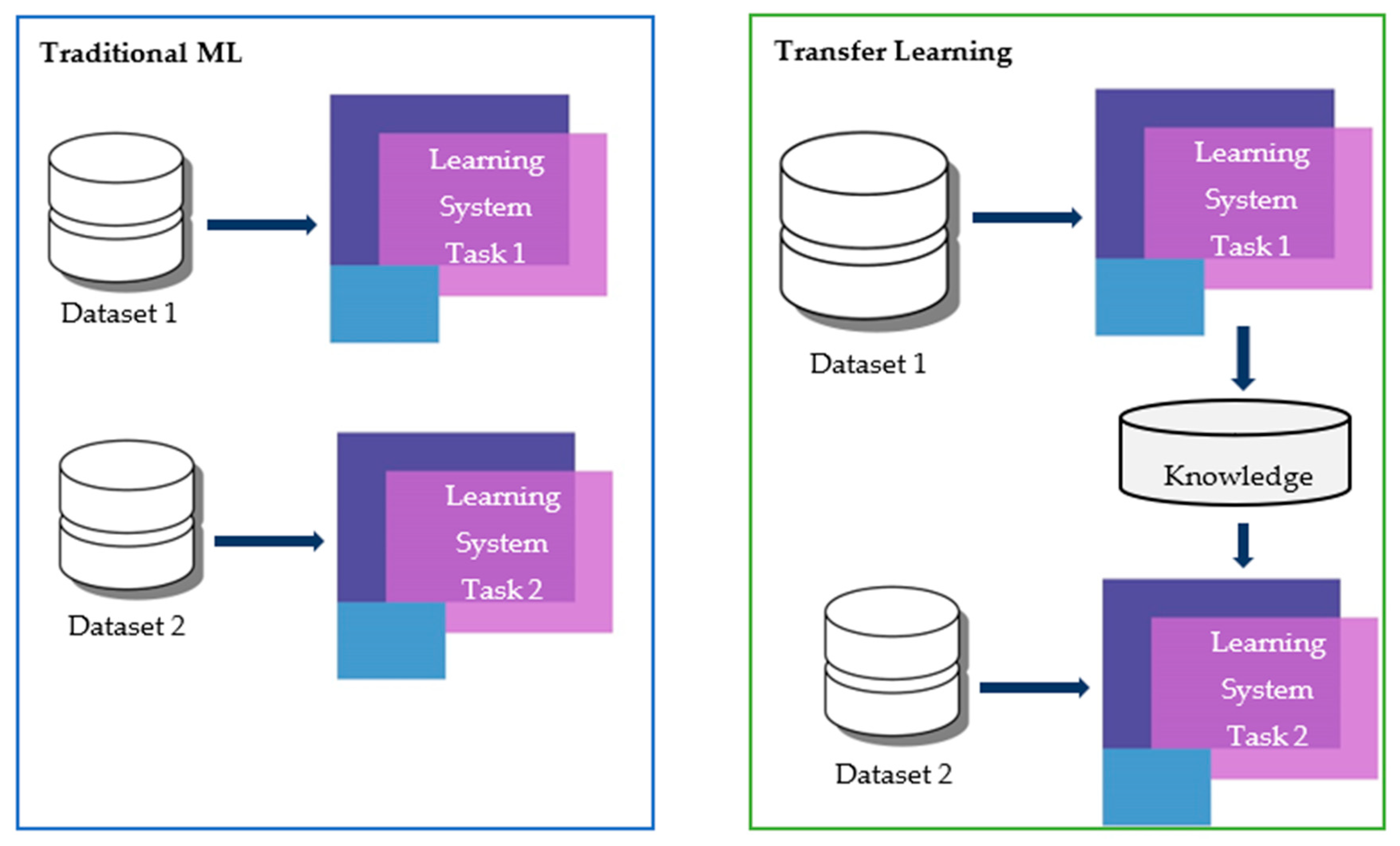
6. What is Transfer Learning?

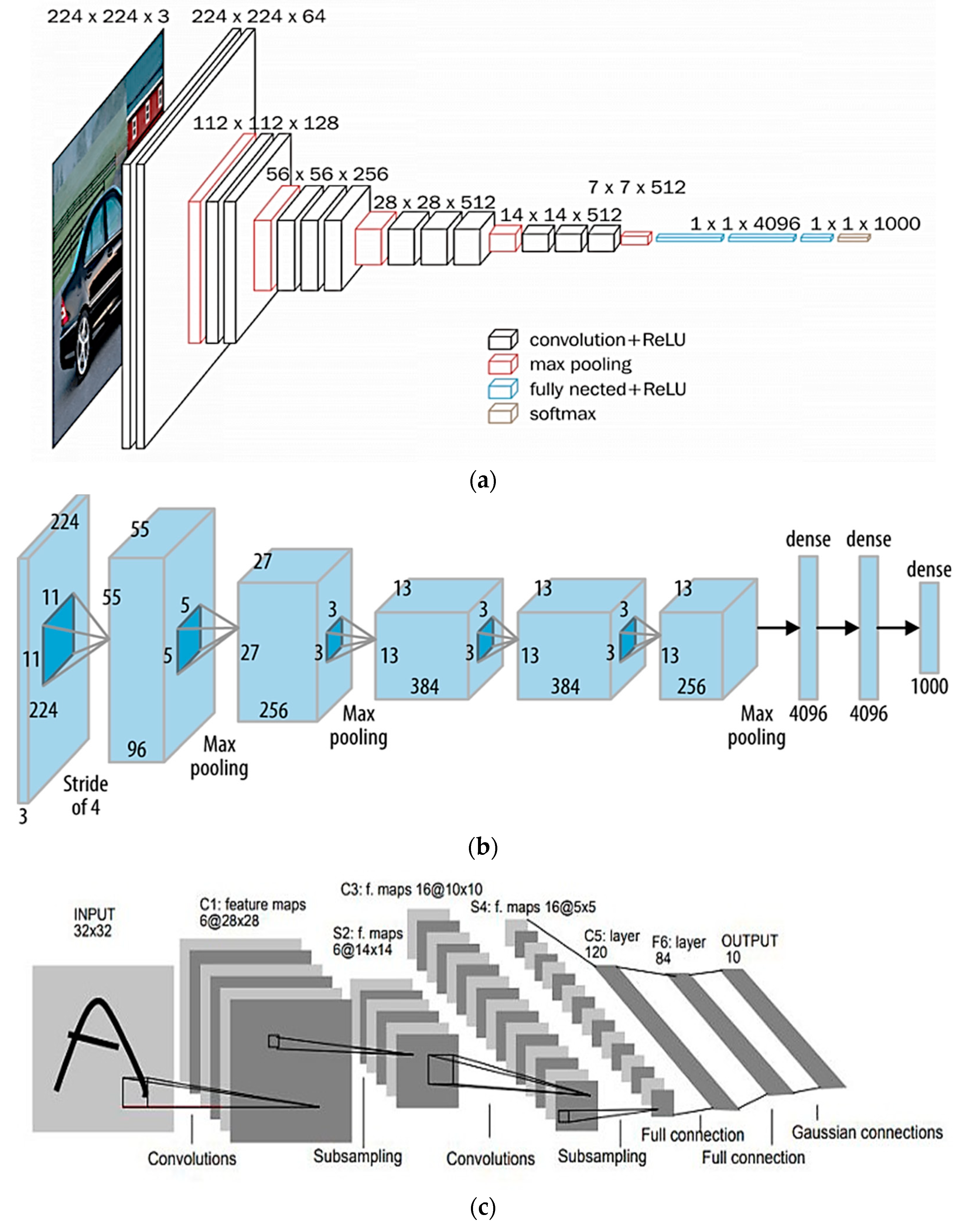
Transfer learning is a method of learning where a model learns about one problem before this serves as the starting point for another task. This is a suitable approach for problems when a procedure near the primary issue already exists and the related task requires a lot of data [77].

Transfer learning uses the technique of feature extraction from a pre-trained model; this eliminates the need for developers to start over when training a model. A TL model is typically trained on a large dataset (for example, ImageNet) [78] and the related parameters obtained from the trained model can then be used with a custom neural network for any other related application. These types of models can be used directly for predictions on new tasks or in any other related application training processes of the model. For instance, in the process of image classification, the model, such as an ANN, which is used for prediction will be trained and learned with a large number of images or datasets of the specific domain [79], like dogs and cats. Model weights are one option for the first step in the process. The traits which the machine has previously mastered for a more extensive mission, such as retrieving shapes, patterns, and lines, are also useful for different objectives.

One more problem to consider with traditional neural networks is that when we apply these kinds of models in clinical practice, the model is likely to fail due to unseen data, which is nothing but data that is not used while training the model. Therefore, the capacity to generalize to previously encountered clinical data is still a major shortcoming of these algorithms. Another shortcoming is when the data is limited; we know that the running performance of a deep network is impacted by the amount of data. One way to overcome this shortcoming is to collect more data, specifically looking for data that is exactly supervised data. Hence, there are transfer learning techniques that may be considered as choices. Rather than starting from scratch, we can use an existing network to train a new one; LeNet-5, AlexNet, VGG-16 Net, Inception Net ResNet, and DenseNet have been widely used as pre-trained networks for the classification of images in medical domains. All these architectures were trained on the well-known dataset (ImageNet) [80] consisting of 1000 object category classifications [81]. There are more than a million images in ImageNet’s training set, around fifty thousand in its validation set, and one hundred thousand in its test set. [82]. These models not only reduce training time but also reduce generalization errors.

Table 2. A brief description of traditional ML vs transfer learning.

Traditional ML	Transfer Learning
Isolated, single task learning Knowledge is not retained or accumulated. Learning is performed without consideration for knowledge learned from other tasks.	The learning of new activities is dependent on previously learnt ones The learning process could be more efficient, more accurate, or need fewer training data sets.

shows the main differences between traditional ML and transfer learning.

6.1. LeNet5

In 1889, Yann LeCun et al. published a paper that proposed a technique for document recognition which is called gradient-based learning [83]; their work described LeNet-5, which was probably the first widely recognized and effective implementation of CNN. The author trained the model for the recognition of handwritten characters based on a standard famous dataset called MNIST (Modified National Institute of Standards and Technology dataset). As a result, a significant classification result of 99.2% accuracy and a low error rate was achieved. The LeNet-5 architecture receives the input image as a grayscale 32 × 32 image size, and the model is a composite of seven layers, including layers of convolution and average pooling followed by a layer that is fully connected. Figure 5 shows the comparison transfer learning and transfer machine learning. Figure 6b depicts the LeNet-5 architecture. Interestingly, in LeNet-5, the filters used for capturing feature maps are increased as the network progresses in depth [81].

Key facts:

• This network is very easy to understand and served as a good introduction to the field of neural networks. Character recognition works well.
• Due to the shallowness (not deep enough) of the model, it has a difficult time searching for all features, leading to models with poor performance.
• This model does not work with color images.

6.2. AlexNet

In 2012, another researcher named Alex Krizhevsky, and his co-workers developed a model known as AlexNet [84]. The paper proposed and discussed the deep ConvNets for the classification of ImageNet. This was done due to a competition in 2010 called the ILSVRC (ImageNet Large-Scale Visual Recognition Challenge) [85], whose purpose was to detect and classify objects. This was where, later on, the importance of image classification using CNNs became the buzzword. AlexNet is like LeNet but much larger and with a greater number of filters for each layer. Another major change in AlexNet was to replace the traditional S-shaped functions, like Tanh or logistic, with new nonlinear functions called ReLU (rectified linear), which are placed after every convolutional layer. Additionally, in the output layer of AlexNet, another activation function called Softmax is placed, Figure 6c shows AlexNet architecture. Moreover, this model uses the max-pooling technique instead of average pooling, and a new method called dropout has been utilized between the fully connected layers to address overfitting and enhance generalization error. The AlexNet architecture takes a fixed input of 224x224x3 size and is built upon eight layers. In total, five layers go to convolutional operations and three layers go to fully connected operations.

Key facts:

• The first significant CNN model to use GPU training, which leads to faster training, was AlexNet.
• In comparison to another model like LeNet, the AlexNet model has eight layers and a deeper structural design, making it better able to extract important features. It also performed admirably for color images.
• As compared to future models, it takes longer to obtain results with high accuracy with AlexNet.

6.3. VGG Net

In 2014 [85], two Oxford researchers at the Visual Geometry Group lab came up with an idea of a much deeper CNN with better performance named VGG; this again happened through the ILSVRC 2014 [57] competition. There are different variants of the VGG net architecture, such as the VGG-19 and the VGG-16. Their names refer to the number of learned layers in the architecture. In VGG, before max pooling is performed, several convolutional layers are stacked together, such as two, three, and even four. The reason for stacking the conv-layers together is to define a block. The employment of many tiny filters is the first significant change that has a de facto standard; this CNN utilizes filters of size 1 × 1 and 3 × 3, and a stride of one, as opposed to LeNet-5′s large filters. The number of filters rises with the mode’s depth, starting at 64 and increasing to 128, 256, and 512 filters after extracting features from the model. Figure 6a represent the architecture of VGG Net

Key facts:

• VGG is simple to comprehend and explain.
• A baseline of about 80 percent is recommended for classic problems like classifying cats and dogs.
• A longer inference time is caused by the greater number of weight parameters.

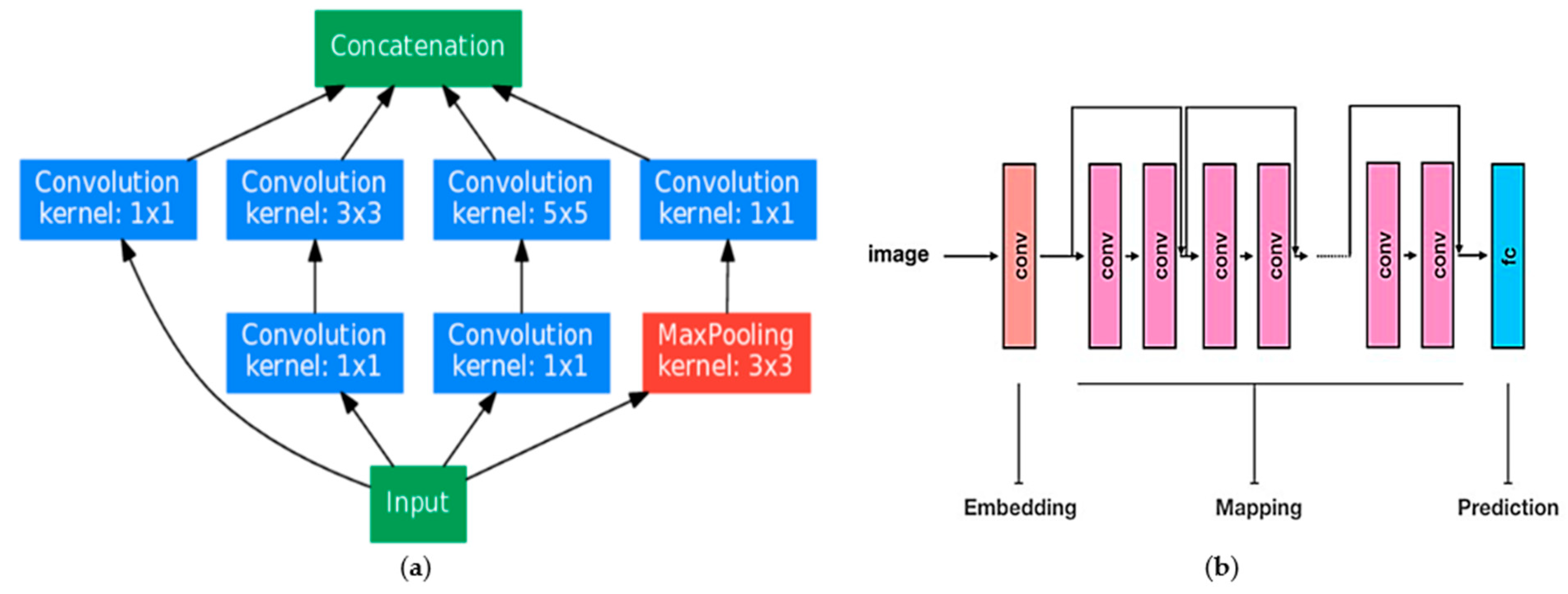
6.4. Inception Net

Christian Szegedy et al. published a paper titled “Going Deeper with Convolutions” [85], which described another complex and heavily engineered architecture named the Inception network. The key goal of the author was to use a lot of techniques to increase performance in terms of precision, accuracy, and speed. The network’s ongoing evolution resulted in the production of multiple versions, such as Inception v1, v2, and v3 [86]. Each new version is a step forward from the preceding one [81]. The Inception module is the major innovative element in this network, the model architecture is given in Figure 7a. It is nothing but a parallel block of convolutional layers consisting of 3 different kernel sizes such as 5 × 5, 1 × 1, and 3 × 3, with a max-pooling layer of 3 × 3. Further, all the results are concatenated. Version 3 of Inception, which is an optimized and upgraded version of Inception, is made of 42 layers and, compared to other versions, it has a lower error rate [81].

Key facts:

• As a result of applying multiple convolution filters to the same input in the case of multi-level feature extraction, computational costs are reduced.
• Increased performance can be achieved on this CNN.
• Inception model can be train more quickly than the VGG model and VGG model is relatively bigger in size as compared to LeNet-5.

6.5. ResNet

Image recognition is further considered using deep residual learning by Kaiming He et al. in 2016 [81]. The ResNet152V2 is built with a total number of 152 layers, and the concept of residual blocks in the network that utilize shortcut connections is crucial to the mode’s construction. A residual block is a combination of two conv-layers with an activation function, such as ReLU. The problem of vanishing gradient which exists in deep networks is solved by ResNet skip-or-shortcut connections by letting the gradient flow through an additional path (shortcut path) [81]. The main difference between ResNet v1 and v2 is that the batch-normalization technique is applied before each weight layer. Architecture of Resnet is depicted in Figure 7a.

Key facts:

• Skip-or-shortcut connections aid in addressing the issue of vanishing gradients.
• The structure increases the training pace.
• ResNet provides greater accuracy, particularly in classification.
• It makes an effort to distinguish between learned features, and if a learned feature is not relevant to the decision at hand, its weight is reduced to zero.
• Since it is incorporating skip connections between layers that may take dimensionality into account, it also increases architectural complexity [78].

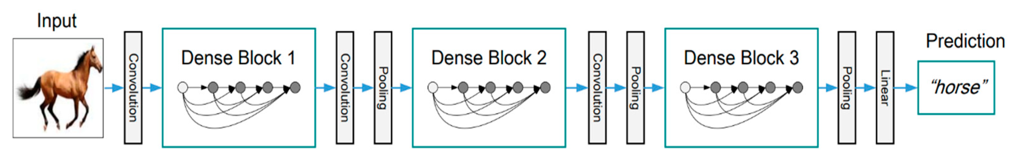
6.6. DenseNet

Gao Huang and colleagues developed the DenseNet in 2017, which consists of layers that are densely connected to one another and are all associated with one another. This method helps to reuse features, because each layer obtains its input from the levels that came before it and produces its feature mappings to be used by the layers that come after it. Additionally, each layer provides its input to all subsequent layers. The structure of DenseNet includes two dense blocks with two transition blocks in between each pair of dense blocks. Figure 8 shows the DenseNet architecture. [87]. The following are important concepts in DenseNet:

• Growth rate: This determines the number of feature maps that are output into individual layers within dense blocks;
• Dense connectivity: Dense connectivity refers to the fact that within a dense block, each successive layer is able to obtain input feature maps from the layer below it [88];
• Composite functions: The following is an explanation of the order in which operations take place within a layer. First, we begin with batch normalization, then move on to applying activation functions (e.g., ReLU), and finally, arrive at the convolution layer [87];
• Transition layers: The transition layers reduce the dimensions of the dense block by aggregating the feature maps that are contained within it. Therefore, maximum pooling has been enabled.

Key facts:

• Each subsequent layer adds only a small number of parameters; for example, only about 12 kernels are learned in each subsequent layer. Therefore, parameter efficiency is achieved.
• Better distribution of the gradient throughout the network for all of the feature maps can enable the CNN to directly access the loss function and its gradient, which gives implicit deep supervision [89].

Figure 7. (a) Building blocks of the Inception architecture; (b) Three building elements make up the ResNet architecture in a schematic: embedding, mapping, and prediction. Convolution procedures and nonlinear activations are described by the terms “conv” and “fc,” respectively [90,91].

Figure 7. (a) Building blocks of the Inception architecture; (b) Three building elements make up the ResNet architecture in a schematic: embedding, mapping, and prediction. Convolution procedures and nonlinear activations are described by the terms “conv” and “fc,” respectively [90,91].

Figure 8. Architecture of DenseNet.

Figure 8. Architecture of DenseNet.

7. Practical Perspective and Fine-Tuning of Transfer Learning Techniques

• Training the entire model: In this approach, the entire pre-trained model is used as a starting point, and all the parameters of the model are fine-tuned for the new task. This is suitable when the new task is similar to the original task for which the pre-trained model was trained [92].
• Freezing some layers: In this approach, some of the layers in the pre-trained model are frozen and the remaining layers are fine-tuned for the new task. Typically, the lower-level layers of the pre-trained model, which capture low-level features such as edges and corners, are frozen, while the higher-level layers, which capture more complex features, are fine-tuned. This is suitable when the new task is related to the original task but requires some modification of the model [93].
• Fine-tuning some layers: In this approach, some of the layers in the pre-trained model are fine-tuned while the remaining layers are frozen. Typically, the higher-level layers of the pre-trained model, which capture more complex features, are fine-tuned, while the lower-level layers are frozen. This is suitable when the new task is significantly different from the original task, but the higher-level features of the pre-trained model can still be useful [93].
• Freezing the convolutional base: In this approach, the convolutional base of the pre-trained model is frozen, and a new classifier is added on top of it. The new classifier is then trained on the new task [94]. This is suitable when the new task requires a different classification scheme than the original task, but the pre-trained convolutional base can still be used to extract features from the input data [95].

In general, transfer learning can be a powerful tool for machine learning tasks, as it allows for the reuse of pre-trained models that have already learned useful representations from large amounts of data. The appropriate transfer learning method will depend on the specifics of the new task and the pre-trained model. To choose a pre-trained model for your problem, you can select from a variety of options such as VGG [96], InceptionV3 [97], ResNet5, DenseNet, and so on.

8. Important Things for Consideration

8.1. Generalization: Problems and Key Concepts to Mitigate

We say that a model generalizes well if the model is tested on unlabeled data after training on known labeled data and the machine performs well on testing data. However, when a network performs well on the training set, but poorly overall, it is said to overfit [98]. This problem is common in deep learning models because there are so many parameters for the model to learn; therefore, these types of models are prone to overfitting.

One of the hardest problems is enhancing the generalization capability to prevent the overfitting of machine or deep learning models. Plotting the training and validation accuracy rate at each iteration during training is one method of identifying overfitting [99].

• Data augmentation: One approach to avoid overfitting is to simply expand the quantity of data, However, gathering large amounts of data in real-world situations is a laborious and time-consuming task, so collecting new data is not a practical option. Increasing the total size of the dataset [37] used for training is one of the best methods for reducing overfitting. Since we are talking about CNNs for image-based data, the easiest way to add variety to our data and expand it is to add more images to the dataset. This process is referred to as data augmentation [100]. This has potential for narrowing the gap between the training and validation set, as well as between those two sets and any future test sets [98], because the augmented data will represent a comprehensive collection of possible data points. Therefore, augmentation is a highly effective strategy.

Several other common techniques that have been used to tackle the overfitting problem are listed below:

• Batch normalization: This approach is the one that is utilized most frequently in deep learning, as it increases the speed at which neural networks learn new information and provides regularization, thereby preventing the problem of overfitting. In CNN convolutions, shared filters follow input feature maps and are the same on every feature map [101]. When this occurs, it is reasonable to normalize the output in the same manner, and then share it across the feature maps. Therefore, each map will have a single standard deviation and mean for all its features [102];
• Dropout: This is a training method in which some neurons are selectively ignored. A model with applied dropout cannot rely on any single feature and must instead learn robust features. This method has been shown to effectively decrease overfitting in numerous issues [103]. Tompson [104] expanded on this concept by applying it to a convolutional neural network using a technique called spatial dropout. This technique eliminates entire feature maps as opposed to individual neurons;
• Weight decay: In model training, large weights mean that the prediction relies heavily on one pixel; therefore, a more interesting method comes to the picture, which is weight decay, which says that large weights are penalized [105]. Intuitively, the classification of an image based on one or a few pixels seems to not make sense;
• Transfer learning: This involves training a machine model on a large amount of data like ImageNet and using those weights in a new classification task [106].

8.2. Computational Accelerators within the Scope of DL

The majority of ConvNets have extremely high memory and computation requirements, particularly while they are being trained. As a result, this should be one of your primary concerns. For example, deploying a model to run locally on mobile, you should give careful consideration to the size of the trained model after it has been completed. Increasing the amount of computational work done by a network is necessary to achieve higher levels of accuracy [59]. Therefore, there is always a compromise that needs to be made between accuracy and computational speed. In addition to these factors, there are a great number of other considerations, such as the simplicity of training, the capacity of a network to generalize data effectively, etc.

It is stated [107] that the increased ratio of the total amount of layers accumulated over time appears to be significantly quicker than the growth ratio predicted by Moore’s Law. The use of graphics processing units (GPUs) and tensor processing units (TPUs) acts as a means of enhancing the performance of central processing units (CPUs) when running deep nets; therefore, it is necessary to have an understanding of the technologies that underpin the CPU, GPU, and TPU in order to maintain a competitive edge in terms of both performance and efficiency.

The main difference between CPU, GPU, and TPU is thatwhile the CPU is used for general-purpose processing, the GPU and TPU, on the other hand, are more like the computer’s muscles. GPUis a performance accelerator that helps computer graphics and artificial intelligence work [108], while TPUs are Google’s processors designed to speed up machine learning tasks using frameworks such as TensorFlow.

9. Discussion

Medical imaging is an essential tool that unites societal and scientific requirements and can create a significant synergy that could promote research in both fields. Machine learning, particularly deep learning (DL), is a fast-moving research subject with promising imaging and therapeutic applications. DL has already permeated medical image analysis. Although recent advances in DL approaches have been astounding, there are still obstacles to their implementation in healthcare. Because it does not leave an audit trail to explain the decisions it makes, DL is often referred to as a black box. Image analysis was not meant to replace radiologists, but to serve as a second opinion. There is no denying that improvements in the digital imaging industry have had and will continue to have a favorable impact on medical imaging. CNNs have positively contributed to many fields, including medical research and radiology, and they are becoming more and more popular. As a result, with the capability to learn high-level features from medical images without requiring a step of feature engineering, they become a viable alternative to machine learning algorithms. In this manuscript, a comprehensive review of the strengths, performance, and limitations of the latest DL-based approaches is presented [109] for applications dealing with medical imaging domains.

As per the data from MetaAI [110], we have found that the majority of work has been done on classification problems, specifically in image classification as shown in below Figure 9 [111].

We also determined that, after reviewing many research articles, the most common and efficient activation function which has been adopted in the building of CNN is ReLU. In the field of DL, ReLU is a non-linear function, meaning that it converts all negative values to 0, and it has become an increasingly prominent activation function. The primary benefit that the ReLU function has over other activations is that it does not fire all of the neurons at the same time, as other functions do [112]. This is mostly used on every conv-layer, as well as each and every dense layer [113]. The following are the most common reasons behind using this activation function:

• Vanishing gradient: Since the derivative of this activation can only be either on the value 0 or 1, it cannot fall within the range [0, 1] [114]. As a consequence of this result, the product of various derivatives would also be either 0 or 1. Therefore, the problem of vanishing gradients does not arise when backpropagation is being performed;
• Sparsity: An ReLU will always produce an output value of 0 in response to negative input. This indicates that a smaller percentage of the network’s neurons are actively firing. As a result, the neural network possesses activations that are both sparse and efficient;
• Speedier training: Better convergence performance is typically demonstrated by networks that have the ReLU function and offer faster training. As a result, our total running time is significantly shorter [111].

Even though there are a few methods, like the ones listed above, that make it easier to learn from smaller datasets, it is still important to have large, well-annotated medical datasets because most of the big achievements of deep learning are usually based on huge datasets. Building these kinds of medical datasets is expensive, takes a lot of work from experts, and may have ethical and privacy problems. However, once such datasets are made accessible, specialized medical pre-trained networks would likely be presented, which might encourage deep-learning research on medical imaging.

• Furthermore, due to the complex structures of data, training a deep learning model is extremely expensive. They often require expensive GPUs and a large number of computers, which raises the cost for users.
• Training performance worsens as a result of the large computational load required by the growing complexity of multiple layers. To tackle the vanishing gradient issue, over-fitting concerns, improved activation, and cost function design, dropout techniques have been employed [113].
• Utilizing hardware with a high degree of parallelism, such as GPUs and normalization techniques, allowed for the large computational-weight issue to be resolved [61].

From a practical point of view, transfer learning techniques for image classification problems are mainly based on the size and similarity of the dataset. The strategies are summarized into four categories as follows [92]:

• Category 1: Large dataset, but different from the pre-trained model’s dataset. Strategy 1 is recommended, which involves training a model from scratch but using the architecture and weights of a pre-trained model to initialize the model.
• Category 2: Large dataset and similar to the pre-trained model’s dataset. Any option can work, but Strategy 2 is the most efficient. This involves training the classifier and top layers of the convolutional base, leveraging previous knowledge.
• Category 3: Small dataset and different from the pre-trained model’s dataset. Strategy 2 is recommended, but it can be challenging to find the right balance between the number of layers to train and freeze. Data augmentation techniques may be necessary.
• Category 4: Small dataset, but similar to the pre-trained model’s dataset. Strategy 3 is the best option, which involves using the pre-trained model as a fixed feature extractor, removing the last fully connected layer, and training a new classifier using the resulting features.

A learning model that is subject to supervision, either for classification or regression problems, must learn from training data to produce accurate predictions. Unfortunately, the problem arises that whenever we make an effort to train a complicated model with an insufficient amount of data for training purposes, overfitting occurs [114]. Overfitting is the most critical issue in deep learning, so understanding, finding, and avoiding it is important. Researchers have described many methods to tackle this problem such as data augmentation, weight decay, transfer learning, batch normalization, dropout, etc.

As for the computational approach, is a concern. It has been demonstrated by researchers from Harvard that different platforms give advantages to different models based on their individual qualities. These advantages might be advantageous for the model’s overall performance. Below are the key takeaways:

• CPU: It is responsible for achieving the highest FLOPS utilization for Recurrent Neural Networks and is capable of supporting the largest models due to its vast memory capacity;
• GPU: For irregular computations, such as tiny batches and nonMatMul computations, the GPU demonstrates more flexibility and programmability than other processing units;
• TPU: It is highly optimized for large batches and boasts the best possible training throughput.

10. Conclusions

This article gives people in the field of DL a place to start. It could also help them to choose the best way to go about their work in order to come up with more accurate models. The study further provides an analysis of the various architectures of CNNs used in the classification of medical images, and also demonstrates how developments in deep learning algorithms produce promising findings that can assist and act as a second eye to many radiologists. CNN-based architectures have been utilized in the medical domain in various disease detection and prediction cases. The following points are given to wrap up our review and show where things are going in the current and the future.

• To make accurate predictions and train deep learning models, these models need access to large datasets, preferably with labels. When processing data in real-time is necessary, to be specific in the case of healthcare data, this problem becomes more difficult. Over the past few years, researchers have investigated potential solutions to this problem, such as data augmentation and pre-trained CNN models.
• Changes to the hyperparameter settings will have a significant impact on the deep learning-based models’ overall performance. Therefore, developing an optimization technique requires careful consideration of parameter choices; for example, there are various techniques to mitigate this problem such as Keras Tuner, Ray Tuner, etc.
• In order to train a CNN model effectively, powerful computational approaches are required like GPUs or TPUs. Therefore, there is a significant amount of ongoing work being conducted to think of ways to speed up these resources.
• Generalizability of the CNN in the case of medical imaging is very important; therefore, concepts like dropout, batch-normalization, weight decay, transfer learning, and data augmentation are presented.
• To find the solution to not having enough data for training, we discussed data augmentation, which is one way to help in the creation of more data from the existing data, and it is likely that different pre-trained CNN models will utilize this solution. For example, a CNN could be trained on a huge amount of unlabeled data, and then that knowledge could be used to train that CNN on a smaller amount of labeled data for the same job.
• It is anticipated that a variety of approaches to learning through transfer will be taken into consideration and choosing the right strategy for utilizing such models in image classification depends on the similarity and the amount of the dataset.
• While utilizing a CNN alone can be computationally costly, using transfer learning with pre-trained CNN models can greatly lower the cost of training a CNN for medical imaging diagnosis while simultaneously enhancing its performance.

References

1. Cai, L.; Gao, J.; Zhao, D. A review of the application of deep learning in medical image classification and segmentation. Ann. Transl. Med. 2020, 8, 713. [Google Scholar] [CrossRef]
2. Chopra, P.; Junath, N.; Singh, S.K.; Khan, S.; Sugumar, R.; Bhowmick, M. Cyclic GAN Model to Classify Breast Cancer Data for Pathological Healthcare Task. BioMed Res. Int. 2022, 2022, 6336700. [Google Scholar] [CrossRef] [PubMed]
3. Zhou, S.K.; Greenspan, H.; Davatzikos, C.; Duncan, J.S.; Van Ginneken, B.; Madabhushi, A.; Prince, J.L.; Rueckert, D.; Summers, R.M. A Review of Deep Learning in Medical Imaging: Imaging Traits, Technology Trends, Case Studies with Progress Highlights, and Future Promises. Proc. IEEE 2021, 109, 820–838. [Google Scholar] [CrossRef]
4. Dutta, P.; Upadhyay, P.; De, M.; Khalkar, R. Medical Image Analysis using Deep Convolutional Neural Networks: CNN Architectures and Transfer Learning. In Proceedings of the 5th International Conference on Inventive Computation Technologies, ICICT 2020, Coimbatore, India, 26–28 February 2020; pp. 175–180. [Google Scholar] [CrossRef]
5. Singh, S.P.; Wang, L.; Gupta, S.; Goli, H.; Padmanabhan, P.; Gulyás, B. 3D Deep Learning on Medical Images: A Review. Sensors 2020, 20, 5097. [Google Scholar] [CrossRef] [PubMed]
6. Guezzaz, A.; Azrour, M.; Benkirane, S.; Mohy-Eddine, M.; Attou, H.; Douiba, M. A Lightweight Hybrid Intrusion Detection Framework Using Machine Learning for Edge-Based IIoT Security. Int. Arab. J. Inf. Technol. 2022, 19, 822–830. [Google Scholar] [CrossRef]
7. Khan, S. Business Intelligence Aspect for Emotions and Sentiments Analysis. In Proceedings of the 2022 First International Conference on Electrical, Electronics, Information and Communication Technologies (ICEEICT), Trichy, India, 16–18 February 2022; pp. 1–5. [Google Scholar] [CrossRef]
8. Khan, S.; Fazil, M.; Sejwal, V.K.; Alshara, M.A.; Alotaibi, R.M.; Kamal, A.; Baig, A.R. BiCHAT: BiLSTM with deep CNN and hierarchical attention for hate speech detection. J. King Saud Univ. Comput. Inf. Sci. 2022, 34, 4335–4344. [Google Scholar] [CrossRef]
9. Azrour, M.; Mabrouki, J.; Fattah, G.; Guezzaz, A.; Aziz, F. Machine learning algorithms for efficient water quality prediction. Model. Earth Syst. Environ. 2021, 8, 2793–2801. [Google Scholar] [CrossRef]
10. Mutasa, S.; Sun, S.; Ha, R. Understanding artificial intelligence based radiology studies: CNN architecture. Clin. Imaging 2021, 80, 72–76. [Google Scholar] [CrossRef]
11. Lee, J.-G.; Jun, S.; Cho, Y.-W.; Lee, H.; Kim, G.B.; Seo, J.B.; Kim, N. Deep Learning in Medical Imaging: General Overview. Korean J. Radiol. 2017, 18, 570–584. [Google Scholar] [CrossRef] [Green Version]
12. Bhatt, D.; Patel, C.; Talsania, H.; Patel, J.; Vaghela, R.; Pandya, S.; Modi, K.; Ghayvat, H. CNN Variants for Computer Vision: History, Architecture, Application, Challenges and Future Scope. Electronics 2021, 10, 2470. [Google Scholar] [CrossRef]
13. Kim, M.; Yun, J.; Cho, Y.; Shin, K.; Jang, R.; Bae, H.-J.; Kim, N. Deep Learning in Medical Imaging. Neurospine 2019, 16, 657–668. [Google Scholar] [CrossRef] [Green Version]
14. Haq, A.U.; Li, J.P.; Khan, I.; Agbley, B.L.Y.; Ahmad, S.; Uddin, M.I.; Zhou, W.; Khan, S.; Alam, I. DEBCM: Deep Learning-Based Enhanced Breast Invasive Ductal Carcinoma Classification Model in IoMT Healthcare Systems. IEEE J. Biomed. Health Inform. 2022, 1–12. [Google Scholar] [CrossRef]
15. Abdelhafiz, D.; Yang, C.; Ammar, R.; Nabavi, S. Deep convolutional neural networks for mammography: Advances, challenges and applications. BMC Bioinform. 2019, 20, 281. [Google Scholar] [CrossRef] [PubMed] [Green Version]
16. Salehi, W.; Gupta, G.; Bhatia, S.; Koundal, D.; Mashat, A.; Belay, A. IoT-Based Wearable Devices for Patients Suffering from Alzheimer Disease. Contrast Media Mol. Imaging 2022, 2022, 3224939. [Google Scholar] [CrossRef] [PubMed]
17. IEEE. 2017 IEEE 19th International Conference on e-Health Networking, Applications and Services (Healthcom); IEEE: Piscataway, NJ, USA, 2017. [Google Scholar]
18. Kushnure, D.T.; Tyagi, S.; Talbar, S.N. LiM-Net: Lightweight multi-level multiscale network with deep residual learning for automatic liver segmentation in CT images. Biomed. Signal Process. Control. 2023, 80, 104305. [Google Scholar] [CrossRef]
19. Haq, A.U.; Li, J.P.; Khan, S.; Alshara, M.A.; Alotaibi, R.M.; Mawuli, C. DACBT: Deep learning approach for classification of brain tumors using MRI data in IoT healthcare environment. Sci. Rep. 2022, 12, 15331. [Google Scholar] [CrossRef] [PubMed]
20. Torres-Velazquez, M.; Chen, W.-J.; Li, X.; McMillan, A.B. Application and Construction of Deep Learning Networks in Medical Imaging. IEEE Trans. Radiat. Plasma Med. Sci. 2020, 5, 137–159. [Google Scholar] [CrossRef]
21. Mukhlif, A.A.; Al-Khateeb, B.; Mohammed, M.A. An extensive review of state-of-the-art transfer learning techniques used in medical imaging: Open issues and challenges. J. Intell. Syst. 2022, 31, 1085–1111. [Google Scholar] [CrossRef]
22. Wiesel, T.N. Receptive fields and functional architecture of monkey striate cortex. J. Physiol. 1968, 195, 215–243. [Google Scholar]
23. Ghosh, A.; Sufian, A.; Sultana, F.; Chakrabarti, A.; De, D. Fundamental Concepts of Convolutional Neural Network. In Recent Trends and Advances in Artificial Intelligence and Internet of Things; Springer: Berlin/Heidelberg, Germany, 2019; pp. 519–567. [Google Scholar] [CrossRef]
24. Fukushima, K.; Miyake, S. Neocognitron learning by backpropagation. Syst. Comput. Jpn. 1995, 26, 19–28. [Google Scholar] [CrossRef]
25. Khan, S.; Kamal, A.; Fazil, M.; Alshara, M.A.; Sejwal, V.K.; Alotaibi, R.M.; Baig, A.R.; Alqahtani, S. HCovBi-Caps: Hate Speech Detection Using Convolutional and Bi-Directional Gated Recurrent Unit with Capsule Network. IEEE Access 2022, 10, 7881–7894. [Google Scholar] [CrossRef]
26. Jogin, M.; Mohana; Madhulika, M.S.; Divya, G.D.; Meghana, R.K.; Apoorva, S. Feature Extraction using Convolution Neural Networks (CNN) and Deep Learning. In Proceedings of the 2018 3rd IEEE International Conference on Recent Trends in Electronics, Information and Communication Technology, RTEICT 2018, Bangalore, India, 18–19 May 2018; pp. 2319–2323. [Google Scholar] [CrossRef]
27. Zhang, S.; Zhang, M.; Ma, S.; Wang, Q.; Qu, Y.; Sun, Z.; Yang, T. Research Progress of Deep Learning in the Diagnosis and Prevention of Stroke. BioMed Res. Int. 2021, 2021, 5213550. [Google Scholar] [CrossRef] [PubMed]
28. Brownlee, J. A Gentle Introduction to Pooling Layers for Convolutional Neural Networks. Mach. Learn. Mastery 2019, 22. Available online: https://machinelearningmastery.com/pooling-layers-for-convolutional-neural-networks/ (accessed on 5 December 2022).
29. Naranjo-Torres, J.; Mora, M.; Hernández-García, R.; Barrientos, R.J.; Fredes, C.; Valenzuela, A. A Review of Convolutional Neural Network Applied to Fruit Image Processing. Appl. Sci. 2020, 10, 3443. [Google Scholar] [CrossRef]
30. Sun, M.; Song, Z.; Jiang, X.; Pan, J.; Pang, Y. Learning Pooling for Convolutional Neural Network. Neurocomputing 2017, 224, 96–104. [Google Scholar] [CrossRef]
31. Liu, T.; Fang, S.; Zhao, Y.; Wang, P.; Zhang, J. Implementation of Training Convolutional Neural Networks. arXiv 2015, arXiv:1506.01195, preprint. [Google Scholar]
32. Mac, S.; Products, S.; Also, C. Convolutional Kernel Networks Julien. arXiv 2014, arXiv:1406.3332, preprint. [Google Scholar]
33. Corvil. The Role of Bias in Neural Networks. 2018. Available online: https://www.pico.net/kb/the-role-of-bias-in-neural-networks/ (accessed on 16 March 2022).
34. Skalski, P. Gentle Dive into Math Behind Convolutional Neural Networks. Data Sci. 2019. Available online: https://towardsdatascience.com/https-medium-com-piotr-skalski92-deep-dive-into-deep-networks-math-17660bc376ba (accessed on 20 February 2023).
35. Hashemi, M. Enlarging smaller images before inputting into convolutional neural network: Zero-padding vs. interpolation. J. Big Data 2019, 6, 1–13. [Google Scholar] [CrossRef] [Green Version]
36. Prabhu. Understanding of Convolutional Neural Network (CNN)—Deep Learning. Medium. 2022. Available online: https://medium.com/@RaghavPrabhu/understanding-of-convolutional-neural-network-cnn-deep-learning-99760835f148 (accessed on 15 February 2023).
37. Srivastava, N.; Hinton, G.; Krizhevsky, A.; Sutskever, I.; Salakhutdinov, R. Dropout: A Simple Way to Prevent Neural Networks from Overfitting. J. Mach. Learn. Res. 2014, 15, 1929–1958. [Google Scholar]
38. Adrian, G. Dropout in Recurrent Neural Networks. 2018. Available online: https://adriangcoder.medium.com/a-review-of-dropout-as-applied-to-rnns-72e79ecd5b7b (accessed on 12 October 2022).
39. Radhakrishnan, P. What are Hyperparameters? And How to tune the Hyperparameters in a Deep Neural Network? Data Sci. 2017. Available online: https://towardsdatascience.com/what-are-hyperparameters-and-how-to-tune-the-hyperparameters-in-a-deep-neural-network-d0604917584a (accessed on 20 February 2023).
40. Sharma, S.; Sharma, S.; Anidhya, A. Understanding Activation Functions in Neural Networks. Int. J. Eng. Appl. Sci. Technol. 2020, 4, 310–316. [Google Scholar]
41. Nwankpa, C.; Ijomah, W.; Gachagan, A.; Marshall, S. Activation Functions: Comparison of trends in Practice and Research for Deep Learning. arXiv 2018, arXiv:1811.03378. preprint. [Google Scholar]
42. Neal, R.M. Connectionist learning of belief networks. Artif. Intell. 1992, 56, 71–113. [Google Scholar] [CrossRef]
43. DeepAI. ReLu Definition. In Deep AI Machine Learning Glossary; DeepAI; Available online: https://deepai.org/machine-learning-glossary-and-terms/relu (accessed on 22 February 2023).
44. Agostinelli, F.; Hoffman, M.; Sadowski, P.; Baldi, P. Learning activation functions to improve deep neural networks. In Proceedings of the 3rd International Conference on Learning Representations, ICLR 2015—Workshop Track Proceedings, San Diego, CA, USA, 7–9 May 2015; pp. 1–9. [Google Scholar]
45. IEEE. Engineering in Medicine and Biology Society. In Proceedings of the IECBES, IEEE-EMBS Conference on Biomedical Engineering and Science, Kuching, Malaysia, 3–6 December 2018. [Google Scholar]
46. Khan, S.; AlSuwaidan, L. Agricultural monitoring system in video surveillance object detection using feature extraction and classification by deep learning techniques. Comput. Electr. Eng. 2022, 102, 108201. [Google Scholar] [CrossRef]
47. Boutahir, M.K.; Farhaoui, Y.; Azrour, M. Machine Learning and Deep Learning Applications for Solar Radiation Predictions Review: Morocco as a Case of Study. In Digital Economy, Business Analytics, and Big Data Analytics Applications; Springer: Berlin/Heidelberg, Germany, 2022; pp. 55–67. [Google Scholar] [CrossRef]
48. Alzubaidi, L.; Zhang, J.; Humaidi, A.J.; Al-Dujaili, A.; Duan, Y.; Al-Shamma, O.; Santamaría, J.; Fadhel, M.A.; Al-Amidie, M.; Farhan, L. Review of deep learning: Concepts, CNN architectures, challenges, applications, future directions. J. Big Data 2021, 8, 53. [Google Scholar] [CrossRef]
49. Jain, R.; Jain, N.; Aggarwal, A.; Hemanth, D.J. Convolutional neural network based Alzheimer’s disease classification from magnetic resonance brain images. Cogn. Syst. Res. 2019, 57, 147–159. [Google Scholar] [CrossRef]
50. Wu, H.; Yin, H.; Chen, H.; Sun, M.; Liu, X.; Yu, Y.; Tang, Y.; Long, H.; Zhang, B.; Zhang, J.; et al. A Deep Learning, Image Based Approach for Automated Diagnosis for Inflammatory Skin Diseases. Available online: https://www.ncbi.nlm.nih.gov/pmc/articles/PMC7290553 (accessed on 5 December 2022).
51. Ting, D.S.W.; Cheung, C.Y.-L.; Lim, G.; Tan, G.S.W.; Quang, N.D.; Gan, A.; Hamzah, H.; Garcia-Franco, R.; Yeo, I.Y.S.; Lee, S.Y.; et al. Development and Validation of a Deep Learning System for Diabetic Retinopathy and Related Eye Diseases Using Retinal Images from Multiethnic Populations with Diabetes. JAMA 2017, 318, 2211–2223. [Google Scholar] [CrossRef]
52. Gu, H.; Guo, Y.; Gu, L.; Wei, A.; Xie, S.; Ye, Z.; Xu, J.; Zhou, X.; Lu, Y.; Liu, X.; et al. Deep Learning for Identifying Corneal Diseases from Ocular Surface Slit-Lamp Photographs. Available online: https://www.nature.com/articles/s41598-020-75027-3 (accessed on 5 December 2022).
53. Bai, X.; Niwas, S.I.; Lin, W.; Ju, B.-F.; Kwoh, C.K.; Wang, L.; Sng, C.C.; Aquino, M.C.; Chew, P.T.K. Learning ECOC Code Matrix for Multiclass Classification with Application to Glaucoma Diagnosis. J. Med. Syst. 2016, 40, 78. [Google Scholar] [CrossRef] [PubMed]
54. Xin, M.; Wang, Y. Research on image classification model based on deep convolution neural network. EURASIP J. Image Video Process. 2019, 2019, 40. [Google Scholar] [CrossRef] [Green Version]
55. Brown, M.; An, P.E.; Harris, C.J.; Wang, H. How Biased is Your Multi-Layered Perceptron? World Congr. Neural Netw. 1993, 507–511. Available online: https://eprints.soton.ac.uk/250244/ (accessed on 22 February 2023).
56. Haq, A.U.H.; Li, J.P.L.; Agbley, B.L.Y.; Khan, A.; Khan, I.; Uddin, M.I.; Khan, S. IIMFCBM: Intelligent Integrated Model for Feature Extraction and Classification of Brain Tumors Using MRI Clinical Imaging Data in IoT-Healthcare. IEEE J. Biomed. Health Inform. 2022, 26, 5004–5012. [Google Scholar] [CrossRef]
57. Guezzaz, A.; Benkirane, S.; Azrour, M.; Khurram, S. A Reliable Network Intrusion Detection Approach Using Decision Tree with Enhanced Data Quality. Secur. Commun. Networks 2021, 2021, 1230593. [Google Scholar] [CrossRef]
58. ResNet; AlexNet; VGGNet. Inception: Understanding Various Architectures of Convolutional Networks. 2022. Available online: https://cv-tricks.com/cnn/understand-resnet-alexnet-vgg-inception/ (accessed on 23 February 2023).
59. Wang, P.; Fan, E.; Wang, P. Comparative analysis of image classification algorithms based on traditional machine learning and deep learning. Pattern Recognit. Lett. 2020, 141, 61–67. [Google Scholar] [CrossRef]
60. Suganyadevi, S.; Seethalakshmi, V.; Balasamy, K. A review on deep learning in medical image analysis. Int. J. Multimed. Inf. Retr. 2021, 11, 19–38. [Google Scholar] [CrossRef]
61. Shamshirband, S.; Fathi, M.; Dehzangi, A.; Chronopoulos, A.T.; Alinejad-Rokny, H. A review on deep learning approaches in healthcare systems: Taxonomies, challenges, and open issues. J. Biomed. Inform. 2020, 113, 103627. [Google Scholar] [CrossRef] [PubMed]
62. Khvostikov, A.; Aderghal, K.; Benois-Pineau, J.; Krylov, A.; Catheline, G. 3D CNN-based classification using sMRI and MD-DTI images for Alzheimer disease studies. arXiv 2018, arXiv:1801.05968, preprint. [Google Scholar]
63. Liu, Z.; Lu, H.; Pan, X.; Xu, M.; Lan, R.; Luo, X. Diagnosis of Alzheimer’s disease via an attention-based multi-scale convolutional neural network. Knowl. Based Syst. 2022, 238, 107942. [Google Scholar] [CrossRef]
64. Ajagbe, S.A.; Amuda, K.A.; Oladipupo, M.A.; Afe, O.F.; Okesola, K.I. Multi-classification of alzheimer disease on magnetic resonance images (MRI) using deep convolutional neural network (DCNN) approaches. Int. J. Adv. Comput. Res. 2021, 11, 51–60. [Google Scholar] [CrossRef]
65. Villa-Pulgarin, J.P.; Ruales-Torres, A.A.; Arias-Garz, D.; Bravo-Ortiz, M.A.; Arteaga-Arteaga, H.B.; Mora-Rubio, A.; Alzate-Grisales, J.A.; Mercado-Ruiz, E.; Hassaballah, M.; Orozco-Arias, S.; et al. Optimized Convolutional Neural Network Models for Skin Lesion Classification. Comput. Mater. Contin. 2022, 70, 2131–2148. [Google Scholar] [CrossRef]
66. Hemdan, E.E.-D.; Shouman, M.A.; Karar, M.E. COVIDX-Net: A Framework of Deep Learning Classifiers to Diagnose COVID-19 in X-ray Images. arXiv 2020, arXiv:2003.11055. preprint. [Google Scholar]
67. Horry, M.J.; Chakraborty, S.; Paul, M.; Ulhaq, A.; Pradhan, B.; Saha, M.; Shukla, N. COVID-19 Detection through Transfer Learning Using Multimodal Imaging Data. IEEE Access 2020, 8, 149808–149824. [Google Scholar] [CrossRef]
68. Joshua, E.S.N.; Bhattacharyya, D.; Chakkravarthy, M.; Byun, Y.-C. 3D CNN with Visual Insights for Early Detection of Lung Cancer Using Gradient-Weighted Class Activation. J. Healthc. Eng. 2021, 2021, 6695518. [Google Scholar] [CrossRef]
69. Li, Q.; Cai, W.; Wang, X.; Zhou, Y.; Feng, D.D.; Chen, M. Medical image classification with convolutional neural network. In Proceedings of the 2014 13th International Conference on Control Automation Robotics & Vision (ICARCV), Singapore, 10–12 December 2014; pp. 844–848. [Google Scholar]
70. Tiwari, P.; Pant, B.; Elarabawy, M.M.; Abd-Elnaby, M.; Mohd, N.; Dhiman, G.; Sharma, S. CNN Based Multiclass Brain Tumor Detection Using Medical Imaging. Comput. Intell. Neurosci. 2022, 2022, 1830010. [Google Scholar] [CrossRef] [PubMed]
71. Yildirim, M.; Cinar, A. Classification with respect to colon adenocarcinoma and colon benign tissue of colon histopathological images with a new CNN model: MA_ColonNET. Int. J. Imaging Syst. Technol. 2021, 32, 155–162. [Google Scholar] [CrossRef]
72. Ravi, V.; Narasimhan, H.; Chakraborty, C.; Pham, T.D. Deep learning-based meta-classifier approach for COVID-19 classification using CT scan and chest X-ray images. Multimed. Syst. 2021, 28, 1401–1415. [Google Scholar] [CrossRef]
73. Chakraborty, S.; Paul, S.; Hasan, K.M.A. A Transfer Learning-Based Approach with Deep CNN for COVID-19- and Pneumonia-Affected Chest X-ray Image Classification. SN Comput. Sci. 2021, 3, 17. [Google Scholar] [CrossRef] [PubMed]
74. Srinivas, C.; Prasad, N.K.S.; Zakariah, M.; Alothaibi, Y.A.; Shaukat, K.; Partibane, B.; Awal, H. Deep Transfer Learning Approaches in Performance Analysis of Brain Tumor Classification Using MRI Images. J. Healthc. Eng. 2022, 2022, 3264367. [Google Scholar] [CrossRef] [PubMed]
75. Kumar, N.; Gupta, M.; Gupta, D.; Tiwari, S. Novel deep transfer learning model for COVID-19 patient detection using X-ray chest images. J. Ambient. Intell. Humaniz. Comput. 2021, 14, 469–478. [Google Scholar] [CrossRef]
76. Vijaysinh, L. A Comparison of 4 Popular Transfer Learning Models. AIM 2021. Available online: https://arxiv.org/abs/1603.08631 (accessed on 23 February 2023).
77. Sarraf, S.; Tofighi, G. Classification of Alzheimer’s Disease Using fMRI Data and Deep Learning Convolutional Neural Networks. arXiv 2016, arXiv:1603.08631. preprint. [Google Scholar]
78. He, K.; Zhang, X.; Ren, S.; Sun, J. Deep residual learning for image recognition. In Proceedings of the IEEE Computer Society Conference on Computer Vision and Pattern Recognition (CVPR), Las Vegas, NV, USA, 27–30 June 2016; pp. 770–778. [Google Scholar] [CrossRef] [Green Version]
79. ImageNet Large Scale Visual Recognition Challenge (ILSVRC). Available online: https://www.image-net.org/ (accessed on 24 February 2023).
80. Russakovsky, O.; Deng, J.; Su, H.; Krause, J.; Satheesh, S.; Ma, S.; Huang, Z.; Karpathy, A.; Khosla, A.; Bernstein, M.; et al. ImageNet Large Scale Visual Recognition Challenge. Int. J. Comput. Vis. 2015, 115, 211–252. [Google Scholar] [CrossRef] [Green Version]
81. Lecun, Y.; Bottou, L.; Bengio, Y.; Haffner, P. Gradient-Based Learning Applied to Document Recognition. Proc. IEEE 1998, 86, 2278–2324. [Google Scholar] [CrossRef] [Green Version]
82. Krizhevsky, A.; Sutskever, I.; Hinton, G.E. Imagenet classification with deep convolutional neural networks. Commun. ACM 2017, 60, 84–90. [Google Scholar] [CrossRef] [Green Version]
83. Szegedy, C.; Vanhoucke, V.; Ioffe, S.; Shlens, J.; Wojna, Z. Rethinking the Inception Architecture for Computer Vision. In Proceedings of the IEEE Computer Society Conference on Computer Vision and Pattern Recognition (CVPR), Las Vegas, NV, USA, 27–30 June 2016; pp. 2818–2826. [Google Scholar] [CrossRef] [Green Version]
84. Huang, G.; Liu, Z.; van der Maaten, L.; Weinberger, K.Q. Densely Connected Convolutional Networks. 2017. Available online: https://github.com/liuzhuang13/DenseNet (accessed on 12 December 2022).
85. Liu, W.; Zeng, K. SparseNet: A Sparse DenseNet for Image Classification. arXiv 2018, arXiv:1804.05340. preprint. [Google Scholar]
86. Introduction to DenseNets (Dense CNN)—Analytics Vidhya. Available online: https://www.analyticsvidhya.com/blog/2022/03/introduction-to-densenets-dense-cnn/ (accessed on 12 December 2022).
87. Tra, V.; Kim, J.; Khan, S.A.; Kim, J.-M. Bearing Fault Diagnosis under Variable Speed Using Convolutional Neural Networks and the Stochastic Diagonal Levenberg-Marquardt Algorithm. Sensors 2017, 17, 2834. [Google Scholar] [CrossRef] [Green Version]
88. Rousseau, F.; Drumetz, L.; Fablet, R. Residual Networks as Flows of Diffeomorphisms. J. Math. Imaging Vis. 2019, 62, 365–375. [Google Scholar] [CrossRef] [Green Version]
89. Marcelino, P. Transfer learning from pre-trained models. Medium 2018. Available online: https://towardsdatascience.com/transfer-learning-from-pre-trained-models-f2393f124751 (accessed on 23 February 2023).
90. Taresh, M.M.; Zhu, N.; Ali, T.A.A.; Hameed, A.S.; Mutar, M.L. Transfer Learning to Detect COVID-19 Automatically from X-ray Images Using Convolutional Neural Networks. Int. J. Biomed. Imaging 2021, 2021, 8828404. [Google Scholar] [CrossRef]
91. Ezzat, D.; Hassanien, A.E.; Ella, H.A. An optimized deep learning architecture for the diagnosis of COVID-19 disease based on gravitational search optimization. Appl. Soft Comput. 2020, 98, 106742. [Google Scholar] [CrossRef]
92. Keykhaie, S. POLYTECHNIQUE MONTRÉAL Affiliée à l’Université de Montréal Secure Authentication for Mobile Users SEPEHR KEYKHAIE Département de Génie Informatique Et Génie Logiciel”. Available online: https://publications.polymtl.ca/5604/ (accessed on 12 December 2022).
93. Simonyan, K.; Zisserman, A. Very deep convolutional networks for large-scale image recognition. arXiv 2014, arXiv:1409.1556. preprint. [Google Scholar]
94. Salman, S.; Liu, X. Overfitting Mechanism and Avoidance in Deep Neural Networks. arXiv 2019, arXiv:1901.06566. preprint. [Google Scholar]
95. Guide to Prevent Overfitting in Neural Networks—Analytics Vidhya. Available online: https://www.analyticsvidhya.com/blog/2021/06/complete-guide-to-prevent-overfitting-in-neural-networks-part-1/ (accessed on 13 December 2022).
96. Khan, S.; Alqahtani, S. Big Data Application and its Impact on Education. Int. J. Emerg. Technol. Learn. (IJET) 2020, 15, 36–46. [Google Scholar] [CrossRef]
97. Shorten, C.; Khoshgoftaar, T.M. A survey on Image Data Augmentation for Deep Learning. J. Big Data 2019, 6, 60. [Google Scholar] [CrossRef]
98. Batch Normalization in Convolutional Neural Networks | Baeldung on Computer Science. Available online: https://www.baeldung.com/cs/batch-normalization-cnn (accessed on 13 December 2022).
99. Ioffe, S.; Szegedy, C. Batch Normalization: Accelerating Deep Network Training by Reducing Internal Covariate Shift. arXiv 2015, arXiv:1502.03167. [Google Scholar]
100. Tompson, J.; Goroshin, R.; Jain, A.; LeCun, Y.; Bregler, C. Efficient object localization using Convolutional Networks. arXiv 2015, arXiv:1411.4280. preprint. [Google Scholar]
101. Toronto. Preventing Overfitting. 2022. Available online: https://www.cs.toronto.edu/~lczhang/360/lec/w05/overfit.html (accessed on 13 December 2022).
102. Deng, J.; Dong, W.; Socher, R.; Li, L.J.; Li, K.; Fei-Fei, L. ImageNet: A large-scale hierarchical image database. In Proceedings of the 2009 IEEE Conference on Computer Vision and Pattern Recognition, Miami, FL, USA, 20–25 June 2009. [Google Scholar] [CrossRef] [Green Version]
103. Premio Inc. What Are Accelerators in the Context of Computing Hardware? Available online: https://premioinc.com/blogs/blog/performance-accelerators-in-the-context-of-computing-hardware (accessed on 12 December 2022).
104. Ways AI is Changing our World for the Better. Available online: https://www.salzburgglobal.org/news/latest-news/article/5-ways-ai-is-changing-our-world-for-the-better?gclid=CjwKCAjw-rOaBhA9EiwAUkLV4n43oOgEhJktVevO_iWDnbu-GSMYPvDosnD4Is8nmt76SS_NeHDpFxoCh8wQAvD_BwE (accessed on 18 October 2022).
105. Meta AI. Available online: https://ai.facebook.com/#notable-papers (accessed on 12 December 2022).
106. DenseNet Explained | Papers with Code. Available online: https://paperswithcode.com/method/densenet (accessed on 12 December 2022).
107. Feng, J.; Lu, S. Performance Analysis of Various Activation Functions in Artificial Neural Networks. J. Phys. Conf. Ser. 2019, 1237, 022030. [Google Scholar] [CrossRef]
108. Chung, H.; Lee, S.J.; Park, J.G. Deep neural network using trainable activation functions. In Proceedings of the 2016 International Joint Conference on Neural Networks (IJCNN), Vancouver, BC, Canada, 24–29 July 2016; pp. 348–352. [Google Scholar] [CrossRef]
109. Tan, H.H.; Lim, K.H. Vanishing Gradient Mitigation with Deep Learning Neural Network Optimization. In Proceedings of the 7th International Conference on Smart Computing & Communications (ICSCC), Sarawak, Malaysia, 28–30 June 2019; pp. 1–4. [Google Scholar] [CrossRef]
110. Hu, Y.; Huber, A.; Anumula, J.; Liu, S.-C. Overcoming the vanishing gradient problem in plain recurrent networks. arXiv 2018, arXiv:1801.06105. preprint. [Google Scholar]
111. Training, Testing & Deploy of Classification Model Using CNN & ML. Available online: https://www.turing.com/kb/training-testing-deployment-of-classification-model-using-convolutional-neural-networks-and-machine-learning-classifiers (accessed on 12 December 2022).
112. Akselrod-Ballin, A.; Karlinsky, L.; Alpert, S.; Hasoul, S.; Ben-Ari, R.; Barkan, E. A region based convolutional network for tumor detection and classification in breast mammography. In Deep Learning and Data Labeling for Medical Applications; Springer: Cham, Switzerland, 2016; pp. 197–205. [Google Scholar]
113. Anavi, Y.; Kogan, I.; Gelbart, E.; Geva, O.; Greenspan, H. Visualizing and enhancing a deep learning framework using patients age and gender for chest X-ray image retrieval. SPIE 2016, 9785, 249–254. [Google Scholar] [CrossRef]
114. Zakharchuk, I. Generalization, Overfitting, and Under-fitting in Supervised Learning | MLearning.ai | Medium. Available online: https://medium.com/mlearning-ai/generalization-overfitting-and-underfitting-in-supervised-learning-a21f02ebf3df (accessed on 13 December 2022).
Figure 1. Common imaging modalities for disease imaging [21].
Sustainability 15 05930 g001
Figure 2. Convolutional process.
Sustainability 15 05930 g002
Figure 3. Two different pooling techniques were applied.
Sustainability 15 05930 g003
Figure 4. The diagram represents the medical image data collection. After collection, the images are preprocessed then given as input to the CNN model. There are a total of five layers: two conv-layers, two max-pooling layers.and an output layer called fully connected layer. The conv-weights in the first conv-layer are used in extracting feature maps from the input. Each pooled layer reduces the image size by half. Following the completion of each layer of pooling, the number of feature mappings and conv-weights are both increased by one. With the activation function, the last layer of the feature maps is fully connected to data nodes. Using a function, these nodes are then linked together to form a single value. This value was fitted to be the label defined in the training set and finally returned a value range of 0 and 1 [45].
Sustainability 15 05930 g004
Figure 5. Transfer learning vs traditional ML.
Sustainability 15 05930 g005
Figure 6. (a) A VGG-16 network’s structural details are displayed in the figure; (b) LeNet-5 architecture; (c) AlexNet architecture.
Sustainability 15 05930 g006
Figure 9. The proportion of papers on various tasks [111].
Sustainability 15 05930 g009