
Optimizing Multi-Vehicle Demand-Responsive Bus Dispatching: A Real-Time Reservation-Based Approach

Abstract
:1. Introduction
2. Literature Review
2.1. Summary of Research on Flexible Public Transport System
2.1.1. Flexible-Route Transit System
2.1.2. Demand-Responsive Transit System
2.2. A Review of Research on Multi-Vehicle Scheduling Problems
2.2.1. Static Multi-Model Vehicle Scheduling
2.2.2. Dynamic Multi-Model Vehicle Scheduling
2.2.3. Multi-Depot and Multi-Model Vehicle Scheduling
2.3. Research Summary
3. Materials and Methods
3.1. Problem Description
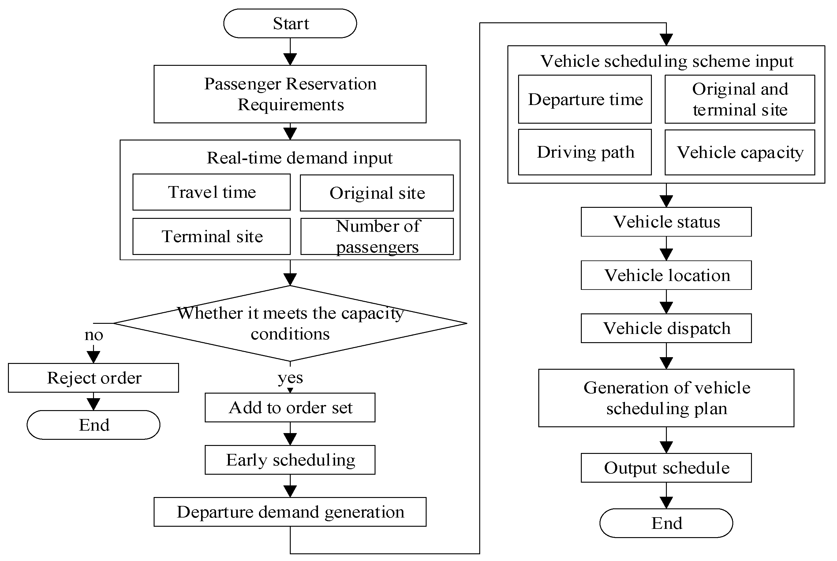
3.1.1. Real-Time Scheduling Process of Demand-Responsive Buses
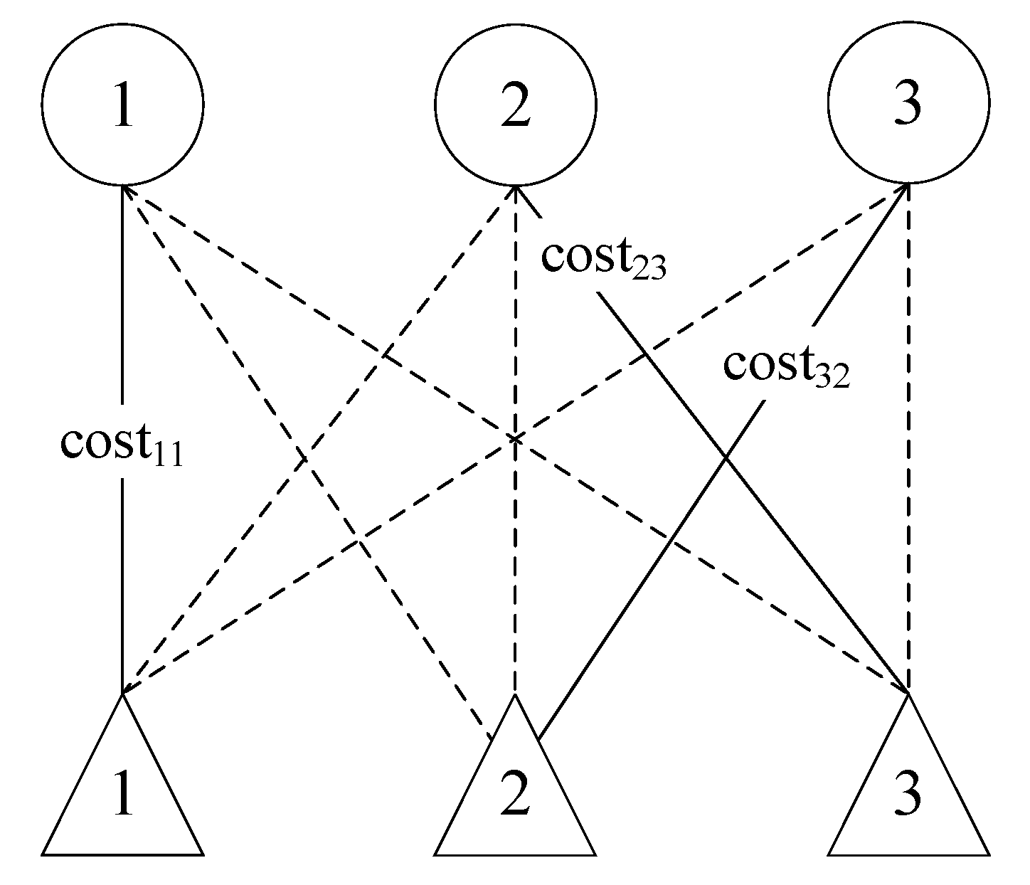
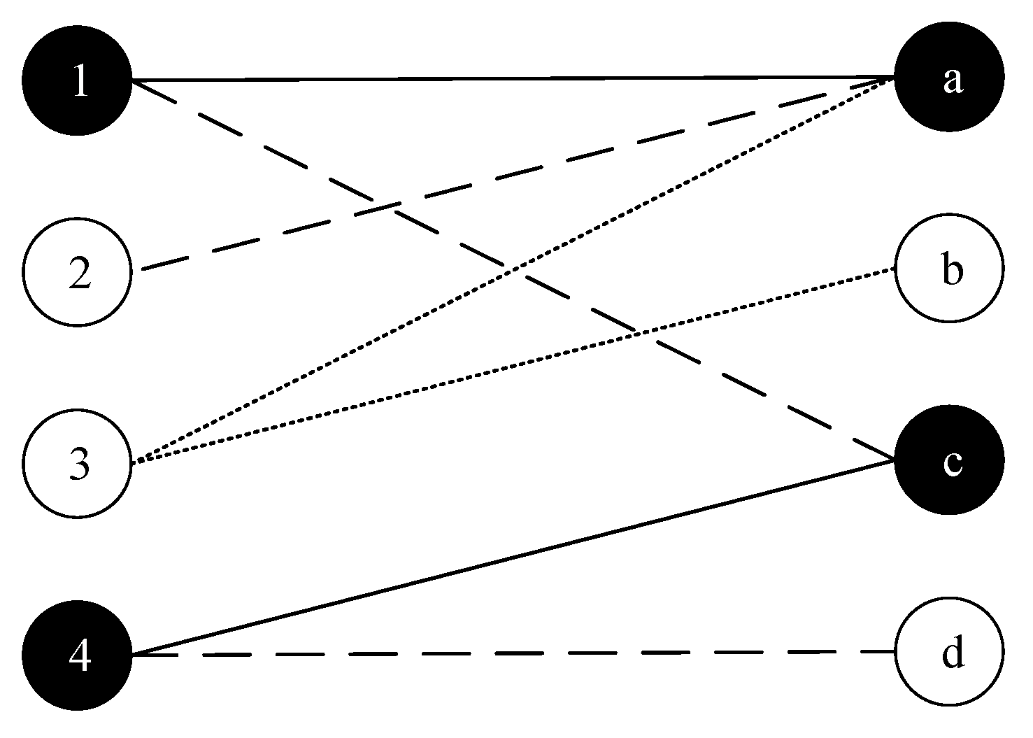
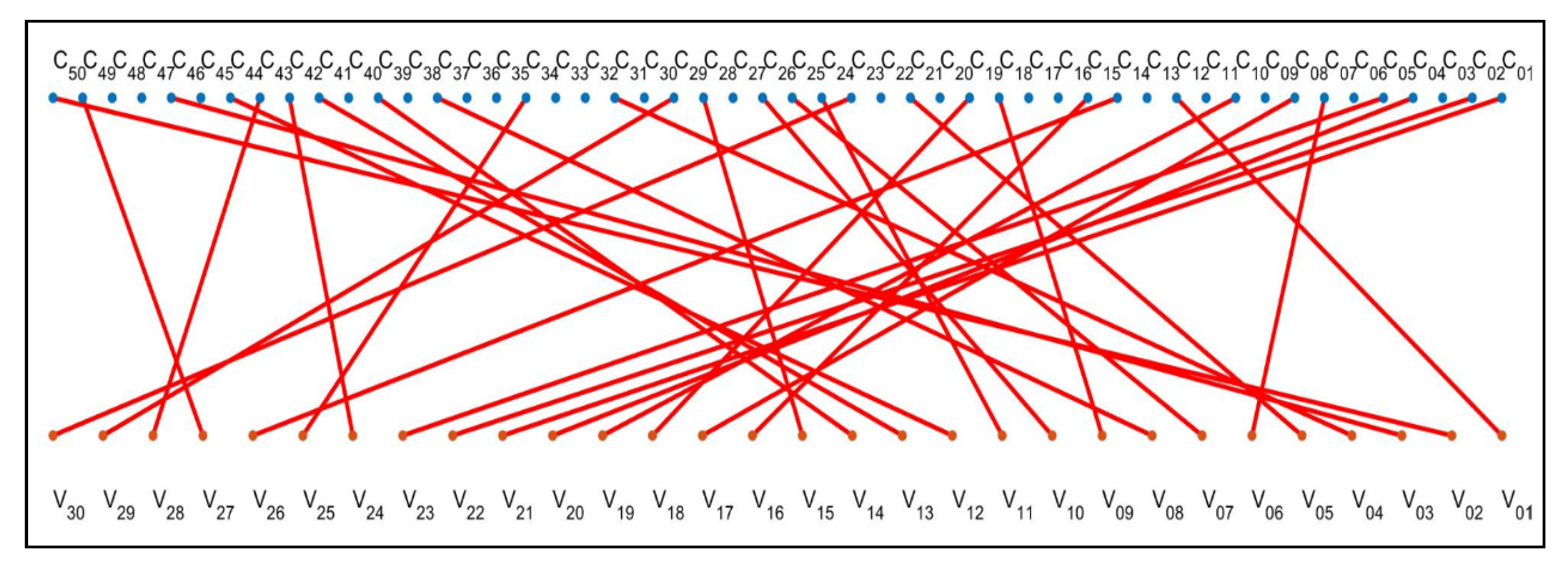
3.1.2. Problem Description Based on Weighted Bipartite Graph
3.2. Assumptions and Parameter Descriptions
3.2.1. Assumptions
- (1)
- Before vehicle dispatching, the task of the next departure time is known, including the departure time, departure station, final arrival station, and required vehicle type;
- (2)
- The vehicles are all dispatched by the dispatch center, and the model, location information, and passenger status of each vehicle are known;
- (3)
- Different types of vehicles have the same basic conditions except for the different passenger capacities;
- (4)
- The driving distance between each station is known;
- (5)
- To ensure the service level of the system, it is necessary to ensure that the number of vehicles of each model in the system is sufficient;
- (6)
- After the previous task of the vehicle is over, it stays at the terminal of the previous task and waits for dispatch;
- (7)
- During the actual operation, the vehicle is allowed to turn around;
- (8)
- The impact on vehicle dispatch due to emergencies and other reasons will not be considered for the time being.
3.2.2. Parameter Descriptions
3.3. Mathematical Model Building
3.4. Principle of Optimal Matching and Kuhn–Munkres Algorithm
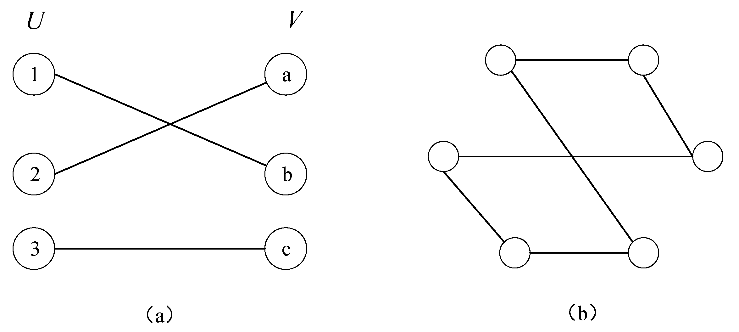
3.4.1. Overview of the Optimal Matching Problem
3.4.2. Optimal Matching Theory
- (1)
- Maximum matching
- It has the largest number of matching edges;
- There may be many different matching methods, but the maximum number of matching sides is the same and certain;
- It cannot have more than half the number of edges than the number of vertices in the graph.
- (2)
- Weighted maximum matching
- (3)
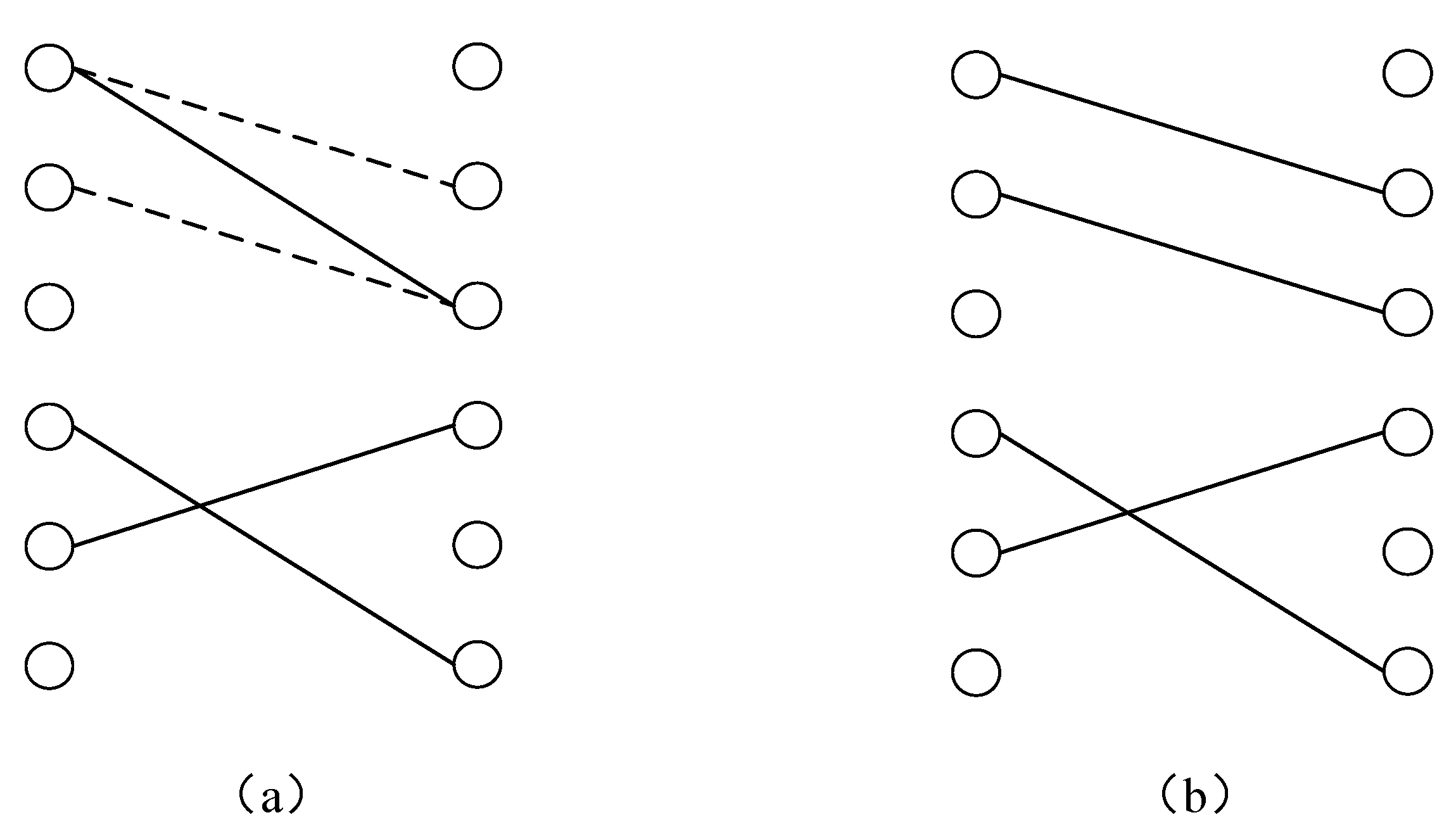
- Alternating path
- (4)
- Augmenting path
3.4.3. Basic Principles of the Kuhn–Munkres Algorithm
3.4.4. Solution Process
4. Case Studies
4.1. Introduction to Calculation Examples
4.2. Generation of Vehicle Tasks Based on Real-Time Demand
4.3. Result Analysis
5. Conclusions
Author Contributions
Funding
Institutional Review Board Statement
Informed Consent Statement
Data Availability Statement
Acknowledgments
Conflicts of Interest
References
- Nie, Q.; Zhang, L.; Tong, Z.; Hubacek, K. Strategies for applying carbon trading to the new energy vehicle market in China: An improved evolutionary game analysis for the bus industry. Energy 2022, 259, 124904. [Google Scholar] [CrossRef]
- Huang, D.; Tong, W.; Wang, L.; Yang, X. An analytical model for the many-to-one demand responsive transit systems. Sustainability 2019, 12, 298. [Google Scholar] [CrossRef] [Green Version]
- Saxena, N.; Rashidi, T.; Rey, D. Determining the market uptake of demand responsive transport enabled public transport service. Sustainability 2020, 12, 4914. [Google Scholar] [CrossRef]
- Wang, Y.; Zhang, D.; Hu, L.; Yang, Y.; Lee, L.H. A data-driven and optimal bus scheduling model with time-dependent traffic and demand. IEEE Trans. Intell. Transp. Syst. 2017, 18, 2443–2452. [Google Scholar] [CrossRef]
- Perumal, S.S.G.; Lusby, R.M.; Larsen, J. Electric bus planning & scheduling: A review of related problems and methodologies. Eur. J. Oper. Res. 2022, 301, 395–413. [Google Scholar]
- Zhou, X.; Xi, J.; Guan, Z.; Ji, X. Dispatching Design for Customized Bus of Hybrid Vehicles Based on Reservation Data. J. Adv. Transp. 2021, 2021, 8868291. [Google Scholar] [CrossRef]
- Dakic, I.; Yang, K.; Menendez, M.; Chow, J.Y.J. On the design of an optimal flexible bus dispatching system with modular bus units: Using the three-dimensional macroscopic fundamental diagram. Transp. Res. Part B Methodol. 2021, 148, 38–59. [Google Scholar] [CrossRef]
- Sadrani, M.; Tirachini, A.; Antoniou, C. Vehicle dispatching plan for minimizing passenger waiting time in a corridor with buses of different sizes: Model formulation and solution approaches. Eur. J. Oper. Res. 2022, 299, 263–282. [Google Scholar] [CrossRef]
- Yan, X.; Zhao, X.; Han, Y.; Van Hentenryck, P.; Dillahunt, T. Mobility-on-demand versus fixed-route transit systems: An evaluation of traveler preferences in low-income communities. Transp. Res. Part A Policy Pract. 2021, 148, 481–495. [Google Scholar] [CrossRef]
- Liu, T.; Ceder, A.A. Analysis of a new public-transport-service concept: Customized bus in China. Transp. Policy 2015, 39, 63–76. [Google Scholar] [CrossRef]
- Li, J.; He, Z.; Zhong, J. The Multi-Type Demands Oriented Framework for Flex-Route Transit Design. Sustainability 2022, 14, 9727. [Google Scholar] [CrossRef]
- Guo, R.; Guan, W.; Zhang, W. Route design problem of customized buses: Mixed integer programming model and case study. J. Transp. Eng. Part A Syst. 2018, 144, 04018069. [Google Scholar] [CrossRef]
- Zhang, J.; Li, W.; Wang, G.; Yu, J. Feasibility Study of Transferring Shared Bicycle Users with Commuting Demand to Flex-Route Transit—A Case Study of Nanjing City, China. Sustainability 2021, 13, 6067. [Google Scholar] [CrossRef]
- Daganzo, C.F. Checkpoint dial-a-ride systems. Transp. Res. Part B 1984, 18, 315–327. [Google Scholar] [CrossRef]
- Cortés, C.E.; Jayakrishnan, R. Design and Operational Concepts of High-Coverage Point-to-Point Transit System. Transp. Res. Record 2002, 1783, 178–187. [Google Scholar] [CrossRef]
- Wang, H.; Li, J.; Wang, P.; Teng, J.; Loo, B.P.Y. Adaptability analysis methods of demand responsive transit: A review and future directions. Transp. Rev. 2023, 1–22. [Google Scholar] [CrossRef]
- Kim, M.E.; Schonfeld, P. Maximizing net benefits for conventional and flexible bus services. Transp. Res. Part A 2015, 80, 116–133. [Google Scholar] [CrossRef]
- Fang, Y.; Hu, X.; Wu, L.; Miao, Y. A Real-Time Scheduling Method for a Variable-Route Bus in a Community[C]//Advances in Intelligent Decision Technologies: Proceedings of the Second KES International Symposium IDT 2010; Springer: Berlin/Heidelberg, Germany, 2010; pp. 239–247. [Google Scholar]
- Kim, M.E.; Levy, J.; Schonfeld, P. Optimal zone sizes and headways for flexible-route bus services. Transp. Res. Part B Methodol. 2019, 130, 67–81. [Google Scholar]
- Schofer, J.L.; Nelson, B.L.; Eash, R.; Daskin, M.; Wan, Y.; Yan, J.; Medgyesy, L. Resource Requirements for Demand-Responsive Transportation Services. In Transportation Research Board; 2003; Available online: https://books.google.co.kr/books?hl=zh-CN&lr=&id=RG9wnNBKCy4C&oi=fnd&pg=PA1&dq=Resource+Requirements+for+Demand-Responsive+Transportation+Services&ots=vFhed40Vrg&sig=BH2eRBLY3xfUA514V41LRlfWuC4&redir_esc=y#v=onepage&q=Resource%20Requirements%20for%20Demand-Responsive%20Transportation%20Services&f=false (accessed on 12 February 2023).
- Qiu, F.; Li, W.; Zhang, J. A dynamic station strategy to improve the performance of flex-route transit services. Transp. Res. Part C 2014, 48, 229–240. [Google Scholar] [CrossRef]
- Gorev, A.; Popova, O.; Solodkij, A. Demand-responsive transit systems in areas with low transport demand of “smart city”. Transp. Res. Procedia 2020, 50, 160–166. [Google Scholar] [CrossRef]
- Mulley, C.; Nelson, J.; Teal, R.; Wright, S.; Daniels, R. Barriers to implementing flexible transport services: An international comparison of the experiences in Australia, Europe and USA. Res. Transp. Bus. Manag. 2012, 3, 3–11. [Google Scholar] [CrossRef]
- Errico, F.; Crainic, T.G.; Malucelli, F.; Nonato, M. A survey on planning semi-flexible transit systems: Methodological issues and a unifying framework. Transp. Res. Part C 2013, 36, 324–338. [Google Scholar] [CrossRef]
- Diana, M.; Dessouky, M.M.; Xia, N. A model for the fleet sizing of demand responsive transportation services with time windows. Transp. Res. Part B Methodol. 2006, 40, 651–666. [Google Scholar] [CrossRef] [Green Version]
- Yao, E.; Liu, T.; Lu, T.; Yang, Y. Optimization of electric vehicle scheduling with multiple vehicle types in public transport. Sustain. Cities Soc. 2020, 52, 101862. [Google Scholar] [CrossRef]
- Bie, Y.; Tang, R.; Wang, L. Bus scheduling of overlapping routes with multi-vehicle types based on passenger OD data. IEEE Access 2019, 8, 1406–1415. [Google Scholar] [CrossRef]
- Hu, B.; Fu, Y.; Feng, S. Integrated optimization of multi-vehicle-type timetabling and scheduling to accommodate periodic passenger flow. In Computer-Aided Civil and Infrastructure Engineering; Wiley: Online, 2023. [Google Scholar]
- Guedes, P.C.; Borenstein, D. Real-time multi-depot vehicle type rescheduling problem. Transp. Res. Part B Methodol. 2018, 108, 217–234. [Google Scholar] [CrossRef]


| Symbol | Symbol Description |
|---|---|
| Determine the departure time | |
| The task of the vehicle numbered m | |
| Idle vehicle numbered n | |
| Collection of sites | |
| The starting site of the vehicle task m | |
| Terminal of vehicle number m | |
| Initial station where the idle vehicle n is located | |
| The distance between the starting station of the vehicle task m and the initial station of the vehicle n | |
| The starting and ending distance of the vehicle task m | |
| The vehicle n to move to the starting station of the vehicle task m when it is empty | |
| Average vehicle speed | |
| Vehicle types, respectively representing small-sized bus, Medium-sized bus, and large-sized bus | |
| The vehicle type required for the task m, | |
| Vehicle n, | |
| K -type vehicle unit distance running cost of an empty vehicle, that is, the cost of empty driving | |
| K -type vehicle unit distance carrying passenger operating cost | |
| Maximum transfer time allowed | |
| Decision variable, whether the vehicle task m matches the vehicle n |
| Station Number | Station Name | Coordinates (m) |
|---|---|---|
| 01 | Zhaoxian Road, Huyi Highway | 0 |
| 02 | Hongde Road, Huyi Highway | 587 |
| 03 | Baiyin Road, Huyi Highway | 1117 |
| 04 | Shigang | 1683 |
| 05 | Yining Road, Huyi Highway | 2215 |
| 06 | Huyi Highway Hope Road | 2696 |
| 07 | Shuangdan Road, Huyi Highway | 3336 |
| 08 | Malu Town | 3896 |
| 09 | Huyi Highway Baoan Highway | 4540 |
| 10 | Yagang Road, Huyi Highway | 5393 |
| 11 | Daqiaotou | 7093 |
| 12 | Chenxiang Road, Huyi Highway | 7745 |
| Vehicle | Number of Seats | Vehicle Type | Fixed Cost | Passenger Operating Cost | Empty Operation Cost |
|---|---|---|---|---|---|
| 2020 SAIC Roewe Ei5 | 5 seats | Small-sized bus | 36 CNY/vehicle | 1.35 CNY/km | 1.30 CNY/km |
| 2021 Maxus EV90 | 15 seats | Medium-sized bus | 40 CNY/vehicle | 1.9 CNY/km | 1.85 CNY/km |
| Yancheng Brand HYK6700YBEV | 23 seats | Large-sized bus | 55 CNY/vehicle | 2.1 CNY/km | 2.05 CNY/km |
| Task Number | Starting Station | Terminal Station | Required Vehicle |
|---|---|---|---|
| 1 | Hongde Road, Huyi Highway | Malu Town | Large-sized bus |
| 2 | Baiyin Road, Huyi Highway | Shigang | Small-sized bus |
| 3 | Zhaoxian Road, Huyi Highway | Shuangdan Road, Huyi Highway | Medium-sized bus |
| 4 | Yagang Road, Huyi Highway | Huyi Highway Baoan Highway | Large-sized bus |
| 5 | Shuangdan Road, Huyi Highway | Yagang Road, Huyi Highway | Medium-sized bus |
| 6 | Chenxiang Road, Huyi Highway | Baiyin Road, Huyi Highway | Medium-sized bus |
| 7 | Malu Town | Baiyin Road, Huyi Highway | Large-sized bus |
| 8 | Baiyin Road, Huyi Highway | Daqiaotou | Large-sized bus |
| 9 | Zhaoxian Road, Huyi Highway | Baiyin Road, Huyi Highway | Small-sized bus |
| 10 | Yagang Road, Huyi Highway | Huyi Highway Hope Road | Large-sized bus |
| 11 | Huyi Highway Hope Road | Hongde Road, Huyi Highway | Small-sized bus |
| 12 | Shigang | Huyi Highway Baoan Highway | Small-sized bus |
| 13 | Zhaoxian Road, Huyi Highway | Huyi Highway Baoan Highway | Small-sized bus |
| 14 | Malu Town | Shigang | Medium-sized bus |
| 15 | Shuangdan Road, Huyi Highway | Zhaoxian Road, Huyi Highway | Medium-sized bus |
| 16 | Hongde Road, Huyi Highway | Yagang Road, Huyi Highway | Medium-sized bus |
| 17 | Daqiaotou | Daqiaotou | Small-sized bus |
| 18 | Daqiaotou | Yining Road, Huyi Highway | Large-sized bus |
| 19 | Huyi Highway Hope Road | Zhaoxian Road, Huyi Highway | Large-sized bus |
| 20 | Huyi Highway Hope Road | Shuangdan Road, Huyi Highway | Large-sized bus |
| 21 | Baiyin Road, Huyi Highway | Daqiaotou | Large-sized bus |
| 22 | Zhaoxian Road, Huyi Highway | Baiyin Road, Huyi Highway | Small-sized bus |
| 23 | Huyi Highway Baoan Highway | Hongde Road, Huyi Highway | Medium-sized bus |
| 24 | Shigang | Malu Town | Small-sized bus |
| 25 | Baiyin Road, Huyi Highway | Huyi Highway Baoan Highway | Small-sized bus |
| 26 | Huyi Highway Hope Road | Baiyin Road, Huyi Highway | Medium-sized bus |
| 27 | Huyi Highway Baoan Highway | Huyi Highway Hope Road | Medium-sized bus |
| 28 | Shigang | Hongde Road, Huyi Highway | Large-sized bus |
| 29 | Daqiaotou | Hongde Road, Huyi Highway | Medium-sized bus |
| 30 | Shuangdan Road, Huyi Highway | Shuangdan Road, Huyi Highway | Small-sized bus |
| Vehicle Type | Quantity |
|---|---|
| Small-sized bus | 13 |
| Medium-sized bus | 20 |
| Large-sized bus | 17 |
| Task Number | KM Algorithm Matching Scheme | Greedy Algorithm Matching Scheme | ||
|---|---|---|---|---|
| Vehicle Number | Type of Vehicle | Vehicle Number | Type of Vehicle | |
| 1 | 12 | Large-sized bus | 12 | Large-sized bus |
| 2 | 50 | Large-sized bus | 34 | Small-sized bus |
| 3 | 46 | Medium-sized bus | 2 | Medium-sized bus |
| 4 | 31 | Large-sized bus | 26 | Large-sized bus |
| 5 | 21 | Large-sized bus | 39 | Medium-sized bus |
| 6 | 7 | Medium-sized bus | 7 | Medium-sized bus |
| 7 | 25 | Large-sized bus | 19 | Large-sized bus |
| 8 | 37 | Large-sized bus | 1 | Large-sized bus |
| 9 | 18 | Medium-sized bus | 41 | Small-sized bus |
| 10 | 26 | Large-sized bus | 31 | Large-sized bus |
| 11 | 24 | Small-sized bus | 42 | Small-sized bus |
| 12 | 44 | Small-sized bus | 44 | Small-sized bus |
| 13 | 41 | Small-sized bus | 23 | Small-sized bus |
| 14 | 39 | Medium-sized bus | 49 | Medium-sized bus |
| 15 | 28 | Medium-sized bus | 14 | Medium-sized bus |
| 16 | 15 | Medium-sized bus | 15 | Medium-sized bus |
| 17 | 8 | Small-sized bus | 8 | Small-sized bus |
| 18 | 19 | Large-sized bus | 25 | Large-sized bus |
| 19 | 10 | Large-sized bus | 4 | Large-sized bus |
| 20 | 4 | Large-sized bus | 10 | Large-sized bus |
| 21 | 1 | Large-sized bus | 37 | Large-sized bus |
| 22 | 2 | Medium-sized bus | 24 | Small-sized bus |
| 23 | 5 | Medium-sized bus | 5 | Medium-sized bus |
| 24 | 42 | Small-sized bus | 33 | Small-sized bus |
| 25 | 34 | Small-sized bus | 13 | Small-sized bus |
| 26 | 14 | Medium-sized bus | 28 | Medium-sized bus |
| 27 | 49 | Medium-sized bus | 45 | Medium-sized bus |
| 28 | 43 | Large-sized bus | 43 | Large-sized bus |
| 29 | 29 | Medium-sized bus | 29 | Medium-sized bus |
| 30 | 23 | Small-sized bus | 17 | Small-sized bus |
| Total operating cost (CNY) | 177.67 | 195.34 | ||
Disclaimer/Publisher’s Note: The statements, opinions and data contained in all publications are solely those of the individual author(s) and contributor(s) and not of MDPI and/or the editor(s). MDPI and/or the editor(s) disclaim responsibility for any injury to people or property resulting from any ideas, methods, instructions or products referred to in the content. |
© 2023 by the authors. Licensee MDPI, Basel, Switzerland. This article is an open access article distributed under the terms and conditions of the Creative Commons Attribution (CC BY) license (https://creativecommons.org/licenses/by/4.0/).
Share and Cite
Zhou, X.; Wei, G.; Zhang, Y.; Wang, Q.; Guo, H. Optimizing Multi-Vehicle Demand-Responsive Bus Dispatching: A Real-Time Reservation-Based Approach. Sustainability 2023, 15, 5909. https://doi.org/10.3390/su15075909
Zhou X, Wei G, Zhang Y, Wang Q, Guo H. Optimizing Multi-Vehicle Demand-Responsive Bus Dispatching: A Real-Time Reservation-Based Approach. Sustainability. 2023; 15(7):5909. https://doi.org/10.3390/su15075909
Chicago/Turabian StyleZhou, Xuemei, Guohui Wei, Yunbo Zhang, Qianlin Wang, and Huanwu Guo. 2023. "Optimizing Multi-Vehicle Demand-Responsive Bus Dispatching: A Real-Time Reservation-Based Approach" Sustainability 15, no. 7: 5909. https://doi.org/10.3390/su15075909