
Projections of Beach Erosion and Associated Costs in Chile
 , ,
, ,
Abstract
:1. Introduction
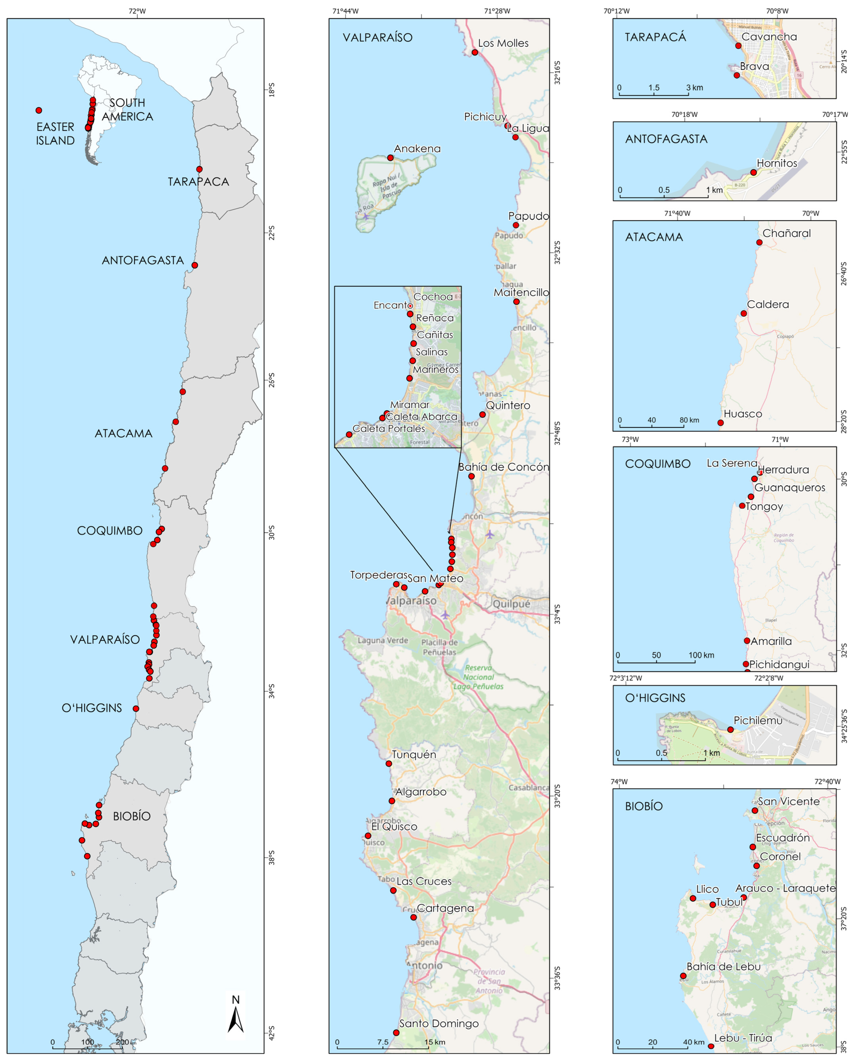
2. Study Sites
3. Methodology
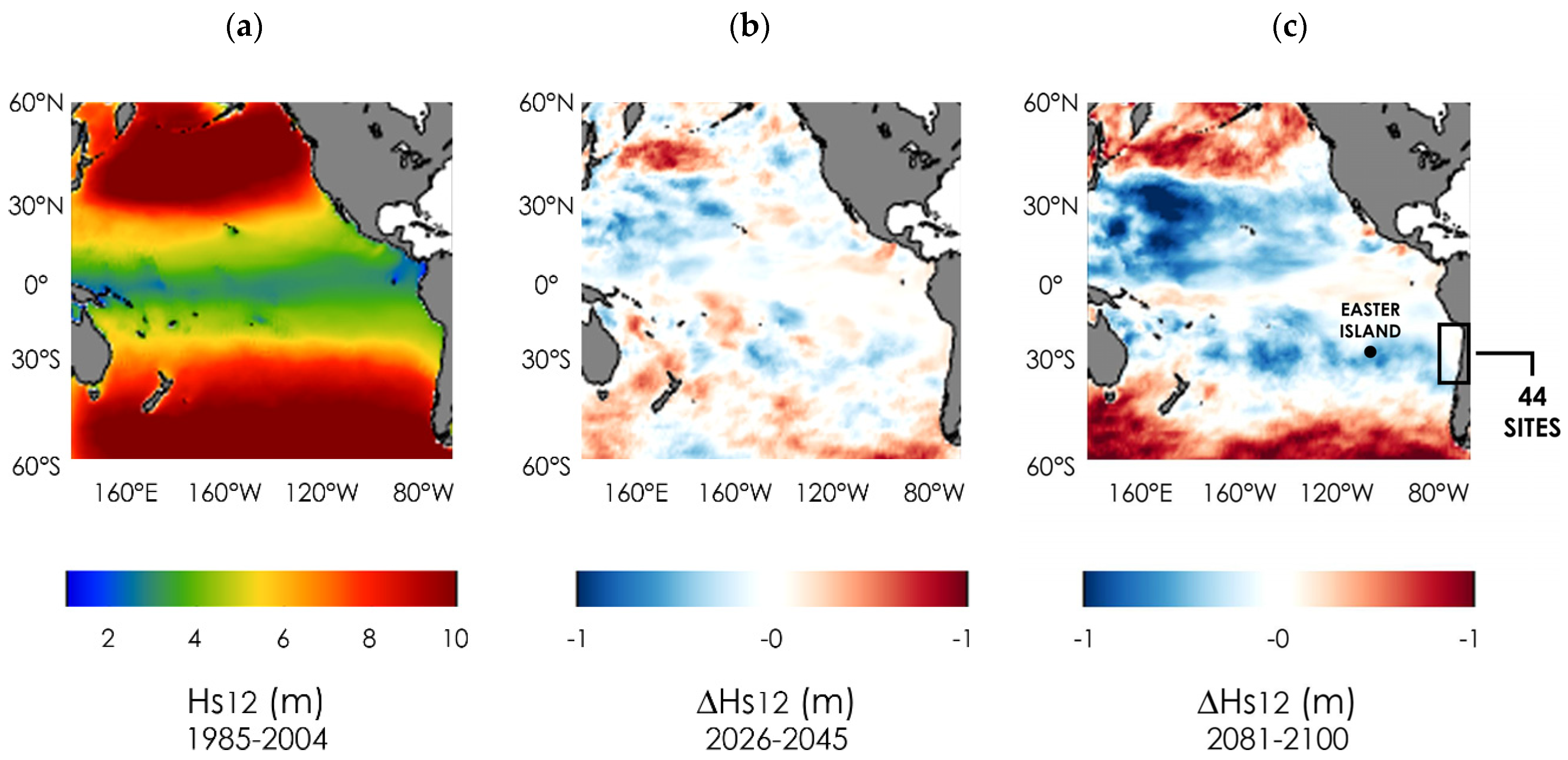
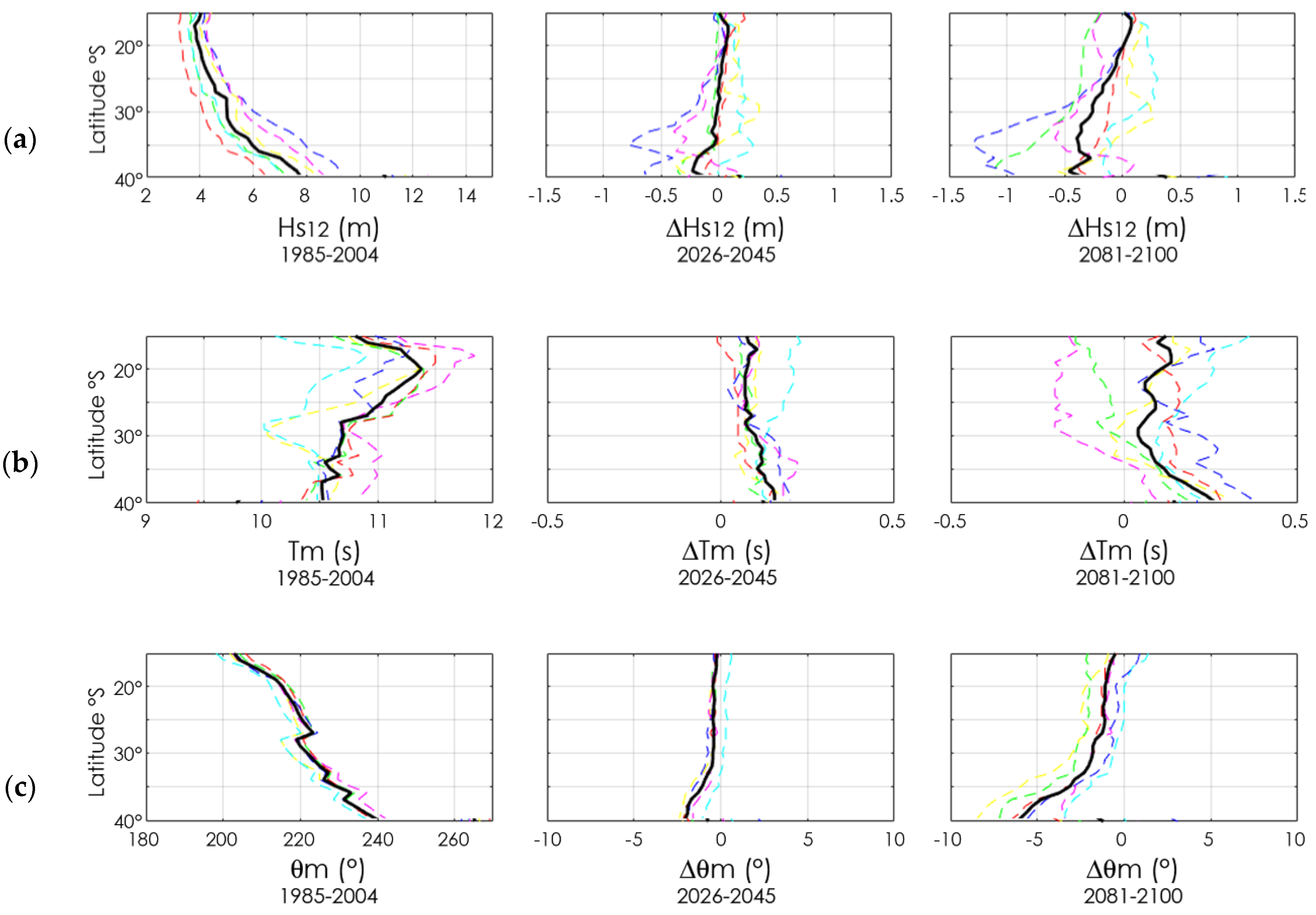
3.1. Projections of Wave Climate
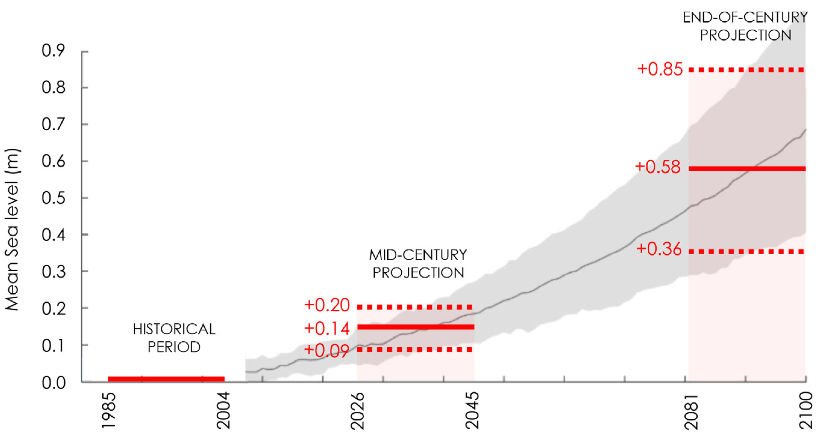
3.2. Projections Sea-Level Rise
3.3. Projections of Shoreline Change
3.4. Projections of Economic Losses Due to Beach Erosion
4. Results
4.1. Projections of Wave Climate
4.2. Projections Sea-Level Rise
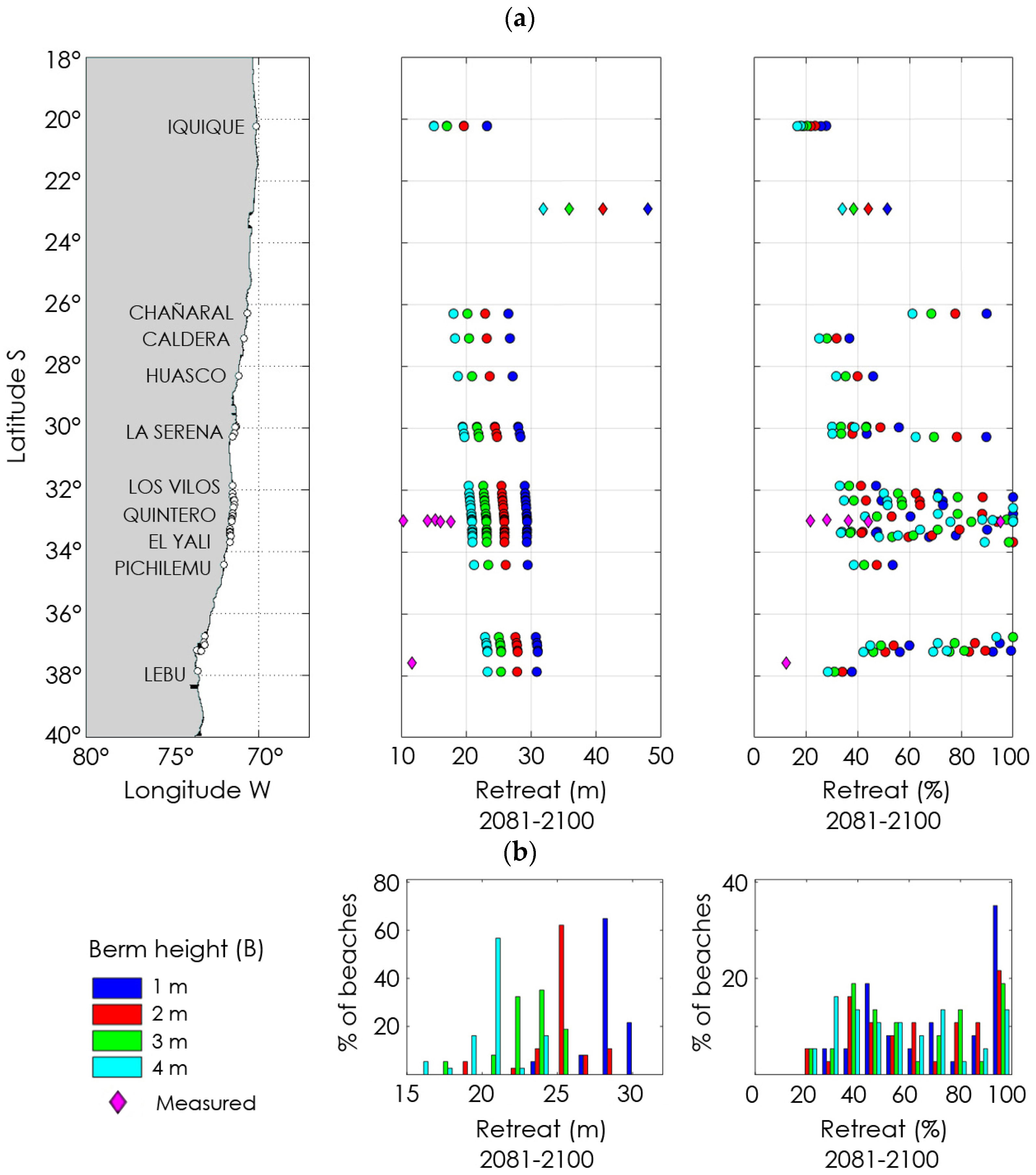
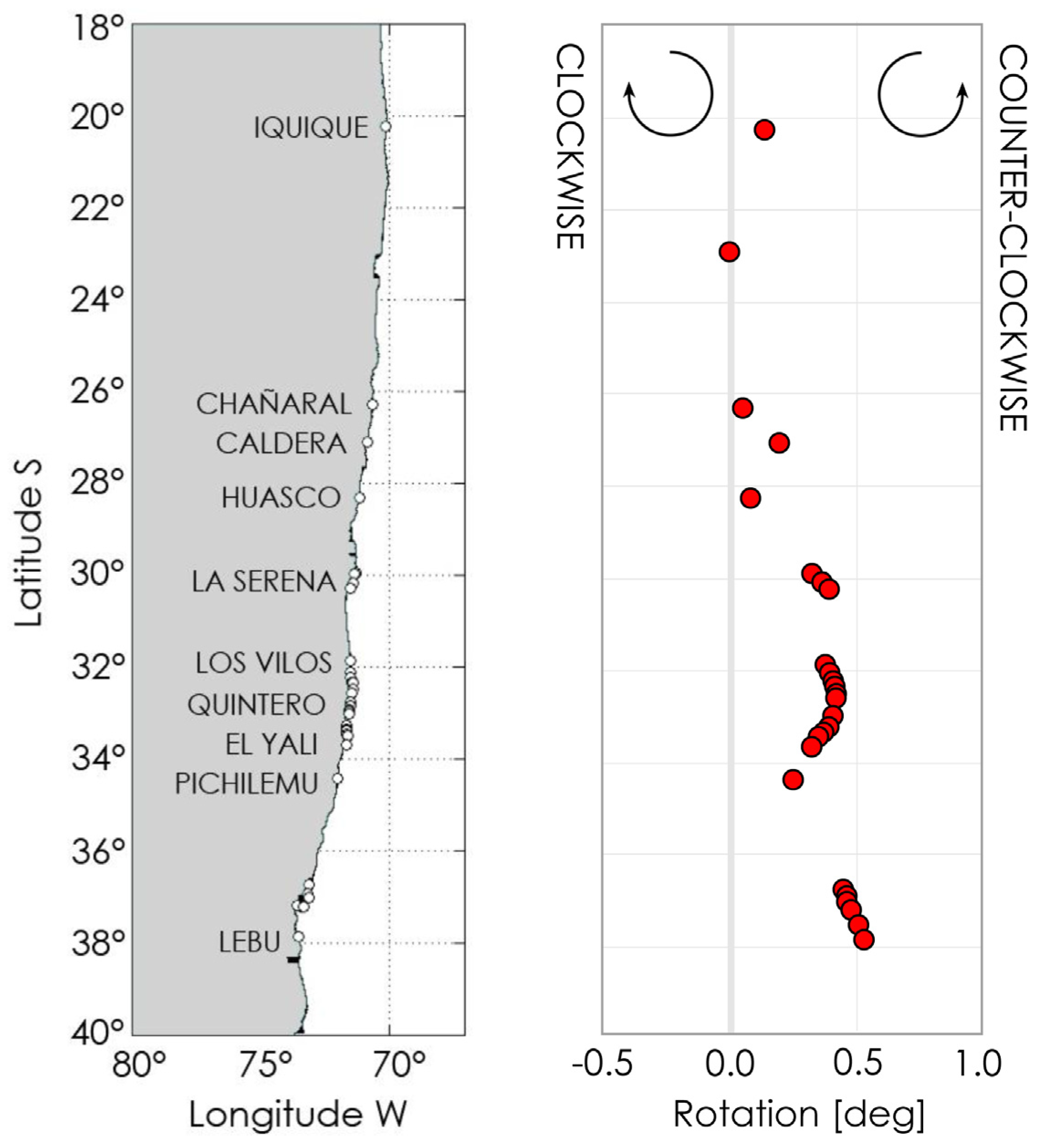
4.3. Projections of Shoreline Change
4.4. Projections of Economic Losses Due to Beach Erosion
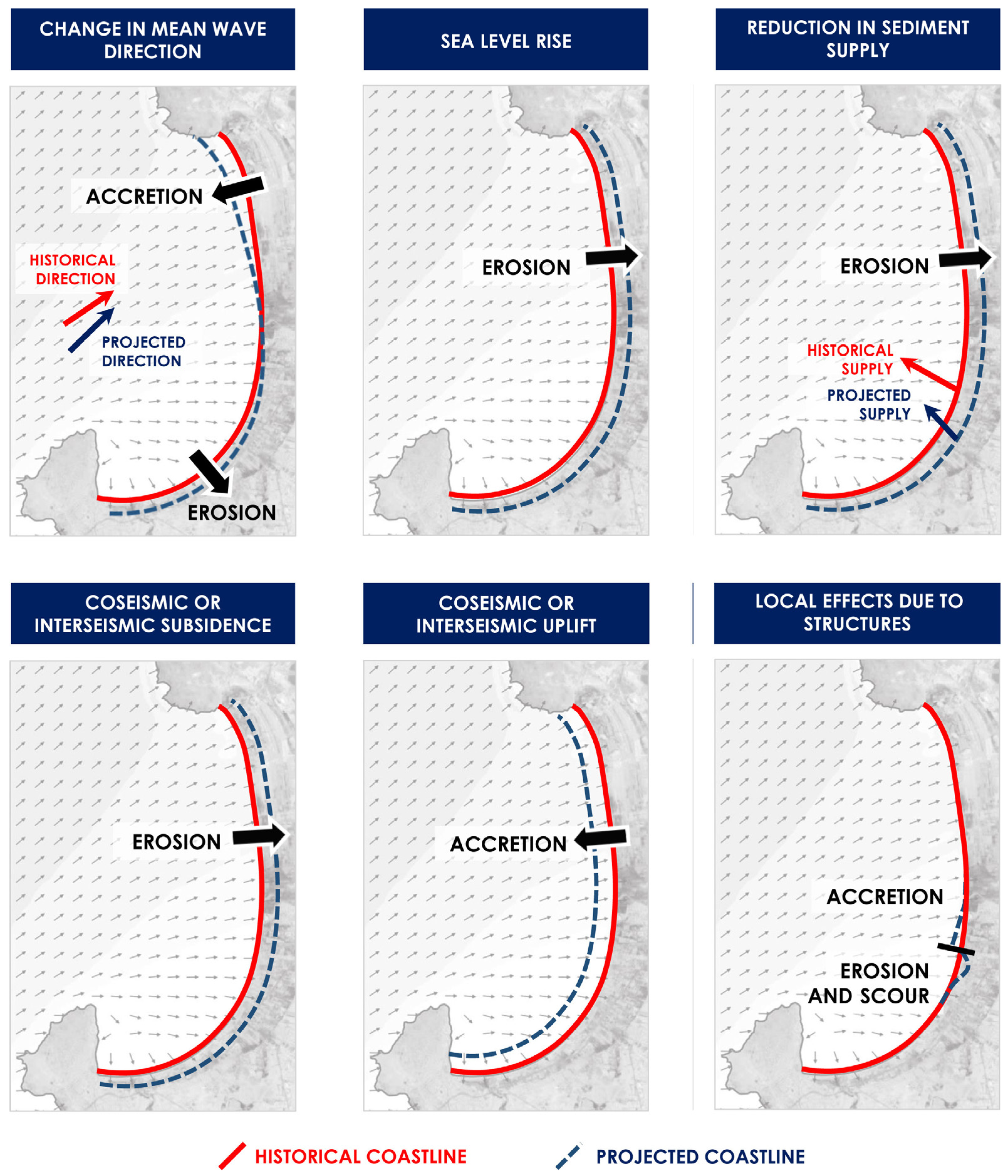
5. Discussion
5.1. Projections of Shoreline Change
5.2. Projections of Economic Losses Due to Beach Erosion
6. Conclusions
Supplementary Materials
Author Contributions
Funding
Informed Consent Statement
Acknowledgments
Conflicts of Interest
References
- Ranasinghe, R.; Stive, M. Rising seas and retreating coastlines. Clim. Chang. 2009, 97, 465–468. [Google Scholar] [CrossRef] [Green Version]
- Chust, A.; Caballero, A.; Marcos, M.; Liria, P.; Hernández, C.; Borja, A. Regional scenarios of sea level rise and impacts on Basque (Bay of Biscay) coastal habitats, throughout the 21st century. Estuar. Coast. Shelf Sci. 2010, 87, 113–124. [Google Scholar] [CrossRef] [Green Version]
- Masselink, G.; Castelle, B.; Scott, T.; Dodet, G.; Suanez, S.; Jackson, D.; Floc’h, F. Extreme wave activity during 2013/2014 winter and morphological impacts along the Atlantic coast of Europe. Geophys. Res. Lett. 2016, 43, 2135–2143. [Google Scholar] [CrossRef]
- Uyarra, M.C.; Cote, I.M.; Gill, J.A.; Tinch, R.R.; Viner, D.; Watkinson, A.R. Islands pecific preferences of tourists for environmental features: Implications of climate change for tourism-dependent states. Environ. Conserv. 2005, 32, 11–19. [Google Scholar] [CrossRef] [Green Version]
- Bird, E.C. World-wide trends in sandy shoreline changes during the past century. Géographie Phys. Et Quat. 2011, 35, 241–244. [Google Scholar] [CrossRef] [Green Version]
- Vitousek, S.; Barnard, P.; Limber, P. Can beaches survive climate change? J. Geophys. Res. Earth Surf. 2017, 122, 1060–1067. [Google Scholar] [CrossRef]
- Luijendijk, A.; Hagenaars, G.; Ranasinghe, R.; Baart, F.; Donchyts, G.; Aarninkhof, S. The State of the World’s Beaches. Sci. Rep. 2018, 8, 6641. [Google Scholar] [CrossRef]
- Vousdoukas, M.; Ranasinghe, R.; Mentaschi, L.; Plomaritis, T.; Athanasiou, P.; Luijendijk, A.; Feyen, L. Sandy coastlines under threat of erosion. Nat. Clim. Chang. 2020, 10, 260–263. [Google Scholar] [CrossRef]
- Cooper, A.; Masselink, G.; Coco, G.; Short, A.; Castelle, B.; Rogers, K.; Anthony, E.; Green, A.; Kelly, J.; Pilkey, O.; et al. Sandy beaches can survive sea-level rise. Nat. Clim. Chang. 2020, 10, 993–995. [Google Scholar] [CrossRef]
- Bagheri, M.; Zaiton Ibrahim, Z.; Bin Mansor, Z.; Abd Manaf, L.; Badarulzaman, N.; Vaghefi, N. Shoreline change analysis and erosion prediction using historical data of Kuala Terengganu, Malaysia. Environ. Earth Sci. 2019, 78, 477. [Google Scholar] [CrossRef]
- Jiménez, J.; Sancho-García, A.; Bosom, E.; Valdemoro, E.; Guillén, J. Storm-induced damages along the Catalan coast (NW Mediterranean) during the period 1958–2008. Geomorphology 2012, 143–144, 24–33. [Google Scholar] [CrossRef]
- Drius, M.; Bongiorni, L.; Depellegrin, D.; Menegon, S.; Pugnetti, A.; Stifter, S. Tackling challenges for Mediterranean sustainable coastal tourism: An ecosystem service perspective. Sci. Total Environ. 2019, 652, 1302–1317. [Google Scholar] [CrossRef]
- Silvestri, F. The Impact of Coastal Erosion on Tourism: A Theoretical Model. Theor. Econ. Lett. 2018, 8, 806–813. [Google Scholar] [CrossRef] [Green Version]
- Manning, R.E.; Lawson, S.R. Carrying capacity as “informed judgment”: The values of science and the science of values. Environ. Manag. 2002, 30, 157–168. [Google Scholar] [CrossRef] [PubMed]
- Jennings, S. Coastal Tourism and Shoreline Management. Ann. Tour. Res. 2004, 31, 899–922. [Google Scholar] [CrossRef]
- Botero, C.; Hurtado, Y. Tourist Beach Sorts as a classification tool for Integrated Beach Management in Latin America. EUCC—Die Küsten Union Dtschl. e.V. 2009, 13, 133–142. [Google Scholar]
- Botero, C.; Noguera, L.; Zielinski, S. Selección por recurrencia de los parámetros de calidad ambiental y turística de los esquemas de certificación de playas en América Latina. Rev. Intrópica 2012, 7, 59–68. [Google Scholar]
- Zielinski, S.; Botero, C. Are eco-labels sustainable? Beach certification schemes in Latin America and the Caribbean. J. Sustain. Tour. 2015, 23, 1550–1572. [Google Scholar] [CrossRef]
- Dragani, W.; Bacinob, G.; Alonso, G. Variation of population density on a beach: A simple analytical formulation. Ocean Coast. Manag. 2021, 208, 105589. [Google Scholar] [CrossRef]
- Nelson, C.; Botterill, D. Evaluating the contribution of beach quality awards to the local tourism industry in Wales—The Green Coast Award. Ocean Coast. Manag. 2002, 45, 157–170. [Google Scholar] [CrossRef]
- Williams, A.; Rangel-Buitrago, N.; Anfuso, G.; Cervantes, O.; Botero, C. Litter impacts on scenery and tourism on the Colombian north Caribbean coast. Tour. Manag. 2016, 55, 209–224. [Google Scholar] [CrossRef]
- Anfuso, G.; Williams, A.; Casas Martínez, G.; Botero, C.; Cabrera Hernández, J.; Pranzini, E. Evaluation of the scenic value of 100 beaches in Cuba: Implications for coastal tourism management. Ocean Coast. Manag. 2018, 142, 173–185. [Google Scholar] [CrossRef]
- De Paula, D.; Lima, J.; Barros, E.; De Santos, J. Coastal Erosion and Tourism: The case of the distribution of tourist accommodations and their daily rates. Geogr. Environ. Sustain. 2021, 14, 110–120. [Google Scholar] [CrossRef]
- Spencer, N.; Strobl, E.; Campbell, A. Sea level rise under climate change: Implications for beach tourism in the Caribbean. Ocean Coast. Manag. 2022, 225, 106207. [Google Scholar] [CrossRef]
- Ruiz-Ramírez, J.D.; Euán-Ávila, J.I.; Rivera-Monroy, V.H. Vulnerability of Coastal Resort Cities to Mean Sea Level Rise in the Mexican Caribbean. Coast. Manag. 2019, 47, 23–43. [Google Scholar] [CrossRef]
- Duan, P.; Cao, Y.; Wang, Y.; Yinet, P. Bibliometric Analysis of Coastal and Marine Tourism Research from 1990 to 2020. J. Coast. Res. 2022, 38, 229–240. [Google Scholar] [CrossRef]
- Łabuz, T.A. Environmental Impacts—Coastal Erosion and Coastline Changes. In Second Assessment of Climate Change for the Baltic Sea Basin; Springer Cham: Cham, Switzerland, 2015; pp. 381–396. [Google Scholar]
- González, S.; Loyola, D.; Yañez-Navea, K. Perception of environmental quality in a beach of high social segregation in northern Chile: Importance of social studies for beach conservation. Ocean Coast. Manag. 2021, 207, 105619. [Google Scholar] [CrossRef]
- Martínez, C.; Winckler, P.; Agredano, R.; Esparza, E.; Torres, I.; Contreras-López, M. Coastal erosion in sandy beaches along a tectonically active coast: The Chile study case. Prog. Phys. Geogr. 2022, 46, 250–271. [Google Scholar] [CrossRef]
- Winckler, P.; Contreras-López, M.; Campos-Caba, R.; Beya, J.; Molina, M. El temporal del 8 de agosto de 2015 en las regiones de Valparaíso y Coquimbo, Chile Central. Lat. Am. J. Aquat. Res. 2017, 45, 622–648. [Google Scholar] [CrossRef]
- Ministerio del Medio Ambiente. Exposición De Zonas Costeras. In Determinación del Riesgo de Los Impactos del Cambio Climático en Las Costas de Chile; Centro UC Cambio Global: Santiago, Chile, 2019; Volume 2. [Google Scholar]
- Araya-Vergara, J. Determinación preliminar de las características del oleaje en Chile Central. Not. Mens. Mus. Nac. Hist. Nat. 1971, 174, 8–12. [Google Scholar]
- Beyá, J.; Álvarez, M.; Gallardo, A.; Hidalgo, H.; Aguirre, C.; Valdivia, J.; Parra, C.; Méndez, L.; Contreras, C.; Winckler, P.; et al. Atlas de Oleaje de Chile; Universidad de Valparaíso: Valparaiso, Chile, 2016; ISBN 978-956-368-194-9. Available online: https://oleaje.uv.cl/descargables/Atlas%20de%20Oleaje%20de%20Chile.pdf (accessed on 1 March 2022).
- Winckler, P.; Aguirre, C.; Farías, L.; Contreras-López, M.; Masotti, I. Evidence of climate-driven changes on atmospheric, hydrological, and oceanographic variables along the Chilean coastal zone. Clim. Chang. 2020, 163, 633–652. [Google Scholar] [CrossRef]
- SHOA. Tablas de Mare de la Costa de Chile. 2009. Available online: http://www.shoa.cl (accessed on 1 March 2022).
- Carvajal, M.; Contreras-Lopez, M.; Winckler, P.; Sepulveda, I. Meteotsunamis Occurring Along the Southwest Coast of South America during an Intense Storm. Pure Appl. Geophys. 2017, 174, 3313–3323. [Google Scholar] [CrossRef]
- González, S.A.; Holtmann-Ahumada, G. Quality of tourist beaches of northern Chile: A first approach for ecosystem-based management. Ocean Coast. Manag. 2017, 137, 154–164. [Google Scholar] [CrossRef]
- Tolman, H.L.; WAVEWATCH III R Development Group. User Manual and System Documentation of WAVEWATCH III °R Version 4.18; Technical Note; Environmental Modeling Center, Marine Modeling and Analysis Branch, NOAA: Washington, DC, USA, 2014. [Google Scholar]
- Taylor, K.E.; Stouffer, R.J.; Meehl, G.A. An Overview of CMIP5 and the experiment design. Bull. Amer. Meteor. Soc. 2012, 93, 485–498. [Google Scholar] [CrossRef] [Green Version]
- Hemer, M.A.; Trenham, C.E. Evaluation of a CMIP5 derived dynamical global wind wave climate model ensemble. Ocean Model. 2016, 103, 190–203. [Google Scholar] [CrossRef] [Green Version]
- WCRP. World Climate Research Programme. Available online: https://esgf-node.llnl.gov/search/cmip5/ (accessed on 1 March 2022).
- NGDC. 2-Minute Gridded Global Relief Data (ETOPO2) v2. National Geophysical Data Center, NOAA. Available online: https://www.ngdc.noaa.gov/mgg/global/etopo2.html (accessed on 1 March 2022).
- Wessel, P.; Smith, W.H. A global, self-consistent, hierarchical, high-resolution shoreline database. J. Geophys. Res. Solid 1996, 101, 8741–8743. [Google Scholar] [CrossRef] [Green Version]
- Ardhuin, F.; Rogers, E.; Babanin, A.; Filipot, J.-F.; Magne, R.; Roland, A.; Van der Westhuysen, A.; Queffeulou, P.; Lefevre, J.-M.; Aouf, L.; et al. Semiempirical dissipation source functions for ocean wave Part I: Definition, calibration and validation. J. Phys. Oceanogr. 2010, 40, 1917–1941. [Google Scholar] [CrossRef] [Green Version]
- Rascle, N.; Ardhuin, F. A global wave parameter database for geophysical applications. Part 2: Model validation with improved source term parameterization. Ocean Model. 2013, 70, 174–188. [Google Scholar] [CrossRef] [Green Version]
- Hasselmann, S.; Hasselmann, K.; Allender, J.; Barnett, T. Computatuons and parameterizations of the nonlinear energy transfer in gravity-wave spectrum, part II: Parameterizations of the nonlinear energy transfer for application in wave models. J. Phys. Oceanogr. 1985, 15, 1378–1392. [Google Scholar] [CrossRef]
- Beyá, J.; Álvarez, M.; Gallardo, A.; Hidalgo, H.; Winckler, P. Generation and validation of the Chilean Wave Atlas database. Ocean Model. 2017, 116, 16–32. [Google Scholar] [CrossRef]
- Winckler, P.; Contreras-López, M.; Garreaud, R.; Meza, F.; Larraguibel, C.; Esparza, C.; Gelcich, S.; Falvey, M.; Mora, J. Analysis of Climate-Related Risks for Chile’s Coastal Settlements in the ARClim Web Platform. Water 2022, 14, 3594. [Google Scholar] [CrossRef]
- Booij, N.; Holthuijsen, L.H.; Ris, R.C. The “SWAN” Wave Model for Shallow Water. In Coastal Engineering; OJS/PKP: Phoenix, AZ, USA, 1996; pp. 668–676. [Google Scholar]
- Massel, S. Ocean Surface Waves: Their Physics and Prediction; Advanced Series on Ocean Engineering; World Scientific: Singapore, 1996; Volume 11. [Google Scholar]
- Lemos, G.; Menendez, M.; Semedo, A.; Camus, P.; Hemer, M.; Dobrynin, M.; Miranda, P.M. On the need of bias correction methods for wave climate projections. Glob. Planet. Chang. 2020, 186, 103109. [Google Scholar] [CrossRef]
- Saha, S.; Moorthi, S.; Pan, H.L.; Wu, X.; Wang, J.; Nadiga, S.; Tripp, P.; Kistler, R.; Woollen, J.; Behringer, D.; et al. The NCEP climate forecast system reanalysis. Bull. Amer. Meteor. 2010, 91, 1015–1058. [Google Scholar] [CrossRef] [Green Version]
- Dalrymple, R.A.; Dean, R.G. Water Wave Mechanics for Engineers and Scientists; Advanced Series on Ocean Engineering; World Scientific: Singapore, 1991; Volume 2. [Google Scholar]
- Church, J.A.; Clark, P.U.; Cazenave, A.; Gregory, J.M.; Jevrejeva, S.; Levermann, A.; Merrifield, M.A.; Milne, G.A.; Nerem, R.S.; Nunn, P.D.; et al. Chapter 13—Sea Level Change. In Climate Change 2013: The Physical Science Basis; Contribution of Working Group I to the Fifth Assessment Report of the Intergovernmental Panel on Climate Change; Cambridge University Press: New York, NY, USA, 2013; Volume 13, pp. 1137–1216. [Google Scholar]
- Slangen, A.B.A.; Carson, M.; Katsman, C.A.; Van de Wal, R.S.W.; Köhl, A.; Vermeersen, L.L.A.; Stammer, D. Projecting twenty-first century regional sea-level changes. Clim. Chang. 2014, 124, 317–332. [Google Scholar] [CrossRef]
- Short, A.D.; Masselink, G. Embayed and Structurally Controlled Beaches. In Handbook of Beach and Shoreface Morphodynamics; Short, A.D., Ed.; John Wiley: Chichester, UK, 1999; pp. 230–249. [Google Scholar]
- Bruun, P. Sea-level rise as a cause of shore erosion. J. Waterw. Harb. Div. 1962, 88, 117–130. [Google Scholar] [CrossRef]
- Birkemeier, W.A. Field data on seaward limit of profile change. J. Waterw. Port Coast. Ocean Eng. 1985, 111, 598–602. [Google Scholar] [CrossRef] [Green Version]
- Dean, R.G. Coastal Sediment Processes: Toward Engineering Solutions. In Coastal Sediments ’87, Proceedings of a Specialty Conference on Advances in Understanding of Coastal Sediment Processes, New Orleans, LA, USA, 12–14 May 1987; American Society of Civil Engineers: New York, NY, USA, 1987. [Google Scholar]
- Enriquez-Acevedo, T.; Botero, C.M.; Cantero-Rodelo, R.; Pertuz, A.; Suarez, A. Willingness to pay for Beach Ecosystem Services: The case study of three Colombian beaches. Ocean Coast. Manag. 2018, 161, 96–104. [Google Scholar] [CrossRef]
- Raheem, N.; Colt, S.; Fleishman, E.; Talberth, J.; Swedeen, P.; Boyle, K.J.; Rudd, M.; Lopez, R.D.; Crocker, D.; Bohan, D.; et al. Application of non-market valuation to California’s coastal policy decisions. Mar. Policy 2012, 36, 1166–1171. [Google Scholar] [CrossRef]
- Landry, C.E.; Keeler, A.G.; Kriesel, W. An economic evaluation of beach erosion management alternatives. Mar. Resour. Econ. 2003, 18, 105–127. [Google Scholar] [CrossRef]
- Landry, C.E.; Hindsley, P. Valuing beach quality with hedonic property models. Land Econ. 2011, 87, 92–108. [Google Scholar] [CrossRef]
- Gopalakrishnan, S.; Smith, M.D.; Slott, J.M.; Murray, A.B. The value of disappearing beaches: A hedonic pricing model with endogenous beach width. J. Environ. Econ. Manag. 2011, 61, 297–310. [Google Scholar] [CrossRef] [Green Version]
- Parsons, G.R.; Chen, Z.; Hidrue, M.K.; Standing, N.; Lilley, J. Valuing Beach Width for Recreational Use: Combining Revealed and Stated Preference Data. Mar. Resour. Econ. 2013, 28, 221–241. [Google Scholar] [CrossRef]
- Huang, J.C.; Poor, P.J.; Zhao, M.Q. Economic valuation of beach erosion control. Mar. Resour. Econ. 2007, 22, 221–238. [Google Scholar] [CrossRef]
- Desvousges, W.H.; Naughton, M.C.; Parsons, G.R. Benefit transfer: Conceptual problems in estimating water quality benefits using existing studies. Water Resour. Res. 1992, 28, 675–683. [Google Scholar] [CrossRef] [Green Version]
- Johnston, R.J.; Ramachandran, M.; Parsons, G.R. Benefit Transfer Combining Revealed and Stated Preference Data. In Benefit Transfer of Environmental and Resource Values; Springer Dordrecht: Dordrecht, The Netherlands, 2015; pp. 163–189. [Google Scholar]
- Servicio Nacional de Turismo (SERNATUR). Encuesta Nacional de Viajes de los Residentes de Chile. 2018. Available online: http://www.subturismo.gob.cl/turismo-interno/ (accessed on 18 December 2020).
- Lucero, F.; Catalán, P.A.; Ossandón, A.; Beyá, J.; Puelma, A.; Zamorano, L. Wave energy assessment in the central-south coast of Chile. Renew. Energ. 2017, 114, 120–131. [Google Scholar] [CrossRef]
- Aguirre, C.; García-Loyola, S.; Testa, G.; Silva, D.; Farias, L. Insight into anthropogenic forcing on coastal upwelling off south-central Chile. Elem. Sci. Anth. 2018, 6, 59. [Google Scholar] [CrossRef]
- Rykaczewski, R.R.; Dunne, J.P.; Sydeman, W.J.; García-Reyes, M.; Black, B.A.; Bograd, S.J. Poleward displacement of coastal upwelling-favorable winds in the ocean’s eastern boundary currents through the 21st century. Geophys. Res. Lett. 2015, 42, 6424–6431. [Google Scholar] [CrossRef]
- Sierra, J.P.; Casas-Prat, M. Analysis of potential impacts on coastal areas due to changes in wave conditions. Clim. Chang. 2014, 124, 861–876. [Google Scholar] [CrossRef] [Green Version]
- Ranasinghe, R. Assessing climate change impacts on open sandy coasts: A review. Earth Sci. Rev. 2016, 160, 320–332. [Google Scholar] [CrossRef] [Green Version]
- Winckler, P.; Esparza, C.; Mora, J.; Agredano, R.; Contreras-López, M.; Larraguibel, C.; Melo, O.; Contreras.López, M. Impactos del Cambio Climático en Las Costas de Chile. In Hacia una Ley de Costas en Chile: Bases Para una Gestión Integrada de Áreas Litorales; Martínez, C., Arenas, F., Bergamini, K., Urrea, J., Eds.; Serie GEOlibro N°38, Instituto de Geografía, Pontificia Universidad Católica de Chile: Santiago, Chile, 2022. [Google Scholar]
- Albrecht, F.; Shaffer, G. Regional Sea-Level Change along the Chilean Coast in the 21st Century. J. Coast. Res. 2016, 32, 1322–1332. [Google Scholar] [CrossRef]
- Rangel-Buitrago, N.; Anfuso, G.; Williams, A. Coastal erosion problems along the Caribbean Coast of Colombia. Ocean Coast. Manag. 2015, 114, 120–144. [Google Scholar] [CrossRef]
- Cai, F.; Su, X.; Liu, J.; Li, B.; Lei, G. Coastal erosion in China under the condition of global climate change and measures for its prevention. Prog. Nat. Sci. 2009, 19, 415–426. [Google Scholar] [CrossRef]
- Fritz, H.M.; Petroff, C.M.; Catalán, P.A.; Cienfuegos, R.; Winckler, P.; Kalligeris, N.; Weiss, R.; Barrientos, S.E.; Meneses, G.; Valderas-Bermejo, C.; et al. Field survey of the 27 February 2010 Chile tsunami. Pure Appl. Geophys. 2011, 168, 1989–2010. [Google Scholar] [CrossRef]
- Poulos, A.; Monsalve, M.; Zamora, N.; de la Llera, J.C. An Updated Recurrence Model for Chilean Subduction Seismicity and Statistical Validation of Its Poisson Nature. Bull. Seismol. Soc. Am. 2019, 109, 66–74. [Google Scholar] [CrossRef]
- Schurr, B.; Asch, G.; Rosenau, M.; Wang, R.; Oncken, O.; Barrientos, S.; Vilotte, J.P. The 2007 M7.7 Tocopilla Northern Chile Earthquake Sequence: Implications for Along-strike and Downdip Rupture Segmentation and Megathrust Frictional Behavior. J. Geophys. Res. Solid. 2012, 117, 1–19. [Google Scholar] [CrossRef] [Green Version]
- Sepúlveda, I.; Haase, J.; Liu, P.L.-F.; Grigoriu, M.; Winckler, P. Non-stationary Probabilistic Tsunami Hazard Assessments Incorporating Climate-change-driven Sea Level Rise and Application to South China Sea. Earth’s Future 2021, 9, e2021EF002007. [Google Scholar] [CrossRef]
- Cooper, J.A.G.; Pilkey, O.H. Sea-level rise and shoreline retreat: Time to abandon the Bruun Rule. Glob. Planet. Chang. 2004, 43, 157–171. [Google Scholar] [CrossRef]
- Rosati, J.D.; Dean, R.G.; Walton, T.L. The modified Bruun Rule extended for landward transport. Mar. Geol. 2013, 340, 71–81. [Google Scholar] [CrossRef] [Green Version]
- Toimil, A.; Losada, I.J.; Camus, P.; Diaz-Simal, P. Managing coastal erosion under climate change at the regional scale. Coast. Eng. 2017, 128, 106–122. [Google Scholar] [CrossRef]
- Toimil, A.; Camus, P.; Losada, I.J.; Le Cozannet, G.; Nicholls, R.J.; Idier, D.; Maspataud, A. Climate change-driven coastal erosion modelling in temperate sandy beaches: Methods and uncertainty treatment. Earth Sci. Rev. 2020, 202, 103110. [Google Scholar] [CrossRef]


| # | Beach | Lat (° S) | Lon (° W) | Type | Shape | Length (m) | Width (m) | Area (m2) | Orientation (° N) | ||
|---|---|---|---|---|---|---|---|---|---|---|---|
| 1 | Cavancha | 20.23 | 70.15 | U | Embayed | 940 | 56–110 | ✘ | ✘ | 78,020 | 240° |
| 2 | Brava | 20.24 | 70.15 | U | Rectilinear | 2795 | 62–117 | ✘ | ✘ | 250,153 | 80° |
| 3 | Hornitos | 22.92 | 70.29 | R | Embayed | 6400 | 39–147 | 0.12 | ✘ | 595,200 | 281° |
| 4 | Chañaral | 26.30 | 70.65 | U | Embayed | 5147 | 24–35 | ✘ | ✘ | 151,837 | 220° |
| 5 | Caldera | 27.10 | 70.86 | U, PU | Embayed | 6181 | 47–98 | ✘ | ✘ | 448,123 | 300° |
| 6 | Huasco | 28.33 | 71.17 | R | Embayed | 3570 | 44–74 | ✘ | ✘ | 210,630 | 275° |
| 7 | La Serena | 29.96 | 71.32 | U | Embayed | 18,850 | 44–108 | ✘ | ✘ | 1,214,620 | 266°–330° |
| 8 | La Herradura | 29.98 | 71.36 | U | Embayed | 1574 | 26–95 | ✘ | ✘ | 78,800 | 325° |
| 9 | Guanaqueros | 30.29 | 71.53 | U, PU | Embayed | 5900 | 25–86 | ✘ | ✘ | 382,596 | 325° |
| 10 | Tongoy | 30.19 | 71.40 | U | Embayed | 11,630 | 28–32 | ✘ | ✘ | 367,625 | 337° |
| 11 | Los Vilos | 31.87 | 71.50 | PU | Embayed | 2780 | 53–70 | ✘ | ✘ | 170,970 | 65° |
| 12 | Pichidangui | 32.12 | 71.51 | PU | Embayed | 2996 | 20–61 | ✘ | ✘ | 122,252 | 315° |
| 13 | Los Molles | 32.24 | 71.51 | PU | Embayed | 1460 | 20–80 | ✘ | ✘ | 42,245 | 199° |
| 14 | Pichicuy | 32.34 | 71.45 | PU | Embayed | 2184 | 10–120 | ✘ | ✘ | 129,128 | 228° |
| 15 | La Ligua | 32.36 | 71.43 | PU | Embayed | 5800 | 30–50 | ✘ | ✘ | 232,000 | 230° |
| 16 | Papudo | 32.49 | 71.43 | U | Embayed | 2129 | 30–50 | ✘ | ✘ | 85,160 | 310° |
| 17 | Maitencillo | 32.59 | 71.45 | U | Embayed | 224 | 13–25 | ✘ | ✘ | 3483 | 335° |
| 18 | Quintero | 32.78 | 71.50 | I | Embayed | 7360 | 13–85 | ✘ | ✘ | 215,458 | 252°–340° |
| 19 | Concón | 32.86 | 71.51 | R, PU | Rectilinear | 10,392 | 10–132 | ✘ | ✘ | 504,547 | 264°–270° |
| 20 | Cochoa | 32.96 | 71.55 | U | Embayed | 160 | 11–46 | ✘ | ✘ | 3214 | 315° |
| 21 | El Encanto | 32.96 | 71.55 | U | Rectilinear | 232 | 9–26 | ✘ | ✘ | 5494 | 257° |
| 22 | Reñaca | 32.97 | 71.55 | U | Rectilinear | 1300 | 20–70 | 0.50 | 3.54 | 70,488 | 264° |
| 23 | Las Cañitas | 32.98 | 71.55 | PU | Embayed | 185 | 13–28 | ✘ | ✘ | 4193 | 275° |
| 24 | Las Salinas | 32.99 | 71.55 | U | Embayed | 190 | 20–40 | 0.63 | 2.74 | 7324 | 290° |
| 25 | Los Marineros | 33.00 | 71.55 | U | Rectilinear | 2680 | 25–68 | 0.75 | 4.54 | 125,889 | 278°–300° |
| 26 | Miramar | 33.02 | 71.57 | U | Embayed | 147 | 14–21 | ✘ | ✘ | 1517 | 325° |
| 27 | Caleta Abarca | 33.02 | 71.57 | U | Rectilinear | 420 | 18–33 | ✘ | ✘ | 11,570 | 312° |
| 28 | Caleta Portales | 33.03 | 71.59 | U | Rectilinear | 633 | 0–83 | 0.42 | 3.37 | 11,718 | 330° |
| 29 | Torpederas | 33.02 | 71.64 | U | Embayed | 95 | 38–38 | 0.50 | 3.00 | 3460 | 333° |
| 30 | Tunquén | 33.29 | 71.66 | R | Embayed | 2184 | 10–68 | ✘ | ✘ | 71,252 | 241° |
| 31 | Algarrobo | 33.36 | 71.66 | U | Embayed | 2484 | 39–97 | ✘ | ✘ | 153,137 | 275° |
| 32 | El Quisco | 33.39 | 71.69 | U | Embayed | 1050 | 43–107 | ✘ | ✘ | 65,410 | 295° |
| 33 | Las Cruces | 33.47 | 71.65 | PU | Embayed | 376 | 47–53 | ✘ | ✘ | 14,161 | 224° |
| 34 | Cartagena | 33.52 | 71.61 | U, PU | Embayed | 4456 | 10–90 | ✘ | ✘ | 193,372 | 230°–266° |
| 35 | St. Domingo | 33.69 | 71.65 | U, PU | Rectilinear | 21,807 | 10–88 | ✘ | ✘ | 513,612 | 285°–305° |
| 36 | Pichilemu | 34.43 | 72.04 | PU | Embayed | 4201 | 10–90 | ✘ | ✘ | 230,996 | 287°–333° |
| 37 | San Vicente | 36.76 | 73.14 | I, PU | Embayed | 5460 | 6–41 | ✘ | ✘ | 133,622 | 313°–348° |
| 38 | Escuadrón | 36.95 | 73.17 | U, PU | Rectilinear | 8555 | 25–40 | ✘ | ✘ | 278,347 | 286° |
| 39 | Playa Blanca | 37.03 | 73.15 | PU | Embayed | 1790 | 20–107 | ✘ | ✘ | 92,248 | 293° |
| 40 | Tubul | 37.23 | 73.44 | PU | Embayed | 1227 | 9–52 | ✘ | ✘ | 41,250 | 50° |
| 41 | Llico | 37.18 | 73.56 | R | Rectilinear | 2257 | 25–44 | ✘ | ✘ | 70,510 | 25° |
| 42 | Arauco | 37.24 | 73.31 | U, PU | Rectilinear | 12,658 | 49–86 | ✘ | ✘ | 696,862 | 322° |
| 43 | Bahía de Lebu | 37.59 | 73.65 | PU | Embayed | 2862 | 68–126 | ✘ | ✘ | 270,026 | 310° |
| 44 | Lebu–Tirúa | 37.88 | 73.54 | R | Embayed | 4283 | 43–130 | 0.60 | 6.50 | 349,227 | 264° |
| 45 | Anakena | 27.07 | 109.32 | R | Embayed | 241 | 12–40 | ✘ | ✘ | 7273 | 344° |
| Type of Trip | Change in Beach Width | Adjusted WTP (USD) |
|---|---|---|
| Short trip | 1% Decrease | −0.84 |
| 1% Increase | 0.46 | |
| Long trip (more than four nights) | 1% Decrease | −2.07 |
| 1% Increase | 1.14 |
| Beach Reduction | Costs | ||||||
|---|---|---|---|---|---|---|---|
| (%) | Thousands of USD/y | ||||||
| # | Beach | Min | Mean | Max | Min | Mean | Max |
| 1 | Cavancha | 11.1 | 6.7 | 2.2 | 120.0 | 115.2 | 110.3 |
| 2 | Brava | 10.3 | 6.2 | 2.0 | 139.1 | 133.8 | 128.5 |
| 3 | Hornitos | 12.4 | 10.3 | 8.2 | 8.8 | 8.7 | 8.5 |
| 4 | Chañaral | 36.1 | 21.7 | 7.3 | 72.5 | 64.9 | 57.2 |
| 5 | Caldera | 14.9 | 9.0 | 3.0 | 61.2 | 58.0 | 54.9 |
| 6 | Huasco | 18.6 | 11.2 | 3.8 | 9.2 | 8.7 | 8.1 |
| 7 | La Serena | 14.9 | 9.0 | 3.1 | 439.0 | 416.5 | 394.0 |
| 8 | La Herradura | 18.7 | 11.3 | 3.9 | 151.2 | 141.8 | 132.3 |
| 9 | Guanaqueros | 20.6 | 12.4 | 4.3 | 153.6 | 143.2 | 132.9 |
| 10 | Tongoy | 38.3 | 23.1 | 8.0 | 176.1 | 156.8 | 137.5 |
| 11 | Los Vilos | 19.2 | 11.6 | 4.0 | 30.2 | 28.3 | 26.4 |
| 12 | Pichidangui | 29.2 | 17.7 | 6.2 | 32.8 | 29.8 | 26.9 |
| 13 | Los Molles | 23.7 | 14.4 | 5.0 | 37.4 | 34.6 | 31.8 |
| 14 | Pichicuy | 18.2 | 11.1 | 3.9 | 35.8 | 33.6 | 31.4 |
| 15 | La Ligua | 29.7 | 18.0 | 6.3 | 39.2 | 35.7 | 32.2 |
| 16 | Papudo | 29.7 | 18.0 | 6.3 | 219.3 | 199.5 | 179.7 |
| 17 | Maitencillo | 62.6 | 37.9 | 13.3 | 274.9 | 233.2 | 191.5 |
| 18 | Quintero | 24.3 | 14.7 | 5.2 | 210.2 | 194.0 | 177.8 |
| 19 | Concón | 16.8 | 10.2 | 3.6 | 114.4 | 108.0 | 101.5 |
| 20 | Cochoa | 41.9 | 25.4 | 8.9 | 139.0 | 122.9 | 106.7 |
| 21 | El Encanto | 68.2 | 41.3 | 14.5 | 164.8 | 138.5 | 112.2 |
| 22 | Reñaca | 8.4 | 8.4 | 8.4 | 106.2 | 106.2 | 106.2 |
| 23 | Las Cañitas | 58.2 | 35.3 | 12.4 | 155.0 | 132.6 | 110.1 |
| 24 | Las Salinas | 11.6 | 11.6 | 11.6 | 109.3 | 109.3 | 109.3 |
| 25 | Los Marineros | 5.5 | 5.5 | 5.5 | 103.4 | 103.4 | 103.4 |
| 26 | Miramar | 68.2 | 41.4 | 14.6 | 164.8 | 138.6 | 112.3 |
| 27 | Caleta Abarca | 46.8 | 28.4 | 10.0 | 143.9 | 125.8 | 107.8 |
| 28 | Caleta Portales | 10.5 | 10.5 | 10.5 | 108.3 | 108.3 | 108.3 |
| 29 | Torpederas | 10.5 | 10.5 | 10.5 | 108.3 | 108.3 | 108.3 |
| 30 | Tunquén | 30.6 | 18.6 | 6.5 | 351.9 | 319.5 | 287.1 |
| 31 | Algarrobo | 17.5 | 10.6 | 3.8 | 316.7 | 298.1 | 279.5 |
| 32 | El Quisco | 15.9 | 9.7 | 3.4 | 312.3 | 295.5 | 278.6 |
| 33 | Las Cruces | 23.9 | 14.5 | 5.1 | 333.7 | 308.5 | 283.2 |
| 34 | Cartagena | 23.8 | 14.5 | 5.1 | 333.7 | 308.5 | 283.2 |
| 35 | St. Domingo | 24.3 | 14.8 | 5.2 | 334.9 | 309.2 | 283.5 |
| 36 | Pichilemu | 45.5 | 27.7 | 9.8 | 175.5 | 154.0 | 132.5 |
| 37 | San Vicente | 24.6 | 15.0 | 5.5 | 41.9 | 38.7 | 35.5 |
| 38 | Escuadrón | 52.7 | 32.3 | 11.8 | 51.4 | 44.5 | 37.6 |
| 39 | Playa Blanca | 38.2 | 23.4 | 8.6 | 46.5 | 41.5 | 36.5 |
| 40 | Tubul | 19.6 | 12.0 | 4.4 | 27.0 | 25.3 | 23.6 |
| 41 | Llico | 40.8 | 25.0 | 9.1 | 31.8 | 28.3 | 24.7 |
| 42 | Arauco | 36.1 | 22.1 | 8.1 | 30.8 | 27.6 | 24.4 |
| 43 | Bahía de Lebu | 4.3 | 4.3 | 4.3 | 23.6 | 23.6 | 23.6 |
| 44 | Lebu–Tirúa | 12.6 | 7.7 | 2.8 | 25.5 | 24.4 | 23.2 |
| 45 | Anakena | 12.5 | 7.5 | 2.5 | 34.0 | 32.5 | 31.0 |
| Total | 6099 | 5618 | 5136 | ||||
| Beach Reduction | Costs | ||||||
|---|---|---|---|---|---|---|---|
| (%) | Thousands of USD/y | ||||||
| # | Beach | Min | Mean | Max | Min | Mean | Max |
| 1 | Cavancha | 52.0 | 29.5 | 9.1 | 215.8 | 183.9 | 154.8 |
| 2 | Brava | 47.8 | 27.2 | 8.4 | 244.8 | 210.7 | 179.6 |
| 3 | Hornitos | 58.9 | 47.8 | 37.3 | 16.4 | 15.3 | 14.2 |
| 4 | Chañaral | 100.0 | 100.0 | 32.4 | 140.0 | 140.0 | 92.7 |
| 5 | Caldera | 71.6 | 40.3 | 12.8 | 120.2 | 98.2 | 79.0 |
| 6 | Huasco | 93.5 | 51.7 | 16.2 | 19.8 | 15.5 | 11.9 |
| 7 | La Serena | 71.5 | 40.4 | 13.0 | 861.6 | 705.0 | 567.3 |
| 8 | La Herradura | 94.2 | 52.1 | 16.4 | 325.2 | 254.6 | 194.9 |
| 9 | Guanaqueros | 100.0 | 58.0 | 18.1 | 334.9 | 264.5 | 197.8 |
| 10 | Tongoy | 100.0 | 100.0 | 35.1 | 334.9 | 334.9 | 226.1 |
| 11 | Los Vilos | 96.6 | 53.3 | 16.9 | 65.5 | 51.1 | 39.0 |
| 12 | Pichidangui | 100.0 | 87.2 | 26.4 | 66.6 | 62.3 | 42.1 |
| 13 | Los Molles | 100.0 | 68.0 | 21.2 | 79.5 | 66.8 | 48.2 |
| 14 | Pichicuy | 90.7 | 50.4 | 16.2 | 75.8 | 59.8 | 46.2 |
| 15 | La Ligua | 100.0 | 88.8 | 26.9 | 79.5 | 75.1 | 50.5 |
| 16 | Papudo | 100.0 | 89.1 | 27.0 | 444.4 | 420.1 | 282.3 |
| 17 | Maitencillo | 100.0 | 100.0 | 61.6 | 444.4 | 444.4 | 359.1 |
| 18 | Quintero | 100.0 | 70.2 | 21.9 | 444.4 | 378.2 | 271.0 |
| 19 | Concón | 82.1 | 46.1 | 14.9 | 234.5 | 188.1 | 148.0 |
| 20 | Cochoa | 100.0 | 100.0 | 39.4 | 257.6 | 257.6 | 179.6 |
| 21 | El Encanto | 100.0 | 100.0 | 68.4 | 257.6 | 257.6 | 216.9 |
| 22 | Reñaca | 37.0 | 37.0 | 37.0 | 176.4 | 176.4 | 176.4 |
| 23 | Las Cañitas | 100.0 | 100.0 | 57.0 | 257.6 | 257.6 | 202.2 |
| 24 | Las Salinas | 52.8 | 52.8 | 52.8 | 196.8 | 196.8 | 196.8 |
| 25 | Los Marineros | 23.5 | 23.5 | 23.5 | 159.1 | 159.1 | 159.1 |
| 26 | Miramar | 100.0 | 100.0 | 68.6 | 257.6 | 257.6 | 217.1 |
| 27 | Caleta Abarca | 100.0 | 100.0 | 44.7 | 257.6 | 257.6 | 186.3 |
| 28 | Caleta Portales | 47.4 | 47.4 | 47.4 | 189.8 | 189.8 | 189.8 |
| 29 | Torpederas | 47.4 | 47.4 | 47.4 | 189.8 | 189.8 | 189.8 |
| 30 | Tunquén | 100.0 | 92.6 | 28.2 | 708.2 | 682.2 | 453.9 |
| 31 | Algarrobo | 86.6 | 48.4 | 15.7 | 660.8 | 525.5 | 409.7 |
| 32 | El Quisco | 77.0 | 43.4 | 14.2 | 626.7 | 507.8 | 404.3 |
| 33 | Las Cruces | 100.0 | 68.8 | 21.7 | 708.2 | 597.7 | 430.8 |
| 34 | Cartagena | 100.0 | 68.8 | 21.7 | 708.2 | 597.6 | 430.8 |
| 35 | St. Domingo | 100.0 | 70.4 | 22.2 | 708.2 | 603.4 | 432.6 |
| 36 | Pichilemu | 100.0 | 100.0 | 44.4 | 317.2 | 317.2 | 229.0 |
| 37 | San Vicente | 100.0 | 73.0 | 23.8 | 88.4 | 76.5 | 54.7 |
| 38 | Escuadrón | 100.0 | 100.0 | 54.7 | 88.4 | 88.4 | 68.4 |
| 39 | Playa Blanca | 100.0 | 100.0 | 38.2 | 88.4 | 88.4 | 61.1 |
| 40 | Tubul | 100.0 | 56.1 | 18.8 | 59.4 | 46.4 | 35.3 |
| 41 | Llico | 100.0 | 100.0 | 41.2 | 59.4 | 59.4 | 41.9 |
| 42 | Arauco | 100.0 | 100.0 | 36.0 | 59.4 | 59.4 | 40.4 |
| 43 | Bahía de Lebu | 27.4 | 27.4 | 27.4 | 37.9 | 37.9 | 37.9 |
| 44 | Lebu–Tirúa | 60.2 | 34.9 | 12.1 | 47.6 | 40.1 | 33.3 |
| 45 | Anakena | 58.4 | 33.2 | 10.6 | 63.0 | 53.0 | 44.0 |
| Total | 11,778 | 10,549 | 8127 | ||||
Disclaimer/Publisher’s Note: The statements, opinions and data contained in all publications are solely those of the individual author(s) and contributor(s) and not of MDPI and/or the editor(s). MDPI and/or the editor(s) disclaim responsibility for any injury to people or property resulting from any ideas, methods, instructions or products referred to in the content. |
© 2023 by the authors. Licensee MDPI, Basel, Switzerland. This article is an open access article distributed under the terms and conditions of the Creative Commons Attribution (CC BY) license (https://creativecommons.org/licenses/by/4.0/).
Share and Cite
Winckler, P.; Martín, R.A.; Esparza, C.; Melo, O.; Sactic, M.I.; Martínez, C. Projections of Beach Erosion and Associated Costs in Chile. Sustainability 2023, 15, 5883. https://doi.org/10.3390/su15075883
Winckler P, Martín RA, Esparza C, Melo O, Sactic MI, Martínez C. Projections of Beach Erosion and Associated Costs in Chile. Sustainability. 2023; 15(7):5883. https://doi.org/10.3390/su15075883
Chicago/Turabian StyleWinckler, Patricio, Roberto Agredano Martín, César Esparza, Oscar Melo, María Isabel Sactic, and Carolina Martínez. 2023. "Projections of Beach Erosion and Associated Costs in Chile" Sustainability 15, no. 7: 5883. https://doi.org/10.3390/su15075883