Climate and Land-Use Change Impacts on Flood Hazards in the Mono River Catchment of Benin and Togo

Abstract

Flooding is prominent in West Africa, and is expected to be exacerbated, due to global climate and land-use changes. This study assessed the impacts of future climate and land-use changes on flood hazards in the Mono river catchment area of Benin and Togo. Climate scenarios from the representative concentration pathways, RCP 4.5 and RCP 8.5, and land-use projection at the horizon of 2070 were used for runoff simulation at the Athiémé outlet, and flood mapping in the lower Mono river basin. The planned Adjarala dam was also simulated, to evaluate its potential impact. The Soil and Water Assessment Tool (SWAT) was used to investigate the impact of the projected changes on runoff, while the flood-water extent was simulated using the two-dimensional TELEMAC-2D model. TELEMAC-2D was validated with satellite observation and in a participatory way with local stakeholders. SWAT showed good performance during the calibration (KGE = 0.83) and validation (KGE = 0.68) steps. Results show an increase in the magnitude of flood extremes under future climate- and land-use-change scenarios. Events of 10-year return periods during 1987–2010 are expected to become 2-year return-period events under the climate- and land-use-change scenarios considered. The planned Adjarala dam showed potentials for extreme-peak and flood-extent reduction. However, flow-duration curves revealed that the discharge of the river during low-flow periods may also be reduced if the Adjarala dam is built. Adaptation measures as well as sustainable land-use and dam-management options should be identified, to alleviate the impacts of the projected changes.

1. Introduction

The compound effect of climate change and land-use/land-cover change jeopardizes human security around the world [1,2]. It has been established that the trends in precipitation and temperature observed since the 1950s are imputable to human-induced climate change [3]. With a 50% increase in built-up areas, 11.5% increase in croplands, and 2.4% decrease in forest area from 2000 to 2020, the global state of land use and land cover has substantially changed over the past decades [4]. Acting in a feedback loop, changes in land use and climate conditions affect the water cycle, and exacerbate hydrological hazards including floods and droughts [5,6]. Furthermore, the magnitude and frequencies of these events are expected to increase in the coming decades.

However, there are uncertainties about the potential trends and patterns of these hazards in the future. According to the 6th assessment report of the Intergovernmental Panel on Climate Change [7], heavy precipitation and flooding are expected to intensify and be more frequent in most parts of Africa. In addition, the continent is expected, with medium confidence, to experience hydrological droughts. However, extreme precipitation indices in West Africa show mixed patterns, with few statistically significant trends [8]. The projected changes in heavy precipitation over West Africa have low confidence, due to data scarcity and limited evidence [7,9,10]. Moreover, the uncertainty array is further widened with potential uncertainties from climate and hydrological models [11,12]. Therefore, local and regional studies are needed to establish area-specific hazard profiles and to accordingly support decision making.

During the disastrous flood event of 2010 that caused about USD 300 million of loss and damage in Benin and Togo, intense precipitations and the overflow of the Mono river were pointed to, among other causes [13,14]. Recent studies reported the increasing trend in temperature and above-normal precipitation over the past 50 years in the Mono river catchment shared by Benin and Togo [15,16]. In addition, the lower part of the catchment area is prone to higher risks of flooding [17,18]. Extreme precipitation events in the Mono catchment are expected to become more frequent in the future [19,20], despite the ambiguous projected trends [21,22]. Looking to the horizon in 2050, precipitations in the Mono catchment are expected to be characterized by high interannual variabilities, changes in seasons, and a mixture of above- and below-normal precipitations compared to the period 1981–2010 [23,24]. Furthermore, the future land use and land cover (LULC) in the Mono catchment is expected to be characterized by a decrease in forests, and an expansion of settlement and built-up areas [25,26]. Moreover, the two riparian countries intend to build a joint dam, the Adjarala dam, on the Mono river for hydropower energy production, flood protection and for agricultural purposes [27]. However, studies on the potential effect of these climate, land-use, and infrastructural changes on floods in the Mono river basin are lacking. In fact, all the above-mentioned studies addressed either land-use changes or climate trend in the Mono river basin, and not their effect on floods that occur frequently and trigger substantial losses. Questions related to the response of river runoff and flood extent to these changes have so far not been answered in existing works. Therefore, it is important to carry out studies that can incorporate these various types of changes and provide an overview of possible futures with respect to floods in the Mono river basin. Thus, the use of physically based models that can represent the hydrologic and hydrodynamic processes in the basin are needed.

Considering the past and projected changes in the Mono river catchment, this study aims to assess the combined impact of climate and LULC changes, as well as the influence of the forthcoming Adjarala dam on flood hazards in the lower part of the catchment. Climate change data from the representative concentration pathways RCP 4.5 and RCP 8.5, LULC maps and the Adjarala dam information were used for future runoff simulation and, ultimately, for flood mapping. Discharge simulations were performed with the Soil and Water Assessment Tool (SWAT), whereas flood modelling was carried out with the TELEMAC-2D model. The novelty of this study resides in the integrated runoff–flood modeling that was carried out, the assessment of climate and land-use change impacts, and the integration of the planned Adjarala dam into runoff simulation.

2. Materials and Methods

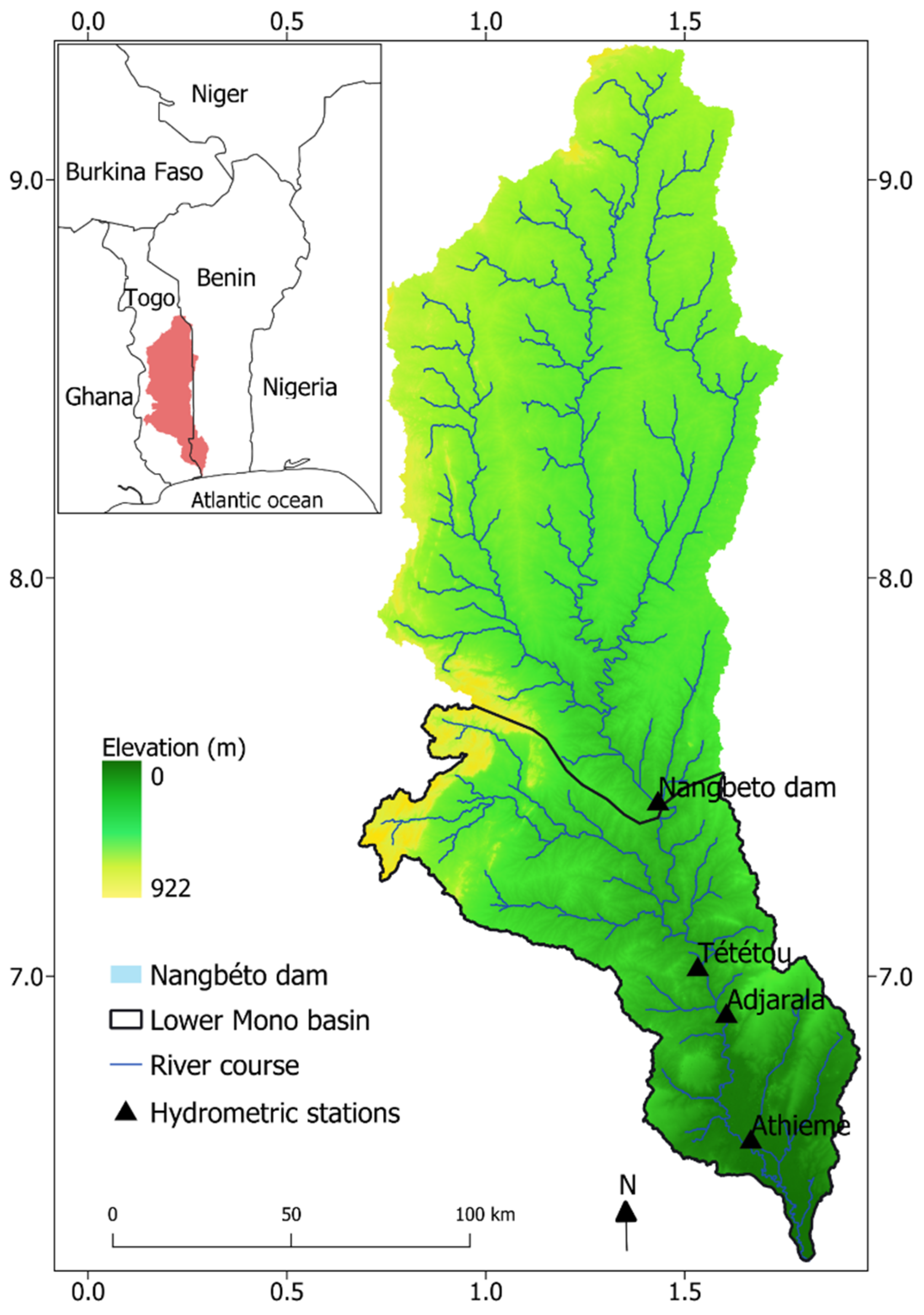
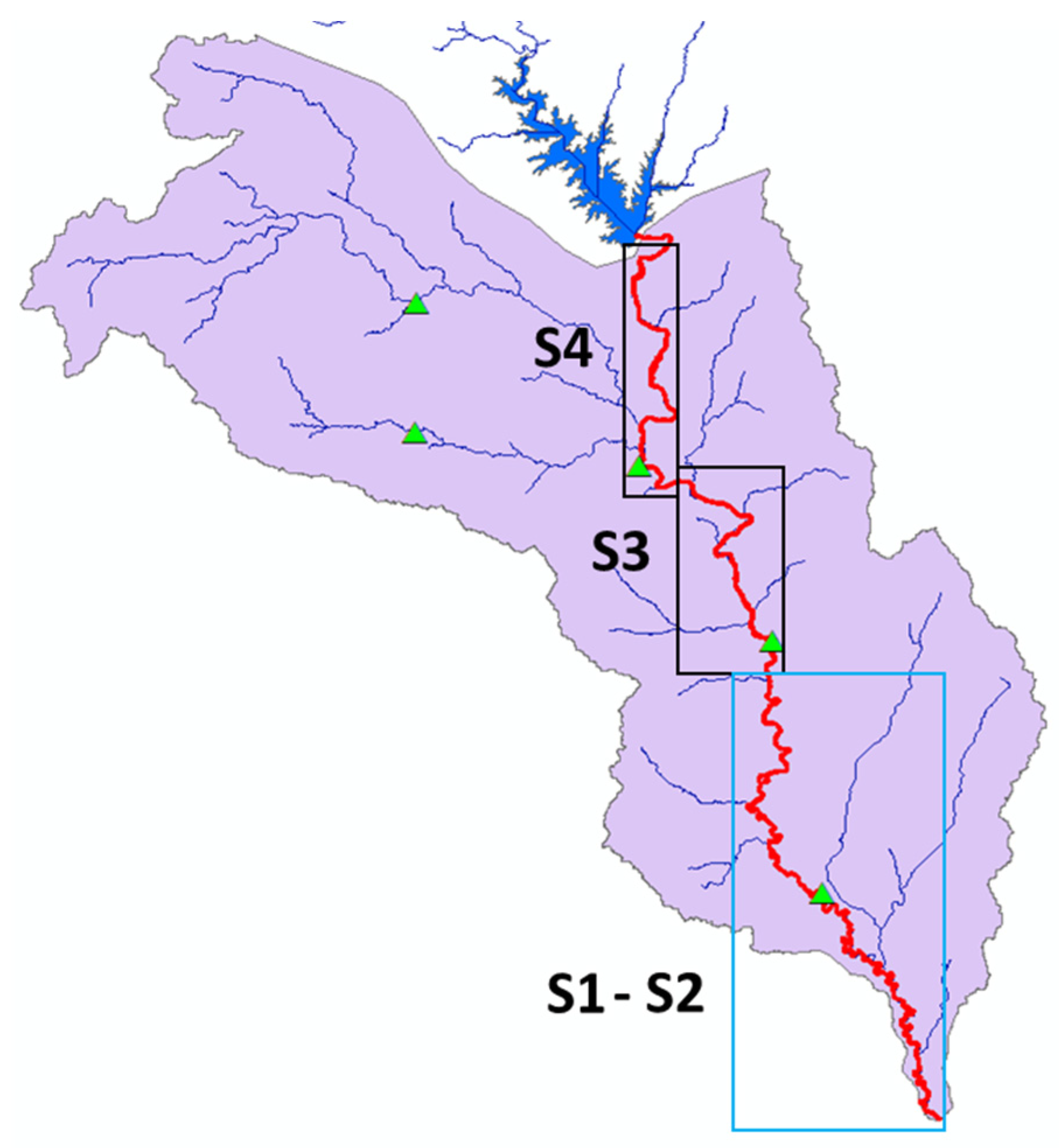
2.1. The Study Area

Located between latitudes 6.28° N and 9.39° N and longitudes 0.62° E and 1.99° E, the Mono river catchment extends over the territories of Benin (11%) and Togo (89%) Republics (Figure 1). It has a surface area of 23,736.64 km², and hosts the hydroelectric dam of Nangbéto.

The climate is sub-equatorial in the south and tropical in the northern part of the catchment. Main economic activities in the study area are small-scale farming, livestock breeding, fishing and trading. The average annual temperature recorded over the past 30 years ranges between 26 °C and 28 °C, with an average annual precipitation of 1200 mm. Land-use and land-cover types in the catchment are predominantly savannah, forest, croplands, settlements and water bodies. In this study, the entire Mono river catchment was used for hydrological modelling whereas only the portion of the river located downstream of the Nangbéto dam, and designated as the Lower Mono River (LMR), was considered for flood-hazard mapping with a hydrodynamic model. The downstream area of the catchment is characterized by low elevation and flat lands, which favor the persistence of flood events in the area. The main economic activities in the Mono catchment are agriculture, fisheries, livestock breeding and trade.

2.2. Data

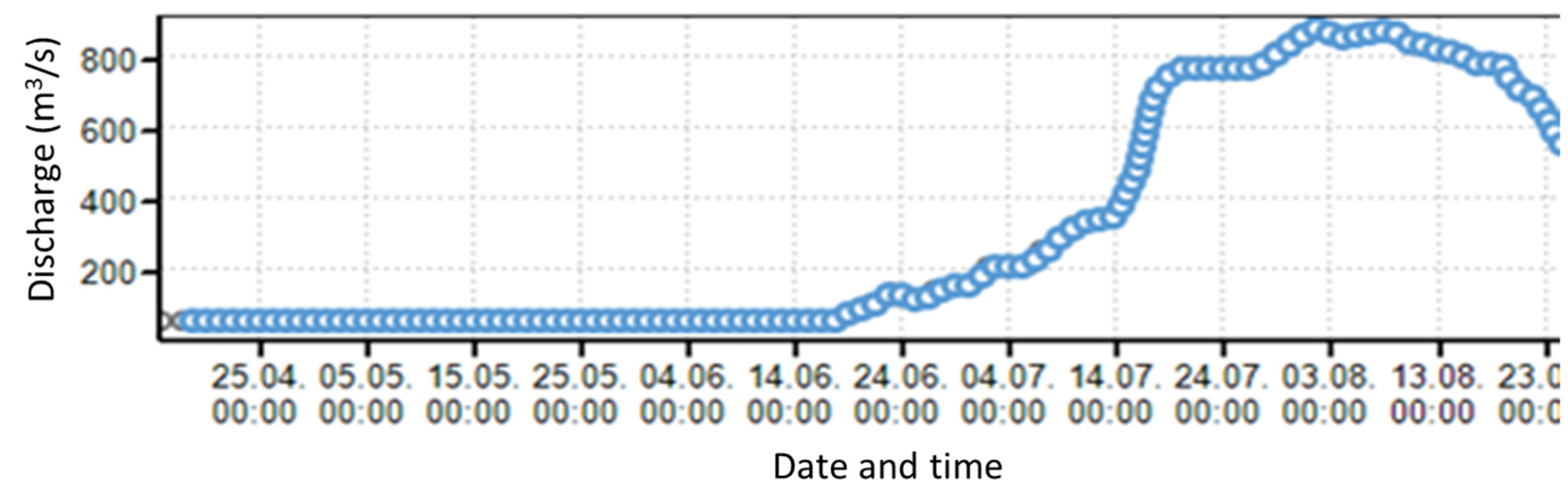
2.2.1. Hydro-Climatic Data

Precipitation and minimum and maximum temperature were collected for the period 1967–2010. Precipitation data was taken at 38 gauging stations and temperature from 3 synoptic stations. These observation data were provided by the meteorological services of Benin and Togo (METEO-Benin, DGMN-Togo). In addition, future precipitation and temperature data taken from the Coordinated Regional Downscaling Experiment (CORDEX) database, https://esgf-data.dkrz.de/projects/esgf-dkrz/ (accessed on 5 March 2020), were used. The period 2021–2070 was considered, and the Representative Concentration Pathways (RCP) scenarios RCP 4.5 and RCP 8.5 were used for future projections. Processed and ready-to-use climate-model data for future projection were provided by Houngue et al., 2022 [19] who systematically selected 6 Regional Climate Models (RCM) that were found to be the best performing in the Mono river basin. The 6 RCMs are shown in

Table 1. List of regional climate models used.

RCM	Institute	Driving Model	Designation
CCLM4-8-17	Climate Limited-area Modelling Community (CLMcom)	MOHC-HadGEM2-ES	MOHC-CCLM4
CCLM4-8-17	Climate Limited-area Modelling Community (CLMcom)	MPI-M-MPI-ESM-LR	MPI-CCLM4
RACMO22T	Royal Netherlands Meteorological Institute (KNMI)	ICHEC-EC-EARTH	ICHEC-RACMO22T
RCA4	Swedish Meteorological and Hydrological Institute (SMHI)	MOHC-HadGEM2-ES	MOHC-RCA4
RCA4	Swedish Meteorological and Hydrological Institute (SMHI)	MPI-M-MPI-ESM-LR	MPI-RCA4
REMO2009	Helmholtz-Zentrum Geesthacht, Climate Service Center, Max Planck Institute for Meteorology (MPI-CSC)	MOHC-HadGEM2-ES	MPI-REMO

.

Potential evapotranspiration (PET) was computed using the Hargreaves method [28]. The Hargreaves method (Equation (1)) is temperature-based and recommended when climate data such as wind speed, humidity, and solar radiation are lacking.

$${\mathrm{E}}_0=0.0023\times {\mathrm{H}}_0\times {\left({\mathrm{T}}_{\max }-{\mathrm{T}}_{\min }\right)}^{0.5}\times \left({\mathrm{T}}_{\mathrm{mean}}+17.8\right)$$

(1)

where ${\mathrm{E}}_0$ is PET (mm/day), ${\mathrm{H}}_0$ is extra-terrestrial radiation (MJ/m²/day), ${\mathrm{T}}_{\max }$ is the maximum air temperature for a given day (°C), ${\mathrm{T}}_{\min }$ is the minimum air temperature of the day (°C), and ${\mathrm{T}}_{\mathrm{mean}}$ is the mean air temperature of the day (°C).

This PET computation method was used due to data limitation in the study area, as reported in previous works [23,24,29]. In addition, it was reported that the well-known FAO (Penman–Monteith) method showed PET underestimation in the Mono basin, as opposite to temperature-based approaches [30]. As highlighted by Poméon et al. [31], who modelled streamflow in a dozen West African basins, including the Mono basin, the Hargreaves method is recommended when the quality of input data is questionable. In such circumstances, the Hargreaves approach is an effective alternative, with good results [32]. However, regardless of the computation method, daily PET estimates may be subject to error, due to daily fluctuations of climate variables [33].

Runoff data and rating curves were provided by the water directorate of Benin, DGEau-Benin, and the management of the Nangbéto dam (Centrale Electrique du Bénin, CEB) at 3 stations: Athiémé (1964–2010), Nangbéto (1987–2019) and Tététou (1965–1991). Runoff data were used for model calibration and validation.

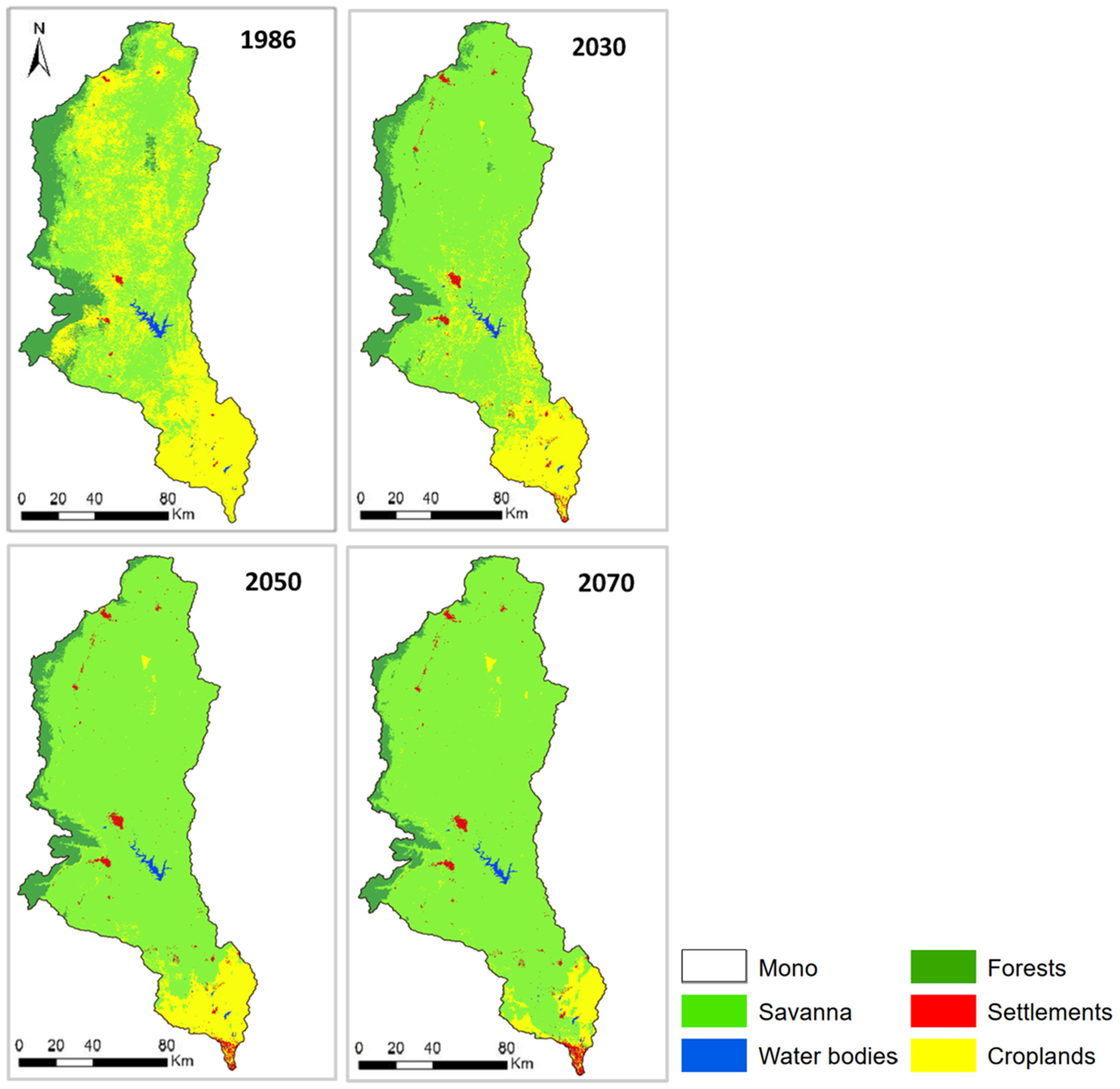
2.2.2. Land-Use and Land-Cover (LULC) Maps

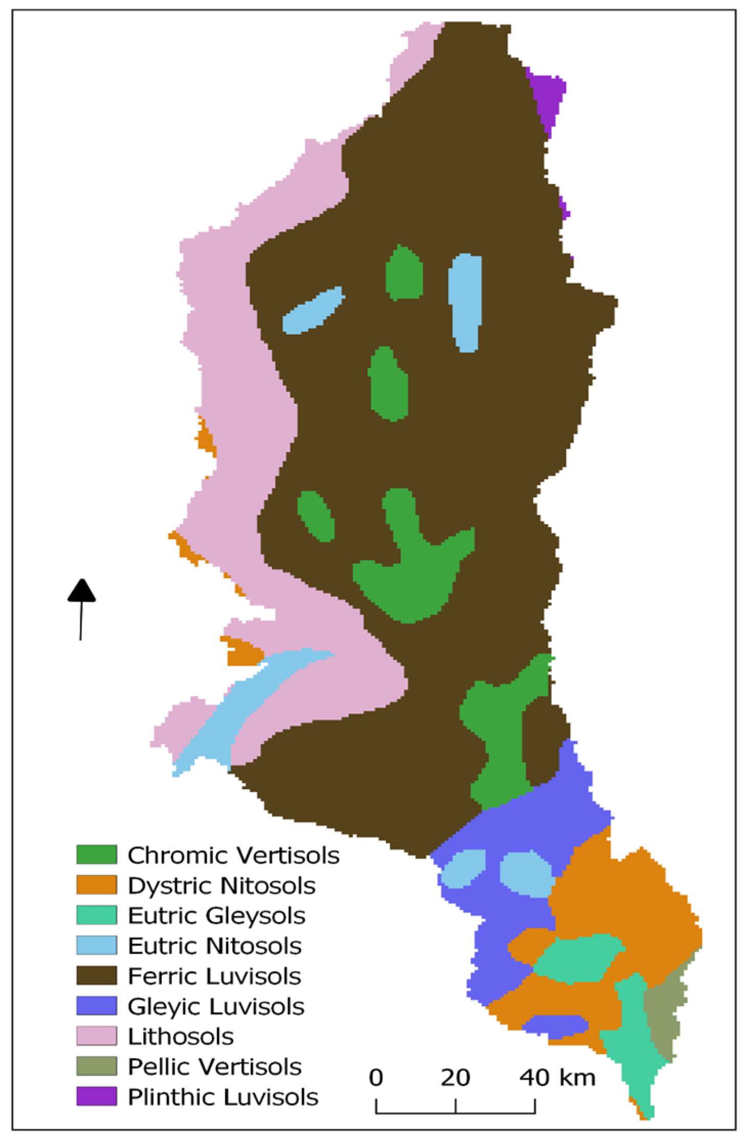
LULC maps from the past, 1986, and the future, 2030, 2050 and 2070 were used (Figure 2) as input in the runoff simulation. The maps were taken from the study of Thiam et al., 2022 [26]. They were classified and simulated using machine learning, stakeholders’ perspectives on land-use scenarios, and CA–Markov chain model embedded in the Land Change Modeler (LCM) of IDRISI software [26]. The LULC maps present 5 classes: savanna, forest, water bodies, settlement and cropland. The authors used the map from 2020 as a reference, to check the accuracy of the projections.

A classified LULC map from 2020 was compared to the one generated by the Land Change Modeler (simulated LULC map 2020) for the model validation. Good results were observed: the kappa index agreement resulted in a kappa for no information (Kno) of 0.91, a standard kappa (Kstandard) of 0.89, and a kappa for grid-cell-level location of 0.95 (Klocation). The LULC maps from 1986 to 2070 indicate a reduction in croplands and forests, while savanna and settlements are expected to continue to increase in the Mono river basin. Forest areas showed a 58% decrease, while settlements and built-up areas are expected to undergo a 384.47% increase. Land-use and land-cover changes in the Mono catchment are mainly driven by rapid population growth, overexploitation of lands, cities’ expansion and rainfall variability [25,26].

2.2.3. Soil Data

The soil map (Figure 3) was derived from the Harmonized World Soil Database (HWSD) v1.2 of the Food and Agriculture Organisation of the United Nations (FAO) https://www.fao.org/soils-portal/data-hub/soil-maps-and-databases/harmonized-world-soil-database-v12/en/ (accessed on 14 February 2020) and provides, among others, information on soil textures. Soil textures in the catchment are comprised of clay, loam and sandy-clay-loam. The map has a 30-arc-second resolution, about 1 km, and serves as the basis in the SWAT model for computation of the soil parameters (soil bulk density, water-storage capacity, and hydraulic conductivity), using pedotransfer functions.

The catchment is dominated by Luvisols, occupying 61.58% of the surface area. Luvisols are characterized by a higher proportion of clay in the subsoil than on the surface [34]. They have a sandy-clay-loam texture. The western part of the catchment, hosting the high elevation areas, is made of Lithosols, which cover 17.06% of the catchment area. Lithosols are usually found in mountainous regions and are characterized by rocks and gravelly or stony soils [34,35]. The rest of the catchment is made of Nitosols, Vertisols, and Eutric Gleysols, covering 11.26%, 7.44% and 2.47%, respectively, of the catchment area. The Vertisols have a clay texture, while Nitosols and the Eutric Gleysols are mainly made of loam.

2.2.4. Digital Elevation Model (DEM)

The digital surface model from the Advanced Land Observing Satellite (ALOS) provided by the Japan Aerospace Exploration Agency (JAXA) was used for elevation information. ALOS data has a 1 × 1 arc-second (about 30 m) resolution, and displays heights above sea level. As shown in Figure 1, elevation in the Mono catchment ranges from 0 to 922 m, with highest elevations located in the western and northern parts, while the downstream area in the south hosts the lowest elevations (Figure 1).

2.2.5. Reservoir Data

Two reservoirs were taken into account in this study: the reservoir of the existing Nangbéto dam, and that of the upcoming Adjarala dam. The Adjarala dam is located 100 km downstream of the Nangbéto dam. The characteristics of these reservoirs are shown in

Table 2. Reservoir characteristics.

Dam Parameter	Description	Unit	Value at Nangbéto	Value at Adjarala
MORES	Month the reservoir became operational		September	January
IYRES	Year the reservoir became operational		1987	2022
RES_ESA	Reservoir surface area when the reservoir is filled to the emergency spillway	ha	18,000	9500
RES_EVOL	Volume of the water needed to fill the reservoir to the emergency spillway	${10}^6{ \mathrm{m}}^3$	1715	630
RES_PSA	Reservoir surface area when the reservoir is filled to the principal spillway	ha	4200	8260
RES_PVOL	Volume of the water needed to fill the reservoir to the principal spillway	${10}^6{ \mathrm{m}}^3$	373.5	523
RES_VOL	Initial reservoir volume	${10}^6{ \mathrm{m}}^3$	373.5	523

CNEE, 2014 [27]; Houessou, 2016 [36].

.

The reservoir of the Nangbéto dam was represented as an existing reservoir, while the reservoir of Adjarala was simulated as a “scenario”, since the dam is not yet operational.

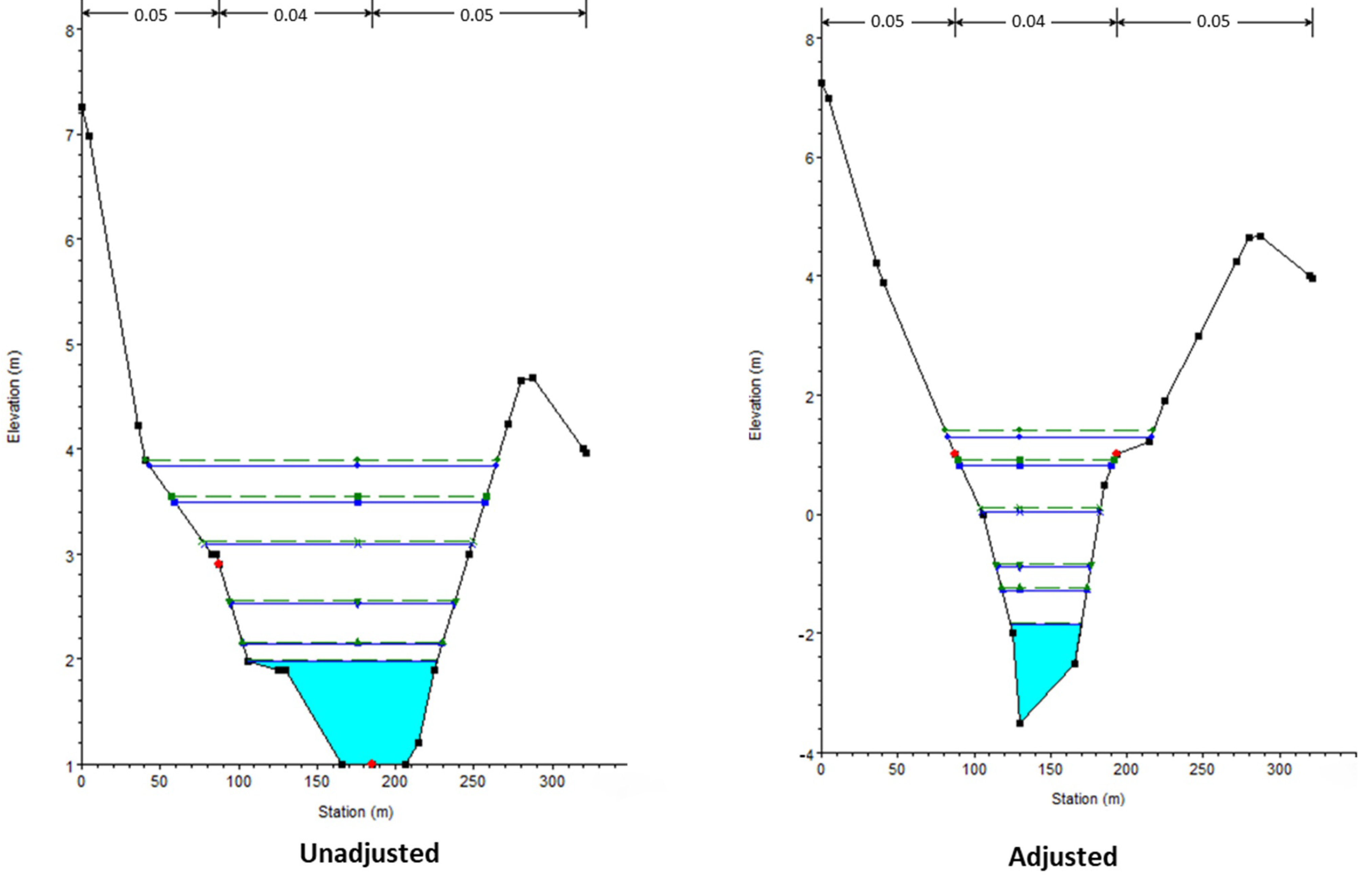
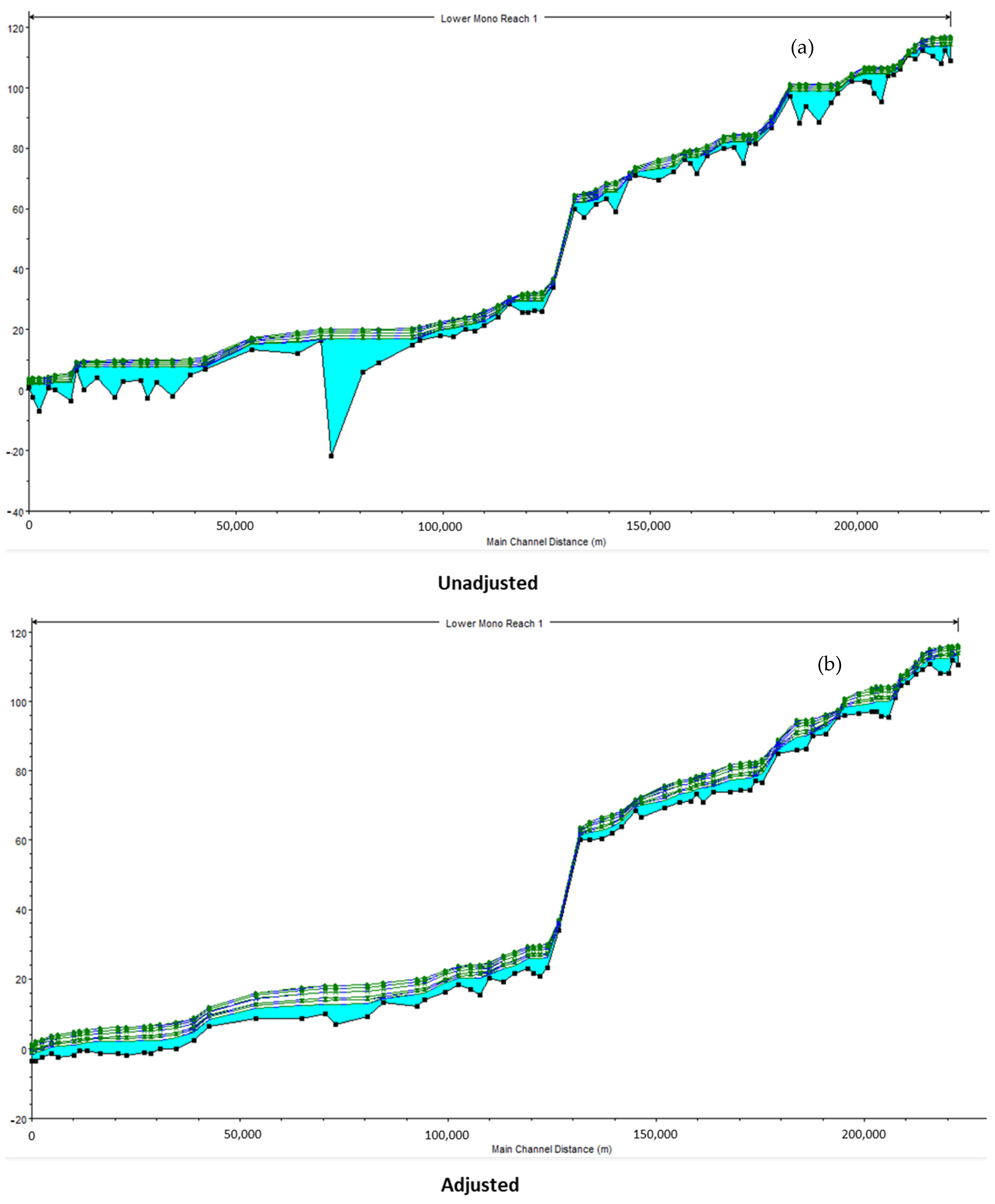
2.2.6. Cross-Sections

A good representation of river bathymetry is needed to adequately model the water flow in a river section. Cross-sections can be derived from field measurements and if field measurements are not available or possible, due to resource constraints, cross-sections can be extracted from DEM. However, caution should be observed when using DEM for the cross-section because of the resolution and errors on bed elevation, due to uncorrected water surface elevation. Due to COVID-19 travel restrictions, the fieldwork for cross-sectional measurement did not proceed according to what was initially planned. Because of this, cross-sections were derived by extracting the river-bed elevation from the DEM, and were corrected using the slope-area method supported by a 1D river model. ArcGIS, with the HEC-GeoRAS and HEC-RAS 1D model, was used as a tool to derive cross-sections, since these data were not available. The method behind this is elaborated on in Section 2.6 (a). Seventy-seven (77) cross-sections were derived, with their locations identified following the criteria of changes in width and slope and areas with meanders or bends.

2.3. River Runoff Simulation

The Soil and Water Assessment Tool (SWAT) is a physically-based hydrological model for water-quality and -quantity simulation. The water balance in SWAT is based on Equation (2) (Arnold et al., 2012) [37].

$${\mathrm{SW}}_{\mathrm{t}}={\mathrm{SW}}_{\mathrm{o}}+{\sum }_{\mathrm{i}=1}^{\mathrm{t}}\left({\mathrm{R}}_{\mathrm{d}}-{\mathrm{Q}}_{\mathrm{surf}}-{\mathrm{ET}}_{\mathrm{a}}-{\mathrm{W}}_{\mathrm{perc}}-{\mathrm{Q}}_{\mathrm{gw}}\right)$$

(2)

where ${\mathrm{SW}}_{\mathrm{t}}$ is the final soil-water content; ${\mathrm{SW}}_{\mathrm{o}}$ the initial soil-water content; ${\mathrm{R}}_{\mathrm{d}}$ the amount of precipitation, ${\mathrm{S}}_{\mathrm{surf}}$ the surface runoff, ${\mathrm{ET}}_{\mathrm{a}}$ the evapotranspiration, ${\mathrm{W}}_{\mathrm{perc}}$ the percolation, and ${\mathrm{Q}}_{\mathrm{gw}}$ the amount of return flow on day i.

SWAT has been used successfully, with good results, in various West African catchments [38] such as the Niger basin [39,40], the Volta basin [41,42] and the Ouémé basin in Benin [43,44]. Koubodana et al., 2021 [23] applied SWAT to the Mono river catchment and also reported good results.

As a semi-distributed model, SWAT splits the catchment into sub-basins that are further divided into hydrological response units (HRU). An HRU is a unique combination of land use, soil type and slope. HRU are the computation units in SWAT [45]. For the Mono river catchment, 153 sub-basins and 552 HRUs were derived.

The impacts of climate and LULC changes on the runoff of the Mono river were evaluated over the period 2022–2070. In order to account for the continuous LULC change in the catchment, the LULC map from 2030 was used for the period 2022–2030, the map from 2050 for the period 2031–2050, and the map from 2070 for 2051–2070.

This study used the sequential uncertainty fitting, SUFI-2, embedded in the calibration and uncertainty programs, SWAT-CUP v5.1.6, for calibration, sensitivity analysis and uncertainty analysis. One specificity of SWAT-CUP is that its calibration parameters are not assigned single values; rather, intervals are defined. This approach accounts for the uncertainties in the definition of parameter value, because nothing like a unique perfect set of parameters exists [46]. For that purpose, a 95% prediction uncertainty (95PPU) is calculated at the 2.5% and 97.5% levels of the cumulative distribution of the output variable obtained through Latin hypercube sampling.

The calibration and validation periods were identified based on the available data, the peak flow events, and the construction of the Nangbéto dam. Discharge data for the Mono river catchment are characterized by a substantial level of missing values, especially after the construction of the Nangbéto dam in 1987. From 1967–2010, 28% of discharge records are missing, out of which 72% are in the period 1988–2010, and occurred mainly during the high-flow period of April–October. Since the focus of this study is on flood events, only years with no more than 30% missing data between April and October were used. These are 1964–1986, 1988, 1989, 1990, 1991, 1992 and 2010. The first 3 years, 1964–1966, were used as a warm-up period. As recommended, the different hydrological events in the study area should be accounted for during both the calibration and the validation phases, and the mean and standard deviation should be similar during the two periods [47]. In that regard, the calibration period was made up of the years 1967–1977, 1990, 1991, and 1992, and the model was validated for 1978–1986, 1988, 1989 and 2010. The two periods contain years before and after the construction of the dam, as well as low and high peaks. The mean discharge values during calibration and validation are 106.40 m³/s and 111.38 m³/s respectively, while the standard variations are 177.15 m³/s and 170.40 m³/s.

Thirteen (13) calibration parameters were selected, based on previous studies in Benin and Togo [29,40,48], and in the West African region [31,49,50]. The Global Sensitivity program embedded in SWAT was used to assess the sensitivity of the parameters after a 1000-run simulation.

Table 3. SWAT calibration parameters.

Rank	Parameter	Definition	Range
1	r_CN2	SCS runoff curve number	−0.5–0
2	r_ESCO	Soil-evaporation compensation factor	−0.4–(−0.1)
3	v_GW_REVAP	Groundwater “revap” coefficient	0.04–0.12
4	r_SOL_AWC	Available water capacity of the soil layer	0–0.5
5	r_SOL_BD	Moist bulk density	−0.1–0.5
6	v_RCHRG_DP	Deep-aquifer percolation fraction	0–0.5
7	v_REVAPMN	Threshold depth of water in the shallow aquifer for “revap” to occur	70–120
8	r_SOL_K	Saturated hydraulic conductivity	−0.3–0.3
9	v_GWQMN	Threshold depth of water in the shallow aquifer required for return flow to occur	600–1200
10	v_GW_DELAY	Groundwater delay	5–15
11	v_ALPHA_BF	Baseflow alpha factor	0.1–0.3
12	v_SURLAG	Surface-runoff lag time	5–15
13	r_EPCO	Plant-uptake compensation factor	−0.3–0.3

presents the list of parameters, their ranking based on the sensitivity analysis, and the ranges used. The goodness-of-fit between simulation and observation was based on the Kling-Gupta efficiency (KGE) [51], the coefficient of determination (${\mathrm{R}}^2)$ and the percentage of bias (PBIAS). In addition, the p-factor and r-factor provided by the SUFI-2 program, indicate respectively the percentage of measured data bracketed by the 95PPU, and the average thickness of the 95PPU band divided by the standard deviation of the measured data.

With the assumption of all being equal, these parameter values were applied to simulate future climate- and land-use-change impacts on the runoff of the Mono river.

2.4. Runoff and Flood Scenarios

Five scenarios organized in 3 groups are investigated in this study: a base-case scenario, scenarios without the Adjarala dam, and scenarios with the Adjarala dam. The base-case (BC) scenario has been the reference situation since the construction of the Nangbéto dam. It serves as a basis for comparison, and represents the past-to-present conditions in the catchment. The year of construction of the Nangbéto dam is taken as the starting point of the BC, in order to assure similar hydrological conditions when comparing past-to-present runoff with projected ones.

The scenarios without the Adjarala dam are scenarios that account simultaneously for climate- and land-use-change projections. Climate- and land-use-change scenarios were not simulated separately, but concomitantly and in subsets, in the SWAT model. The projected climatic data from 2022 to 2030 are used together with the LULC map from 2030 to simulate runoff from 2022 to 2030; likewise, for the period 2031–2050 (and 2051–2070), climate data from 2031 to 2050 (and 2051–2070) is used in combination with the LULC map from 2050 (and 2070) to obtain runoff projections for the period under consideration. Therefore, the scenarios referred to as RCP 4.5 and RCP 8.5 in this study already embed LULC scenarios, and stand for “RCP 4.5 + LULC scenario” and “RCP 8.5 + LULC scenarios”, respectively.

Scenarios with Adjarala consist of climate scenarios and LULC scenarios simulated together with the Adjarala dam. They are referred to as “RCP 4.5 + Adjarala dam” and “RCP 8.5 + Adjarala dam”, respectively.

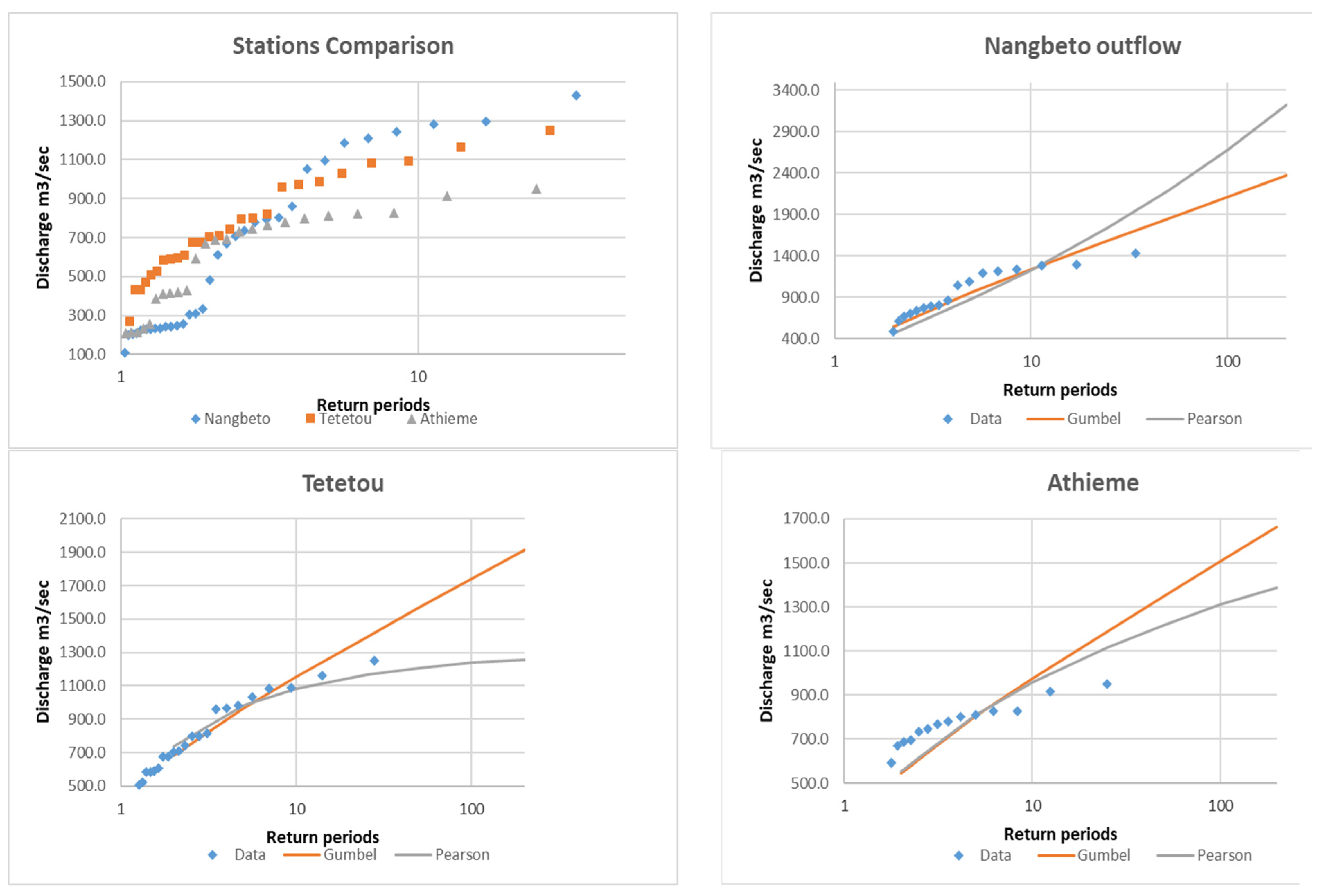
2.5. Flow Trend and Pattern Analysis

The trend of discharge was assessed using the Mann–Kendall test [52] at 95% confidence level. The Z statistics from the Mann–Kendall test indicate the trend (increasing or decreasing) and the significance of the test. A positive Z means an increasing trend, while a negative value suggests a decrease in the time series. The result of the test is considered to be statistically significant (and not significant) when Z > 1.96 (Z < 1.96). The Man–-Kendall test was applied to the time series of daily discharge under the scenario RCP 4.5 and RCP 8.5.

Mean hydrographs were derived to analyze the overall pattern of the flow in a year. The mean hydrographs were obtained by averaging the daily discharge over all the years of the study period. The mean hydrographs were derived for the scenarios RCP 4.5 and RCP 8.5, before and after the construction of the Adjarala dam.

In addition to the mean hydrographs, flow-duration curves (FDCs) were used to assess the effects of the yet-to-be-built Adjarala dam. FDCs are obtained with the following steps:

• Discharge records are ordered from the highest to lowest values, and each discharge value is assigned a rank $r$, $r=1,\dots ,n$, where n is the total number of records and 1 is assigned to the largest value;
• Probabilities of exceedance are calculated as:

  $$p=\frac{r}{n}\times 100$$

  (3)
• Discharge values are represented on the y-axis, with a logarithmic scale, and the probabilities of exceedance on the x-axis, with an arithmetic scale.

The probability of exceedance indicates the percentage of time that a given discharge is equaled or exceeded [53], e.g., when a discharge value Q has a percentage of exceedance p, it does not mean that the discharge is Q for p% of the time, but that Q is equaled or exceeded p% of the time. The shape of the FDC informs on the hydrological characteristics of the stream under consideration. A very curved FDC shows the flashy or ephemeral state of the stream; a steep shape in the upper end indicates that high runoffs in the study area are caused by rainfall, unlike snowmelt floods, which would depict a flatter shape at the upper end of the curve [54]. A flat slope at the lower end of the FDC indicates a high storage or a regulation of the streamflow (either artificially or naturally), while a steep slope indicates a lower storage [55]. In this study, discharges with 0–5% percentage of exceedance are characterized as extremely high, 5–20% as high, 20–70% as medium, 70–95% as low, and 95–100% as extremely low [56].

2.6. Flood-Hazard Simulation

Flood (hazard) or a hydrodynamic model can be a valuable tool to support flood-emergency managers and planners in making decisions, as well as creating community awareness to mitigate the impact of flooding. Flood models can be used for both event and long-term management of floods, and this can be from near-real-time flood forecasting to understanding the impact of future scenarios in the context of climate and land-use change and evaluating the adequacy of current and planned mitigation measures. Such examples are the work of Icyimpaye et al. (2022) [57] in the Nyabugogo River in Rwanda, and Komi et al. (2017) [58] in the Oti River basin in West Africa. These studies coupled together the hydrological and hydrodynamic models to forecast flooding and to assess the effectiveness of the proposed measures to mitigate the impact of floods.

Flood models can be classified into one dimension (1D), or 2D, or a coupled 1D–2D model. Due to the nature of the directional flow of water in rivers and floodplains, 1D models are generally used for simulating water flow in the channel and 2D for the floodplain. However, for wide rivers, a 2D model can also be used to simulate water flow, because water may also flow in 2 dimensions. 2D models often require more computational time and resources compared to 1D; nevertheless, this type of model is really useful for spatio-temporal hazard-impact assessment, because it provides you with a better understanding of, and information about, the affected area. Mitsopoulos et al. (2022) [59] presented an interesting study on the coupling and optimizing of a 1D and 2D hydrodynamic model, using HEC-RAS for early warning of flash floods. Compared to just a 1D or 2D hydrodynamic mode, the coupling of 1D and 2D yielded a faster simulation, with spatial information on flooding in the floodplain.

In the current case study, the TELEMAC-2D developed by Laboratoire National d’Hydraulique et Environnement (LNHE), part of the R&D group of Électricité de France, was used. It simulates free-surface flows in two dimensions of horizontal space, solving the Saint-Venant equations using the finite-element or finite-volume method in a computational mesh of triangular elements. For pre- and post-processing of the TELEMAC-2D model, the Kalypso 1D/2D software from Björnsen Consulting Engineers (BCE) GmbH Germany was used. It presents a structured user-oriented graphical unit interface to visually set up the model (https://kalypso.bjoernsen.de (accessed on 5 March 2020)). ArcGIS with the HEC-GeoRAS and HEC-RAS 1D model was used as a tool to derive cross-sections, since these data were not available.

(a)

Data input pre-processing

A representative cross-section is required for the hydrodynamic model to simulate adequately the flows in the channel. A measured cross-section is the most ideal representation, although alternatively, a DEM-derived cross-section can be an option. However, DEM river-bed elevations are often time erroneous, and thus correction is needed. In this research study, due to the lack of measured cross-sections, seventy-seven cross-sections were derived using the 30 m DEM, and this was corrected using the slope-area method (Equation (4)). The DEM cross-section was extracted using the HEC-GeoRAS tool, and adjustments were supported and verified using the HEC-RAS 1D modelling tool. The following are examples of adjusted and unadjusted cross-sections (Figure 4 and Figure 5).

$$Q=\frac{1}{n}A{R}^{\frac{2}{3}}{S}^{\frac{1}{2}} \to \frac{Q\times n}{S^{\raisebox{1ex}{$1$}\!\left/ \!\raisebox{-1ex}{$2$}\right.}}=\frac{{\left(\raisebox{1ex}{$x$}\!\left/ \!\raisebox{-1ex}{$4$}\right.\right)}^{\raisebox{1ex}{$5$}\!\left/ \!\raisebox{-1ex}{$3$}\right.}\times {\left(y\right)}^{\raisebox{1ex}{$5$}\!\left/ \!\raisebox{-1ex}{$3$}\right.}}{{\left({\left(x^2+4y^2\right)}^{\raisebox{1ex}{$1$}\!\left/ \!\raisebox{-1ex}{$2$}\right.}\right)}^{\raisebox{1ex}{$2$}\!\left/ \!\raisebox{-1ex}{$3$}\right.}}$$

(4)

where

• $Q=$ discharge (m³/s)
• $n=$ Manning’s roughness coefficient (range between 0.01 and 0.75)
• $A=$ cross-section area (m²)
• $R=$ the hydraulic radius, equal to the area divided by the wetted perimeter (m)
• $S=$ the head-loss per unit length of the channel, approximated by the channel slope

Figure 4. Example section of unadjusted and adjusted cross-section. Bank location is presented by the red mark; the left-hand figure shows that the location of the right bank is in the river bed. The right-hand figure presents the corrected bank elevation and channel depth.

Figure 4. Example section of unadjusted and adjusted cross-section. Bank location is presented by the red mark; the left-hand figure shows that the location of the right bank is in the river bed. The right-hand figure presents the corrected bank elevation and channel depth.

Figure 5. Longitudinal profile of the unadjusted (b) and adjusted (a) cross-section, presenting the lowest bed elevation of the 77 cross-section. Ideally, rivers follow a constant slope. Due to DEM errors, the left-hand figure shows an irregular slope between the cross-section. After correcting all cross-sections, the longitudinal profile shown in (b) now has a constant slope.

Figure 5. Longitudinal profile of the unadjusted (b) and adjusted (a) cross-section, presenting the lowest bed elevation of the 77 cross-section. Ideally, rivers follow a constant slope. Due to DEM errors, the left-hand figure shows an irregular slope between the cross-section. After correcting all cross-sections, the longitudinal profile shown in (b) now has a constant slope.

Different land uses can affect water flow, where the greater the roughness coefficient the lesser the flow velocities. To represent this in the equations, an empirically derived roughness coefficient is introduced, using the table from Chow (1959) [60] approximating it to Ks values. Landsat satellite imagery (present time) was used for the identification of land-use types, based on the works of Thiam et al. (2022) [26].

As a requirement for the model, using ArcGIS, the river and its banks and DEM spatial-model boundary and distinct features (e.g., roads) were delineated and exported to shape and ascii files, respectively.

(b)

Model setup

The LMR was initially divided into four sections (S1–S4) for the reasons of model run-time efficiency, availability of historical discharge and flexibility in the integration of scenarios and measures. However, during the first investigation and run analysis, it was decided to combine the S1 and S2 (Figure 6) sections because of the rather flat terrain in these sections. Coupling these two sections allowed us to have a better representation of the flow and interaction of floodwater in the terrain. Furthermore, knowing that computational parallelization is possible, a multi-core CPU were used when running the model. Measured discharge was used for calibration and for climate- and land-use-change scenarios, and for the planned Adjarala dam the hydrologically derived discharge model was used.

Table 4. Model set-up of the three sections.

Input Data	Section
	S1–S2	S3	S4
DEM	30 m	30 m	30 m
River bathymetry	30 m DEM—Corrected theoretically Length—139.5 km	30 m DEM—Corrected theoretically Length—52.83 km	30 m DEM—Corrected theoretically Length—53.11 km
Land use for flow resistance	Farmland, water, settlement and savanna	Farmland, water, settlement and savanna	Farmland, water, settlement and savanna
Mesh 2D elements	Number of elements—477,889 Area—2064 km2	Number of elements—174,876 Area—182.7 km2	Number of elements—183,325 Area—237 km2
Upstream boundary	Athiémé/Adjarala discharge	Tététou discharge	Nangbéto discharge
Downstream boundary	Sea-water level (constant)	Athiémé/Adjarala rating curve	Tététou rating curve
Discharge time series	August 2010–April 2011	August 2010–April 2011	August 2010–April 2011
Rating curve	Not available	Yes	Yes

presents the summary of the set-up of the sections.

In setting up the model in Kalypso, the discharge data was imported, the location of the model boundary was defined, a computational mesh to represent the river and floodplain was created, the mesh elevation and roughness coefficient were assigned, upstream and downstream boundary conditions were defined, and calculation units and simulation settings were set. At the end, the model set-up was exported to a file format for Telemac2D, and the model was run using the command line terminal script for Telemac2D.

(c)

Calibration and validation

Calibration of a hydrodynamic model generally makes use of the observed-water-level data, to compare it with the model output. However, due to the unavailability of observed-water-level data, the model results were calibrated and validated by comparing them with a satellite image of a flooding event with a similar discharge. Moreover, stakeholders were also engaged in a workshop on identifying the most flood-prone areas, based on their field and expert knowledge.

In this context, first, the low- and medium-flow discharge was used to simulate a full riverbank. Then the 1963 and 2010 extreme events were used as reference cases, for comparison with satellite imagery of a similar flood discharge in the year 2019. The 1963 and 2010 extreme events had a maximum peak discharge at Athiémé of about 900 m³/s. Flooding in the Mono river, as shown in Figure 7, can last up to several months. Thus, the model has to run a 70-to-90-day event to capture the rise and fall of the water level in the Mono river.

The extreme event was spatially validated with the processed satellite imagery from MODIS by UNOSAT for the flood event of 2019 (https://unosat.org/products/2763 (accessed on 5 March 2020)) and inputs from the stakeholder workshop (Figure 8). Unfortunately, UNOSAT published a flood map that only shows the side of Togo. Hence, the southeastern coastal part is not presented. The flood event of 2010 was more or less comparable to that of 2019 in terms of peak discharge. The results show an almost similar flood extent. However, remotely sensed information cannot capture shallow water depths, which is why some parts look as if there is no flooding.

2.7. Analysis of Extremes and Flood-Hazard Scenarios

For the analysis of extremes, max-discharge return periods (HQ) of 2, 5, 10, 50 and 100 years were statistically derived for the historical (base case) and future scenarios. The extreme value distribution (EVD) statistical analysis of Gumbel (GEV) and Pearson III were used to derive HQ for stations Nangbeto, Tetetou and Athieme. The work of Millington et al. (2011) [61] presented an interesting study on the comparison of GEV and Pearson III in the upstream of the Thames river basin under different global climate models. In the Lower Mono case study, GEV was used, because it represents the trend of the recorded HQs.

For the base case, discharge data of 33 years (1987–2019) were used for Nangbéto station, 27 years (1965–1991) for Tététou and 24 years (1987–2010) for Athiémé. Future scenarios on climate (RCP 4.5 and 8.5) and land-use change, with and without the Adjarala dam from the years 2022 to 2070 were used to derive future return periods (HQs) of discharge. Estimates of discharge with future scenarios were modelled using the hydrological model at the station at Athiémé. Figure 9 presents the plot of the base case HQ.

After the analysis of extremes, these HQs were transformed into a hydrograph (Figure 10), having the shape derived from several high-flow-event hydrographs. This was then used as an input for the hydrodynamic model, to obtain an idea of the severity of these flooding scenarios.

3. Results and Discussion

3.1. Runoff Simulation

3.1.1. Model Calibration and Validation

Figure 11 shows the simulation results during the calibration and validation phases. A visual inspection indicates that the pattern of observed discharge at the Athiémé station is well represented. This is supported by the statistics presented in

Table 5. Goodness-of-fit during SWAT calibration and validation.

Goodness-of-Fit	KGE	R2	PBIAS	p-Factor	r-Factor
Calibration	0.83	0.80	−13	0.91	1.31
Validation	0.68	0.57	2.3	0.85	1.46

.

Overall, the values of p-factor and r-factor show that the parameter ranges that were used represent well the observation, and with relatively low uncertainty. As reported by Schuol et al., 2008 [49], a p-factor and a r-factor near 1 indicate fairly good results. The p-factor of 0.91 during calibration (0.85 during validation), means that 91% (85%) of observation was bracketed within the 95% certainty range, defined by the 95PPU band. Moreover, the ability of the model to capture the flow during the period 1970–1985, which is known as a drought-dominated period over West Africa [62], and the capacity of the model to represent the peaks, confirms the good performance of the SWAT model in both drought and flood periods in the Mono basin. The lower R² and KGE statistics noticed during validation are imputable to the abnormally high values simulated at the beginning of 2010. This overestimation may be due to outliers in the rainfall records. Despite this lower R² value, the model showed good results during validation, compared to the calibration statistics, which were also very good. In addition, the bias level declined during the validation period. The fact that the calibration and validation periods were not selected as continuous periods (e.g., 1967–1976 and 1977–1986), but were rather based on a balanced combination of hydrologic conditions (dam and no-dam years, high- and low-peak years), has led to better results, compared to a previous study conducted with SWAT in the Mono catchment [29]. In the study by Koubodana et al., 2021 [29], known to date as the only published work with SWAT in the Mono catchment, the authors created two distinct models: one for the period before the Nangbéto dam construction (1964–1986), and another one for the period after the dam (1988–2011). The model calibration with that approach yielded very good results for the period before the construction of the dam (KGE = 0.82, R² = 0.68), but a lower performance during the post-dam period (KGE = 0.54, R² = 0.2). The decline in the statistics may be attributed to the high level of missing discharge data during the post-dam period of 39% (the majority occurring in the high-flow season), which substantially reduced the actual exploitable data.

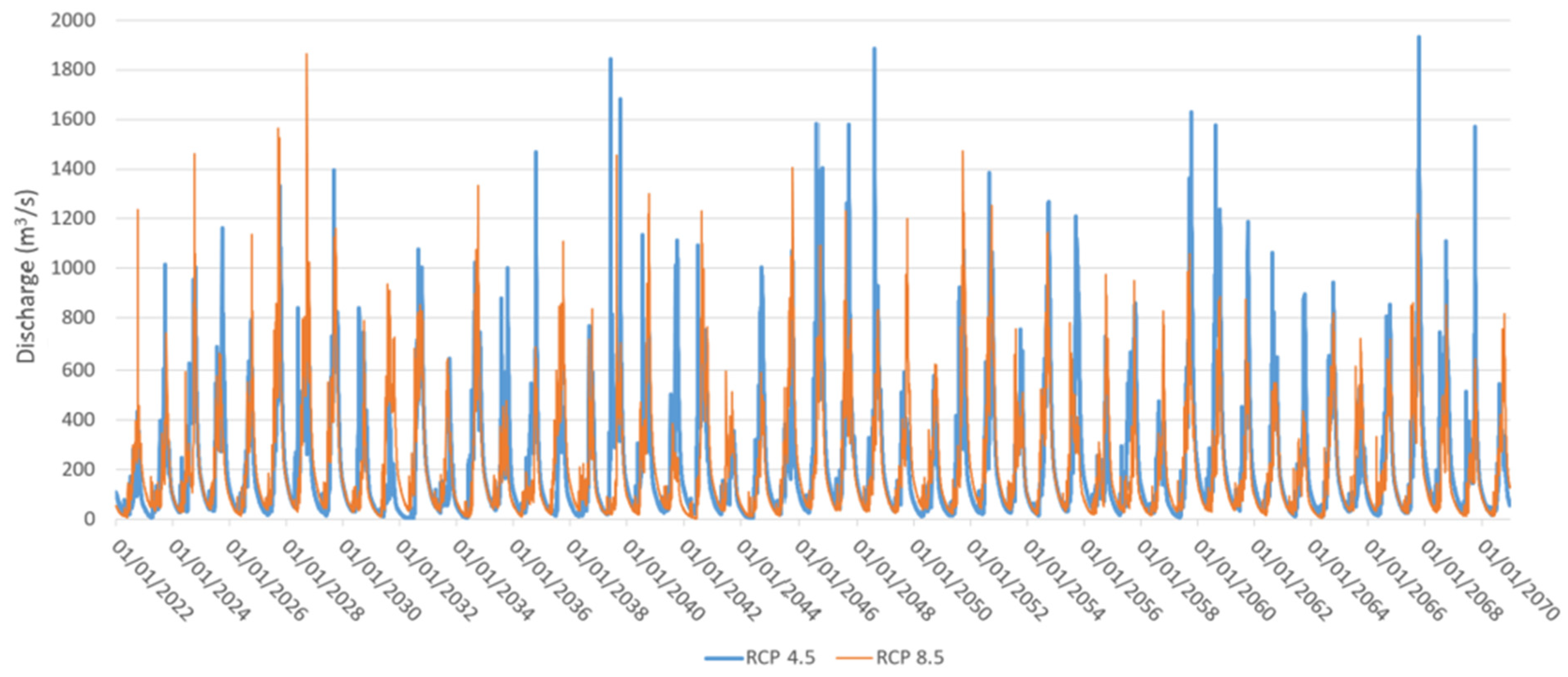
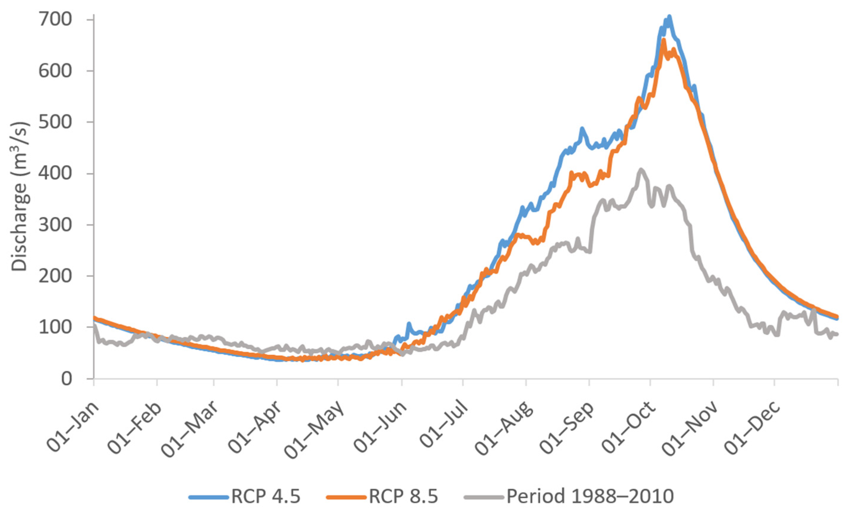
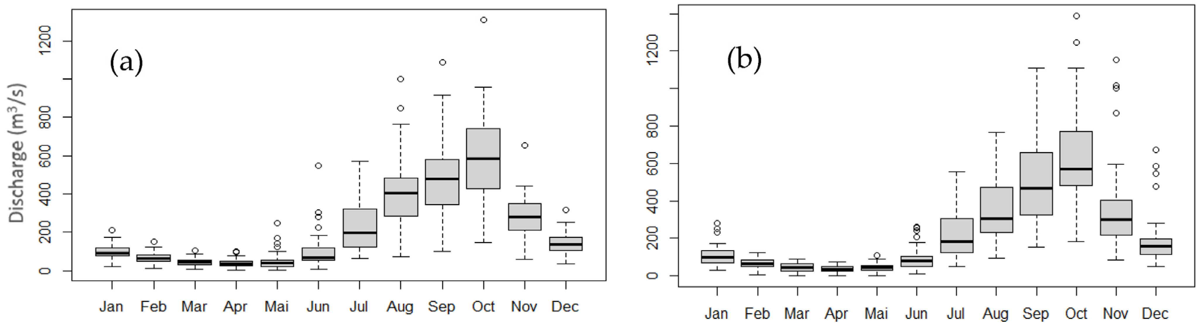
3.1.2. Future Runoff under Climate- and Land-Use-Change Scenarios

Figure 12 presents the pattern of the discharge under climate- and land-use-change scenarios.

During the period 2022–2070, the runoff is expected to be characterized by a mixture of high and low peaks. The scenario RCP 4.5 projects higher peak values than the scenario RCP 8.5. This is attributable to rainfall and temperature projections in the Mono River basin. As reported by Houngue et al., 2022 [19], RCP 4.5 projects wetter conditions (higher precipitations peaks and lower temperatures) than the high-pathway scenario, RCP 8.5, in the Mono basin. With reference to 1966–2015, the average annual temperature in 2021–2070 presented a 1.5 °C increase under RCP 8.5, while the intermediate-pathway scenario, RCP 4.5, showed a 1 °C increase.

The Mann–Kendall test performed on annual peaks of runoff from 2022 to 2070, revealed a statistically-insignificant increase with the scenario RCP 4.5 (p-value = 0.53), and a significant decrease under RCP 8.5 (p-value = 0.04). This is in line with the rainfall and temperature scenarios mentioned above. However, regardless of the projected trend, a succession of low and high annual peaks are expected in some years; for instance, 2058 (464.5 m³/s) and 2059 (1629 m³/s) under RCP 4.5, and the years 2045 (592.1 m³/s) and 2046 (1407 m³/s) under RCP 4.5.

The highest discharge recorded in the Mono catchment, from 1960 to 2010, is about 900 m³/s, and was observed in 1963 and in 2010. That discharge magnitude triggered one of the most disastrous flood events in the catchment [13,14]. Taking 900 m³/s as a reference during the period 2022–2070, it was noticed that the discharge under RCP 8.5 has more years (24 years) above 900 m³/s than the scenario RCP 4.5 (19 years). This means that, despite the lower peak values projected by the scenario RCP 8.5, potentially high flood events are likely to occur often under that scenario. That assumption is corroborated by the discharge values at return periods 2, 5, 10, 50, and 100.

Table 6. Return periods of runoff with climate- and land-use-change scenarios.

	Runoff (m3/s)
Return Period	Base Case	RCP 4.5	RCP 8.5
2	554.80	1014.32	927.28
5	810.30	1373.82	1228.53
10	956.2	1584.36	1408.91
50	1218.00	1981.44	1758.66
100	1308.50	2125.34	1889.02

presents the return period and associated discharge values for scenario RCP 4.5 and RCP 8.5, and for the base-case scenario.

Comparing the base case (BC) with the future scenarios shows that the peak runoff becomes more frequent in the future. For example, the base case HQ10 will become HQ2.

Figure 13 presents the mean hydrograph for the period 1988–2010 (after the construction of the Nangbéto dam) and the hydrographs under future climate- and land-use-change scenarios.

Overall, the peaks are expected to increase during 2022–2070, with a longer overland flow. This is attributable to rainfall projections in the Mono catchment, which are expected to be more intense due to climate and land-use changes. As reported by Amoussou et al., 2020 [20], the annual maximums of daily precipitation are expected to increase between 2028 and 2050. The authors assessed extreme rainfall patterns in the Mono catchment, and concluded that a significant increase in the intensity of extreme rainfall events is expected. The analysis of the precipitation data used in this study revealed an increase in peaks, a delay in the start of the rainy season, and a shorter season [19]. Moreover, the findings of the study of Wetzel et al., 2022 [63] on assessing flood-risk dynamics in the LMR shows that there is a strong causality between economic dependence on agriculture and the destruction of ecosystems and soil degradation, which are driven by the type of agriculture and the agricultural techniques. This soil degradation and destruction of ecosystems will also have an impact on the extremity of the flooding. This will produce more run-off and sedimentation in the river channels. Those factors, compounded with the decrease in forest areas and the extension of settlements in the catchment [25,26] may trigger low infiltration rates and a higher runoff. The works of Thiam et al., 2022 [26] shows a 58% decrease in forest in the year 2070, which would have an effect on the ecosystems and soil degradation.

The boxplots in Figure 14 illustrate the interannual variability of discharge under the scenarios RCP 4.5 (a) and RCP 8.5 (b).

Despite the projected overall increase in discharge, high interannual variabilities are expected at a monthly scale, especially during the high peak season. The highest variations are noticed from July to November.

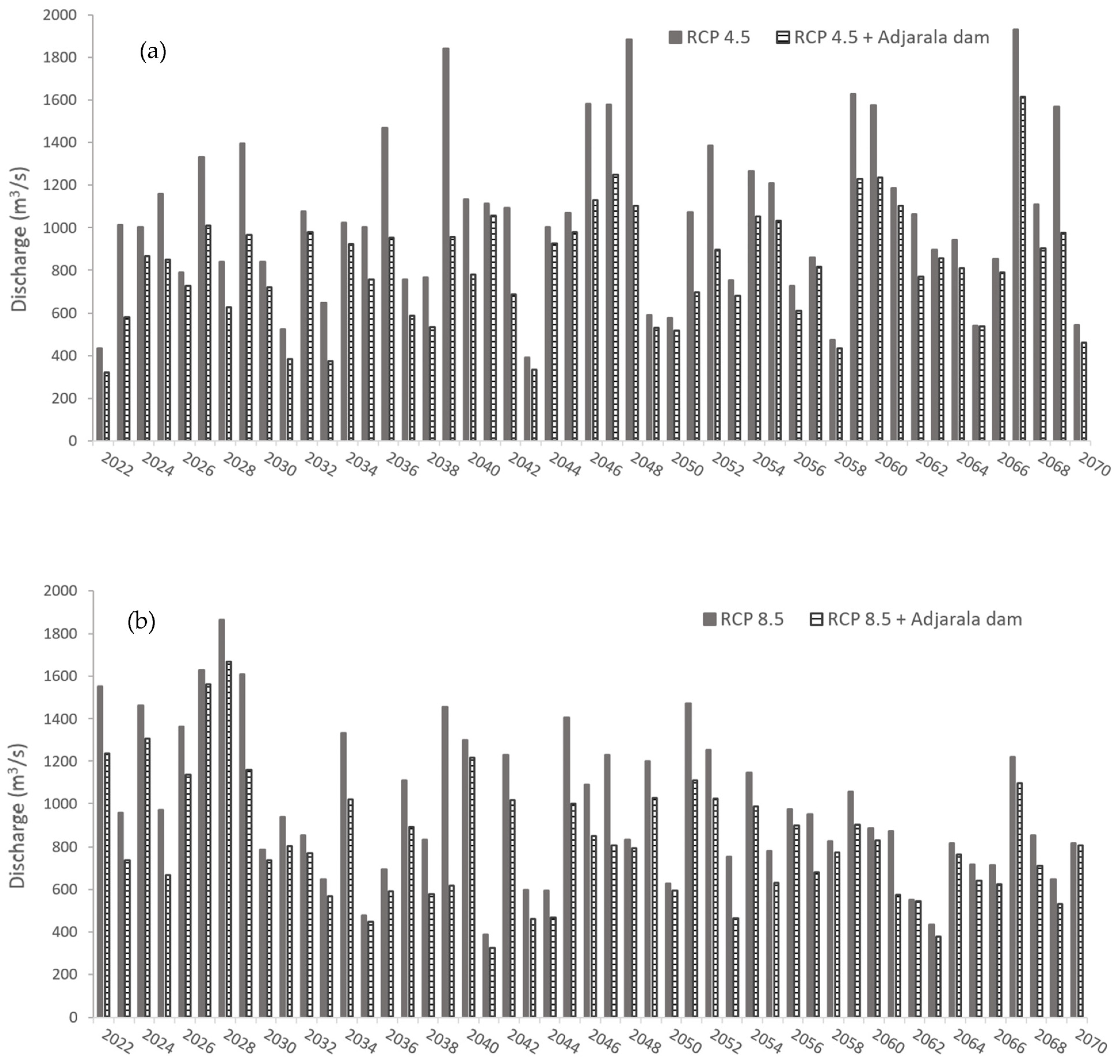
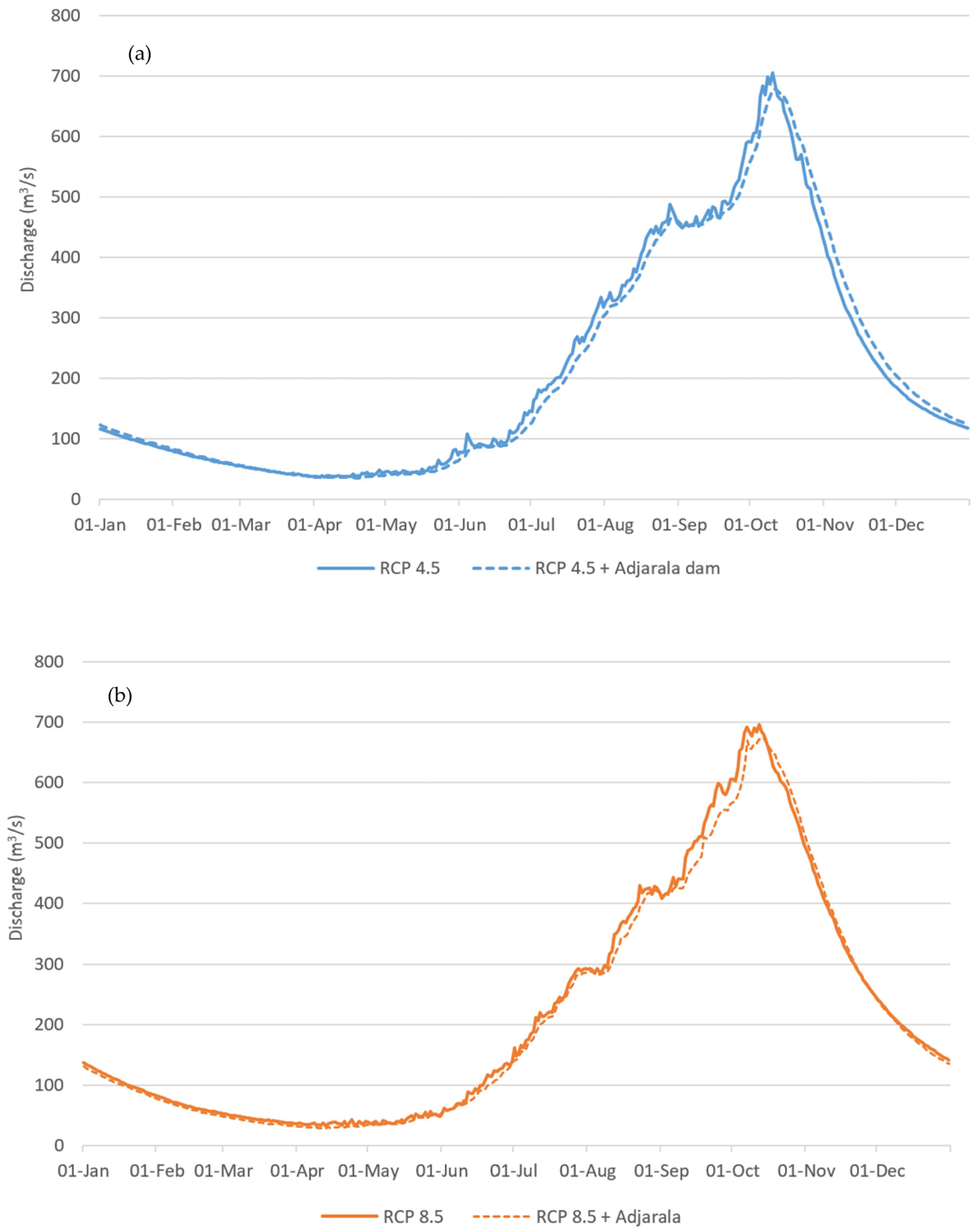
3.1.3. Effect of the Adjarala Dam

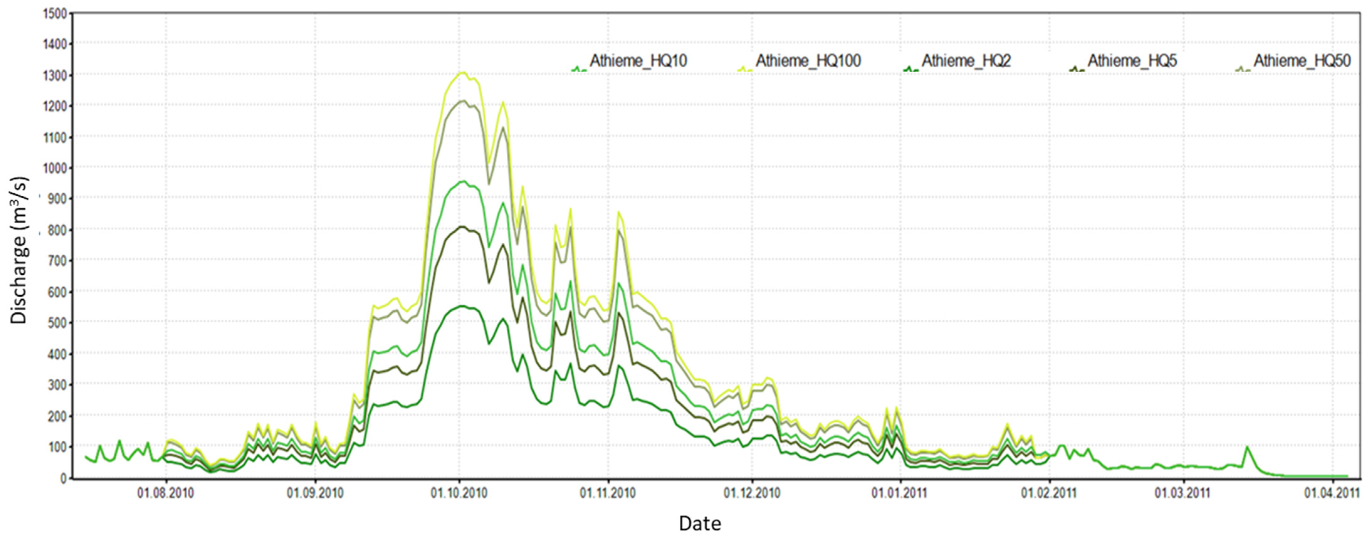
After adding the second, yet to be built, Adjarala dam into the model, the annual maxima were globally reduced (Figure 15). The average annual maximum dropped from 1050.63 m³/s to 814.42 m³/s under RCP 4.5, and from 995.29 m³/s to 816.72 m³/s under RCP 8.5.

Table 7. Return periods of runoff with climate, land-use and Adjarala dam scenarios.

	Runoff (m3/s)
Return Period	Base Case	LU + RCP		LU + RCP + Adjarala Dam
		RCP 4.5	RCP 8.5	RCP 4.5	RCP 8.5
2	554.80	1014.32	927.28	810.85	772.01
5	810.30	1373.82	1228.53	1050.35	1127.80
10	956.2	1584.36	1408.91	1173.24	1420.99
50	1218.00	1981.44	1758.66	1370.50	2279.85
100	1308.50	2125.34	1889.02	1430.94	2755.42

presents a comparison of return periods of annual maximum discharge, with and without the Adjarala dam.

The results show that constructing the Adjarala dam may reduce the recurrence of extreme discharges. Nonetheless, the peaks are expected to remain above the levels experienced to date (the base case). Under the scenario RCP 8.5, HQ50 and HQ100 are expected to increase rather a lot if the Adjarala dam is constructed. These obviously off-track values may be due to the limited length of the time series used (49 years) and to outliers.

Figure 16 presents the mean hydrographs over the period 2022–2070, with and without the Adjarala dam. The mean hydrographs indicate that, from a long-term perspective, building the Adjarala dam may reduce the discharge at Athiémé, but only slightly. This is probably attributable to the characteristics of the reservoir which might be relatively small for a substantial and long-term flood reduction under future climate- and land-use-change scenarios in the Mono catchment. In this regard, the Netherlands Commission for Environmental Assessment [27] has reported that the intended volume and surface area of the reservoir of the Adjarala dam, as announced in the dam project, might be underestimated, due to potential inaccurate elevation considerations.

The flow-duration curves (FDC) presented in Figure 17 illustrate the percentage of time that a certain amount of discharge is reached or exceeded during the period 2022–2070. The shapes of FDCs from scenarios ‘with’ and ‘without’ the Adjarala dam are similar, indicating that the overall hydrology of the flow is not expected to change. The FDCs show that peaks of 0–1% of exceedance percentage are reduced with the Adjarala dam. This supports the assumption that the dam can reduce the peak of extremely high discharges. However, a lower effect is observed for medium (20–70%) and low (70–95%) flows.

Furthermore, the very low flows (95–100% of exceedance probability) depict a remarkable decrease with the Adjarala dam, especially under the scenario RCP 8.5. This indicates that the construction of the Adjarala dam may cause the river to dry out downstream sometimes in the future. It is worth recalling that the current simulation is basically based on the storage information for the reservoir of the Adjarala dam. The reservoir simulation did not account for other water uses such as irrigation and aquaculture, as announced by the two countries [27]. The peaks might therefore become lower, and the dam more effective for flood protection, if those components were integrated. However, beyond the flood-reduction aspect tackled in this study, it is recommended that a minimum environmental flow is ensured, to sustain water availability for local communities and for ecosystem services [64,65]. As reported by King and Brown 2018 [66], the expansion of hydropower infrastructures in developing countries may jeopardize river systems and induce environmental and social impacts. Considering the potential reduction in discharge detected during very-low-flow periods, further studies on the management of the Adjarala dam, and on possible options for the regulation of the river flow, are recommended.

3.2. Flood Hazard

The flood modelling produced 25 hazard maps, modelling the return periods (HQ) 2, 5, 10, 50 and 100 of the base case, RCP 4.5 and RCP 8.5, and with the Adjarala dam. In this section, we present selected flood-hazard maps that are representative of our findings and analysis. Moreover, RCP 4.5 return periods were selected for comparison, because they show that this climate scenario produces a higher discharge when compared to RCP 8.5.

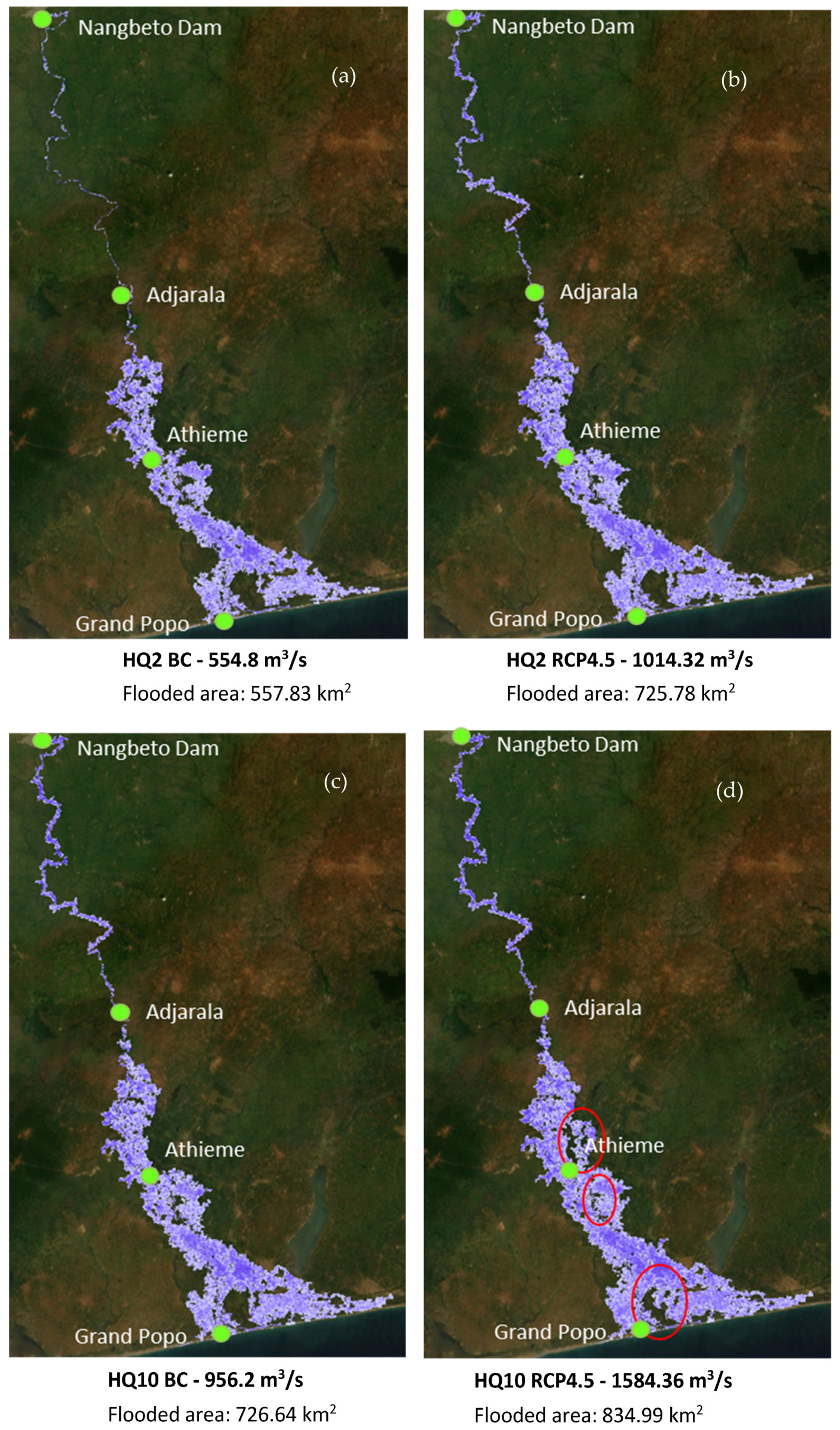
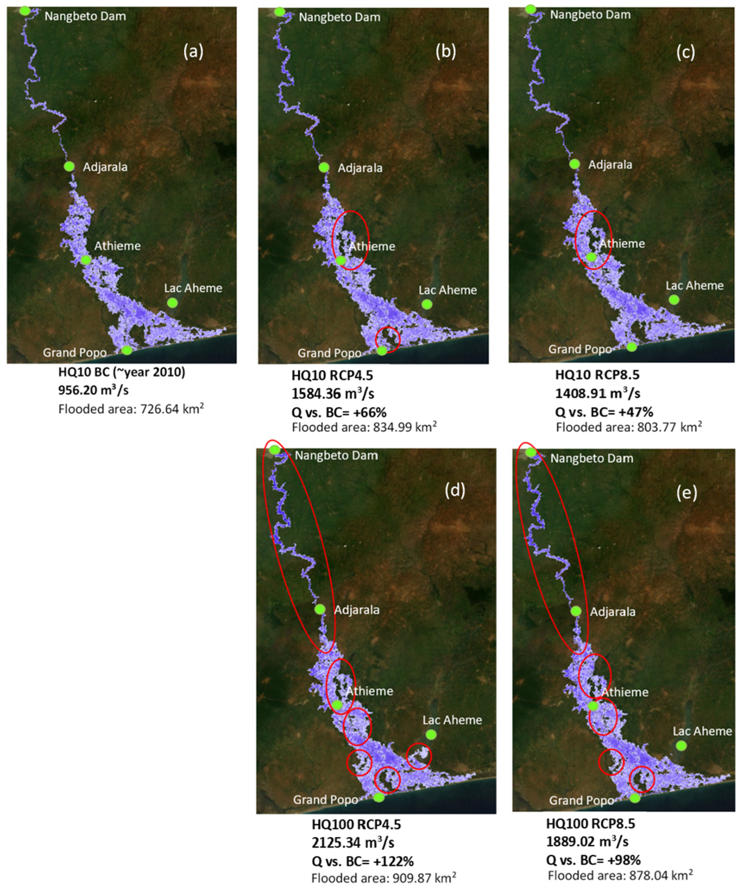
3.2.1. Base Case and RCP 4.5 (H2 and HQ10)

The findings show that flooding considerably affects, and is more dynamic, in the mid-to-downstream sections. Even with low-return periods (i.e., HQ2, with the probability of occurrence of 50% every year), many townships/communities are still affected. Figure 18 shows a comparison of the base case and RCP 4.5 HQ2 and HQ10. Looking at HQ10 RCP 4.5 (Figure 18d) which has a peak of ~600 m³/s more than the HQ10 base case (Figure 18c), large areas which have not experienced flooding in the Athiémé township and the floodplains in the south to the east of Grand Popo may be inundated. The HQ10 base case is an event comparable to the year 2010, one of the most devastating flood events recorded in the study area.

3.2.2. RCP 4.5 and RCP 8.5 (HQ10 and HQ 100)

The following figures present the scenarios RCP 4.5 and RCP 8.5 HQ10 and HQ100 with the base case. As shown again in these figures, even with an increase of >47% (HQ10 RCP 8.5) in the discharge peak of the HQ10 base case, the areas that did not experience flooding in the township of Athiémé and the southern flood plains may also be inundated (Figure 19b,c). Furthermore, an increase of >98% (Figure 20e) in the discharge peak of the HQ10 base case will also further exacerbate the flooding near the area of Lac Ahémé, in the southwest, and also the areas in the upper midsection.

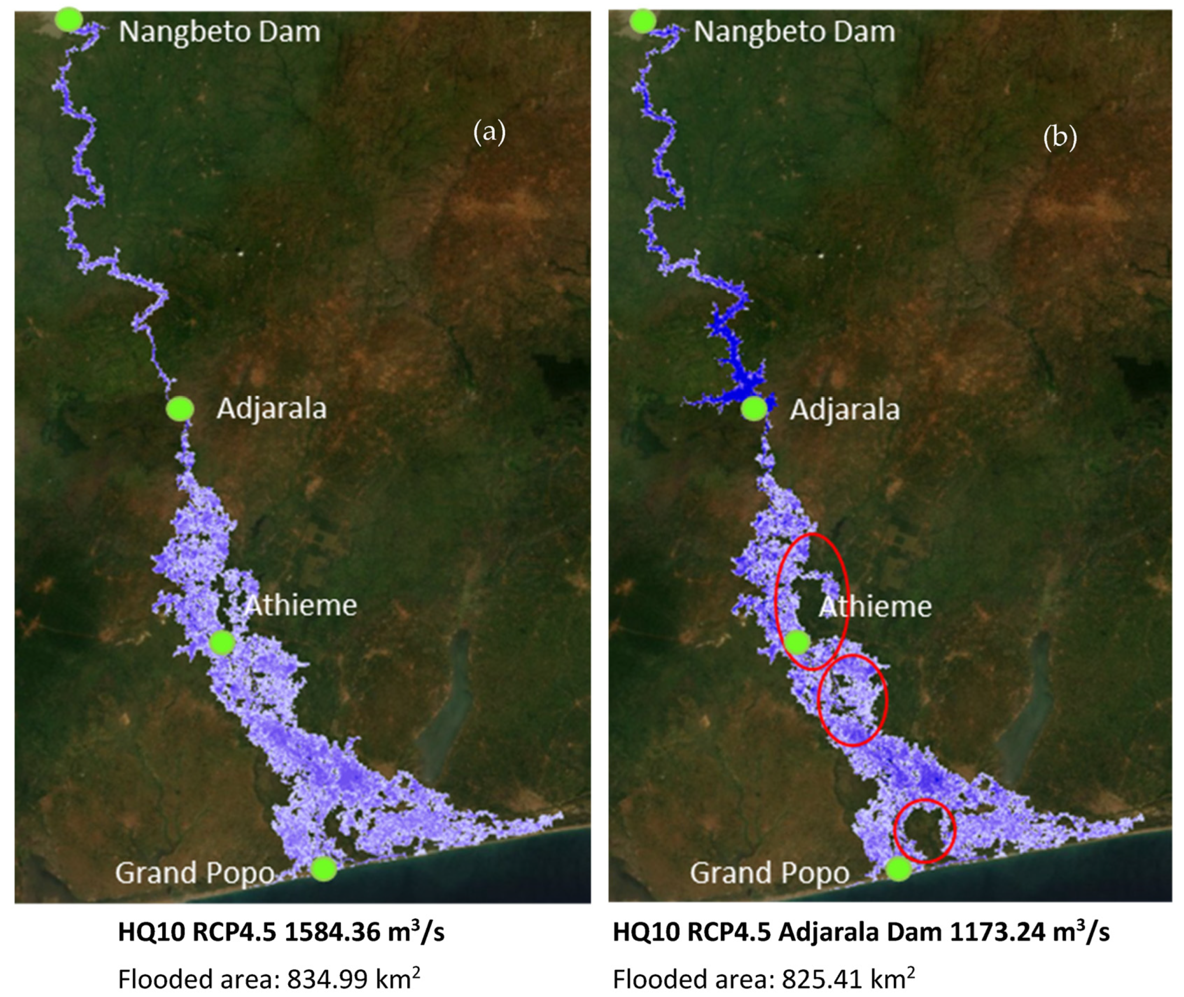
3.2.3. Effect of the Adjarala Dam on Flood Extent

Presenting the results of the Adjarala dam scenario, Figure 20 shows that for HQ10 RCP 4.5, the Adjarala dam can potentially reduce the impact of flooding. This is clearly shown in the townships of Athiémé and the southern coastal areas. The assumptions for the Adjarala dam were based on the parameters and projected operational management information provided by the Communauté Electrique du Bénin (CEB), the institution in charge of electric infrastructures in Benin and Togo [27]. This, however, can be improved if new data and information are acquired.

In addition to the findings, in Figure 21, the simulation shows that certain sections on the western coast drain the water coming from the flood plains. These existing flood plains and drains play a vital role in storage and drainage, and thus need to be preserved in order not to exacerbate flooding.

3.2.4. Limitations

The model was set up with the limited data we collected, and to compensate for this, scientifically derived inputs such as the cross-section were also used as input. If additional information and data are made available in the future, this will significantly improve the model results, especially in the southern section.

The east and west coastal area and the southeastern floodplain are beyond the scope of the basin boundary defined in this study. We tried to integrate these into the model but in our investigation the interaction here is more complex, and thus current results in the coastal area must be dealt with with caution, because of that uncertainty. This requires an in-depth investigation, integrating the other system and also (new) data regarding discharge, storm surge/tides and bathymetry. See Figure 22 below for the areas (in red) that need caution for further use.

4. Conclusions

This study assessed the combined impact of climate and land-use change on floods in the Lower Mono river catchment, and the potential effect of the forthcoming Adjarala dam. Results show that extreme flood events will persist in the future, based on the climate and LULC-change scenarios investigated. A high interannual variability of runoff is expected from 2022 to 2070, with possibilities of drought and flood occurring in consecutive years. During the wet season, more intense precipitation is expected, which translates to more extreme flood events. This is clearly seen on the mean hydrographs from 2022 to 2070, which depict higher runoff during the peak season of August–November. In addition, HQ10 events of the base case become HQ2 under the climate- and land-use-change scenarios. Although the sole investigation of land-use-change impact on flooding was not explicitly investigated here, it is already clear that urban growth will also exacerbate flooding, producing higher runoffs. This will have an increased impact on communities and the agricultural economy, which is the main economic activity in the study area. The Adjarala dam may reduce the magnitude of extreme flood events in the future. However, it may also affect water availability during low-flow periods, and thus jeopardize environmental flow and related benefits in the LMR basin. Based on the observed variability of spatio-temporal impacts on flood hazard in the LMR basin, both local and basin scales need to be taken into account by decision makers. The expansion of settlements in flooded areas that are currently not settled should be avoided. The integrated and participatory approach used in this study, with the engagement of stakeholders for flood-map validation, should be maintained and furthered for the identification of sustainable adaptation measures. Further studies could investigate the capabilities of other models for flood-hazard mapping in the LMR basin. In addition, improved model performances may be achieved with more in situ data, e.g., longer discharge-time series, measured cross-sections of the river, and tidal data. Furthermore, a system analysis of floods, involving water intrusion from the sea and the influence of the nearby Ahémé lake are recommended, in order to obtain a holistic perspective of flood hazards in the LMR basin. Finally, vulnerability and risk assessments are recommended for an effective preparedness, response and adaptation to floods in the LMR basin.

References

1. Vivekananda, J. Why Climate Change Matters for Human Security; International Development Research Centre (IDRC): Ottawa, ON, Canada, 2022. [Google Scholar]
2. Adger, W.N.; Pulhin, J.M.; Barnett, J.; Dabelko, G.D.; Hovelsrud, G.K.; Levy, M.; Spring, Ú.O.; Vogel, C.H. Human Security. In Climate Change 2014: Impacts, Adaptation, and Vulnerability; Part A: Global and Sectoral Aspects; Contribution of Working Group II to the Fifth Assessment Report of the Intergovernmental Panel on Climate Change; Field, C.B., Barros, V.R., Dokken, D.J., Mach, K.J., Mastrandrea, M.D., Bilir, T.E., Chatterjee, M., Ebi, K.L., Estrada, Y.O., Genova, R.C., et al., Eds.; Cambridge University Press: Cambridge, UK; New York, NY, USA, 2014; pp. 755–791. [Google Scholar]
3. Trisos, C.H.; Adelekan, I.O.; Totin, E.; Ayanlade, A.; Efitre, J.; Gemeda, A.; Kalaba, K.; Lennard, C.; Masao, C.; Mgaya, Y.; et al. Africa. In Climate Change 2022: Impacts, Adaptation and Vulnerability; Contribution of Working Group II to the Sixth Assessment Report of the Intergovernmental Panel on Climate Change; Pörtner, H.-O., Roberts, D.C., Tignor, M., Poloczanska, E.S., Mintenbeck, K., Alegría, A., Craig, M., Langsdorf, S., Löschke, S., Möller, V., et al., Eds.; Cambridge University Press: Cambridge, UK; New York, NY, USA, 2022; pp. 1285–1455. ISBN 9781009325844. [Google Scholar]
4. Potapov, P.; Hansen, M.C.; Pickens, A.; Hernandez-Serna, A.; Tyukavina, A.; Turubanova, S.; Zalles, V.; Li, X.; Khan, A.; Stolle, F.; et al. The Global 2000–2020 Land Cover and Land Use Change Dataset Derived From the Landsat Archive: First Results. Front. Remote Sens. 2022, 3, 18. [Google Scholar] [CrossRef]
5. Piao, S.; Friedlingstein, P.; Ciais, P.; de Noblet-ducoudre, N.; Labat, D.; Zaehle, S. Changes in Climate and Land Use Have a Larger Direct Impact than Rising CO2 on Global River Runoff Trends. Proc. Natl. Acad. Sci. USA 2007, 104, 15242–15247. [Google Scholar] [CrossRef] [Green Version]
6. Collins, M.; Knutti, R.; Arblaster, J.; Dufresne, J.-L.; Fichefet, T.; Friedlingstein, P.; Gao, X.; Gutowski, W.J.; Johns, T.; Krinne, G.; et al. Long-Term Climate Change: Projections, Commitments and Irreversibility. In Climate Change 2013: The Physical Science Basis; Contribution of Working Group I to the Fifth Assessment Report of the Intergovernmental Panel on Climate Change; Stocker, T.F., Qin, D., Plattner, G.-K., Tignor, M., Allen, S.K., Boschung, J., Nauels, A., Xia, Y., Bex, V., Midgley, P.M., Eds.; Cambridge University Press: Cambridge, UK; New York, NY, USA, 2013; pp. 1029–1136. [Google Scholar]
7. Masson-Delmotte, V.; Zhai, P.; Pirani, A.; Connors, S.L.; Péan, C.; Berger, S.; Caud, N.; Chen, Y.; Goldfarb, L.; Gomis, M.I.; et al. (Eds.) IPCC Summary for Policymakers. In Climate Change 2021: The Physical Science Basis. Contribution of Working Group I to the Sixth Assessment Report of the Intergovernmental Panel on Climate Change; Cambridge University Press: Cambridge, UK; New York, NY, USA, 2021; pp. 3–32. [Google Scholar]
8. Barry, A.A.; Caesar, J.; Tank, A.M.G.K.; Aguilar, E.; Mcsweeney, C.; Ahmed, M.; Nikiema, M.P.; Narcisse, K.B.; Sima, F.; Stafford, G.; et al. West Africa Climate Extremes and Climate Change Indices. Int. J. Climatol. 2018, 38, 921–938. [Google Scholar] [CrossRef]
9. Callaghan, M.; Schleussner, C.; Nath, S.; Lejeune, Q.; Knutson, T.R.; Reichstein, M.; Hansen, G.; Theokritoff, E.; Andrijevic, M.; Brecha, R.J.; et al. Machine-Learning-Based Evidence and Attribution Mapping of 100,000 Climate Impact Studies. Nat. Clim. Chang. 2021, 11, 966–972. [Google Scholar] [CrossRef]
10. Maidment, R.I.; Allan, R.P.; Black, E. Recent Observed and Simulated Changes in Precipitation over Africa. Geophys. Res. Lett. 2015, 42, 8155–8164. [Google Scholar] [CrossRef]
11. Pechlivanidis, I.G.; Arheimer, B.; Donnelly, C.; Hundecha, Y.; Huang, S.; Aich, V.; Samaniego, L.; Eisner, S.; Shi, P. Analysis of Hydrological Extremes at Different Hydro-Climatic Regimes under Present and Future Conditions. Clim. Change 2017, 141, 467–481. [Google Scholar] [CrossRef] [Green Version]
12. Moges, E.; Demissie, Y.; Larsen, L.; Yassin, F. Review: Sources of Hydrological Model Uncertainties and Advances in Their Analysis. Water 2021, 18, 28. [Google Scholar] [CrossRef]
13. UNDP. Evaluation des Dommages, Pertes et Besoins de Reconstruction Post Catastrophes des Inondations de 2010 au Togo; UNDP: Lomé, Togo, 2010. [Google Scholar]
14. World Bank; United Nations Development Programme. Inondations au Bénin: Rapport d’Évaluation des Besoins Post Catastrophe; UNDP: Cotonou, Benin, 2011. [Google Scholar]
15. Amoussou, E. Variabilité Pluviométrique et Dynamique Hydro-Sédimentaire Du Bassin Versant Du Complexe Lagunaire Mono-Ahémé-Couffo (Afrique de l’Ouest). Ph.D. Thesis, Université de Bourgogne, Dijon, France, 2010. [Google Scholar]
16. Lawin, E.; Lamboni, B.; Manirakiza, C.; Kamou, H. Future Extremes Temperature: Trends and Changes Assessment over the Mono River Basin, Togo (West Africa). J. Water Resour. Prot. 2019, 11, 82–98. [Google Scholar] [CrossRef] [Green Version]
17. Kissi, A.E.; Abbey, G.A.; Agboka, K.; Egbendewe, A. Quantitative Assessment of Vulnerability to Flood Hazards in Downstream Area of Mono Basin, South-Eastern Togo: Yoto District. J. Geogr. Inf. Syst. 2015, 7, 607–619. [Google Scholar] [CrossRef] [Green Version]
18. Ntajal, J.; Lamptey, B.L.; Sogbedji, M.J.; Wilson-Bahun, K.K. Rainfall Trends and Flood Frequency Analyses in the Lower Mono River Basin in Togo, West Africa. Int. J. Adv. Res. 2016, 4, 10. [Google Scholar]
19. Houngue, N.R.; Almoradie, A.D.S.; Evers, M. A Multi Criteria Decision Analysis Approach for Regional Climate Model Selection and Future Climate Assessment in the Mono River Basin, Benin and Togo. Atmosphere 2022, 13, 1471. [Google Scholar] [CrossRef]
20. Amoussou, E.; Awoye, H.; Vodounon, H.S.T.; Obahoundje, S.; Camberlin, P.; Diedhiou, A.; Kouadio, K.; Mahé, G.; Houndénou, C.; Boko, M. Climate and Extreme Rainfall Events in the Mono River Basin (West Africa): Investigating Future Changes with Regional Climate Models. Water 2020, 12, 833. [Google Scholar] [CrossRef] [Green Version]
21. Batablinle, L.; Lawin, E.; Agnide, S.; Celestin, M. Africa-Cordex Simulations Projection of Future Temperature, Precipitation, Frequency and Intensity Indices over Mono Basin in West Africa. J. Earth Sci. Clim. Change 2018, 9, 490. [Google Scholar] [CrossRef]
22. Batablinlè, L.; Agnidé, E.L.; Celestin, M.; Zakari, M.D. Variability of Future Rainfall over the Mono River Basin of West-Africa. Am. J. Clim. Change 2019, 8, 137–155. [Google Scholar] [CrossRef] [Green Version]
23. Koubodana, H.D.; Adounkpe, J.; Tall, M.; Amoussou, E.; Atchonouglo, K.; Mumtaz, M. Trend Analysis of Hydro-Climatic Historical Data and Future Scenarios of Climate Extreme Indices over Mono River Basin in West Africa. Am. J. Rural Dev. 2020, 8, 37–52. [Google Scholar]
24. Lawin, E.; Hounguè, N.R.; Biaou, C.A.; Badou, D.F. Statistical Analysis of Recent and Future Rainfall and Temperature Variability in the Mono River Watershed (Benin, Togo). Climate 2019, 7, 8. [Google Scholar] [CrossRef] [Green Version]
25. Koubodana, D.H.; Diekkrüger, B.; Näschen, K.; Adounkpè, J.; Atchonouglo, K. Impact of the Accuracy of Land Cover Data Sets on the Accuracy of Land Cover Change Scenarios in the Mono River Basin, Togo, West Africa. Int. J. Adv. Remote Sens. GIS 2019, 8, 3073–3095. [Google Scholar] [CrossRef]
26. Thiam, S.; Salas, E.A.L.; Houngue, N.R.; Almoradie, D.A.S.; Verleysdonk, S.; Adounkpe, J.G.; Komi, K. Modelling Land Use and Land Cover in the Transboundary Mono River Catchment of Togo and Benin Using Markov Chain and Stakeholder’s Perspectives. Sustainability 2022, 14, 4160. [Google Scholar] [CrossRef]
27. CNEE. Barrage Hydroélectrique d’Adjarala. In Avis Sur L’examen de Qualité de l’EIES; CNEE: Marknesse, The Netherlands, 2014. [Google Scholar]
28. Hargreaves, G.H.; Samani, Z. Reference Crop Evapotranspiration from Ambient Air Temperature. In Proceedings of the Winter Meeting American Society of Agricultural Engineers; American Society of Agricultural Engineers: Chicago, IL, USA, 1985; pp. 1–13. [Google Scholar]
29. Koubodana, H.D.; Adounkpe, J.G.; Atchonouglo, K.; Djaman, K.; Larbi, I.; Lombo, Y.; Kpemoua, K.E. Modelling of Streamflow before and after Dam Construction in the Mono River Basin in Togo- Benin, West Africa. Intl. J. River Basin Manag. 2021, 1, 1–17. [Google Scholar] [CrossRef]
30. Amoussou, E. Analyse Hydrométéorologique des Crues Dans Le Bassin-Versant Du Mono En Afrique de l’Ouest Avec Un Modèle Conceptuel Pluie-Débit; FMSH-WP-2014; Fondation Maison des Sciences de l’Homme: Paris, France, 2015. [Google Scholar]
31. Poméon, T.; Diekkrüger, B.; Springer, A.; Kusche, J.; Eicker, A. Multi-Objective Validation of SWAT for Sparsely-Gauged West African River Basins—A Remote Sensing Approach Thomas. Water 2018, 10, 451. [Google Scholar] [CrossRef] [Green Version]
32. Droogers, P.; Allen, R.G. Estimating Reference Evapotranspiration under Inaccurate Data Conditions. Irrig. Drain. Syst. 2002, 16, 33–45. [Google Scholar] [CrossRef]
33. Hargreaves, G.H.; Allen, R.G. History and Evaluation of Hargreaves Evapotranspiration Equation. J. Irrig. Drain. Eng. 2003, 129, 53–63. [Google Scholar] [CrossRef]
34. IUSS Working Group WRB. World Reference Base for Soil Resources 2006, 2nd ed.; FAO: Rome, Italy, 2006; ISBN 9251055114. [Google Scholar]
35. Laplante, L. Etude Pédologique Du Comté de Bagot; Ministère de L’agriculture, Division des Sols: Québec, Canada, 1959.
36. Houessou, S. Les Inondations et Les Risques Previsionnels Liés Aux Barrages Hydroelectriques. Ph.D. Thesis, Université d’Abomey-Calavi, Abomey-Calavi, Benin, 2016. [Google Scholar]
37. Arnold, J.G.; Kiniry, J.R.; Srinivasan, R.; Williams, J.R.; Haney, E.B.; Neitsch, S.L. Soil & Water Assessment Tool. Input/Output Documentation; Version 2012; Texas Water Resources Institute: College Station, TX, USA, 2012; Available online: http://swat.tamu.edu/media/69296/SWAT-IO-Documentation-2012.pdf (accessed on 10 January 2023).
38. Schuol, J.; Abbaspour, K.C. Calibration and Uncertainty Issues of a Hydrological Model (SWAT) Applied to West Africa. Adv. Geosci. 2006, 9, 137–143. [Google Scholar] [CrossRef] [Green Version]
39. Begou, J.C.; Jomaa, S.; Benabdallah, S.; Bazie, P.; Afouda, A.; Rode, M. Multi-Site Validation of the SWAT Model on the Bani Catchment: Model Performance and Predictive Uncertainty. Water 2016, 8, 178. [Google Scholar] [CrossRef]
40. Badou, D.F.; Diekkrüger, B.; Kapangaziwiri, E.; Mbaye, M.L.; Yira, Y.; Lawin, E.A.; Oyerinde, G.T.; Afouda, A. Modelling Blue and Green Water Availability under Climate Change in the Beninese Basin of the Niger River Basin, West Africa. Hydrol. Process. 2018, 32, 2526–2542. [Google Scholar] [CrossRef]
41. Awotwi, A.; Kumi, M.; Pe, J.; Yeboah, F.; Ik, N. Earth Science & Climatic Change Predicting Hydrological Response to Climate Change in the White Volta. J. Earth Sci. Clim. Change 2015, 6, 249. [Google Scholar] [CrossRef]
42. Ampofo, S.; Gyekye, E.; Ampadu, B.; Sackey, I. Modelling Soil and Water Dynamics in the Black Volta Basin Using the Soil and Water Assessment Tool (SWAT) Model. Ghana J. Sci. Technol. Dev. 2021, 7, 44–57. [Google Scholar] [CrossRef]
43. Bossa, A.Y.; Diekkrüger, B.; Agbossou, E.K. Scenario-Based Impacts of Land Use and Climate Change on Land and Water Degradation from the Meso to Regional Scale. Water 2014, 6, 3152–3181. [Google Scholar] [CrossRef] [Green Version]
44. Hounkpè, B.Y.J.; Diekkrüger, B.; Badou, D.F.; Bossa, A.Y.; Lawin, E.A.; Adounkpè, J.; Afouda, A.A. How Does Climate and Land Use Change Influence Flood Hazard in Benin? In Regional Climate Change Series: Floods; WASCAL Publishing: Kansas, MI, USA, 2019; pp. 44–49. [Google Scholar]
45. Adnan, M.; Kang, S.; Zhang, G.; Saifullah, M.; Anjum, M.N.; Ali, A.F. Simulation and Analysis of the Water Balance of the Nam Co Lake Using SWAT Model. Water 2019, 11, 1383. [Google Scholar] [CrossRef] [Green Version]
46. Abbaspour, K.C. SWAT-CUP SWAT Calibration and Uncertainty Programs—A User Manual; Swiss Federal Institute of Aquatic Science and Technology: Duebendorf, Switzerland, 2015. [Google Scholar]
47. Abbaspour, K. SWATCUP “How to Do”: Validation. Available online: https://www.youtube.com/watch?v=7E9qxRzwmV4 (accessed on 30 November 2022).
48. Hounkpe, J. Assessing the Climate and Land Use Changes Impact on Flood Hazard in Ouémé River Basin, Benin (West Africa). Ph.D. Thesis, University of Abomey-Calavi, Abomey-Calavi, Benin, 2016. [Google Scholar]
49. Schuol, J.; Abbaspour, K.C.; Srinivasan, R.; Yang, H. Estimation of Freshwater Availability in the West African Sub-Continent Using the SWAT Hydrologic Model. J. Hydrol. 2008, 352, 30–49. [Google Scholar] [CrossRef]
50. Schuol, J.; Abbaspour, K.C.; Yang, H.; Srinivasan, R.; Zehnder, A.J.B. Modeling Blue and Green Water Availability in Africa. Water Resour. Res. 2008, 44, 212–221. [Google Scholar] [CrossRef] [Green Version]
51. Gupta, H.V.; Kling, H.; Yilmaz, K.K.; Martinez, G.F. Decomposition of the Mean Squared Error and NSE Performance Criteria: Implications for Improving Hydrological Modelling. J. Hydrol. 2009, 377, 80–91. [Google Scholar] [CrossRef] [Green Version]
52. Mann, H.B. Non-Parametric Test against Trend. Econometrica 1945, 13, 245–259. [Google Scholar] [CrossRef]
53. Vogel, M.R.; Fennessey, N.M. Flow-Duration Curves. New Interpretation and Confidence Intervals. J. Water Resour. Plan. Manag. 1994, 120, 485–504. [Google Scholar] [CrossRef]
54. Berhanu, B.; Seleshi, Y.; Demisse, S.S.; Melesse, A.M. Flow Regime Classification and Hydrological Characterization: A Case Study of Ethiopian Rivers. Water 2015, 7, 3149–3165. [Google Scholar] [CrossRef] [Green Version]
55. Searcy, J. Flow-Duration Curves. In Manual of Hydrology: Part 2. Low-Flow Techniques; Hickel, W.J., Ed.; United States Government Printing Office: Washington, DC, USA, 1959. [Google Scholar]
56. Gordon, N.D.; Mcmahon, T.A.; Finlayson, B.L.; Gippel, C.J.; Nathan, R.J. Stream Hydrology: An Introduction for Ecologists, 2nd ed.; John Wiley: Chichester, UK, 2004; ISBN 0470843578. [Google Scholar]
57. Icyimpaye, G.; Abdelbaki, C.; Mourad, K.A. Hydrological and Hydraulic Model for Flood Forecasting in Rwanda. Model. Earth Syst. Environ. 2022, 8, 1179–1189. [Google Scholar] [CrossRef]
58. Komi, K.; Neal, J.; Trigg, M.A.; Diekkrüger, B. Modelling of Flood Hazard Extent in Data Sparse Areas: A Case Study of the Oti River Basin, West Africa. J. Hydrol. Reg. Stud. 2017, 10, 122–132. [Google Scholar] [CrossRef] [Green Version]
59. Mitsopoulos, G.; Panagiotatou, E.; Sant, V.; Baltas, E.; Diakakis, M.; Lekkas, E.; Stamou, A. Optimizing the Performance of Coupled 1D/2D Hydrodynamic Models for Early Warning of Flash Floods. Water 2022, 14, 2356. [Google Scholar] [CrossRef]
60. Chow, V.T. Open-Channel Hydraulics; McGraw-Hill Book Co.: New York, NY, USA, 1959; p. 680. [Google Scholar]
61. Millington, N.; Das, S.; Simonovic, S.P. The Comparison of GEV, Log-Pearson Type 3 and Gumbel Distributions in the Upper Thames River Watershed under Global Climate Models; Department of Civil and Environmental Engineering, The University of Western Ontario: London, ON, Canada, 2011. [Google Scholar]
62. Nicholson, S.E. The West African Sahel: A Review of Recent Studies on the Rainfall Regime and Its Interannual Variability. ISRN Meteorol. 2013, 2013, 453521. [Google Scholar] [CrossRef]
63. Wetzel, M.; Schudel, L.; Almoradie, A.; Komi, K.; Adounkpè, J.; Walz, Y.; Hagenlocher, M. Assessing Flood Risk Dynamics in Data-Scarce Environments—Experiences from Combining Impact Chains with Bayesian Network Analysis in the Lower Mono River Basin, Benin. Front. Water 2022, 4, 16. [Google Scholar] [CrossRef]
64. IUCN. The Essentials of Environmental Flows; Dyson, M., Bergkamp, G., Scanlon, J., Eds.; IUCN Publications Services Unit: Gland, Switzerland; Cambridge, UK, 2003; ISBN 2831707250. [Google Scholar]
65. WMO. Guidance on Environmental Flows. In Integrating E-Flow Science with Fluvial Geomorphology to Maintain Ecosystem Services; World Meteorological Organization (WMO): Geneva, Switzerland, 2019; ISBN 9789263112354. [Google Scholar]
66. King, J.M.; Brown, C. Environmental Flow Assessments Are Not Realizing Their Potential as an Aid to Basin Planning. Front. Environ. Sci. Receiv. 2018, 6, 113. [Google Scholar] [CrossRef]
Figure 1. Study area location.
Sustainability 15 05862 g001
Figure 2. LULC maps of the Mono River basin (Thiam et al., 2022 [26]).
Sustainability 15 05862 g002
Figure 3. Soil map.
Sustainability 15 05862 g003
Figure 6. Lower Mono River (LMR) basin study area showing the modelled sections and water level measuring stations in green markers.
Sustainability 15 05862 g006
Figure 7. Hydrograph of Athiémé station—2010 event.
Sustainability 15 05862 g007
Figure 8. Model results verification.
Sustainability 15 05862 g008
Figure 9. Base Case (HQ) for different stations.
Sustainability 15 05862 g009
Figure 10. Base-Case-HQ-derived hydrograph for Athiémé station.
Sustainability 15 05862 g010
Figure 11. Observation and 95PPU of the simulation during (a) calibration and (b) validation.
Sustainability 15 05862 g011
Figure 12. Daily runoff under climate- and land-use-change scenarios.
Sustainability 15 05862 g012
Figure 13. Past and future mean hydrographs.
Sustainability 15 05862 g013
Figure 14. Boxplots of discharge with scenarios (a) RCP 4.5 and (b) RCP 8.5.
Sustainability 15 05862 g014
Figure 15. Annual maximum discharge from 2022 to 2070 under (a) RCP 4.5 and (b) RCP 8.5.
Sustainability 15 05862 g015
Figure 16. Mean hydrograph 2022–2070 under scenarios (a) RCP 4.5 and (b) RCP 8.5, with and without the Adjarala dam.
Sustainability 15 05862 g016
Figure 17. Flow-duration curves (FDCs) with and without the Adjarala dam under scenarios (a) RCP 4.5 and (b) RCP 8.5.
Sustainability 15 05862 g017
Figure 18. Flood-hazard maps—(ad) presents the base case and RCP 4.5 scenarios of return periods 2 and 10 (HQ2 and HQ10). The red circles shown in (d) are new areas inundated with higher discharges.
Sustainability 15 05862 g018
Figure 19. Flood-hazard maps—(ae) presents RCP 4.5 vs. RCP 8.5 (HQ10 and HQ100) scenarios. The red circles are new areas inundated with higher discharges.
Sustainability 15 05862 g019
Figure 20. Flood-hazard map—RCP 4.5—(b) with and (a) without Adjarala Dam. The red circles are new areas inundated with higher discharges.
Sustainability 15 05862 g020
Figure 21. Flood-hazard maps—Western coast drainage. The green circles are drainage areas.
Sustainability 15 05862 g021
Figure 22. Modelled area for further investigation.
Sustainability 15 05862 g022