Seismic Signal Characteristics and Numerical Modeling Analysis of the Xinmo Landslide

Abstract

Due to the high elevation and huge potential energy of high-level landslides, they are extremely destructive and have prominent kinetic-hazard effects. Studying the kinetic-hazard effects of high-level landslides is very important for landslide risk prevention and control. In this paper, we focus on the high-level landslide that occurred in Xinmo on 24 June 2017. The research is carried out based on a field geological survey, seismic signal analysis, and the discrete element method. Through ensemble empirical mode decomposition (EEMD) and Fourier transformation, it is found that the seismic signals of the Xinmo landslide are mainly located at low frequencies of 0–10 Hz, and the dominant frequency range is 2–8 Hz. In addition, the signal time-frequency analysis and numerical simulation calculation results reveal that the average movement distance of the sliding body was about 2750 m, and the average movement speed was about 22.9 m/s. The movement process can be divided into four main stages: rapid start, impact loading, fragmentation and migration, and scattered accumulation stages. We also provide corresponding suggestions for the zoning of high-level landslide geological hazards.

1. Introduction

Landslides have the characteristics of a fast movement speed, wide range of disasters, and strong destructive power. These features are more pronounced for high-level landslides in alpine and canyon regions [1,2,3,4]. High-level landslides are difficult to witness and record on video due to the high altitudes of their source areas and their fast movement processes [5,6]. At present, the inverse analysis of the disaster process of high-level landslides has mainly been carried out through analysis of the seismic signals generated by such landslides, numerical simulation, and field geological surveys [7,8]. These methods can effectively reveal the landslide movement behavior and finally realize the inverse analysis of the disaster-forming mechanism of the landslide [9,10].

In the analysis of high-level landslide disasters, the seismic signals of such landslides can completely record the entire movement process. The change in the signal amplitude can be used to divide the landslide process into stages, to calculate the change in the movement speed, to determine the destructive strength, and to estimate the speed and movement distance [11,12]. Since landslides mostly occur in remote mountainous areas, the collection of seismic signals is mainly affected by the distribution of the seismic stations. Generally, only large-scale landslide vibration signals are relatively easy to obtain. This is because landslide vibration signals have a smaller distribution of high and low frequency ranges and a smaller vibration amplitude range than conventional seismic signals, and stronger landslide vibration signals are relatively easier to identify and analyze [13,14]. Therefore, the analysis and identification of landslide vibration signals is one of the main factors restricting the study of landslide seismology [15,16]. At present, in the analysis of landslide kinetic disasters, numerical simulation is another important means of landslide disaster analysis, and the movement parameters that can be obtained mainly include the maximum movement speed, the farthest movement distance, and the thickness of the accumulation body [17,18]. These results can be compared with and verified using seismic analysis results. The results of such studies can provide important references for engineering design and layouts for the prevention and control of landslides [19,20]. Currently, the combined use of landslide seismology and numerical simulation analysis in landslide disaster research has been gradually popularized and has produced good results [21].

The Xinmo landslide is a typical example of the high-level landslide geological disasters that have occurred in the alpine and canyon regions in southwestern China in recent years, providing samples for the study of landslide kinetic disasters [22]. The research on the Xinmo landslide has mainly focused on analysis of the landslide-inducing geological mechanism, the disaster evolution process, and the dynamic process [23,24,25,26]. In this study, based on the above-mentioned existing studies, the spectral characteristics of the Xinmo landslide were analyzed using the ensemble empirical mode decomposition (EEMD) method and fast Fourier transformation. The stages of the landslide movement were preliminarily divided via time-frequency signal analysis and ere compared with the landslide movement process calculated using the discrete element method. Finally, the high-level landslide disaster partition method was investigated. The results of this study provide a reference for high-level landslide kinetic research.

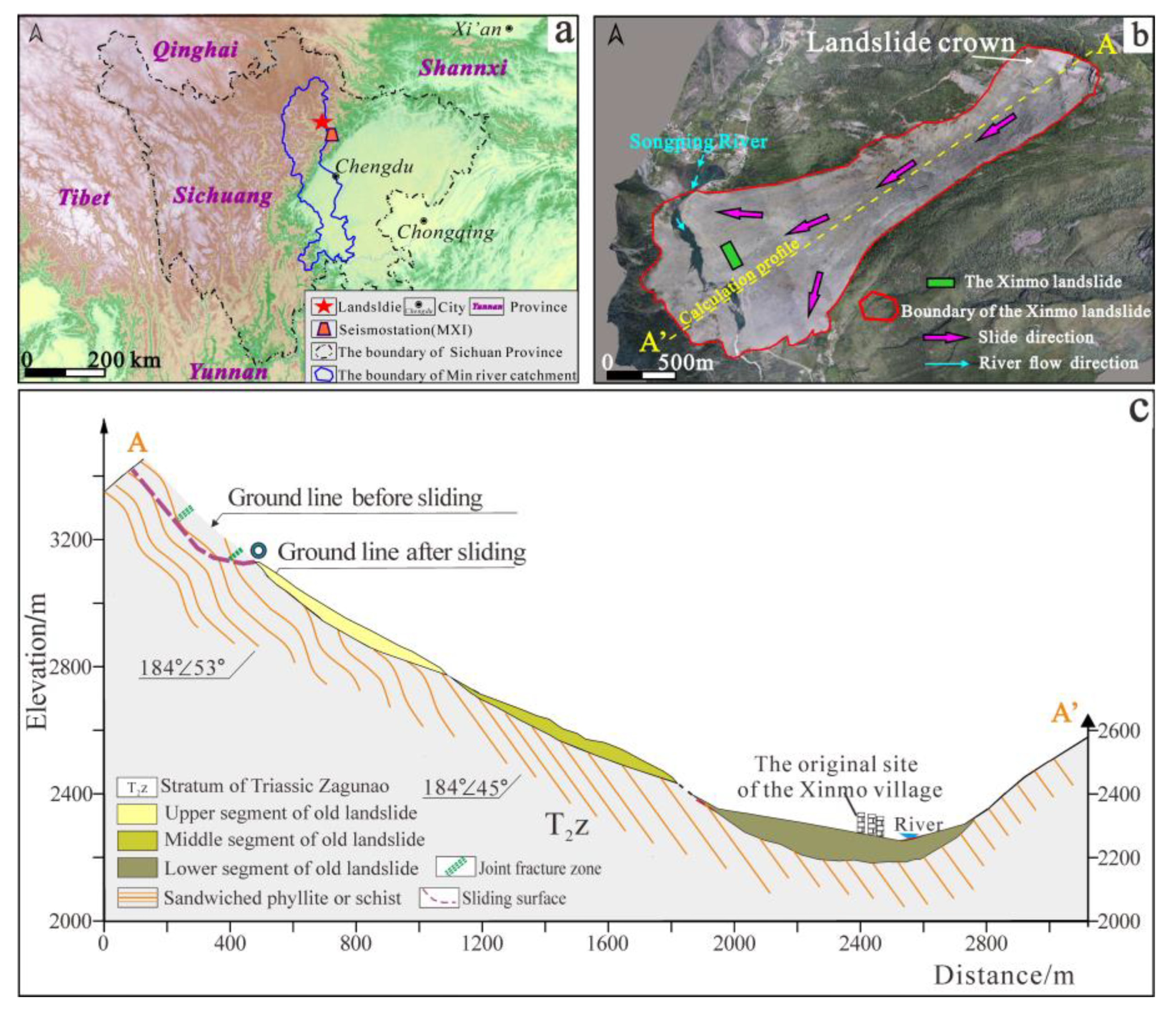
2. Site Overview

2.1. Landslide Event

At 05:39 on 24 June 2017, a super-large high-level consequent bedding rockslide occurred on Fugui Mountain. Xinmo Village in Songpinggou, Mao County, Sichuan Province, was buried and 83 people were killed (Figure 1a,b). The trailing edge of the Xinmo landslide was located on the ridged top of Fugui Mountain, which was covered with dense vegetation. The elevation of the trailing edge was 3450 m, the elevation of the leading edge was about 2250 m, and the height difference was about 1200 m. The horizontal movement distance was up to 2850 m, and the volume of the entire landslide accumulation was about 1.59 × 10⁷ m³ (Figure 1c). The Xinmo landslide is located at the intersection of the Songpinggou fault zone and the Minjiang fault zone. Affected by the continuous reverse movement of the fault zone, the Fugui mountain body exhibits an upward uplift trend, which aggravates the concealment of the disaster development of the Xinmo landslide. In addition, the tensile stress of the ridge mountain is concentrated, and the fracture development in the slip source area is aggravated. There are two sets of anti-dip slip fracture zones with widths of about 5–10 m in the sliding source area, which provide the dominant weak surface for the bulging deformation and sliding shear of the rock mass. In addition, on the surface of the slope, there are old residual landslide deposits triggered by the 1933 Diexi Ms7.5 earthquake and old landslide deposits composed of inverted debris cones formed by the upper gravity in the later period. The average thickness is about 20 m, and it is composed of upper, middle, and lower sections, with a total volume of about 873.6 × 10⁴ m³ (Figure 1c). The exposed strata are mainly the meta-morphic quartz sandstone and splint rock of the Zagunao Formation. Several studies have shown that the rock of Fugui Mountain on the left bank of Songpinggou in the Minjiang River Basin, where the Xinmo landslide occurred, has developed a fragmented-scattered structure under earthquake activity [27,28]. Under the influence of long-term rainfall, the landslide mass of about 500 × 10⁴ m³ started to undergo shearing at a high elevation. Under the action of the gravitational potential energy, a continuously impact load was applied to the upper part of the loose accumulation body of the old landslide, resulting in destabilization and reactivation of the loose accumulation body. During the movement process, the middle section of the old landslide was disturbed and transformed into a landslide-debris flow, which finally buried Xinmo Village, causing huge losses of life and property.

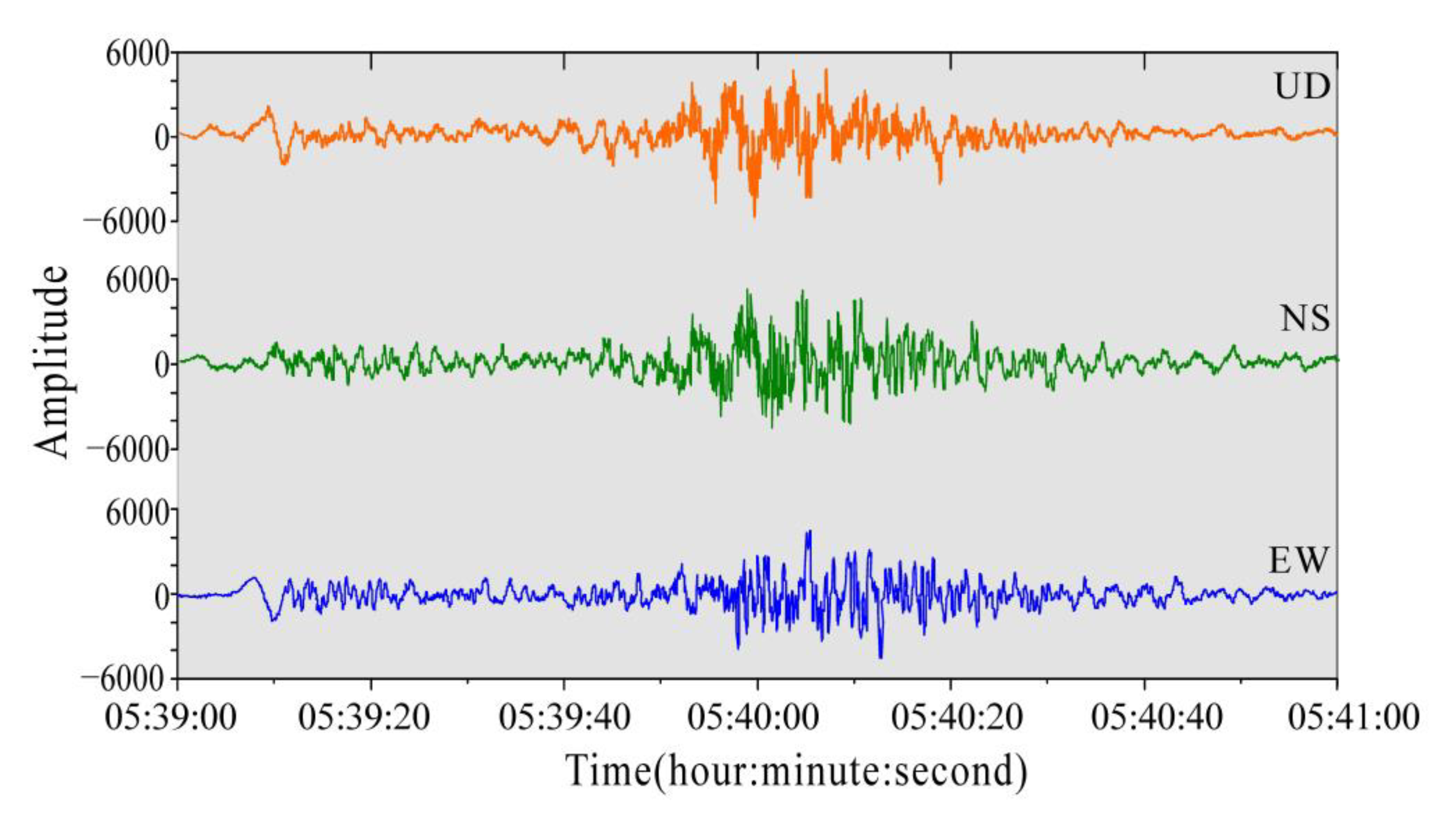
2.2. Seismic Signals

The National Seismic Network recorded the occurrence of an Ms 2.3 earthquake at 05:38:53 on 24 June 2017, in MaoXian County, Sichuan Province (N 32.08°, E 103.72°), with a focal depth of 0 km and no aftershocks reported. This earthquake was caused by the Xinmo landslide in MaoXian County. The seismic record of the landslide was completely recorded by the MaoXian Seismic Station (MXI), which was located about 47 km from the Xinmo landslide (Figure 1a). The entire shaking duration was about 121 s (Figure 2). Based on analysis of the seismic signal in the up-down (UD) direction, we investigated the characteristics of the landslide vibration signal recorded by the Maoxian Seismic Station (MXI). In addition, we studied the kinetic characteristics of the Xinmo landslide.

3. Methodology

3.1. Ensemble Empirical Mode Decomposition

The EEMD method is an empirical method proposed by Wu to deal with non-stationary time series and nonlinearly changing signals, and it is an improvement on the empirical mode decomposition (EMD) method [29]. The principle of the EMD method is to decompose the original signal based on the time scale characteristics of the signal and to obtain the sum of the intrinsic mode function (IMF) and the remainder (r) at different frequencies. Among them, the IMF represents the characteristics of the local information on different time scales. The remaining items are also called trend items, which represent the trend of the signal changes as follows [30]:

$$\mathrm{x}(t)={\displaystyle \sum _{\mathrm{i}=1}^N{f}_{imf}^i}+\gamma ,$$

(1)

where $\mathrm{x}(t)$ is the signal to be processed; $f_{imf}^i$ is the ith IMF (empirical mode decomposition function at each level); $\gamma$ is the trend item; and N is the total number of decomposed IMFs.

During the actual decomposition of the EMD signal, the signals of each eigenmode function are mixed, so the decomposed IMF cannot represent the local characteristics of the actual original signal. Therefore, Wu proposed the EEMD in 2009 to overcome this problem. In the EEMD method, white noise is introduced to construct a reference background for signal analysis, and then, the EMD method is used to decompose the signal, thus eliminating the mixing of the eigenmode signals. The specific steps are as follows [31]:

Step (1) Add a random Gaussian white noise signal to the original signal.

$${\mathrm{x}}_i(t)=\mathrm{x}\left(\mathrm{t}\right)+n{w}_i(t),$$

(2)

where ${\mathrm{x}}_i(t)$ is the processed signal; $\mathrm{x}\left(\mathrm{t}\right)$ is the signal to be processed; $w_i(t)$ is the added Gaussian white noise, i = 1, 2, 3……N; and $n$ is the amplitude coefficient.

Step (2) Decompose the items ${\mathrm{x}}_i(t)$ in step 1 sequentially using the EMD method to obtain m intrinsic mode decomposition functions (IMF) and one trend item.

$${\mathrm{x}}_i(t)={\displaystyle \sum _{j=1}^m{f}_{ij}^{}(t)}+{\gamma }_i(t),$$

(3)

where $f_{ij}^{}(t)$ is the jth eigenmode function obtained in the ith decomposition process. The other terms have the same meaning as above.

Step (3) Repeat steps 1 and 2 multiple times. It should be noted that the white noise added each time is added randomly and may not be the same.

Step (4) Average all of the obtained intrinsic mode functions (Equation (4)) to obtain the original signal decomposition results of the EEMD method.

$${\mathrm{x}}_i(t)=\frac{1}{N}({\displaystyle \sum _{i=}^N{\displaystyle \sum _{j=1}^m{f}_{ij}(t)}}+{\displaystyle \sum _{i=1}^N{\gamma }_i^{}(t)})$$

(4)

The EEMD method has been widely used in signal analysis research, especially for non-stationary and nonlinear signals, such as seismic signals, mechanical vibration signals, and photoelectric signals; however, few studies have been conducted on the decomposition of seismic signals generated by landslides. Wu suggested setting the number of white noise signals added N as 100 and the radiation coefficient as 0.2. At present, the research on the EEMD and EMD methods is relatively mature, and their related programs have also been packaged into a programming toolbox, which is convenience for decomposing landslide seismic signals [32].

3.2. Fourier Transformation

The landslide seismic signal can be transformed from the time-domain into the frequency-domain via Fourier transformation, and the signal characteristics such as the dominant frequency range and the amplitude of the signal frequency can be analyzed. This method has been widely used in the analysis of seismic signals, vibration signals, and sound waves. The basic formula is as follows [33]:

$$F(\omega )={\displaystyle \underset{-\infty }{\overset{+\infty }{\int }}\rho \left(\mathrm{t}\right)}\exp (-i\omega t)dt,$$

(5)

where $\omega$ is the signal frequency; $\mathrm{t}$ is the signal time; and $\exp (-i\omega t)$ is a complex variable function.

3.3. Time-Frequency Signal Analysis

The time-frequency analysis method mainly combines the time and frequency data to analyze the changes in the frequency with time [34]. Then, the signal can be divided according to the changes in the frequency amplitude. At present, there are many commonly used time-frequency signal analysis methods, such as the Winer-Ville method, short-time Fourier method, wavelet transformation method, and S transformation method. In this paper, the S change method is used [35,36,37]. This method uses a Gaussian window to analyze the relationship between the time signal and frequency [38]. As Equation (6) shows, it can effectively overcome the fluctuation caused by the signal instability and can better maintain the high resolution of the low frequency section. At present, this method has been compiled into a corresponding program, which can be implemented in the toolboxes of mainstream software programs such as Matlab and FORTRAN.

$$S(\tau ,f)={\displaystyle \underset{-\infty }{\overset{+\infty }{\int }}x(t)\frac{\left|f\right|}{\sqrt{2\pi }}}exp[-\frac{{(\tau -t)}^2{f}^2}{2}](-j2\pi ft)dt,$$

(6)

where f is the signal frequency; $\tau$ is the control parameter of the Gaussian window in time; t is time; j is an imaginary number; and $S(\tau ,f)$ is the S change result of the signal.

3.4. Numerical Analysis

Numerical simulation analysis is an important methods for analyzing the dynamic processes of landslides. The motion parameters obtained from the simulation mainly include the farthest motion distance, the maximum motion speed, and the thickness of the landslide deposits, which can be used to analyze the entire landslide process. In this paper, the particle discrete element method is used to conduct the simulation. This method mainly simulates the landslide body as a collection of particles and simulates the entire landslide movement process by analyzing the trajectories of the particles and the change in the force chain [39]. In addition, the interaction force between the particles is primarily determined based on contact theory. The contact model used in this paper is the Hertz-Mindlin (no slip) model, from which the equations of the tangential damping force, radial damping force, angular velocity, and angular acceleration between the particles can be obtained as follows [40,41]:

$$F_n^d=-2\sqrt{\frac{5}{6}}\beta \sqrt{S_n{m}^{\prime }}{v}_n^{rel},$$

(7)

$$F_t^d=-2\sqrt{\frac{5}{6}}\beta \sqrt{S_t{m}^{\prime }}{v}_t^{rel},$$

(8)

$$u_x(t_0)=\frac{F_x}{m},$$

(9)

$${\omega }_x(t_0)=\frac{M_x}{I_x},$$

(10)

where $F_{}^d$ is the damping force; $\beta$ is the contact coefficient; m′ is the equivalent mass; S is the stiffness; $v_{}^{rel}$ is the relative velocity; n denotes the normal direction; t denotes the tangential direction; $u_x$ is the average acceleration of the particle in the x direction at t₀; $F_x$ is the unbalanced force on the particle in the x direction; m is the mass of the particle; ${\omega }_x(t_0)$ is the average acceleration of the particle in the x direction at t₀; $M_x$ is the unbalanced moment on the particle in the x direction; and $I_x$ is the angular momentum of the particle in the x direction. The formulas for calculating the average acceleration and angular velocity of the particles in the y direction are similar to Equations (7) and (8) for the x direction, so they are not repeated here.

Based on a field geological survey and data collection, a 2-D discrete element numerical model of the Xinmo landslide was established. Considering the impact loading effect of the new landslide on the upper part of the old landslide, the particle-filled area was divided into the new landslide (red zone) and the old landslide accumulation area (Figure 3). The particle size in the new slide source area was 0.2–1 m, and the total number of particles was 1753. The particle size in the old landslide deposits was 0.2–0.8 m, and the total number of particles was 1685. The microscopic parameters of the particles, such as the density of the particles and slide bed, Poisson’s ratio, shear modulus, and other parameters, were mainly determined through numerical calibration tests (e.g., triaxial, direct shear, and angle of repose calibration tests) and from related research results [42,43,44]. For the contact parameters between the particles and the sliding bed, spherical particles were selected for use in the numerical tests. This is not consistent with the real situation, that is, the actual debris flow is mainly composed of rough irregularly shaped particles with edges and corners. According to the existing DEM contact parameter research results, we decided to appropriately reduce the rolling friction parameters of the particles and increase the static friction parameters between the sliding bed and the particles. The specific parameter values are presented in

Table 1. Particle and contact parameters used in discrete element simulation.

Parameter	Value
Particle/slide bed parameters
Density (kg/m3)	2600/2600 (particle/slide bed)
Poisson’s ratio	0.2/0.35 (particle/slide bed)
Shear deformation modulus (GPa)	21/7 (particle/slide bed)
Contact parameters
Coefficient of static friction between particles	0.5
Coefficient of rolling friction between particles	0.03
Particle recovery coefficient	0.5
Coefficient of static friction between particles and slide bed	0.8
Coefficient of rolling friction between particles and slide bed	0.05
Recovery coefficient of friction between particles and slide bed	0.35

.

4. Results and Analysis

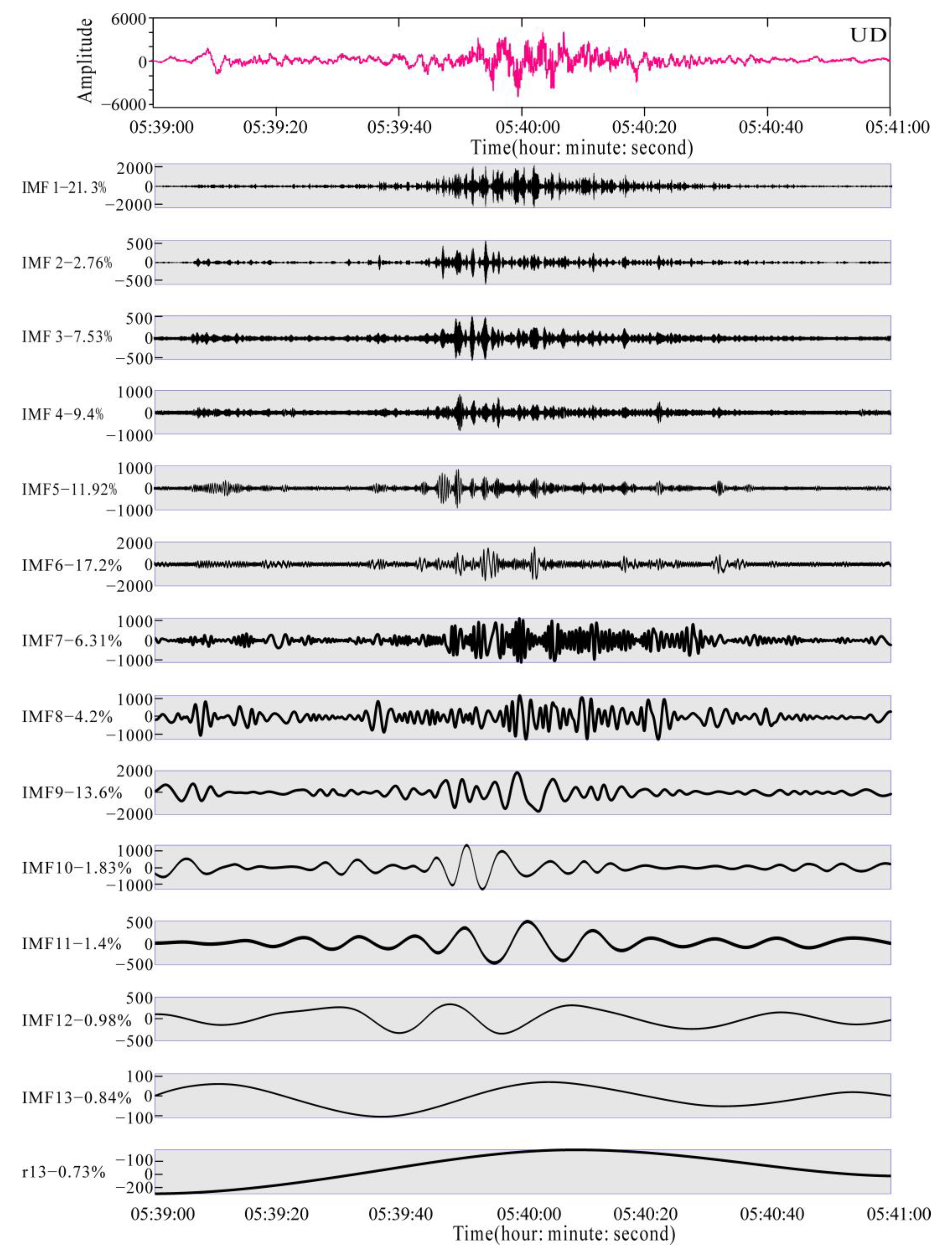
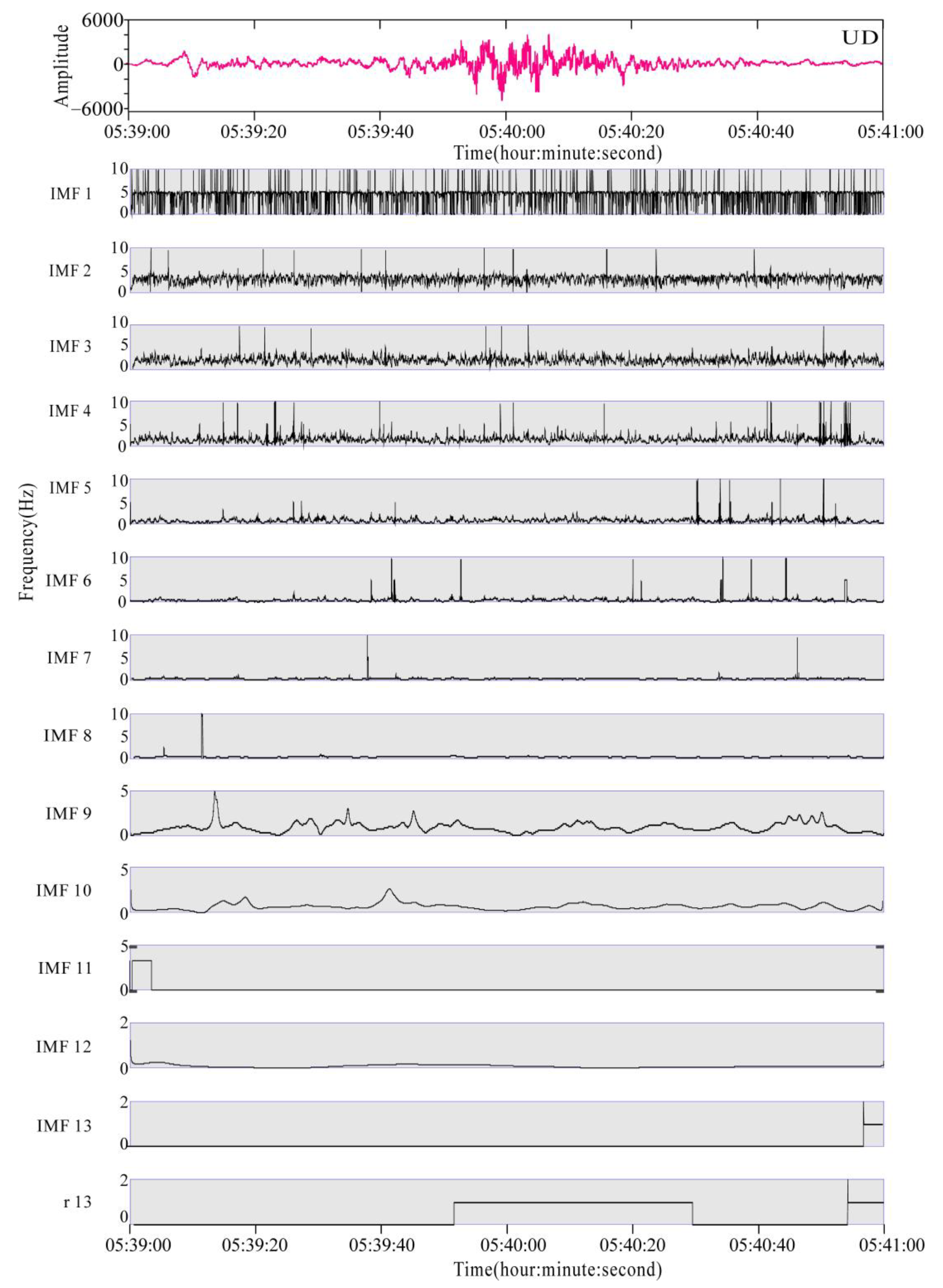
4.1. EEMD Characteristic Analysis

The seismic waveform produced by the Xinmo landslide and recorded by the Maoxian Seismic Station (MXI) is mainly composed of UD, north-south (NS) and east-west (EW) components, all of which can be used to characterize the movement process of the high-level Xinmo landslide. Due to several limitations, in this study, the UD vibration record was used to carry out the signal analysis. The vibration signal of the Xinmo landslide was decomposed into 13 modal eigenfunctions (IMF1–13) and one residual term (r) using the EEMD method. It can be seen from Figure 4 that the energy proportions of IMF1–13 are 21.3%, 7.53%, 9.4%, 11.92%, 17.2%, 6.31%, 4.2%, 13.6%, 1.83%, 1.4%, 0.98%, and 0.84%, respectively. Based on the time history curves of each IMF, IMF-5 characterizes the fluctuation characteristics of the original landslide signal better, and IMF-5 exhibits obvious vibrations in the two intervals from 39 m at 5.0 s to 39 m at 18.9 s and from 39 m at 38.0 s to 40 m at 36 s. According to the field geological survey and impact force analysis, the first interval represents the continuous loading after the rapid initiation of the landslide, and the latter interval represents the overall instability stage of the landslide after the impact loading and until the old landslide became unstable. The IMFs were analyzed from the perspective of the instantaneous frequency (Figure 5), the frequency range of IMF1–8 was 0–10 Hz, the frequency range of IMF9–11 was 0–5 Hz, and the frequency range of IMF12–13 was 0–2 Hz.

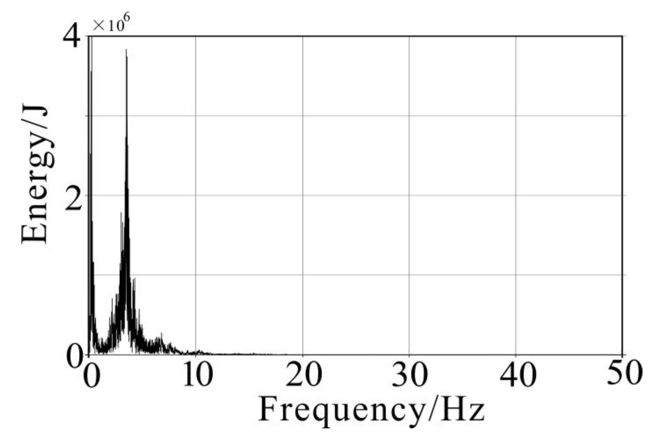
4.2. Spectral Analysis and Time History Analysis

The Fourier transform analysis of the UD component of the Xinmo landslide vibration signal revealed that the vibration signal was dominated by low frequencies of 0–10 Hz, and the energy was mainly concentrated within 2–8 Hz (Figure 6), which corresponded to the typical characteristic frequencies of the IMFs obtained via EEMD decomposition. Therefore, it was quickly determined to be a landslide-induced earthquake based on the frequency composition characteristics of the seismic signal. This provided a basis for the next step of the analysis of the evolution of the sliding motion.

According to the frequency range and amplitude change characteristics of the time-frequency signal, the motion was divided into four stages (

Table 2. Division of landslide movement stages based on time-frequency diagram.

Order	Stage	Start Time	Stop Time	Duration (s)	Distance (m)	Average Speed (m/s)	Main Frequency Range (Hz)
a	Rapid start	05:39:00	05:39:29	29/120	380	13.1	2.6–4.6
b	Impact loading	05:39:29	05:39:47	18/120	350	19.4	3.2–5.7
c	Fragmentation and migration	05:39:47	05:40:26	39/120	1150	29.4	2.8–8.5
d	Scattered accumulation	05:40:26	05:41:00	34/120	850	25.0	2.1–5.2

, Figure 7): rapid start, impact loading, fragmentation and migration, and scattered accumulations stages.

The first stage was the rapid start stage (Figure 7a). This stage started at 05:39:00, ended at 05:39:29, and lasted for about 29 s. The landslide initiated rapidly due to the occurrence of collapse. The slope length of the slide source area was about 380 m, and the average speed of the movement of the material from the trailing edge of the landslide to the shear outlet was about 13.1 m/s. The main frequency range of this stage was 2.6–4.6 Hz.

The second stage was the impact loading stage (Figure 7b). This stage started at 05:39:29, ended at 05:39:47, and lasted for about 18 s. In this stage, an ~350 × 10⁴ m³ sliding mass was loaded to the middle and back sections of the old landslide mass, which caused the the old landslide mass to become unstable. Since the length of the covering area was about 350 m, the average velocity of the sliding body was about 19.4 m/s. Compared with the rapid start stage, the energy and frequency of this stage were significantly higher. The main frequency range of this stage was 3.2–5.7 Hz.

The third stage was the fragmentation and migration stage (Figure 7c). This stage started at 05:39:47, ended at 05:40:26, and lasted for about 39 s. In this stage, under the action of the impact load, the sliding body was severely broken, and the old landslide body was destabilized and reactivated, causing the sliding body to exhibit debris flow type movement. This stage was the main sliding movement stage. The energy and frequency were still high, and the main frequency range was 2.8–8.5 Hz. The movement distance of the sliding body reached 1150 m, and the average movement speed was about 29.4 m/s.

The fourth stage was the scattered accumulation stage (Figure 7d). This stage started at 05:40:26, ended at 05:41:00 s, and lasted for about 34 s. As the terrain became more open, the slippery bodies scattered and accumulated in the surrounding area, and the movement gradually slowed down. In this stage, the energy and frequency began to decrease compared with the previous three stages, and the dominant frequency range was 2.1–5.2 Hz. The movement distance of the sliding body was about 850 m, and the average movement speed was about 25.0 m/s.

In summary, the total duration of the Xinmo landslide’s movement was about 120 s, the movement distance was about 2750 m, and the average movement speed was about 22.9 m/s, making this a typical high-level long-distance landslide disaster.

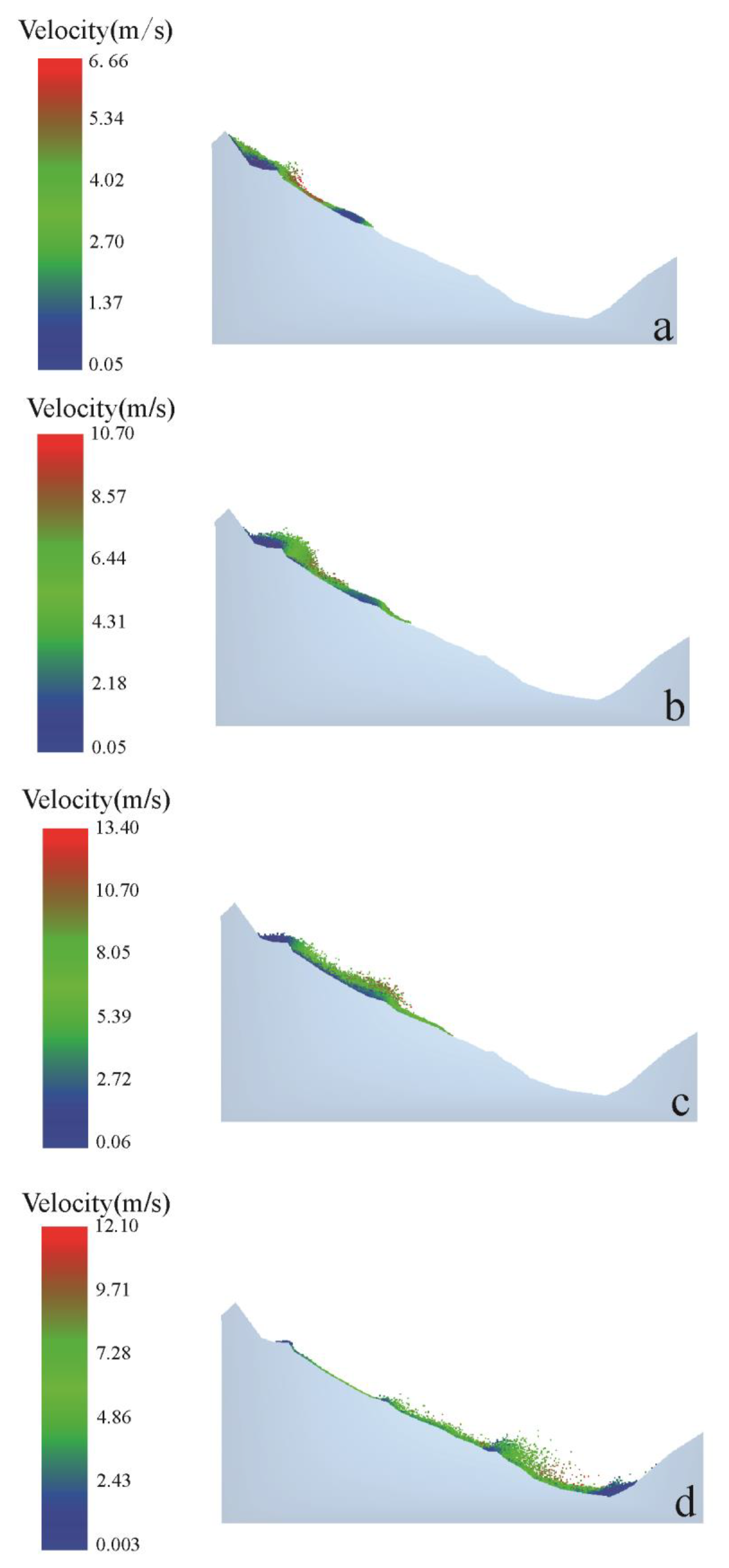
4.3. Analysis of Numerical Simulation Results

The numerical simulation results show that the total duration of the landslide movement was about 120 s, the farthest movement distance was about 2830 m, and the average speed was 23.58 m/s, which are similar to the seismic analysis results. At a horizontal distance of about 1175 m, the velocity reached a maximum velocity of 62.3 m/s (Figure 8). The specific movement process was as follows. After the sliding mass rapidly began to slide, some of the particles at the front edge moved to the middle and rear of the old landslide body, and the velocity at the front edge was about 6.66 m/s (Figure 9a). The movement speed of the particles on the surface of the slip source area was fast, about 1.37–4.02 m/s. The particles inside the slip source area were still in a relatively static state. When the landslide mass slid on a large scale, continuous impact loading was applied to the middle and back sections of the old landslide body, and the surface particles on the old landslide were scraped and entrained. The front edge reached a maximum velocity of 10.7 m/s (Figure 9b). According to the particle counter statistics, about 424 particles, that is, 0.17 × 10⁴ m³ particles, hit the front edge of the old landslide and slipped at a speed of about 3 m/s. When about 722 particles had accumulated, that is, 0.29 × 10⁴ m³ particles were loaded on the old landslide body, the old landslide lost its stability and slid as a whole (Figure 9c). The numerical model established in this study was a two-dimensional model. When the result of the 2-D model was converted into a three-dimensional model, the loading volume that led to the instability of the ancient landslide was (0.29 × 10⁴) × 350 = 101 × 10⁴ m³, where 350 m was the width of the landslide source area. At this time, the average speed of the sliding body was about 8.05 m/s. When the sliding body impacted on the old landslide, it destabilized and reactivated the old landslide. In addition, the landslide scraped and entrained the loose deposits of the old landslide, and then, it transformed into a landslide debris flow, exhibiting overall sliding (Figure 9d). Finally, the leading edge of the landslide was blocked by the opposite mountain, and it began to gradually stagnate. The average accumulation thickness of the accumulation body reached 30 m, and there was no accumulation in the slip source area and the debris flow area. This was mainly because the particles were greatly affected by the slope of the terrain and could not be fixed on the slope.

5. Discussion

In traditional landslide geological hazard divisions, the landslide is generally divided into a landslide source area, debris flow area, and accumulation area [45,46,47,48]. This classification method is primarily based on the spatial-temporal characteristics of each region [49]. This classification method helps us understand the mechanism of landslide movement in the early stage, but it ignores the characteristics of high-level landslides such as strong impact loading and a hidden disaster-forming process. According to the results of the field geological survey and the seismic signal analysis, in this paper, we propose a new division method for high-level landslide hazards (Figure 10), including four zones: rapid star, impact loading, fragmentation and migration, and scattered accumulation zones (Figure 10).

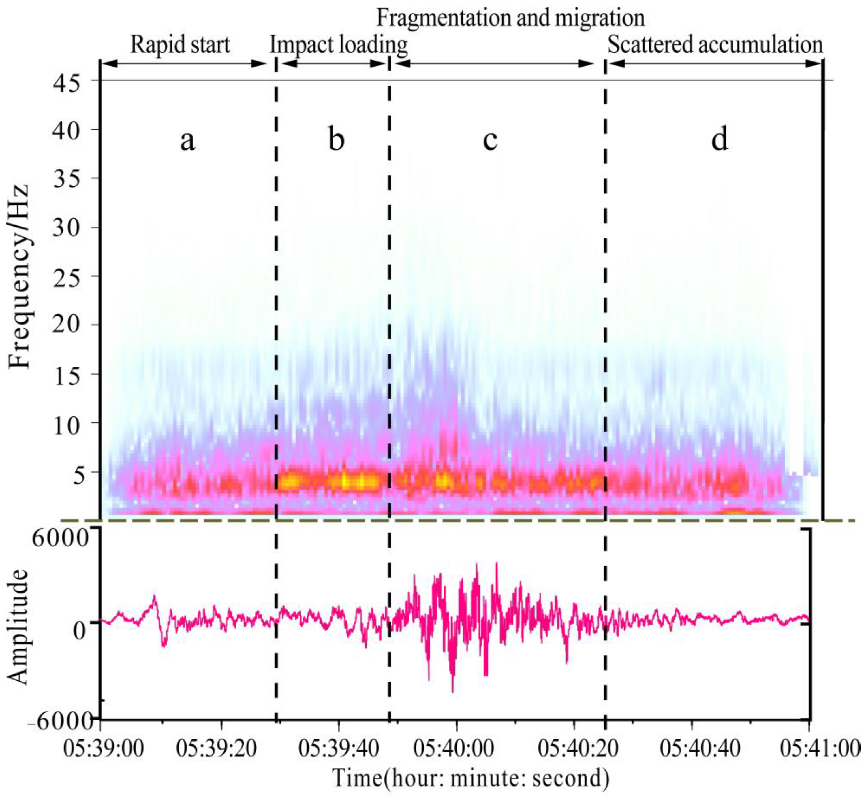
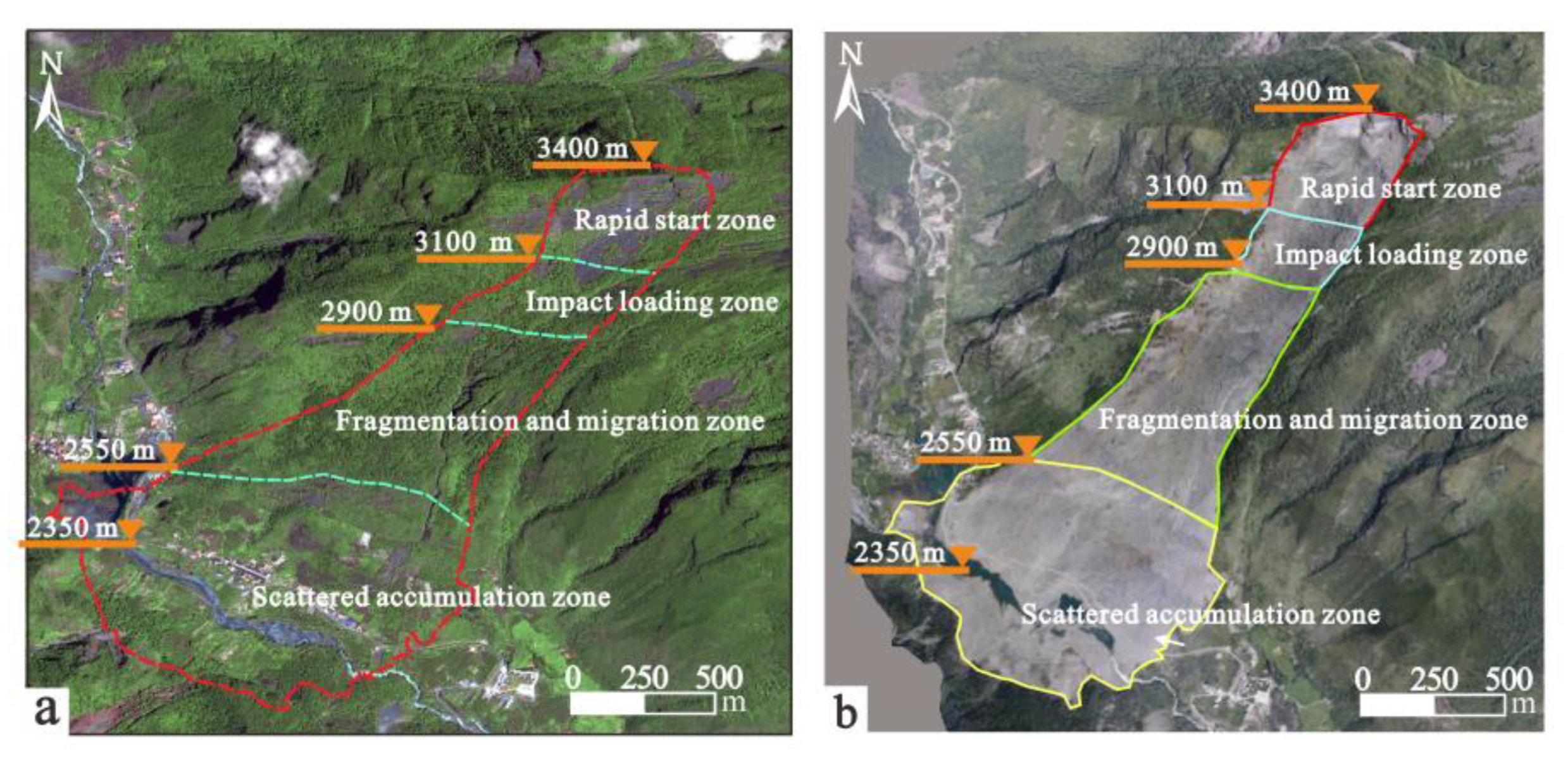
(1)

Rapid start zone

In the high-level landslide rapid start zone (elevations of 3100–3400 m), the sliding force of the landslide body gradually increased under the action of the earthquake, rainfall, and freezing-thawing. Thus, the internal energy of the locked section of the rock mass gradually increased, and the locked section finally ruptured [50]. At the moment when the sliding body was cut out, the energy released increased the kinetic energy of the landslide, resulting in the sliding body having a higher initial velocity at the beginning of its movement process.

(2)

Impact loading zone

In the impact loading area (elevations of about 2900–3100 m), because the surface was covered with loose deposits created by the 1933 earthquake, it was defined as the old landslide mass. Before the occurrence of the Xinmo landslide, due to the weathering and erosion of the parent rock in the rapid start zone, the loose stones on the surface of the parent rock fell off, and they were scattered and accumulated in the impact loading area, creating inverted stone cones and defining the initial scope of the impact loading area. After the large-scale shearing of the sliding body in the rapid start zone, the sliding body was continuously loaded to the middle and rear of the old landslide body, and the strong kinetic impact force caused instability and sliding. The numerical simulation results indicate that when the 101 × 10⁴ m³ sliding mass was loaded on the old landslide accumulation, the old landslide mass became unstable and was reactivated.

(3)

Fragmentation and migration zone

In the fragmentation migration area (elevations of about 2550–2900 m), due to the dynamic impact loading force, the sliding bodies collided with each other, broke, and disintegrated; and the number of block fractals gradually increased. Moreover, limited by the terrain, the movement path of the Xinmo landslide was pipe-shaped. During the movement of the sliding body, it proceeded in the movement mode of a continuous debris flow. It scraped the loose accumulation on the ground, further increasing the volume of the sliding body.

(4)

Scattered accumulation zone

In the scattered accumulation area (elevations of about 2350–2550 m), due to the gentle slope, the sliding mass transformed from a pipe-shaped mass into a diffuse debris flow, resulting in a fan-shaped accumulation. During the movement and accumulation process, the sliding bodies squeezed or sheared each other, forming a motion ridge landform. The accumulation body was divided into block stone facies, slide body facies, and bedrock facies from top to bottom, and some of the block stones were cracked but not scattered, forming a puzzle structure. Finally, the sliding body was blocked by the terraces and mountains on the other side, and its movement speed gradually decreased until the accumulation stopped.

In summary, compared with the traditional landslide hazard zonation method, the hazard zonation method proposed in this paper highlights the kinetic characteristics of high-level landslides (Figure 10). Most high-level landslides are caused by the rupture of a locked section, which releases the energy of the sliding mass, leading to the sliding mass having a high initial velocity. High-level landslides generally have a large volume (>100 × 10⁴ m³). The huge landslide hits the loose accumulation on the ground surface, causing it to become destabilized and to reactivate, and thus, the volume of the landslide increases [51]. When the Yigong landslide occurred in Tibet in 2000, an ~3 × 10⁷ m³ landslide mass impacted the loose deposits formed by the 1990 landslide in the ditch. The resulting strong compaction effect resulted in the sliding mass colliding with and engulfing the old landslide accumulation, and the final accumulation volume reached 3 × 10⁸ m³ [52]. Tectonic movements are active in alpine and canyon areas, and old landslides are widely distributed. Current research has mainly focused on the stability of ancient landslides under rainfall, earthquakes, and human engineering activities and has largely ignored the impact of high-level kinetic impact loading on destabilization and revival of ancient landslides [53,54]. After the impact loading stage, the sliding mass broke up and disintegrated, exhibiting debris flow type migration, and finally, the accumulation stopped after being blocked by mountains and rivers, forming long-distance accumulation landforms such as motion ridges [55,56]. The zonation of high-level landslide hazards improves our understanding the evolution stages of the dynamic process of such landslides, strengthens our understanding of landslide kinetic mechanisms, and provides important guidance for high-level landslide risk assessment and other work.

In view of the analysis and research on the dynamic process of a high-position and long runout landslide in western China, scholars have carried out some effective numerical analyses and research on the dynamic process [57,58,59,60]. The numerical simulation methods used included the empirical method, continuum method, and discrete element method. Among them, the empirical method has relatively simple calculations and is mostly used in the emergency rescue stage. It is relatively conservative in evaluating the landslide speed, and it is feasible to use it in risk planning. Considering the changes in the topography and geomorphology, the continuum method can simulate a high-level landslide under complex terrain conditions, and it provides a variety of base resistance models, but it cannot show the interaction force such as the collision between the blocks inside the sliding body. The discrete element method can better simulate the collision and accumulation characteristics of sliding bodies and can completely show the dynamic processes such as the rapid start, impact loading, and reactivation of the old landslide. The above method provides technical support for studying the dynamic disaster effect of high landslides.

6. Conclusions

Due to its huge destructiveness, the study of the kinetic disaster effect of the high-level Xinmo landslide has been the focus of research. Based on a large amount of previous research, in this study, the movement process of the Xinmo landslide was investigated via landslide seismic signal analysis and discrete element numerical simulation. The main conclusions of this study are as follows.

(1)

In the seismic signal analysis, the Xinmo landslide vibration signal was decomposed into 13 modal eigenfunctions and one remainder via ensemble empirical mode analysis, and the energy proportion of each modal eigenfunction was calculated. Through spectrum analysis, it was found that the frequency of the landslide vibration signal was mainly low, the vibration signal was mainly located at low frequencies of 0–10 Hz, and the dominant frequency range was 2–8 Hz. This provides a method for the preliminary identification of landslide seismic signals.

(2)

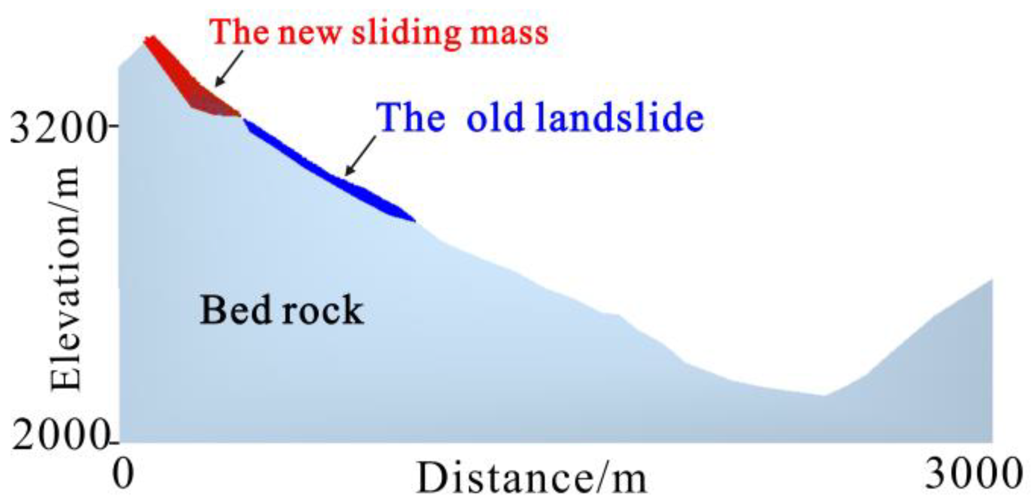
According to the discrete element calculation results, when the 101 × 10⁴ m³ sliding mass was loaded on the old landslide accumulation, the old landslide mass became unstable and was reactivated. At a horizontal distance of 1175 m, the maximum speed of the sliding body was 69.93 m/s. By comparing the continuum method and the sled model, it was determined that the discrete element method can better describe the kinetic impact behavior of high-level landslides.

(3)

Regarding high-level landslide kinetic disaster zoning, in this study, seismic signal analysis and discrete element calculation analysis were combined and the traditional zoning method based on the spatial relationships of the landslide sections was replaced with a new zoning method based on the kinetic behavior of the landslide. The proposed landslide division includes rapid start, impact loading, fragmentation and migration, and scattered accumulation zones. We also preliminarily analyzed the kinetic characteristics and geomorphic characteristics of each region. The results of this study have important guiding significance for risk assessment of high-level landslides. And these also provide a basis for the formulation of land use planning in mountainous areas, and promote economic construction and sustainable development in mountainous areas.

References

- Yin, Y.; Li, B.; Gao, Y.; Wang, W.; Zhang, S.; Zhang, N. Geostructures, dynamics and risk mitigation of high-altitude and long-runout rockslides. J. Rock Mech. Geotech. Eng. 2023, 15, 66–101. [Google Scholar] [CrossRef]
- Liu, S.; Wang, L.; Zhang, W.; He, Y.; Pijush, S. A comprehensive review of machine learning-based methods in landslide susceptibility mapping. Geol. J. 2023, 1–19. [Google Scholar] [CrossRef]
- Hungr, O.; Leroueil, S.; Picarelli, L. The Varnes classification of landslide types, an update. Landslides 2013, 11, 167–194. [Google Scholar] [CrossRef]
- Fan, X.; Yunus, A.P.; Scaringi, G.; Catani, F.; Subramanian, S.S.; Xu, Q.; Huang, R. Rapidly evolving controls of landslides after a strong earthquake and implications for hazard assessments. Geophys. Res. Lett. 2020, 1, 48. [Google Scholar] [CrossRef]
- Allstadt, K. Extracting source characteristics and dynamics of the August 2010 Mount Meager landslide from broadband seismograms. J. Geophys. Res. Earth Surf. 2013, 118, 1472–1490. [Google Scholar] [CrossRef]
- Ekstrom, G.; Stark, C.P. Simple Scaling of Catastrophic Landslide Dynamics. Science 2013, 339, 1416–1419. [Google Scholar] [CrossRef] [Green Version]
- Zhang, Z.; He, S. Analysis of broadband seismic recordings of landslide using empirical Green’s function. Geophys. Res. Lett. 2019, 46, 4628–4635. [Google Scholar] [CrossRef]
- Fan, X.; Xu, Q.; Alonso-Rodriguez, A.; Subramanian, S.S.; Li, W.; Zheng, G.; Dong, X.; Huang, R. Successive landsliding and damming of the Jinsha River in eastern Tibet, China: Prime investigation, early warning, and emergency response. Landslides 2019, 16, 1003–1020. [Google Scholar] [CrossRef]
- Zhuang, Y.; Xing, A.; Leng, Y.; Bilal, M.; Zhang, Y.; Jin, K.; He, J. Investigation of Characteristics of Long Runout Landslides Based on the Multi-Source Data Collaboration: A Case Study of the Shuicheng Basalt Landslide in Guizhou, China. Rock Mech. Rock Eng. 2021, 54, 3783–3798. [Google Scholar] [CrossRef]
- Zhang, C.; Yin, Y.; Yan, H.; Zhu, S.; Li, B.; Hou, X.; Yang, Y. Centrifuge modeling of multi-row stabilizing piles reinforced reservoir landslide with different row spacings. Landslides 2022, 20, 559–577. [Google Scholar] [CrossRef]
- Suriñach, E.; Vilajosana, I.; Khazaradze, G.; Biescas, B.; Furdada, G.; Vilaplana, J.M. Seismic detection and characterization of landslides and other mass movements. Nat. Hazards Earth Syst. Sci. 2005, 5, 791–798. [Google Scholar] [CrossRef] [Green Version]
- Yamada, M.; Kumagai, H.; Matsushi, Y.; Matsuzawa, T. Dynamic landslide processes revealed by broadband seismic records. Geophys. Res. Lett. 2013, 40, 2998–3002. [Google Scholar] [CrossRef]
- Helmstetter, A.; Garambois, S. Seismic monitoring of Sechilienne rockslide (FrenchAlps): Analysis of seismic signals and their correlation with rainfalls. J. Geophys. Res.-Earth Surf. 2010, 115, 03016. [Google Scholar] [CrossRef]
- Yan, Y.; Cui, Y.; Tian, X.; Hu, S.; Guo, J.; Wang, Z.; Yin, S.; Liao, L. Seismic signal recognition and interpretation of the (2019) 7.23. Shuicheng Landslide by Seismogram Stations. Landslides 2020, 17, 1191–1206. [Google Scholar] [CrossRef]
- Dammeier, F.; Moore, J.R.; Haslinger, F.; Loew, S. Automatic detection of alpine rockslides in continuous seismic data using hidden Markov models. J. Geophys. Res.-Earth Surf. 2016, 121, 351–371. [Google Scholar] [CrossRef] [Green Version]
- Li, Z.-Y.; Huang, X.-H.; Yu, D.; Su, J.-R.; Xu, Q. Broadband-seismic analysis of a massive landslide in southwestern China: Dynamics and fragmentation implications. Geomorphology 2019, 336, 31–39. [Google Scholar] [CrossRef]
- An, H.; Ouyang, C.; Zhou, S. Dynamic process analysis of the Baige landslide by the combination of DEM and long-period seismic waves. Landslides 2021, 18, 1625–1639. [Google Scholar] [CrossRef]
- Wang, L.Q.; Xiao, T.; Liu, S.L.; Zhang, W.G.; Yang, B.B.; Chen, L.C. Quantification of model uncertainty and variability for landslide displacement prediction based on Monte Carlo simulation. Gondwana Res. 2023, 1–43. [Google Scholar] [CrossRef]
- Mancarella, D.; Hungr, O. Analysis of run-up of granular avalanches against steep, adverse slopes and protective barriers. Can. Geotech. J. 2010, 47, 827–841. [Google Scholar] [CrossRef]
- Liu, G.; Ma, F.; Zhang, M.; Guo, J.; Jia, J. Y-Mat: An improved hybrid finite-discrete element code for addressing geotechnical and geological engineering problems. Eng. Comput. 2022, 39, 1962–1983. [Google Scholar] [CrossRef]
- Carrión-Mero, P.; Montalván-Burbano, N.; Morante-Carballo, F.; Quesada-Román, A.; Apolo-Masache, B. Worldwide Research Trends in Landslide Science. Int. J. Environ. Res. Public Health 2021, 18, 9445. [Google Scholar] [CrossRef] [PubMed]
- Yin, Y.; Wang, W.; Zhang, N.; Yan, J.; Wei, Y. The June 2017 Maoxian landslide: Geological disaster in an earthquake area after the Wenchuan Ms 8.0 earthquake. Sci. China Technol. Sci. 2017, 60, 1762–1766. [Google Scholar] [CrossRef]
- Fan, X.; Xu, Q.; Scaringi, G.; Dai, L.; Li, W.; Dong, X.; Zhu, X.; Pei, X.; Dai, K.; Havenith, H.-B. Failure mechanism and kinematics of the deadly June 24 2017 Xinmo landslide, Maoxian, Sichuan, China. Landslides 2017, 14, 2129–2146. [Google Scholar] [CrossRef]
- Scaringi, G.; Fan, X.; Xu, Q.; Liu, C.; Ouyang, C.; Domènech, G.; Yang, F.; Dai, L. Some considerations on the use of numerical methods to simulate past landslides and possible new failures: The case of the recent Xinmo landslide (Sichuan, China). Landslides 2018, 15, 1359–1375. [Google Scholar] [CrossRef]
- Wang, Y.; Zhao, B.; Li, J. Mechanism of the catastrophic June 2017 landslide at Xinmo Village, Songping River, Sichuan province, china. Landslides 2017, 15, 333–345. [Google Scholar] [CrossRef]
- Wang, W.; Yin, Y.; Yang, L.; Zhang, N.; Wei, Y. Investigation and dynamic analysis of the catastrophic rockslide avalanche at Xinmo, Maoxian, after the Wenchuan Ms 8.0 earthquake. Bull. Eng. Geol. Environ. 2019, 79, 495–512. [Google Scholar] [CrossRef]
- Meng, W.; Xu, Y.; Cheng, W.C.; Arulrajah, A. Landslide hazards on June 24 in Sichuan province, China: Preliminary investigation and analysis. Geosciences 2018, 8, 39. [Google Scholar] [CrossRef] [Green Version]
- Yang, L.; Wang, W.; Zhang, N.; Wei, Y. Characteristics and numerical runout modeling analysis of the Xinmo landslide in Sichuan, China. Earth Sci. Res. J. 2020, 24, 167–179. [Google Scholar] [CrossRef]
- Wu, Z.; Huang, N.E. Ensemble empirical mode decomposition: A noise-assisted data analysis method. Adv. Adapt. Data Anal. 2009, 1, 1–41. [Google Scholar] [CrossRef]
- Huang, N.E.; Wu, C.M.-L.; Long, S.R.; Shen, S.S.P.; Ou, W.; Gloersen, P.; Fan, K.L. A confidence limit for the empirical mode decomposition and Hilbert spectral analysis. Proc. R. Soc. Lond. Ser. A Math. Phys. Eng. Sci. 2003, 459, 2317–2345. [Google Scholar] [CrossRef]
- Wang, W.-C.; Chau, K.-W.; Xu, D.-M.; Chen, X.-Y. Improving Forecasting Accuracy of Annual Runoff Time Series Using ARIMA Based on EEMD Decomposition. Water Resour. Manag. 2015, 29, 2655–2675. [Google Scholar] [CrossRef]
- Wang, S.; Zhang, N.; Wu, L.; Wang, Y. Wind speed forecasting based on the hybrid ensemble empirical mode decomposition and GA-BP neural network method. Renew. Energy 2016, 94, 629–636. [Google Scholar] [CrossRef]
- Auslander, L.; Grunbaum, F.A. The Fourier transform and the discrete Fourier transform. Inverse Probl. 1989, 5, 149. [Google Scholar] [CrossRef]
- Cohen, L. Time–frequency distributions: A review. Proc. IEEE 1989, 7, 941–981. [Google Scholar] [CrossRef] [Green Version]
- Fonollosa, J.R.; Nikias, C.L. Wigner higher-order moment spectra: Definitions, properties, computation and application to transient signaldetection. IEEE Trans. SP 1993, 7, 842–853. [Google Scholar] [CrossRef]
- Mallat, S. A theory for multi-resolution signal representation: The wavelet transform. IEEE Trans. PAM I 1989, 11, 674–693. [Google Scholar] [CrossRef] [Green Version]
- Marple, L. A new autoregressive spectrum analysis algorithm. IEEE Trans. ASSP 1990, 8, 441–450. [Google Scholar] [CrossRef]
- Assous, S.; Boashash, B. Evaluation of the modified S-transform for time-frequency synchrony analysis and source localization. EURASIP J. Adv. Signal Process. 2012, 49, 1–18. [Google Scholar]
- Cundall, P.A.; Strack, O.D.L. A discrete numerical model for granular assemblies. Geotechnique 1979, 29, 47–65. [Google Scholar] [CrossRef]
- Wang, W.; Yin, Y.; Zhu, S.; Wang, L.; Zhang, N.; Zhao, R. Investigation and numerical modeling of the overloading-induced catastrophic rockslide avalanche in Baige, Tibet, China. Bull. Eng. Geol. Environ. 2020, 79, 1765–1779. [Google Scholar] [CrossRef]
- EDEM 2.4. Theory Reference Guide; DEM Solutions: Edinburgh, UK, 2011.
- Luo, H.; Xing, A.; Jin, K.; Xu, S.; Zhuang, Y. Discrete Element Modeling of the Nayong Rock Avalanche, Guizhou, China Constrained by Dynamic Parameters from Seismic Signal Inversion. Rock Mech. Rock Eng. 2021, 54, 1629–1645. [Google Scholar] [CrossRef]
- Wang, W.; Yin, Y.; Wei, Y.; Zhu, S.; Li, J.; Meng, H.; Zhao, R. Investigation and characteristic analysis of a high-position rockslide avalanche in Fangshan District, Beijing, China. Bull. Eng. Geol. Environ. 2021, 80, 2069–2084. [Google Scholar] [CrossRef]
- Zhang, S.-L.; Yin, Y.-P.; Hu, X.-W.; Wang, W.-P.; Zhang, N.; Zhu, S.-N.; Wang, L.-Q. Dynamics and emplacement mechanisms of the successive Baige landslides on the Upper Reaches of the Jinsha River China. Eng. Geol. 2020, 278, 105819. [Google Scholar] [CrossRef]
- Mitchell, A.; McDougall, S.; Aaron, J.; Brideau, M.-A. Rock Avalanche-Generated Sediment Mass Flows: Definitions and Hazard. Front. Earth Sci. 2020, 8, 543937. [Google Scholar] [CrossRef]
- Knapp, S.; Krautblatter, M. Conceptual Framework of Energy Dissipation During Disintegration in Rock Avalanches. Front. Earth Sci. 2020, 8, 263. [Google Scholar] [CrossRef]
- Guo, Z.; Chen, L.; Yin, K.; Shrestha, D.P.; Zhang, L. Quantitative risk assessment of slow-moving landslides from the viewpoint of decision-making: A case study of the Three Gorges Reservoir in China. Eng. Geol. 2020, 273, 105667. [Google Scholar] [CrossRef]
- Guo, Z.; Ferrer, J.V.; Hürlimann, M.; Medina, V.; Puig-Polo, C.; Yin, K.; Huang, D. Shallow landslide susceptibility assessment under future climate and land cover changes: A case study from southwest China. Geosci. Front. 2023, 14, 101542. [Google Scholar] [CrossRef]
- Zhang, T.; Yin, Y.; Li, B.; Liu, X.; Wang, M.; Gao, Y.; Wan, J.; Gnyawali, K.R. Characteristics and dynamic analysis of the February 2021 long-runout disaster chain triggered by massive rock and ice avalanche at Chamoli, Indian Himalaya. J. Rock Mech. Geotech. Eng. 2023, 15, 296–308. [Google Scholar] [CrossRef]
- Medina, V.; Hürlimann, M.; Guo, Z.; Lloret, A.; Vaunat, J. Fast physically-based model for rainfall-induced landslide susceptibility assessment at regional scale. Catena 2021, 201, 105213. [Google Scholar] [CrossRef]
- Shao, C.; Li, Y.; Lan, H.; Li, P.; Zhou, R.; Ding, H.; Yan, Z.; Dong, S.; Yan, L.; Deng, T. The role of active faults and sliding mechanism analysis of the 2017 Maoxian postseismic landslide in Sichuan, China. Bull. Eng. Geol. Environ. 2019, 78, 5635–5651. [Google Scholar] [CrossRef]
- Hungr, O.; Evans, S.G. Entrainment of debris in rock avalanches: An analysis of a long run-out mechanism. Geol. Soc. Am. Bull. 2004, 116, 1240–1252. [Google Scholar] [CrossRef] [Green Version]
- Huang, R.Q. Large-scale Landslides and Their Sliding Mechanisms in China Since the 20th Century. China J. Rock Mech. Eng. 2007, 26, 433–454. [Google Scholar]
- Dai, F.; Lee, C.; Deng, J.; Tham, L. The 1786 earthquake-triggered landslide dam and subsequent dam-break flood on the Dadu River, southwestern China. Geomorphology 2005, 73, 277–278. [Google Scholar] [CrossRef]
- Barla, G.; Debernardi, D.; Perino, A. Lessons learned from deep-seated landslides activated by tunnel excavation. Geomech. Tunn. 2015, 8, 394–401. [Google Scholar] [CrossRef]
- Weidinger, J.T.; Korup, O.; Munack, H.; Altenberger, U.; Dunning, S.A.; Tippelt, G.; Lottermoser, W. Giant rockslides from the inside. Earth Planet. Sci. Lett. 2014, 389, 62–73. [Google Scholar] [CrossRef]
- Wang, Y.-F.; Cheng, Q.-G.; Lin, Q.-W.; Li, K.; Yang, H.-F. Insights into the kinematics and dynamics of the Luanshibao rock avalanche (Tibetan Plateau, China) based on its complex surface landforms. Geomorphology 2018, 317, 170–183. [Google Scholar] [CrossRef]
- Chang, W.; Xu, Q.; Dong, X.; Zhuang, Y.; Xing, A.; Wang, Q.; Kong, X. Dynamic process analysis of the Xinmo landslide via seismic signal and numerical simulation. Landslides 2022, 19, 1463–1478. [Google Scholar] [CrossRef]
- Jin, K.; Xing, A.; Chang, W.; He, J.; Gao, G.; Bilal, M.; Zhang, Y.; Zhuang, Y. Inferring Dynamic Fragmentation Through the Particle Size and Shape Distribution of a Rock Avalanche. J. Geophys. Res. Earth Surf. 2022, 127, e2022JF006784. [Google Scholar] [CrossRef]
- Yang, L.; Wei, Y.; Wang, W.; Zhu, S. Numerical Runout Modeling Analysis of the Loess Landslide at Yining, Xinjiang, China. Water 2019, 11, 1324. [Google Scholar] [CrossRef] [Green Version]