A Time-and-Space-Network-Based Green Fleet Planning Model and Its Application for a Hub-and-Spoke Network

Abstract

Most previous studies on airline fleet planning have focused solely on economic considerations, neglecting the impact of carbon reduction. This paper presents a novel method for green fleet planning, using a bi-level programming model to balance conflicts among stakeholders while considering uncertain parameters such as demand and operating costs. The upper model aims to reduce carbon emissions by taking into account government constraints, such as carbon allowances and carbon prices, as well as airline satisfaction. The lower model seeks to maximize airline revenue using a space-and-time network model based on given airline flight schedules. To verify the game model, a case study utilizing randomly generated scenarios is employed within the context of China’s aviation-specific emissions trading scheme. Results show that: (1) compared to the scenario without a policy aiming at reducing carbon emissions, this method reduces carbon emissions by 23.03% at the expense of a 6.96% reduction in terms of the airline’s operating profit; (2) when passenger demand levels increase to 160%, the profitability of the proposed fleet increases by 50.83%, while there were only insignificant changes in carbon emissions; (3) the proposed methodology can assist the airlines systematically to reduce carbon emissions and provide valuable strategic guidance for policy makers.

1. Introduction

Carbon emissions have become a growing source of concern for governments and businesses as one of the most significant contributors to the rise of environmental issues in the twenty-first century [1]. Global energy-related carbon emissions reached a historic high of 36.3 gigatons in 2021, 6% higher than the emissions in 2020 [2]. Due to the increasing pace of globalization, air passenger transportation is mainly responsible for the emission of carbon dioxide from the aviation industry, which has caused carbon emissions in the aviation industry to become a major hindrance to achieving carbon neutrality [3]. The annual carbon dioxide emissions from the aviation industry are predicted to reach 23.38 million tons in 2050 [4], making the aviation industry a major barrier to limiting global carbon emissions [5]. As the largest CO₂ emitter in the world [6], China aims to achieve 60–65% carbon intensity reduction by 2030 (compared to 2005) and to reach carbon neutrality around 2060 [7]. Considering China’s environment and the carbon emission of the aviation industry, it is urgent to solve the contradiction between the development of the aviation industry and the environmental crisis.

A range of policies and management technologies have been implemented to curb air carbon emissions growth, such as fuel taxes, emissions trading schemes, improved operation management, and the use of cleaner energy. Abdullah, M.A. et al. [8] searched for feasible abatement factors based on data from a sample of many airlines and found that airlines can reduce carbon emissions in three ways: operation, management, and strategy. Migdadi, A.A. [9] analyzed the effects of airlines’ operational strategies on passenger carbon intensity and found that airlines can save fuel while reducing greenhouse gas emissions by making adjustments to their operating model. Jalalian, M. et al. [10] developed a bi-objective mixed integer nonlinear programming model to reduce CO₂ emissions while improving service levels. These studies recognized the critical role played by adjusting aircraft type and route network. Müller, C. et al. [11] investigated the impacts of emission thresholds and retrofit options on airline flight plans with an optimization model. Parsa, M. et al. [12] designed a hub-and-spoke route network using a multi-objective mixed integer planning model. According to data from the U.S. aviation sector, the network would not only save fuel costs but also reduce the U.S. aviation industry’s carbon dioxide emissions. Lozano, S. et al. [13] searched for a multi-objective data envelopment analysis approach that took environmental factors into account. Capaz, R.S. et al. [14] proposed a method to produce clean aviation fuel from waste.

However, the above studies did not take into account the reduction in carbon emissions from a strategic planning perspective. Fleet planning is the methodical and dynamic arrangement of the fleet size and structure during the planning period. Such planning is supported by a set of guidelines and techniques for the air transport industry based on market research.

An appropriate fleet scheme can adjust operating profit and carbon emissions on strategy, which is an effective way to reduce carbon emissions. Therefore, fleet planning methods have been attracting attentions from both domestic and international airlines for decades. Csereklyei, Z. et al. [15] revealed that technically achievable fleet fuel economy increases with airline size, suggesting that expanding fleet size can reduce carbon emissions. Oliveira, A. et al. [16] developed an econometric model to reduce the energy intensity by fleet rollover and fleet modernization. In terms of fleet planning optimization, Dray, L. et al. [17] applied a fleet renewal method to assess the demand and emissions response from passenger aviation following the application of carbon tax. Khoo, H.L. et al. [18] proposed a methodology in green fleet planning where both profit and green performance of airlines are considered. Considering random demand, fare, and avgas price, Ma, Q. et al. [19] proposed a multi-criteria method to solve the fleet assignment problem to maintain stable airline profit while significantly reducing carbon emissions. The above-mentioned studies on fleet planning have contributed to improvements of viable solutions to the airline green fleet planning problem.

However, the aforementioned studies have not taken into account the conflict between governments and airlines in fleet planning. Governments attach importance to environmental factors, yet airlines prioritize operating profitably. Therefore, an ecological and economical fleet solution is unlikely to be obtained when only one side’s interests are concerned. The major factor in resolving the conflict between airline profit and emissions reduction lies in the full consideration of both air passenger development and environmental factors. A fleet planning approach that takes into account carbon emissions and operational profitability is required. The results of the above studies are less available, but relevant research results from other industries can be referenced. Wu, H. et al. [20] studied a generalized multi-period mean-variance portfolio selection problem using an equilibrium strategy, and they obtained an investment scenario that took into account a stochastic salary flow and a stochastic mortality rate. Qiu, R. et al. [21] proposed a bi-level programming model by investigating an air passenger transport carbon tax incentive policy and exhibited the trade-offs between environmental and business objectives. Kang, J.H. et al. [22] presented a Heston’s stochastic volatility (SV) model based on an equilibrium strategy and obtained an investment strategy that balanced the consideration of income and consumption by numerical experiments. Although the above results cannot be used directly to resolve the conflict between emissions reduction and travel demand, they provide a new perspective to balance their relationship through fleet planning strategies.

This research aims to balance the interests of both airlines and governments by establishing a bi-level planning model to optimize fleet planning. The proposed model considering the uncertain environment in the decision-making process is capable of identifying the optimal fleet planning and revealing the trend variation of fleets in different scenarios. The outputs can be of great value to the Chinese air transport practitioners under the emissions trading scheme implementation. The remainder of this paper is organized as follows. 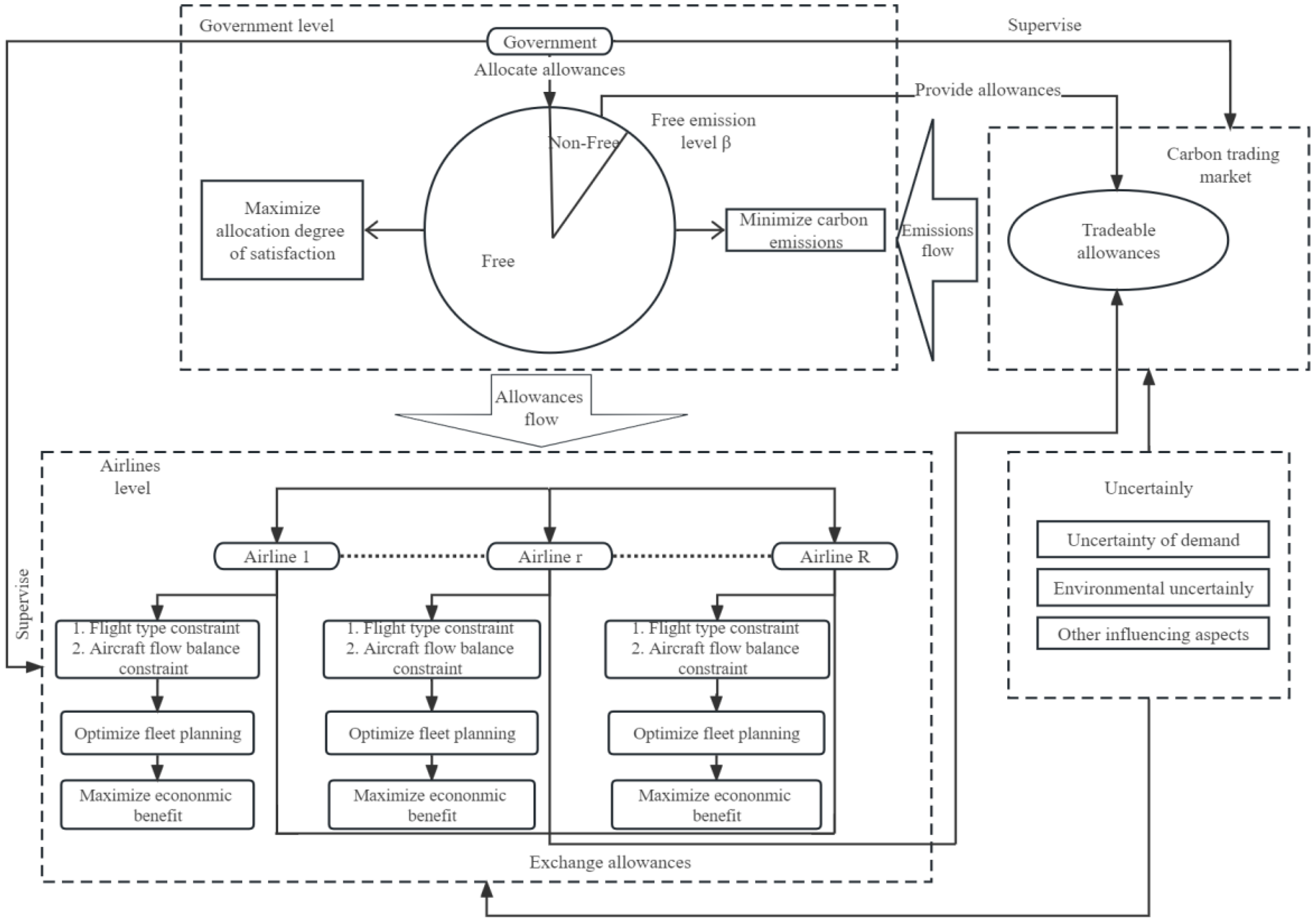Section 2 demonstrates an aviation-specific carbon trading mechanism and the game between the government and airlines. In Section 3, a bi-level programming model is developed to represent the game relationship between government demand for emissions reduction and airline fleet planning under the carbon trading mechanism. Section 4 presents a case study to review the applicability of the approach and provides insights for stakeholders in different scenarios. Finally, Section 5 concludes the paper.

2. Key Problem Statement

2.1. Carbon Emission Trading Process

Countries and organizations have introduced various systems to reduce carbon emissions, such as the European Union Emissions Trading Scheme (EU-ETS) and the Carbon Offsetting and Reduction Scheme for International Aviation (CORSIA). The carbon trading system is considered to be the most effective incentive mechanism [23]. As the first platform to regulate and commercialize carbon emissions in commercial aviation [24], the EU-ETS has become a standard model for carbon trading systems in other countries and regions [25].

China’s carbon trading system is currently only implemented in the power industry [26] and has proved obvious effectiveness [27]. To this point, this paper presents an aviation-specific emissions trading scheme involving the take-off and landing emissions from all flights. Past studies have shown that the maximum expandable profit and carbon emission reduction for airlines could be achieved simultaneously under the carbon trading system [28]. Analogous to traditional carbon trading mechanisms, the airline will sell the excess credits if the allocated free carbon credits are not fully utilized, and the credits are stored in a government-regulated carbon bank. Conversely, airlines must buy extra carbon allowances on the government-managed carbon market if their actual emissions exceed the allocated free allowances [29]. The government allocates free and non-free carbon credits to each airline, which means that the government sets a cap on the total carbon emissions of airlines depending on their performance, and this limit is designed to prevent a significant increase in unusual price volatility in the carbon market [30]. For example, if airline A intends to sell carbon allowances, then the allowances will be stored in the carbon bank, and airline B can purchase carbon allowances from this bank when the allocated credits do not cover its operational demand. This will force airlines to adjust their fleets under environmental regulations. Meanwhile, the system makes fleet planning an effective way to resolve conflicts between the government and airlines. The government will adjust the allocated carbon credits depending on airlines’ carbon emission performance. Once an airline adopts a fleet plan with higher carbon intensity, the government may arrange fewer free carbon credits. The airline also has to purchase carbon emissions in the carbon trading market. This will result in higher costs for the airline and lead airlines to optimize fleet composition, finally achieving the carbon reduction targets.

As shown in Figure 1, the government allocates free carbon credits to airlines by reference to their original carbon emission levels. The fleet plan is developed by the airlines based on the allocated free carbon credits, passenger demand, routing, and other factors. Airlines’ carbon emissions are to be reported to governments, and governments adjust the airline’s allocated free carbon credits based on the projected carbon emissions. This process coordinates the carbon reduction targets and economic profit until a final equilibrium is obtained.

2.2. The Game between Government and Airlines Based on the Emissions Trading Mechanism

Under the emissions trading scheme concept described above, the governments design the amount of free and creditable carbon allowances allocated to the airlines based on their carbon emissions, taking into account the total number of carbon emissions and the airline’s satisfaction. Airlines seek higher operating profit and aim to acquire more free carbon credits to expand their operations and thus increase revenues, but actions such as increasing the number of passengers and using aircraft with more seats will result in more actual carbon emissions, which will cause the government to reduce the number of free carbon credits allocated. In addition, buying large amounts of carbon credits will also raise the transaction price in the carbon market, making airline operations less profitable. So, airlines design fleets based on the carbon credits allocated and present the fleet plan and carbon emissions to the government. The governments then adjust the number of carbon allowances allocated to the airlines depending on their new carbon emissions. When the cycle ends, airlines will stick to the fleet planning they submitted to the government.

Each airline is an independent decision maker and desires to increase its profit. They can buy carbon credits or sell excess credits in the market and construct the appropriate fleet based on the government’s carbon credit allocation, routing, and passenger travel requirements. The selection can also in turn affect the number of carbon emissions allocated by the governments. In this way, a “leader–follower” relationship is created between the government and these airlines.

In summary, the carbon trading mechanism in the airline industry is a game between the government and the airlines. In this system, the government takes a dominant role in trying to minimize total carbon emissions and maximize airline satisfaction based on airlines’ initial fleet plans and total carbon emissions. Airlines adjust their fleet composition and buy or sell carbon credits based on the allocated credits to maximize their economic benefits.

3. Methodology

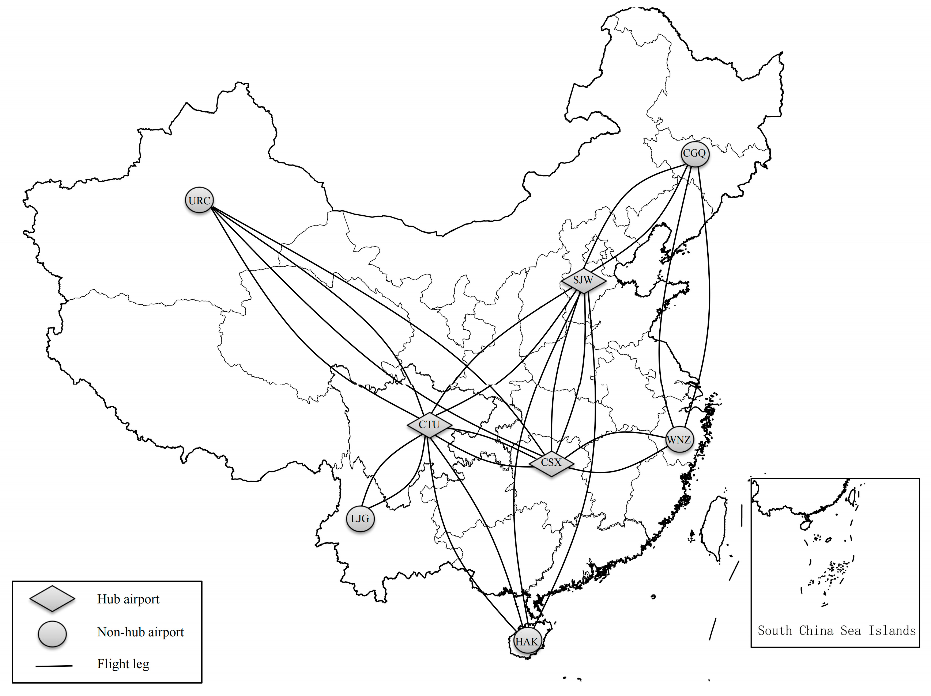
Therefore, this paper obtains the fleet size and composition by means of assigning aircraft types to the given flight schedule based on the time-and-space network, so as to reflect this interaction between government emissions reduction demand and airline fleet planning. The advantages of using the time-and-space network lie in the fact that (1) it solves the problem that the traditional macro fleet planning method cannot reflect the technical and economic adaptability of specific aircraft types on flights, (2) it can better capture the passenger spilling effects (a passenger spilled from a flight leading to the passenger’s disappearance on its connecting flight) in the hub-and-spoke network, and (3) it can clearly depict the relationship between government carbon quota allocation, carbon emission trading pricing, and airline fleet size and structure.

3.1. Problems and Assumptions

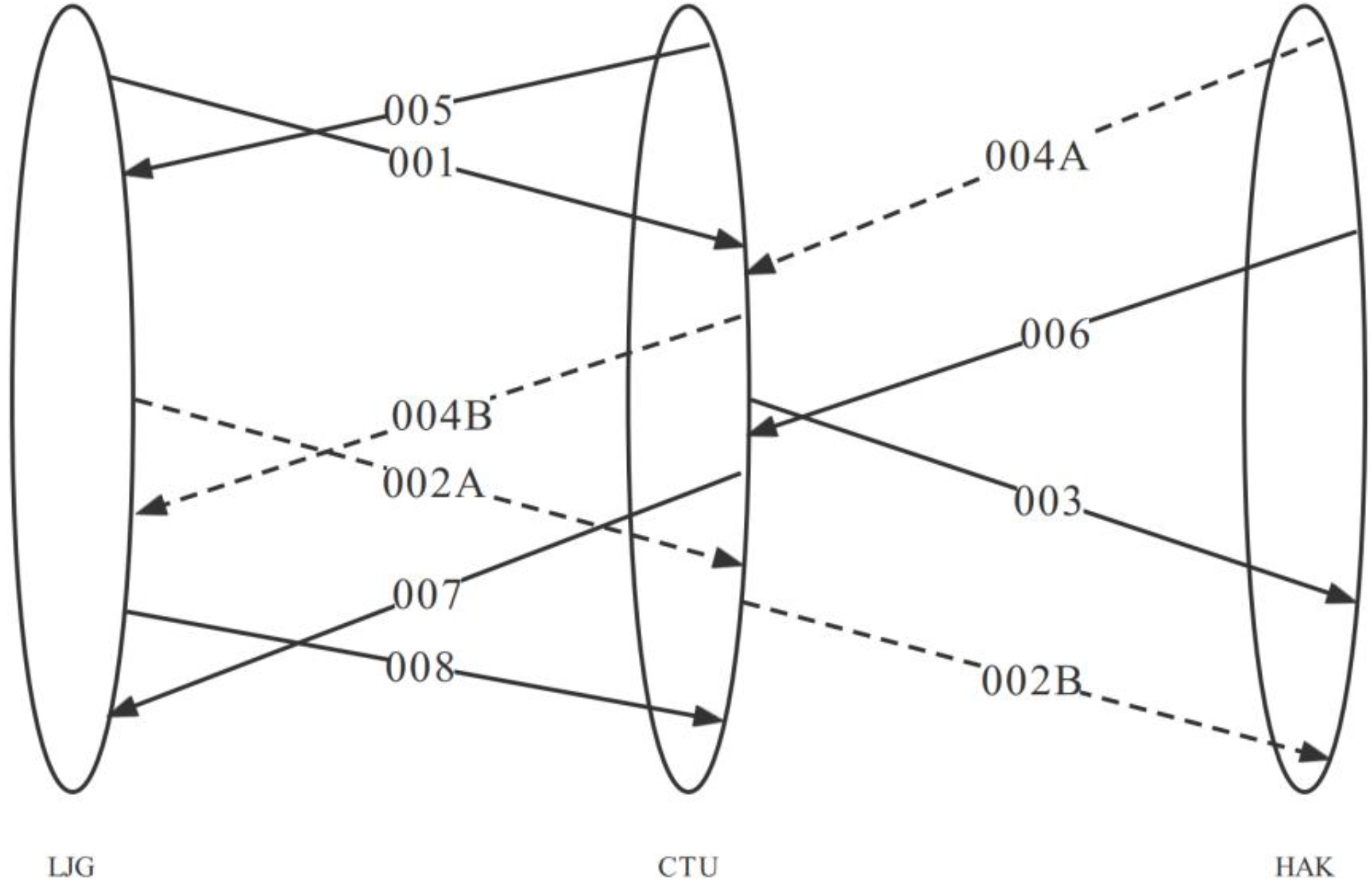
The path chosen by a passenger from the point of origin to the destination is defined as an itinerary, and each itinerary consists of one or more flights. To simplify the calculation, this paper assumes that passenger demand is independent of each itinerary [31]. The number of passengers in a real case study is used to estimate the level of demand on each travel structure, and the remaining demand on each flight is ignored. Although some details are simplified in this paper, the approach followed the basic practice of the airline industry.

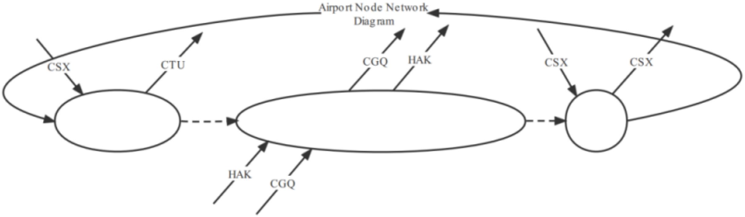
The operating cycle is defined as the period in which all flights of a typical daily schedule occur (i.e., a natural day). Figure 2 shows an airport in Shijiazhuang. In this period, departure and completion events are defined according to the departure and earliest completion times of all flights. For each airport, the successive completion events and departure events are considered as the same node, and all events are divided into different nodes in different airports. The first consecutive departure event is considered as the first node, and the last consecutive completion event is considered as the last node. Although the number of arriving and departing aircraft at each node is not necessarily the same, the number of departing aircraft at the first node is equal to the number of arriving aircraft at the back node for each airport.

According to the carbon emissions trading scheme mentioned in Chapter 2, the following assumptions are adopted to construct a time-and-space-network-based bi-level model for the airline green fleet planning method: (1) If provided allowance does not match actual emissions, airlines sell or purchase the credits on the carbon trading market. (2) In the process of the game between the governments and the airlines, free allowances and non-free carbon credits are reset according to the airline’s total carbon emissions in the last cycle (the rationality of both assumptions 1 and 2 can be referred to the literature [32] for details). (3) Information such as fleet configuration, routes, carbon emissions, etc. are all accurately obtained by the government. In practice, the airline’s operations are closely regulated by the government. This assumption suggests that all parties know all the information at the time of decision making. This assumption is consistent with the one in reference [33] for the game problem. (4) Several parameters including demand level, variable operating costs, and fixed costs are considered uncertain; they represent the uncertain operating environment which is widely used in fleet planning methods [34,35,36].

Assuming that airlines aim to maximize their operating profit, the operating revenue of route i can be expressed as the product of the demand for that flight and the fare. The corresponding function is shown in Equation (1):

$${\mathrm{revenue}}_i=\mathrm{fare}\hspace{0.33em}{\mathrm{price}}_i\times {\mathrm{demand}}_i$$

(1)

Airlines’ total costs are divided into fixed costs, variable costs, and emission-related costs. Fixed costs include maintenance costs, labor costs, and depreciation costs, which are considered to be billable on a daily basis. Variable costs are mainly fuel costs, depending on the number of passengers carried by the aircraft and the route flown. Therefore, the operating cost is calculated as shown in Equation (2).

$$\mathrm{COST}=\mathrm{fixed}\hspace{0.33em}\mathrm{cost}+\mathrm{variable}\hspace{0.33em}\mathrm{cost}+\mathrm{carbon}\hspace{0.33em}\mathrm{cost}$$

(2)

Minimizing carbon emissions is one of the government’s goals. To simplify the analysis, the carbon emissions from an aircraft waiting and taxiing on the ground during full braking are considered to be zero [37]. With the itinerary demand determined, the carbon emissions of the flight are calculated as follows.

$${\mathrm{Emission}}_i=F(X_{ik}(r),{\delta }_{ij}{s}_j(r))$$

(3)

where $X_{ik}(r)$ indicates flight $i$ with aircraft type $k$, and ${\delta }_{ij}{s}_j(r)$ is the number of passengers in flight $i$.

In 2014, the International Civil Aviation Organization (ICAO) published a method for calculating carbon emissions [38]. Referring to this method and other theoretical studies [39], the method used in this work to calculate carbon emissions is presented in Equation (4).

$$\begin{array}{l}F(X_{ik}(r))=3.157\times M_{fuel}\times (\mathrm{aircraft}\hspace{0.17em}\mathrm{bare}\hspace{0.17em}{\mathrm{weight}}_k\hspace{0.33em}+\hspace{0.33em}\hspace{0.33em}50\hspace{0.33em}\times \hspace{0.33em}{\mathrm{seat}}_i\hspace{0.33em}\\ \hspace{1em}\hspace{1em}\hspace{1em}\hspace{1em}\hspace{1em}+100\hspace{0.33em}\times \hspace{0.33em}(\mathrm{load}\hspace{0.33em}\mathrm{factor}\hspace{0.33em}\times \hspace{0.33em}\mathrm{number}\hspace{0.33em}\mathrm{of}\hspace{0.33em}{\mathrm{seats}}_k))\end{array}$$

(4)

where $M_{fuel}$ is the fuel coefficient as shown in Equation (5).

$$M_{fuel}=[1-e^{-\frac{{\mathrm{dis}}_i\times {\mathrm{ratio}}_{cr}{}^k}{10\times v_k}}]$$

(5)

In the carbon trading mechanism, the carbon price consists of an initial carbon trading price (i.e., $q$) and a fluctuating carbon trading price [40]. Supply and demand fluctuations are calculated by multiplying the volatility factor (i.e., $Q$) by the trading volume in the carbon trading market (i.e., $Q{\displaystyle \sum _{r\in R}{M}_P(r)}$). For airlines, the price of carbon credits is positively related to the number of carbon credits purchased. Thus, the carbon trading price can be expressed as Equation (6).

$$TC=q+Q{\displaystyle \sum _{r\in R}{M}_P(r)}$$

(6)

3.2. Model Formulation

Different passenger demands within the route network are divided into different scenes, r. The illustration of sets, indices, parameters, and decision variables in the formulations are presented in Appendix A (

Table A1. Notations for the proposed model.

Sets and indices	Description
$I$	Set of flight legs, indexed by i;
$J$	Set of passenger itineraries, indexed by j;
$K$	Set of aircraft types, indexed by k;
$V$	Set of airports, indexed by v;
$T$	Set of departure and arrival nodes, indexed by t;
$R$	Set of scenes, indexed by r;
$IN(k,v,t)$	Set of flight legs into airport v, flown by aircraft type k which arrive at node t;
$OUT(k,v,t)$	Set of flight legs into airport v, flown by aircraft type k which depart at node t;
Parameters	Description
$TC$	Price of carbon on the carbon trading market;
$p_j$	Passenger fare in itinerary j;
$n_j(r)$	Travel demand in itinerary j in scene r;
$C_{ik}$	Variable costs for flights i operated by aircraft type k;
$A_k$	Fixed costs by aircraft type k;
${\delta }_{ij}$	Binary variables, where ${\delta }_{ij}$ is equal to 1 if itinerary j is assigned to leg i;
$Ca{p}_k$	Capacity of aircraft type k;
$G_{ik}(r)$	The emissions from flight leg i by aircraft type k in scene r;
$h_i$	The length of the air route i;
${\mathrm{dis}}_i$	The cruising distance of flight i;
${\mathrm{ratio}}_{cr}{}^k$	The quotient of the fuel consumption ratio and the lift-drag ratio;
$v_k$	The cruising speed of aircraft type k;
$\mathrm{aircraft}\hspace{0.17em}\mathrm{bare}\hspace{0.17em}{\mathrm{weight}}_k$	Variable costs for flights i operated by aircraft type k;
$\mathrm{load}\hspace{0.33em}\mathrm{factor}$	A ratio of the enplaned passenger on an airplane to the airplane seat capacity;
$\mathrm{number}\hspace{0.33em}\mathrm{of}\hspace{0.33em}{\mathrm{seats}}_k$	The rated seat capacity of aircraft type k;
${\mathrm{seat}}_i$	The actual number of passengers on flight i;
Decision variables	Description
$M_F(r)$	The free allowances from the government in scene r;
$M_P(r)$	The non-free allowances from the government in scene r;
$X_{ik}(r)$	Binary variable; 1 denotes that aircraft type k is selected of the air route i in scene r, otherwise 0;
${\mathrm{y}}_{kvt-}(r)$	The Number of aircraft type k on the ground at airport v drive into node t in scene r;
${\mathrm{y}}_{kvt+}(r)$	The number of aircraft type k on the ground at airport v depart from node t in scene r;
$s_j(r)$	The number of passengers for itinerary j in scene r;
$Z_k(r)$	The number of aircraft type k in the fleet in scene r.

).

• Minimize carbon emissions: The cap of carbon emission allowances in scene r is allocated into the free allowances (i.e., $M_F(r)$) and non-free allowances (i.e., $M_P(r)$). The airline’s carbon emissions can be expressed as the sum of the free credits and trading credits allocated to the airline by the government, which can be seen in Equation (7).

  $$U(r)=M_F(r)+M_P(r)$$

  (7)

  where $U(r)$ is the carbon emissions of airline in scene r.
• Allocation degree of satisfaction: The multi-objective optimization aims to obtain a set of trade-off solutions between contradictory objectives (carbon emissions and satisfaction) by adjusting free allowances. The allocation satisfaction of airlines reflects the airlines’ attitude toward the government, which is dependent on the number of free carbon allowances allocated to airlines by the government. In the upper layer, the objective function of satisfaction is set to the quotient of $M_F(r)$ and $ACG(r)$. The more free carbon allowances an airline receives, the higher the allocation satisfaction [41]. The allocation degree of satisfaction for each airline is defined as Equation (8).

  $$Y(r)=\hspace{0.17em}\frac{M_F(r)}{ACG(r)\hspace{0.17em}}$$

  (8)

  where $Y(r)$ is the degree of satisfaction of airline, and $ACG(r)$ is the actual carbon emissions of airline in scene r.
• Allocation of carbon credits by the government: As the policy maker in the field of carbon emission allowances, the main question for the government is how to achieve emissions reduction targets [42]. The government makes decisions based on its carbon reduction requirements and the airline’s total carbon emissions from the previous cycle. This leaves the percentage of the free allowances in scene r to the total allocated allowances to $\beta (r)$. This ratio is based on the airline’s carbon emissions in the previous year and the government’s reduction target [43].

  $$\beta (r)=\frac{M_F(r)}{M_F(r)+M_P(r)}$$

  (9)
• Demand constraints: To ensure the operation of airlines, the free allowances allocated to airlines (i.e., $M_F(r)$) cannot be less than their minimum requirement to operate all flights (i.e., $d_{\min }(r)$). This demand is based on the airline’s flight schedule and passenger demand from the previous cycle, the mathematical expression can be seen in Equation (10).

  $$M_F(r)\ge d_{\min }(r)$$

  (10)
• Airlines’ aircraft selection plan: The government’s goal is to minimize the carbon emissions of all airlines, so the free carbon allowances that the government allocates to each airline are lower than their original carbon emission. Therefore, airlines must maximize their economic efficiency by adjusting their fleet planning options based on the number of carbon credits allocated.
• Economic benefit: Airlines’ revenue comes from the sale of carbon credits and ticket sales. The airfare revenue of aircraft type k in flight leg i in scenario r is calculated from the airfare for aircraft type k multiplied by the number of seats for itinerary j. If airlines do not fully use the free emission allocation allocated by the government, they may sell them. Airlines may also purchase additional emission credits if the free credits allocated to them do not meet their needs. For different airlines, the amount of carbon traded by the airline may equal either the number of carbon allowances sold or the number of carbon allowances purchased, so the product of the amount of carbon traded and the price of carbon may represent both costs and revenues. Fleet operating costs consist of variable operating costs (i.e., $C_{ik}$) and fixed costs (i.e., $A_k$). The variable operating cost per aircraft is called the variable cost, which is the variable cost of operating flight i with aircraft type k and is positively related to flight duration. The fixed cost is the average acquisition cost of the aircraft type k. Considering the effect of uncertainty, the airfare and the operating cost are set as fuzzy random parameters. Therefore, the operating benefit function for an airline in scenario r can be transformed as Equation (11). It should be noted that the costs mentioned in this paper must be directly related to the aircraft types and the accounting policy, economics, and aircraft utilization rate, which differ among countries around the world. So, the profit presented in this paper does not represent the net income of the airline.

  $$\max f(r)={\displaystyle \sum _{j\in J}{p}_j{s}_j(r)-}{\displaystyle \sum _{i\in I}{\displaystyle \sum _{k\in K}{X}_{ik}}}(r)C_{ik}-TC\times M_P(r)-{\displaystyle \sum _{k\in K}{A}_k{Z}_k(r)}$$

  (11)

The number of carbon trading for airline (i.e., $M_P(r)$) depends on the value of the difference between free allowances and actual emissions (i.e., ${\displaystyle \sum _{i\in I}{\displaystyle \sum _{k\in K}{X}_{ik}(r)G_{ik}(r)}}$). The mathematical expression can be seen in Equation (12).

$$M_P(r)={\displaystyle \sum _{i\in I}{\displaystyle \sum _{k\in K}{X}_{ik}(r)G_{ik}(r)}}-M_F(r)$$

(12)

The change in revenue for airline in scenario r due to the sale or purchase of carbon credits is denoted as $COS{T}_C(r)$, as shown in Equation (13).

$${\mathrm{COS}\mathrm{T}}_C(r)=TC\times M_P(r)$$

(13)

7.

Aircraft number constraints: To allow for the consistent management of aircraft, airlines must ensure that the overnight airport remains the same for each aircraft. The number of type k aircraft flying to the first node at each airport is equal to the number of type k aircraft flying to the last node at that airport, as shown in Equation (14). At the first node, the number of aircraft of a type waiting for orders at all airports is equal to the number of aircraft of that type in the fleet. This mathematical expression is shown in Equation (15).

$${\displaystyle \sum _{v\in V}{y}_{kv,t^{-}=1}(r)=}{\displaystyle \sum _{v\in V}{y}_{kv,t^{+}=last}(r)},\forall k\in K,r\in R$$

(14)

$$Z_{\mathrm{k}}(r)={\displaystyle \sum _{v\in V}{y}_{kv,t^{-}=1}}(r) \forall \mathrm{k}\in K,r\in R$$

(15)

where $Z_k(r)$ is the number of aircraft of type k in scenario r, ${\displaystyle \sum _{v\in V}{y}_{kv,t^{-}=1}}(r)$ is the number of departures in scenario r in the network at the first node in airport v, and ${\displaystyle \sum _{v\in V}{y}_{kv,t^{+}=last}}(r)$ is the number of aircraft of in scenario r at the last node within airport v.

8.

Aircraft selection constraints: Once the fleet plan is established, the flight type assignment must meet the requirement of uniqueness. For each airline, only one type of aircraft can be selected on the air route in scenario r, as shown in Equation (16).

$${\displaystyle \sum _{\mathrm{k}\in K}{X}_{ik}(r)}=1,\forall \mathrm{i}\in I,r\in R$$

(16)

9.

Aircraft flow balance constraints: To optimize the utilization of aircraft, airlines must minimize the number of unused aircraft at airports. In scenario r, the number of aircraft of a type entering a node at any airport must be equal to the number of aircraft of the same type leaving that node, as shown in Equation (17).

$$\begin{array}{c}{\displaystyle \sum _{r\in R}{\mathrm{y}}_{kv{t}^{-}}(r)}-{\displaystyle \sum _{r\in R}{\mathrm{y}}_{kv{t}^{+}}(r)}+{\displaystyle \sum _{i\in IN(k,v,t)}{X}_{ik}(r)}-{\displaystyle \sum _{i\in OUT(k,v,t)}{X}_{ik}(r)}=0,\\ \\ \forall k\in K,v\in V,t\in T\end{array}$$

(17)

where ${\mathrm{y}}_{kvt-}(r)$ is the number of aircraft of the type k driving into node t in airport v, ${\mathrm{y}}_{kvt+}(r)$ is the number of aircraft of type k departing to node t in airport v, ${\displaystyle \sum _{i\in IN(k,v,t)}{X}_{ik}(r)}$ is the number of aircraft of the type k arriving at the airport v in node t, and ${\displaystyle \sum _{i\in OUT(k,v,t)}{X}_{ik}(r)}$ is the number of aircraft of the type k departing to the airport v in node t.

10.

Passenger flow constraints: For each airline, the number of seats allocated on each flight leg in scene r (i.e., $s_j(r)$) does not exceed the total number of seats for that aircraft type k (i.e., $Ca{p}_k$). At the same time, the number of seats provided for itinerary j (i.e., $s_j(r)$) is within the passenger demand in that itinerary (i.e., $n_j$). These mathematical expressions are shown in Equations (18) and (19).

$${\displaystyle \sum _{j\in J}{\delta }_{ij}{s}_j(r)\le {\displaystyle \sum _{k\in K}{\displaystyle \sum _{r\in R}Ca{p}_k{X}_{ik}(r)}}},\forall i\in I$$

(18)

$$0\le s_j(r)\le n_j \forall j\in J$$

(19)

11.

Fleet consistency constraints: For each scenario r, the optimal fleet planning may differ between different demand scenarios. Fleet planning is a long-term decision that means an airline cannot simply change the structure of its fleet at short notice. Therefore, the fleet planning obtained should combine all scenarios and be appropriate for the entire planning cycle. As shown in Equation (20), the fleet in different scenes r is restricted to the same as the program variables (i.e., ${\overline{Z}}_k$); it represents the fleet planning obtained by integrating all scenarios.

$$Z_k(r)={\overline{Z}}_k,\forall k\in K,r\in R$$

(20)

According to the government’s carbon emission limits and the airline’s operation conditions, this paper establishes a two-tier decision-making structure, with the government as the upper decision maker and the airlines as the lower decision maker. In the allocation decision, the government first considers the minimization of total carbon dioxide emissions while pursuing the goal of maximizing the satisfaction of airlines and ensuring the normal operating activities of airlines. Therefore, the upper-level objective function is set to minimize the sum of free carbon credits and traded carbon credits and maximize airline satisfaction simultaneously.

In the enterprise operation decision, airlines tend to create the most favorable fleet plan with the time-and-space networks to maximize the profit. This process is regulated by governments and takes into account the random nature of demand. If airlines are not allocated enough free carbon credits, they will buy additional credits in the carbon trading market. If the government allocates too many free carbon credits, the airline will sell the excess carbon credits in the trading market. The carbon allowances allocated by the government directly affect the airlines’ operation and fleet planning, and the airlines’ specific fleet planning in turn affects the government’s carbon emissions reduction target.

Based on the above analysis, the fleet planning approach for passenger aviation has the ability to resolve the conflict between the government and airlines over aviation demand and carbon emissions reduction, and a trade-off can be achieved, eventually. To describe this relationship, this paper formulates the problem as a global model with a two-layer structure. The mathematical expression is shown in Equation (21).

The decision variables of the government (i.e., free allowances $M_F(r)$ and non-free allowances $M_P(r)$) are first initialized. Seeking solutions at the government level starts from the initialization and must meet the constraints (i.e., Equations (9) and (10)) to guarantee feasibility. Combining carbon savings targets and satisfaction targets, the free allowances and non-free allowances are formulated by the government in the first round of negotiations simulation. A new fleet plan is generated under the constraints (i.e., Equations (14)–(20)) at the airline level from the decision variables, and these carbon emissions serve as feedback to the government level. If the generated fleet scenario is the same as the scenario in the previous simulation, the gaming process of the simulation will be interrupted. Otherwise, a new round of simulated negotiation will begin. The government adjusts the decision variables based on these carbon emissions and sends them to the airline; the airline will then design a new fleet planning in this round of simulations. The cycle continues until the termination condition is met. Note that the whole negotiation is a simulation of the decision-making process, and only the final decision of carbon allowances and fleet composition is implemented, where the upper level (government) and lower level (airline) get feedback several times and achieve a final equilibrium strategy.

4. Results and Discussion

A numerical example is given in this section to demonstrate practicability and effectiveness. Actual production and operational data from a typical daily flight schedule of a major hub and network airline are used as basic data. Using these data, an improved fleet plan is constructed and the impact of different factors on the fleet plan is discussed.

$$\left\{\begin{array}{c}\underset{M_F\left(r\right)}{\min U\left(r\right)}=M_F\left(r\right)+M_P\left(r\right)\hfill \\ \underset{M_F\left(r\right)}{\max Y}=\frac{M_F\left(r\right)}{ACG\left(r\right)}\hfill \\ \beta \left(r\right)=\frac{M_F\left(r\right)}{M_F\left(r\right)+M_P\left(r\right)}\hfill \\ M_F\left(r\right)\ge d_{\min }\left(r\right),\forall r\in R\hfill \\ \mathrm{s}.\mathrm{t}.\left\{\begin{array}{c}\max f\left(r\right)={\displaystyle \sum _{j\in J}}{p}_j{s}_j\left(r\right)-{\displaystyle \sum _{i\in I}}{\displaystyle \sum _{k\in K}}{\displaystyle \sum _{r\in R}}{X}_{ik}\left(r\right)C_{ik}-TC\times M_P-{\displaystyle \sum _{k\in K}}{A}_k{Z}_k\left(r\right)\hfill \\ \mathrm{s}.\mathrm{t}.\left\{\begin{array}{c}{\displaystyle \sum _{\mathrm{k}\in K}}{X}_{ik}\left(r\right)=1,\forall i\in I,r\in R\hfill \\ G\left(r\right)={\displaystyle \sum _{i\in I}}{\displaystyle \sum _{k\in K}}{\displaystyle \sum _{j\in J}}F\left(X_{ik}\left(r\right),{\delta }_{ij}{s}_j\right),\forall r\in R\hfill \\ TC=p+Q{\displaystyle \sum _{r\in R}}{M}_P\left(r\right)\hfill \\ y_{kvt-}\left(r\right)-{\mathrm{y}}_{kvt+}\left(r\right)+{\displaystyle \sum _{i\in IN(k,v,t)}}{X}_{ik}\left(r\right)-{\displaystyle \sum _{i\in OUT(k,v,t)}}{X}_{ik}\left(r\right)=0,\hfill \\ \forall k\in K,v\in V,t\in T,r\in R\hfill \\ {\displaystyle \sum _{v\in V}}{y}_{kv,t^{-}=1}\left(r\right)={\displaystyle \sum _{v\in V}}{y}_{kv,t^{+}=las}\left(r\right),k\in K,r\in R\hfill \\ {\displaystyle \sum _{j\in J}}{\delta }_{ij}{s}_j\left(r\right)\le {\displaystyle \sum _{k\in K}}{Cap}_k{X}_{ik}\left(r\right),\forall i\in I,j\in J,r\in R\hfill \\ Z_{\mathrm{k}}\left(r\right)={\displaystyle \sum _{v\in V}}{y}_{kv1-}\left(r\right),\forall k\in K,r\in R\hfill \\ 0\le s_{jk}\left(r\right)\le n,\forall j\in J\hfill \\ X_{\mathrm{ik}}\left(r\right)\in \{0,1\},\forall i\in I,k\in K,r\in R\hfill \\ Z_{\mathrm{k}}\left(r\right)\ge 0,\mathrm{int},\forall k\in K\hfill \\ y_{kvt-/+}\left(r\right)\ge 0,\mathrm{int},\forall k\in K,v\in V,t\in T,r\in R\hfill \\ s_j\left(r\right)\ge 0,\mathrm{int},\forall j\in J\hfill \\ Z_k\left(r\right)={\overline{Z}}_k,\forall k\in K,r\in R\hfill \end{array}\right.\hfill \end{array}\right.\hfill \end{array}\right.$$

(21)

4.1. A Hub-and-Spoke Case Presentation

A hub-and-spoke route network including 8 sectors, 43 flights, and 62 routes is selected as the numerical example. As shown in Figure 3, the route network is a hub-and-spoke route network where Chengdu (CTU), Changsha (CSX), and Shijiazhuang (SJW) airports serve as hubs. In addition, five non-hub airports are selected, including Lijiang (LJG), Urumqi (URC), Haikou (HAK), Wenzhou (WNZ), and Changchun (CGQ) airports, and each non-hub airport differs in passenger demand. Those routes involve situations between the non-hub airport and the hub airport as well as the non-hub airport and another non-hub airport. The demand is considered an independent parameter and yields to the normal distribution. Passenger demand in this case is divided into r scenes to account for the randomness of demand on the network, which was estimated based on the following procedure.

(1)

Let the demand on each itinerary j (j = 1, 2, …, J) yield to the normal distribution $d_j~N({\mu }_j,{\sigma }_j)$ with cumulative probability distribution function $F_j$.

(2)

Specify the number of scenarios to be generated (denoted by R).

(3)

Set the value of R equally spaced quantiles of the distribution j $(d_j[1],d_j[2],\cdots d_j[R])$ so as to generate more values from a range with a higher density of distribution and fewer values from low-density regions.

(4)

Generate each vector $(d_1[r],d_2[r],\cdots d_J[r])$ by randomly permuting of the values $d_j$ for each itinerary, which represents a scene that includes all itineraries.

(5)

Combine all vectors into a 5000 × 62 matrix, where each row vector represents a scene, and each column vector corresponds to the demands of an itinerary in all scenes.

Figure 4 gives an example of the itineraries in the hub-and-spoke network. There are three airports, located in Lijiang, Chengdu, and Haikou, respectively. These legs are denoted by the flight code, such as 002A. Itineraries consist of multiple flight legs, starting with numbers and followed by an alphanumeric character. Take the 002A for example, the 002 is the second itinerary among all the trips of the day, and the A indicates the leg is the first in this itinerary. The solid line indicates that the trip has only one section of travel, and the dashed line means the itinerary consists of multiple flight legs. According to the flight code in Figure 4, 002A and 002B were part of one itinerary because their arrival and departure time points at CTU airport are successive.

Different aircraft are assumed to be available on the same route segment between two airports. For instance, although flight legs 001 and 005 form a round trip, these flight legs can only be operated with two aircraft due to scheduling conflicts. Different airlines have different average amounts of annual passenger demand for the same itinerary, so this paper uses the average passenger demand of all airlines on each itinerary as the demand for that route. Similarly, the airfares of all airlines for each route structure are obtained, and the average of the airfares is used as the base price for that route structure.

Six on-duty aircraft types are considered: A320, A330, A340, B767, B737, and B777. The airlines can choose from these six appropriate aircraft types to serve the routes. The basic information about these aircraft, such as the number of passenger seats, empty weight, cruise speed, ratio, hourly operating cost, and unit acquisition cost, is shown in

Table 1. Basic information of these aircraft types.

Aircraft Type Index k	Description
	A320	A330	A340	B767	B737	B777
Number of passenger seats	156	334	324	226	194	361
Weight (kg)	142,400	229,600	229,000	180,127	160,000	239,225
Cruising speed (km/h)	852	896	896	851	796	905
Lift–drag ratio	0.327	0.296	0.288	0.356	0.201	0.297
Operating costs (CNY/h)	34,000	65,000	62,000	43,000	40,000	68,000
Unit purchase cost (CNY)	40,000	70,000	70,000	50,000	48,000	76,000

, which was collected from the International Civil Aviation Organization (ICAO) [44]. In managing the aircraft fleets, the commercial airline inevitably has to take into account the uncertainty of costs and airfare. In this study, the airfare for itinerary j (i.e., $p_j$), costs for flights I operated by aircraft type k (i.e., $C_{ik}$), and fixed costs by aircraft type k (i.e., $A_k$) are not fixed because of various uncertain elements. Therefore, these parameters are regarded as uncertain parameters, and fuzzy random variables are used to model the statistical data in this study, which were estimated based on the following procedure: (1) For each flight, actual production and operational data of a major hub and network airline are used to conduct an investigation with each giving ranges. (2) The lower bound of the fuzzy random variables is set to a minimal value for all groups. (3) The upper bound of the fuzzy random variables is set to a maximal value for all groups. (4) The parameters are assumed to approximately follow normal distributions and the expected value is estimated. (5) The expectations and all fuzzy random variables (i.e., $p_j$, $C_{ik}$, $A_k$) are determined.

For the carbon trading market, the carbon price is influenced by the initial price and the carbon purchase volume, as shown in Equation (6). The initial price of carbon is set to 50 CNY/ton and the volatility factor is set to 0.1. This is derived from some mature aviation carbon trading markets, current carbon trading prices and carbon growth rates in domestic carbon trading markets [45,46].

4.2. Operation Results and Analysis

To show the effectiveness of the fleet planning method proposed in this paper, the fleet assignment optimization environment was implemented in Python 3.8 paired with the Gurobi Optimizer. The key was to find a fleet plan that satisfies both the government and the airlines. First, the scenario that best meets the requirements of the interests of both parties was selected as the base case. Various sensitivity analyses were then performed on the trade-off between operating profit and carbon emissions, free carbon emission levels, and carbon trading market parameters.

Table 2. The scenarios for further analysis.

Scenario	Objective	Passenger Demand Level	Carbon Trading Price
S1 *	First: minimize carbon emissions; second: maximize profit	100%	50 CNY/ton
S2	Single objective (profit maximization)	100%	-
S3	First: minimize carbon emissions; second: maximize profit	160%	50 CNY/ton
S4	First: minimize carbon emissions; second: maximize profit	100%	100 CNY/ton

* Note that S1 is the baseline scenario.

shows the summary of all outlined scenarios. The results in each scenario were validated and compared to the base case results, which include economic, environmental, fleet, and market statistics, as well as some optimization statistics. All experiments described in this paper were performed on a 64-bit machine featuring an AMD Ryzen 7 6800H CPU.

4.2.1. Baseline Scenario

The parameter (i.e., $ACG(r)$) in the upper-level model will change when the airlines give feedback on their carbon emissions to the government. The objective functions of the upper-level model consider the changes in total carbon emissions and the satisfaction index of airlines (i.e., Equations (7) and (8)), respectively. If only one objective is taken into account and the other objective is ignored, the optimal value of the target can be obtained. Thus, when only one government-level objective is considered, the maximum values of the two objectives can be obtained separately, which are denoted as $U_{\max }$ and $Y_{\max }$. The maximum value is used to normalize the two objective functions and for summing, as shown in Equation (22).

$$\frac{U}{U_{\max }}+\frac{Y}{Y_{\max }}=\omega$$

(22)

To choose a suitable value of ω, a scenario analysis (with a step size of 0.1) was performed to determine how to adjust the weight of the two objective functions. The ratio U/Y represents the government’s tradeoff between the two objectives. After the government allocates free carbon allowances (i.e., $M_F(r)$) and fee-based carbon allowances (i.e., $M_P(r)$) to the airlines in the lower tier of the model, the airline will obtain a specific fleet plan with Equation (11). The airlines give the carbon emissions generated by this fleet scenario to the upper layer until a balance is reached. The results of the runs with different values are shown in

Table 3. Scenario analysis for the objectives.

	$\mathit{\omega }$	MF	MP	U	Y	U/Y
1	0.5	457,417	114,354	0.3844	0.1156	3.3253
2	0.6	471,453	117,863	0.3953	0.2047	1.9311
3	0.7	485,798	121,450	0.4042	0.2958	1.3666
4	0.8	499,787	124,946	0.4154	0.3846	1.0801
5	0.9	513,755	128,438	0.4267	0.4732	0.9017
6	1.0	527,680	131,920	0.4383	0.5616	0.7804
7	1.1	541,599	135,399	0.4499	0.6500	0.6922
8	1.2	555,522	138,880	0.4616	0.7384	0.6251
9	1.3	569,479	142,369	0.4730	0.8270	0.5719
10	1.4	583,392	145,848	0.4846	0.9154	0.5294

. Both target U and target Y tend to rise as the value of the ω rises, which causes the free carbon allowance to rise with it. According to Equations (7) and (8), it is clear that the government and airlines have different sensitivities to free carbon allowances. When the free carbon allowances increase, the satisfaction Y rises faster than U, so its ratio U/Y will decrease with this increase. Compared with other scenarios, Scenario 4 effectively reflected the attitudes of the government. At this point, U/Y is close to 1, indicating that the dual objectives of the government are equally important when ω equals 0.8. Therefore, this scenario was used as the basic case for the subsequent discussion.

When $\omega$ is 0.8, the carbon trading equilibrium model mentioned above was adopted. After the game between the government and the airline, a fleet plan that satisfies both parties is obtained, and its specific fleet and related parameters are shown in

Table 4. Optimization results for the baseline scenario.

Aircraft Type	A320	A330	A340	B767	B737	B777
Amount	13	0	0	1	5	0
Economic Statistics			Passenger Statistics
Operating profit (CNY)		3,765,964	Daily passenger demand			4931
Normalized fleet profit (CNY/seat/km)		0.3276	Number of passengers carried			4537
Normalized fleet profit (CNY/pax/km)		0.4345	Passenger load factor (%)			62.12
Total cost (CNY)		4,709,500	Fraction of passenger carried (%)			92.01
Normalized fleet operating cost (CNY/seat/km)		0.4096	Fraction of passenger carried—nonstop (%)			79.22
Normalized fleet operating cost (CNY/pax/km)		0.5434	Fraction of passenger carried—connecting (%)			20.78
Environmental Statistics			Fleet Statistics
Carbon emission (kg)		527,763	Passenger-kilometer (km)			8,666,710
Normalized fleet emission (kg/seat/km)		0.0459	Seat-kilometer (km)			11,496,476
Normalized fleet emission (kg/pax/km)		0.0609	Seating capacity			7304

.

The optimization results (when $\omega$ = 0.8) are selected as the baseline scenario (S1). On this premise, decision makers begin to balance carbon emissions with airlines’ satisfaction. The free carbon credits allocated to the airline by the government are smaller than the original carbon emissions. With the aim of reducing carbon emissions, airlines endeavor to adjust their fleets to achieve maximum economic profit and ultimately reach equilibrium. At this point, the airline has exhausted its free emission quota and purchased as few allowances as possible in the carbon trading market. The airline chooses three types of aircraft (A320, B767, and B737) to form its fleet at the same time. In this baseline scenario, the A320 aircraft account for 68.42% of the total fleet number, the B737 aircraft account for 26.32% of the total fleet purpose, and other aircraft types only account for 5.26%. In addition, to verify the effect of uncertainty, actual production data was used to compare fleet planning under exactness and random parameters. As shown in

Table 5. Comparison results under different types of parameters.

Aircraft Type	A320	A330	A340	B767	B737	B777
Stochastic parameters	13	0	0	1	5	0
Deterministic parameters	12	0	0	3	4	1
Operating profit (CNY)			Total cost (CNY)
Stochastic parameters	3,765,964		Stochastic parameters			4,709,500
Deterministic parameters	3,549,988		Deterministic parameters			4,882,696
Carbon emission (kg)			Seating capacity
Stochastic parameters	527,763		Stochastic parameters			7304
Deterministic parameters	570,012		Deterministic parameters			7814

, it indicated the fleet based on deterministic parameters is inferior in benefits to the fleet that takes stochastic parameters into account, and the environmental performance is also not satisfactory. Therefore, it is necessary to design fleet planning with stochastic parameters.

4.2.2. Impact of Environmental Policy

To investigate the impact of the environmental policy on airline fleet, the case without a policy aiming at reducing carbon emissions is proposed in this part. All assumptions are the same as those presented in Chapter 3. The fleet construct and related parameters obtained in this case are shown in

Table 6. Optimization results for a scenario without environmental policies.

Aircraft Type	A320	A330	A340	B767	B737	B777
Amount	11	0	2	4	2	0
Economic Statistics			Passenger Statistics
Operating profit (CNY)		4,028,132	Daily passenger demand			4931
Normalized fleet profit (CNY/seat/km)		0.3108	Number of passengers carried			4817
Normalized fleet profit (CNY/pax/km)		0.4310	Passenger load factor (%)			59.94
Total cost (CNY)		5,066,300	Fraction of passenger carried (%)			97.69
Normalized fleet operating cost (CNY/seat/km)		0.3909	Fraction of passenger carried—nonstop (%)			79.28
Normalized fleet operating cost (CNY/pax/km)		0.5421	Fraction of passenger carried—connecting (%)			20.72
Environmental Statistics			Fleet Statistics
Carbon emission (kg)		649,322	Passenger-kilometer (km)			9,346,033
Normalized fleet emission (kg/seat/km)		0.0501	Seat-kilometer (km)			12,959,462
Normalized fleet emission (kg/pax/km)		0.0695	Seating capacity			8036

.

S2 (scenario without environmental policies) is when the decision makers do not place any emphasis on carbon reduction. As is presented in Table 6, the proportion of A320 aircraft in the fleet reaches 57.89%. Correspondingly, the proportion of B737 aircraft in the fleet is only 10.53%. The number of passengers reaches 4817 and the passenger load factor is 59.94% in S2. Compared to Table 4, the operating profit presents a trend of dramatic increase, reaching CNY 4,028,132, while carbon emissions showed an obviously analogous trend. The carbon emissions are 649,322 kg, which is increased by 23.03% from S1. This indicated that the fleet in S2 is more profitable than S1, but the expansion in carbon emissions is more significant. Therefore, it can be observed that carbon trading mechanisms can reduce the total carbon emissions of airlines while maintaining their economic profits. This indicates that when governments implement carbon trading mechanisms in the aviation industry, carbon emissions can be effectively controlled, and the percentage of carbon emissions reduction is greater than the percentage of reduction in airline’s profits.

To explore the impact of carbon emission reduction mechanisms on flights, the revenue and emissions of each flight are compared in S1 and S2. Figure 5 depicts the operating revenue of each flight in these scenarios. It can be seen that the operating revenue of most flights is similar in both cases. The maximum operating revenue is CNY 760,508, and the minimum is CNY 65,616. However, the revenues on individual routes in S1 are less than S2. The operation revenue on flight 29 is CNY 334,254 in S1, which is 20.80% lower than S2. The revenue from other routes also decreased, such as flight 11 and 26. It is indicated that the total revenue will reduce if the carbon trading mechanism is introduced, but it does not mean that the revenue of each flight is reduced. The airlines still have the opportunity to keep the revenue of highly profitable flights unchanged.

The carbon emissions of routes also differ in the two scenarios, as shown in Figure 6. The carbon emissions of some routes exceed 30,000 kg in S2, such as flight 22 and flight 37. Flight 22 has the most carbon emissions, at 47,656 kg. When environmental policy is involved, the carbon emissions of most routes decrease steadily. In general, the results of all routes are below 30,000 kg, and the total carbon emission is 527,763 kg, which is 11.56% lower than S2. Specifically, it is obvious that the carbon emissions of flight 22 have undergone a dramatic increase from 25,531 kg to 47,656 kg, and the maximum of all flights rises to 26,426 kg.

For the government, the obvious rise between S1 (527,763 kg) and S2 (649,322 kg) suggests the effectiveness of reducing carbon emissions in the air transportation industry through the carbon trading mechanism. This approach of fleet planning combined with a carbon trading mechanism allows airlines to maintain a certain level of operating profitability, so it would be reasonable to expect it to be accepted by the company.

For airlines, the contrast between S1 and S2 illustrates the possibility of reducing carbon emissions from a strategic perspective. Furthermore, the results show that this approach has the opportunity for airlines to maintain their competitiveness on the most profitable routes. This can help airlines maintain their interests while complying with government policies, achieving a “win–win” situation in terms of environmental and economic benefits. This is of great significance in today’s slow development of low-carbon aviation fuels.

4.2.3. Impact of Passenger Demand Level

The passenger load factor is 62.12% in S1, which denotes the fleet has the capacity to accommodate more passengers. To increase passenger demand, airlines tend to use aircraft with more seats or expand the fleet size. These measures cause potential negative influences on carbon emissions. In the airline transportation market, airlines capture passengers from the total market level, and with higher market demand, the airlines can adjust the aircraft type on each flight. To explore the change in passenger load factor and the fleet under a higher market, it is supposed that the passenger demand gradually climbs to 200% of the original level. The increase in passenger demand level means an increase in the total market demand, not only the demand of each airline. Because of the higher price elasticity, airlines are not inclined to increase prices for short-haul routes [47,48], so the airline ticket price level remains unchanged in this process.

The operational results with various passenger demand level at a 20% increase are shown in

Table 7. Operational results of various passenger demand level.

	Passenger Demand Level	Passenger Load Factor	Profit (CNY)	Emission (kg)	A320	A330	A340	B767	B737	B777
1	100%	62.12%	3,765,964	527,763	13	0	0	1	5	0
2	120%	69.04%	4,641,427	528,040	15	1	0	0	4	0
3	140%	75.88%	5,277,387	527,800	15	1	0	0	4	0
4	160%	79.01%	5,681,599	527,670	16	0	0	0	4	0
5	180%	84.53%	5,893,103	528,047	15	0	1	0	2	0
6	200%	90.79%	6,010,326	527,793	15	1	0	0	2	0

. When passenger demand rises, there is a significant improvement in airline profit from CNY 3,765,964 to CNY 6,010,326. With the enhancement of passenger demand level, the number of A320 aircraft in the fleet generally tends to increase. On the other hand, the number of B737 aircraft in the fleet shows the opposite trend, reducing from five to two.

S3 (passenger demand level = 160%) is when the passenger demand expands to 160% of the original level. As can be seen in

Table 8. Optimization results for the scenario with a 160% passenger demand level.

Aircraft Type	A320	A330	A340	B767	B737	B777
Amount	16	0	0	0	4	0
Economic Statistics			Passenger Statistics
Operating profit (CNY)		5,681,599	Daily passenger demand			7890
Normalized fleet profit (CNY/seat/km)		0.5035	Number of passengers carried			5804
Normalized fleet profit (CNY/pax/km)		0.5427	Passenger load factor (%)			79.01
Total cost (CNY)		4,728,800	Fraction of passenger carried (%)			73.56
Normalized fleet operating cost (CNY/seat/km)		0.4191	Fraction of passenger carried—nonstop (%)			83.12
Normalized fleet operating cost (CNY/pax/km)		0.4517	Fraction of passenger carried—connecting (%)			16.88
Environmental Statistics			Fleet Statistics
Carbon emission (kg)		527,670	Passenger-kilometer (km)			10,467,824
Normalized fleet emission (kg/seat/km)		0.0468	Seat-kilometer (km)			11,283,230
Normalized fleet emission (kg/pax/km)		0.0504	Seating capacity			7346

, the airline’s operating profit increases by 50.87% from S1, reaching CNY 5,681,599. Three A320 aircraft are increased in S3 from 13 to 16 (compared to the baseline scenario) in order to meet a higher demand level, and the number of B737 and B767 aircraft is reduced. Due to the rise in passenger demand, the number of passengers improves from 4537 to 5804, and the passenger load factor rises to 79.01%. The environmental data in S3 show that the total carbon emissions have not changed significantly compared to the baseline scenario. Combined with the result in Table 7, when passenger demand increases from 100% to 200%, the operating profit of the airline grows from CNY 3,765,964 to CNY 6,010,326, and the carbon emissions remain virtually unchanged at the same time. These performances are because of the higher load factor (79.01%) and the lower normalized fleet emission (0.0504 kg/pax/km), compared with 62.12% and 0.0609 in S1. Therefore, in a sufficient demand market, the airlines would better adjust the aircraft model to improve the passenger load factor and the economic profits without significant carbon emissions increase. This verified that the optimized fleet is able to reduce carbon emissions under a higher passenger demand and achieve the equilibrium of carbon reduction and economic performance.

4.2.4. Impacts of Parameters on the Carbon Trading System

In China, the carbon trading market has been emphasized by many industries, but it still belongs to the starting stage. Carbon prices have been low and volatile since the pilot operation of China’s carbon emissions trading scheme. In the baseline scenario, the baseline price of the carbon trading market is set at 50 CNY/ton. The expansion of the carbon market and centralized trading will raise carbon prices [49]. In this section, it is supposed that the carbon trading market price gradually increases with the addition of other industries, in steps of 10 CNY/ton. The impact on total carbon emissions, profit, and fleet planning options is shown in

Table 9. Comparison of results with different carbon trading prices.

	$\mathit{p}$	Profit (CNY)	Emission (kg)	A320	A330	A340	B767	B737	B777
1	50	3,765,964	527,763	13	0	0	1	5	0
2	60	3,765,133	527,763	13	0	0	1	5	0
3	70	3,764,301	527,763	13	0	0	1	5	0
4	80	3,763,470	527,763	13	0	0	1	5	0
5	90	3,762,639	527,763	13	0	0	1	5	0
6	100	3,762,872	527,697	13	0	0	1	5	0
7	110	3,762,789	527,697	13	0	0	1	5	0
8	120	3,762,705	527,697	13	0	0	1	5	0
9	130	3,762,622	527,697	13	0	0	1	5	0
10	140	3,762,544	527,692	13	0	0	1	5	0

.

As is described in Table 9, the increase in carbon trading price does not lead to any change in the size and construction of the fleet. However, the carbon emissions of airlines decrease when the carbon trading benchmark price increases from 50 CNY/ton to 100 CNY/ton and 140 CNY/ton. Scenario S4 (scenario with a carbon trading price of 100 CNY/ton) is when the carbon trading price is set at 100 CNY/ton. Combined the result of S4 (

Table 10. Optimization results for a scenario with carbon trading price of 100 CNY/ton.

Aircraft Type	A320	A330	A340	B767	B737	B777
Amount	13	0	0	1	5	0
Economic Statistics			Passenger Statistics
Operating profit (CNY)		3,762,872	Daily passenger demand			4931
Normalized fleet profit (CNY/seat/km)		0.3273	Number of passengers carried			4507
Normalized fleet profit (CNY/pax/km)		0.4348	Passenger load factor (%)			61.71
Total cost (CNY)		4,709,500	Fraction of passenger carried (%)			91.40
Normalized fleet operating cost (CNY/seat/km)		0.4096	Fraction of passenger carried—nonstop (%)			78.50
Normalized fleet operating cost (CNY/pax/km)		0.5441	Fraction of passenger carried—connecting (%)			21.50
Environmental Statistics			Fleet Statistics
Carbon emission (kg)		527,697	Passenger-kilometer (km)			8,655,190
Normalized fleet emission (kg/seat/km)		0.0459	Seat-kilometer (km)			11,496,476
Normalized fleet emission (kg/pax/km)		0.0609	Seating capacity			7304

), it can be seen that carbon emissions decrease to 527,697 kg as the carbon trading price rises from 50 CNY/ton to 100 CNY/ton, and the passenger load factor also falls to 61.71% from 62.12% in S1. When the carbon trading price is designed to be 140 CNY/ton, the carbon emissions change again, reaching 527,692 kg.

To explore the reasons for changes in carbon emissions under the same fleet construction, three carbon trading prices (50 CNY/ton, 100 CNY/ton, and 140 CNY/ton) are selected for comparison of the number of passengers for each flight. The flights with differences under the three price levels are shown in Figure 7. The number of captured passengers on all flights appears to be decreasing. In fact, the number of passengers increases as the benchmark price rises from 100 CNY/ton to 140 CNY/ton on several flights, such as flight 37 and flight 57. Considering the nature of these two long-haul routes, it can be inferred that airlines tend to capture more passengers on long-haul routes when carbon trading prices rise because of the higher profit per trip. Therefore, it is indicated that under this approach, airlines have the ability to cope with different carbon prices by adjusting the number of passengers captured on different flights. For the airlines, this also demonstrates that reducing carbon emissions by designing fleets is less affected by the fluctuation of carbon trading prices, which shows the advantage of implementing carbon reduction measures from a strategic perspective.

4.2.5. Analyses of Fleet Plans for the Four Scenarios

In this section, the solutions to the problem of airline green fleet planning are discussed after inputting the corresponding case data and parameters. The selections and interactions between the governments and airlines are analyzed by comparing the results of different scenarios (S1, S2, S3, and S4). The main results under the four scenarios are presented in Figure 8 and Figure 9.

The optimal fleet size and structure and carbon emissions of each aircraft type in different scenarios are shown in the pie chart of Figure 9. In general, there is no significant relationship between fleet size and carbon emissions. Specifically, S2 has the same fleet size as S1, there are 19 aircraft in these scenarios, and it is obvious in the bar chart that the total carbon emissions have undergone dramatic changes, increasing from 527,763 kg to 649,322 kg. This indicates that the carbon trading mechanism plays a key role in the green fleet planning process, and the fleet under this method achieves emission targets by adjusting its structure. Combing the results of the four scenarios, when the issue of carbon emissions has gained more attention, the airline tends to construct fleets with A320 aircraft as the main aircraft because it has fewer seats. Taking S1 for example, A320 aircraft account for 68.42% of the total fleet number, contributing 59% of the total carbon emissions. This indicates that airlines may prefer small aircraft when the carbon trading mechanism is implemented. It should be noted that when the passenger demand level rises to 160% of the baseline scenario (in S3), the proportion of carbon emissions of the B737 increases significantly. This suggests that airlines may arrange more flights with this aircraft type to meet the needs of more passengers, and it also means an increase in the utilization of this aircraft type. Compared to S1, the total carbon emissions are reduced to 527,697 kg in S4, but the fleet plans are the same in both scenarios. On the contrary, the proportion of carbon emissions of A320 increased by 6%. As can be indicated from the results, there may be differences in carbon emissions in the same fleet.

Figure 9 compares the operating profit, total cost, and passenger load factor in each scenario. The total costs do not fluctuate dramatically, ranging from a maximum of CNY 5,066,300 in S2 to a minimum of CNY 4,709,500 in S4. Specifically, the total cost and operating profit in S2 are higher than those in S1 because carbon emissions are not considered in this scenario. Combined with the result in Figure 8, the utilization of aircraft with more seats causes higher total cost. Compared to S2, it is apparent that the passenger load factor has a significant climb in S3. It demonstrates that the load factor improves as the level of passenger demand increases, which verified that the optimized fleet is able to reduce carbon emissions under a higher passenger demand. In S4, the total cost is the same as that in S1 except that the operating profit decreased from CNY 3,765,964 in S1 to CNY 3,762,872. This indicates that with higher carbon trading prices, fewer passengers are captured by the airline.

4.3. Political and Industrial Implications

From the examination and discussion of the bi-level programming model, some political and industrial implications could be obtained.

• In terms of industrial development, the flexibility of the fleet is a key element for effective emissions reduction and profitability in the air transport industry. When emissions reductions and industry development are valued, the air transport industry should encourage airlines to increase the diversity of fleet types.
• For airlines, the bi-level programming-based equilibrium strategy can be a guidance tool to adjust fleet planning, which can achieve a balance between operating revenue and carbon emissions. The results revealed that green airline fleets kept the relevant revenue, effectively reduced carbon emissions, and was less affected by the volatility of carbon trading prices.
• For regional governments, a carbon trading mechanism is an effective measure for management to reduce carbon emissions, but this strategy could increase operating costs. Therefore, the satisfaction of airlines should be taken into account when the carbon trading mechanism is introduced to the airline industry. Under this scenario, operating profit and carbon emissions are both reduced, but carbon emissions are reduced to a greater extent.

5. Conclusions

This paper investigates the emissions trading mechanism in the aviation industry from a bi-level optimization perspective; the game between government demand for emissions reduction and airline fleet structure for economic profit is described. Based on the carbon trading mechanism, by considering random demand, a bi-level planning model is constructed involving the connecting passengers of different itineraries in the hub-and-spoke network. It formulates an optimization method that addresses the conflict between the government and airlines. Compared with the traditional fleet planning method, the method proposed in this paper can well achieve mutual coordination among decision makers at different levels, thus assisting both participants to adjust their decisions until a win–win situation is achieved.

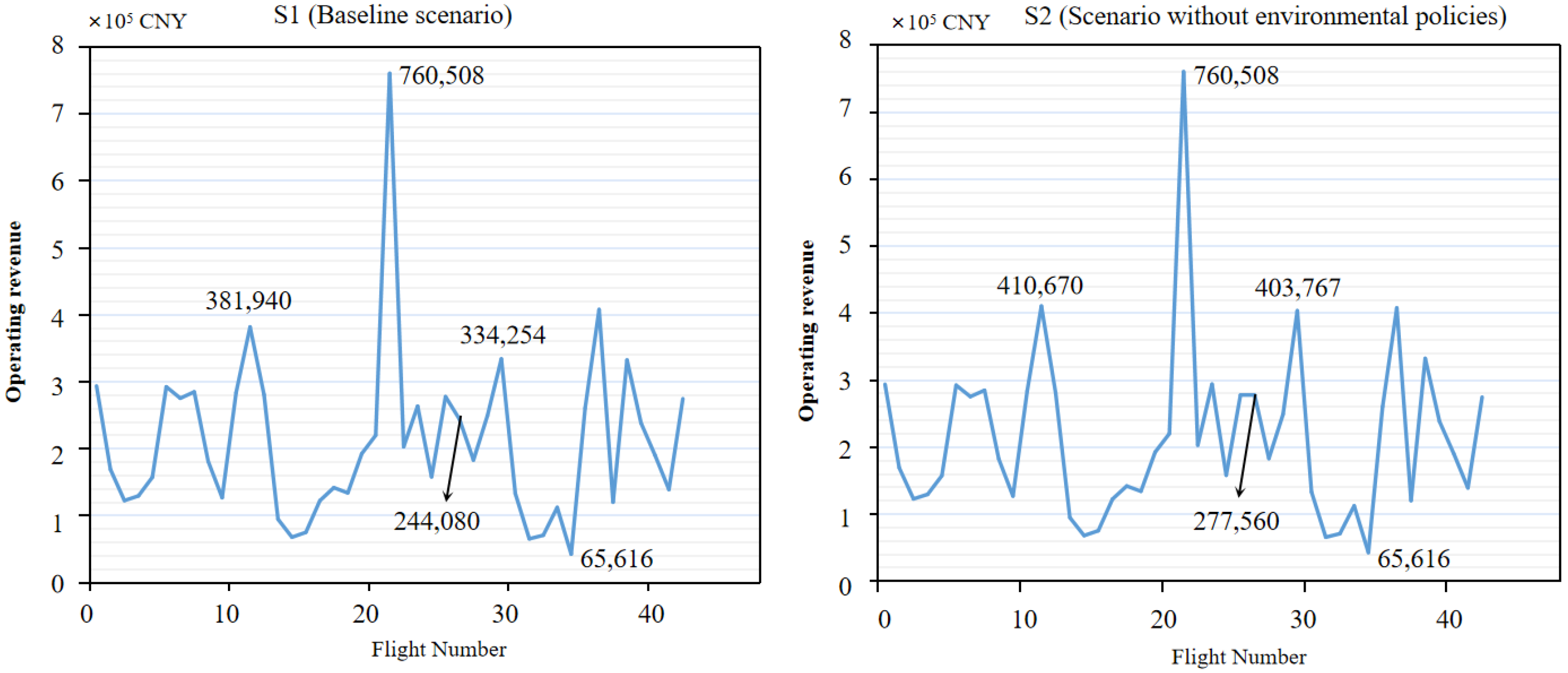
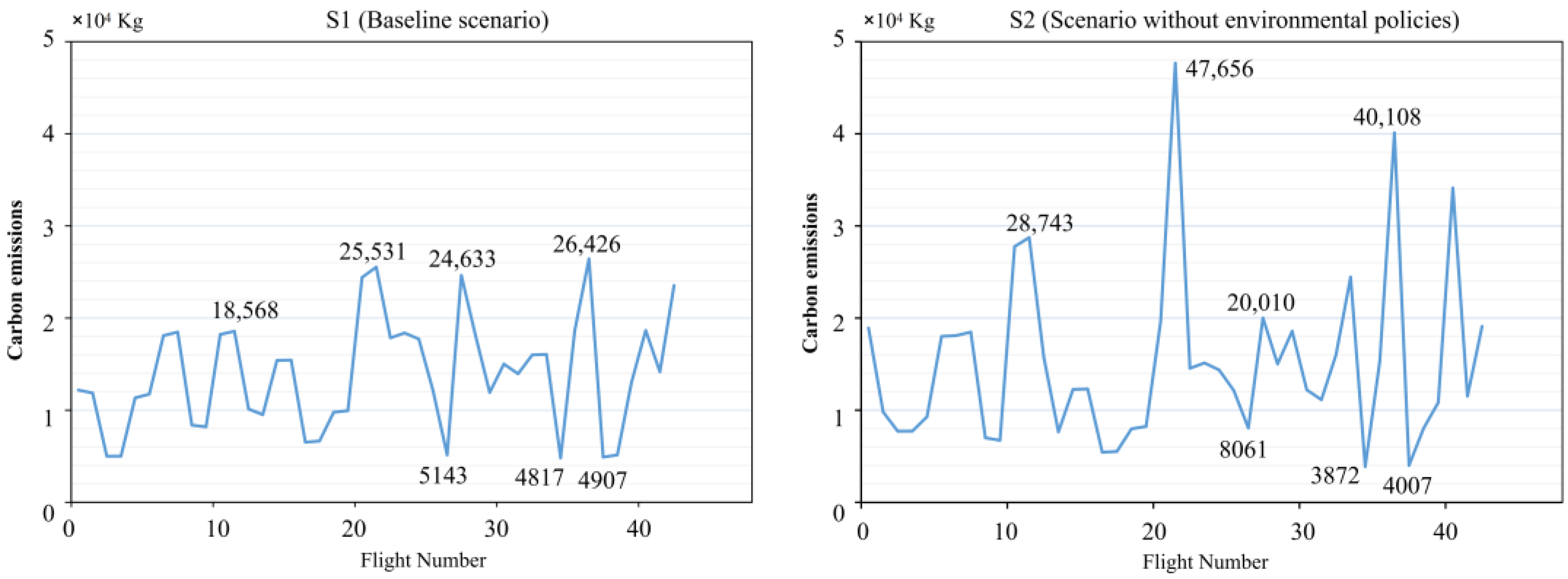
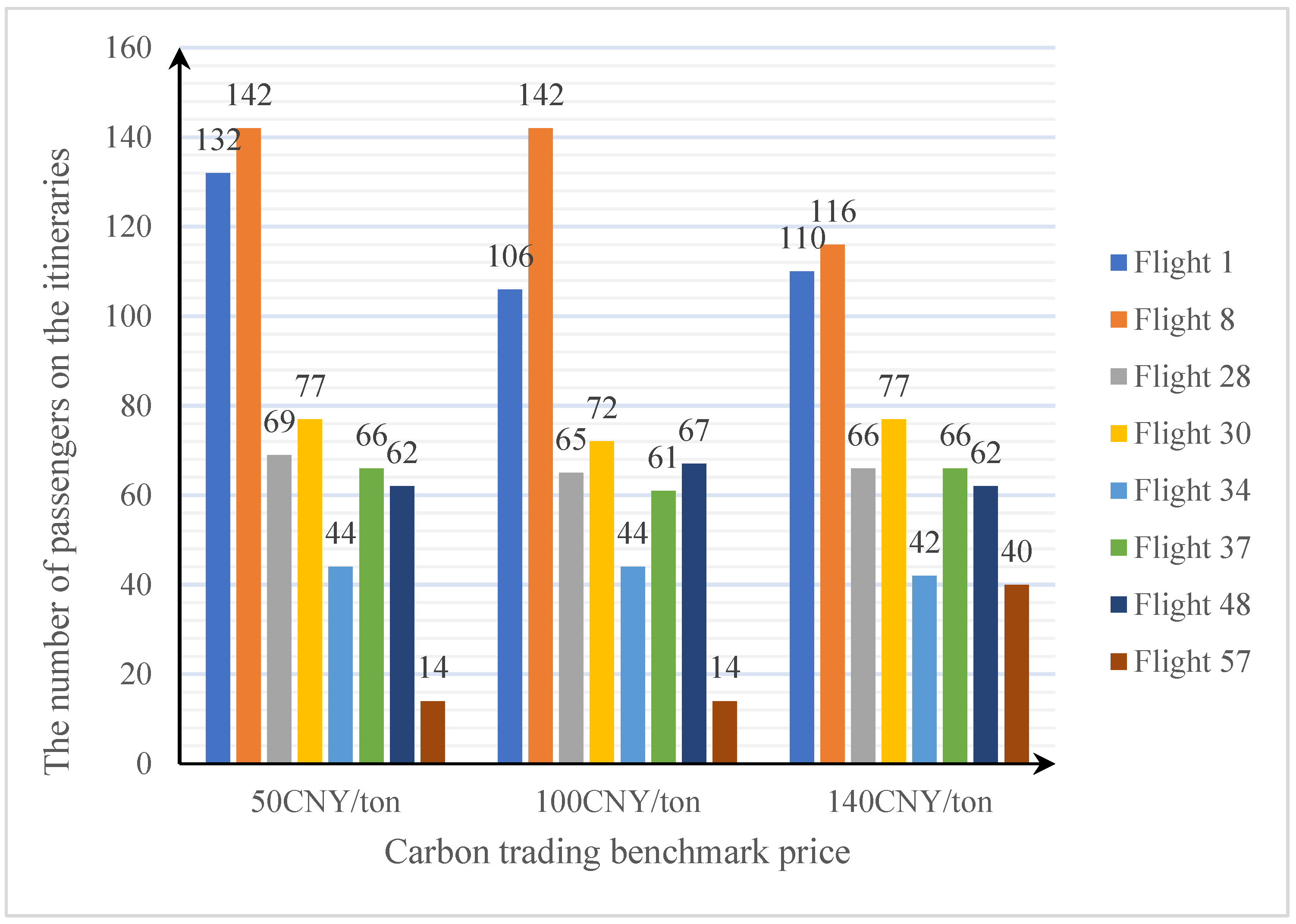
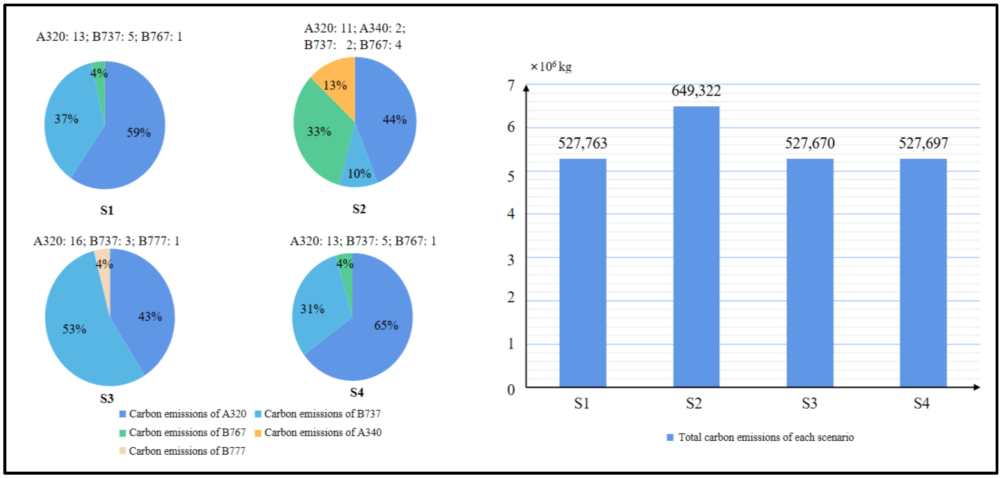
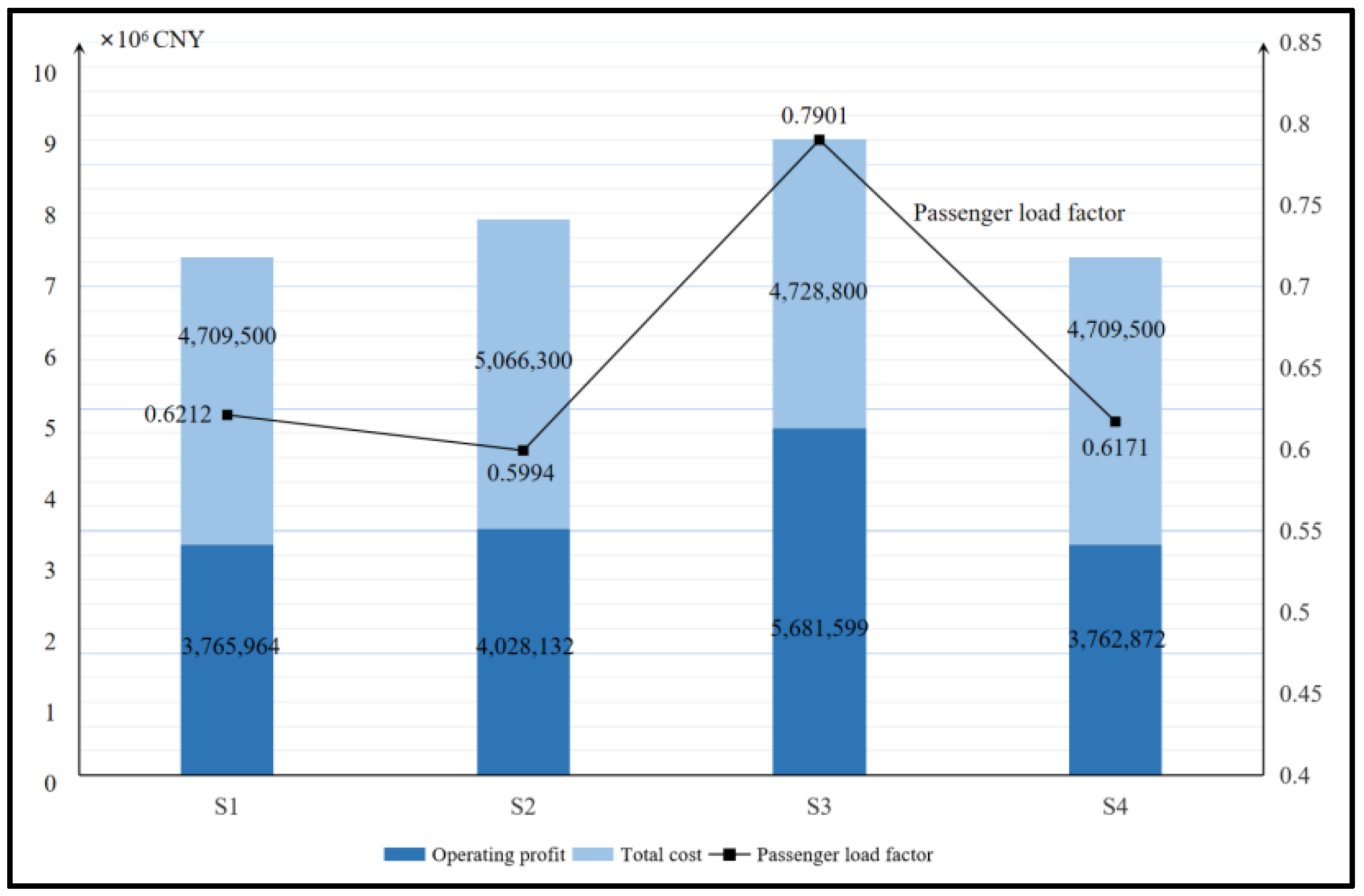
The comparison between S1 and S2 shows that the carbon emissions reduce by 23.03% when the profit only drops by 6.96% in a reasonable fleet. This suggests that the fleet planning method can reduce carbon emissions under the carbon trading mechanism with less effect on economic benefits. When the passenger demand level increases to 160%, airline profit increases by 50.86%, while carbon emissions almost remain the same. This verified that an optimized fleet is able to achieve the equilibrium of carbon reduction and economic performance under a higher passenger demand. Finally, the impact of carbon trading benchmark prices on the fleet is examined. The fleet optimized by this method is capable of coping with a higher carbon price by adjusting the number of passengers captured on each flight. According to the analyses of the above discussions, the insights are provided for stakeholders from the perspectives of governmental, industrial, and operational levels to achieve carbon neutrality.

Further research could be conducted in the following directions. Firstly, the current model only accounts for airlines’ predetermined flight schedules in a hub-and-spoke network, thus further extension to integrate fleet assignment and scheduling would be desirable. Secondly, as airlines may prioritize economic performance over carbon reduction measures due to their profitability, it would be valuable to explore how future societal and customer pressure could increase the reliability of green initiatives. In addition, exact approaches could be developed to solve the green fleet allocation problem on a larger route network.

References

1. Hd, A.; Jrb, C.; Jv, D.; Swa, E. Modeling deep decarbonization: Robust energy policy and climate action. Appl. Energy 2020, 262, 114517. [Google Scholar]
2. IEA (International Energy Agency). Global Energy Review: CO2 Emissions in 2021; IEA: Paris, France, 2022; Available online: https://www.iea.org/reports/global-energy-review-co2-emissions-in-2021-2 (accessed on 21 February 2023).
3. Sgouridis, S.; Bonnefoy, P.A.; Hansman, R.J. Air transportation in a carbon constrained world: Long-term dynamics of policies and strategies for mitigating the carbon footprint of commercial aviation. Transp. Res. Part A 2011, 45, 1077–1091. [Google Scholar] [CrossRef]
4. Terrenoire, E.; Hauglustaine, D.; Gasser, T.; Penanhoat, O. The contribution of carbon dioxide emissions from the aviation sector to future climate change. Environ. Res. Lett. 2019, 14, 084019. [Google Scholar] [CrossRef]
5. Chao, C.C. Assessment of carbon emission costs for air cargo transportation. Transp. Res. Part D Transp. Environ. 2014, 33, 186–195. [Google Scholar] [CrossRef]
6. Liu, Z.; Deng, Z.; He, G.; Wang, H.; Zhang, X.; Lin, J.; Qi, Y.; Liang, X. Challenges and opportunities for carbon neutrality in China. Nat. Rev. Earth Environ. 2022, 3, 141–155. [Google Scholar] [CrossRef]
7. TCFM (The Chinese Foreign Ministry). Statement by Xi Jinping President of the People’s Republic of China at the General Debate of the 75th Session of the United Nations General Assembly. 2020. Available online: https://www.fmprc.gov.cn/mfa_eng/zxxx_662805/t1817098.shtml (accessed on 17 June 2022).
8. Abdullah, M.A.; Chew, B.C.; Hamid, S.R. Benchmarking Key Success Factors for the Future Green Airline Industry. Procedia Soc. Behav. Sci. 2016, 224, 246–253. [Google Scholar] [CrossRef] [Green Version]
9. Migdadi, A.A. Identifying the effective taxonomies of airline green operations strategy. Manag. Environ. Qual. Int. J. 2019, 31, 146–166. [Google Scholar] [CrossRef]
10. Jalalian, M.; Gholami, S.; Ramezanian, R. Analyzing the trade-off between CO2 emissions and passenger service level in the airline industry: Mathematical modeling and constructive heuristic. J. Clean. Prod. 2019, 206, 251–266. [Google Scholar] [CrossRef]
11. Müller, C.; Kieckhäfer, K.; Spengler, T.S. The influence of emission thresholds and retrofit options on airline fleet planning: An optimization approach. Energy Policy 2018, 112, 242–257. [Google Scholar] [CrossRef]
12. Parsa, M.; Nookabadi, A.S.; Flapper, S.D.; Atan, Z. Green hub-and-spoke network design for aviation industry. J. Clean. Prod. 2019, 229, 1377–1396. [Google Scholar] [CrossRef]
13. Lozano, S.; Gutierrez, E. A multiobjective approach to fleet, fuel and operating cost efficiency of European airlines. Comput. Ind. Eng. 2011, 61, 473–481. [Google Scholar] [CrossRef]
14. Capaz, R.S.; Guida, E.; Seabra, J.E.; Osseweijer, P.; Posada, J.A. Mitigating carbon emissions through sustainable aviation fuels: Costs and potential. Biofuels Bioprod. Biorefining 2020, 15, 502–524. [Google Scholar] [CrossRef]
15. Csereklyei, Z.; Stern, D.I. Flying More Efficiently: Joint Impacts of Fuel Prices, Capital Costs and Fleet Size on Airline Fleet Fuel Economy. Ecol. Econ. 2020, 175, 106714. [Google Scholar] [CrossRef]
16. Oliveira, A.; Narcizo, R.R.; Caliari, T.; Morales, M.A.; Prado, R. Estimating fuel-efficiency while accounting for dynamic fleet management: Testing the effects of fuel price signals and fleet rollover. Transp. Res. Part D Transp. Environ. 2021, 95, 102820. [Google Scholar] [CrossRef]
17. Dray, L.; Evans, A.; Reynolds, T.; Schäfer, A.W.; Vera-Morales, M.; Bosbach, W. Airline fleet replacement funded by a carbon tax: An integrated assessment. Transp. Policy 2014, 34, 75–84. [Google Scholar] [CrossRef]
18. Khoo, H.L.; Teoh, L.E. A bi-objective dynamic programming approach for airline green fleet planning. Transp. Res. Part D 2014, 33, 166–185. [Google Scholar] [CrossRef]
19. Ma, Q.; Song, H.; Zhu, W. Low-carbon airline fleet assignment: A compromise approach. J. Air Transp. Manag. 2018, 68, 86–102. [Google Scholar] [CrossRef]
20. Wu, H.; Zeng, Y. Equilibrium investment strategy for defined-contribution pension schemes with generalized mean–variance criterion and mortality risk. Insur. Math. Econ. 2015, 64, 396–408. [Google Scholar] [CrossRef]
21. Qiu, R.; Xu, J.; Xie, H.; Zeng, Z.; Lv, C. Carbon tax incentive policy towards air passenger transport carbon emissions reduction. Transp. Res. Part D Transp. Environ. 2020, 85, 102441. [Google Scholar] [CrossRef]
22. Kang, J.H.; Wang, M.H.; Huang, N.J. Equilibrium strategy for mean–variance-utility portfolio selection under Heston’s SV model. J. Comput. Appl. Math. 2021, 392, 113490. [Google Scholar] [CrossRef]
23. Hu, X.; Yang, Z.; Sun, J.; Zhang, Y. Carbon Tax or Cap-and-Trade: Which is More Viable for Chinese Remanufacturing Industry? J. Clean. Prod. 2019, 243, 118606. [Google Scholar] [CrossRef] [Green Version]
24. Li, M.; Weng, Y.; Duan, M. Emissions, energy and economic impacts of linking China’s national ETS with the EU ETS. Appl. Energy 2019, 235, 1235–1244. [Google Scholar] [CrossRef]
25. Oesingmann, K. The effect of the European Emissions Trading System (EU ETS) on aviation demand: An empirical comparison with the impact of ticket taxes. Energy Policy 2022, 160, 112657. [Google Scholar] [CrossRef]
26. Liu, L.; Chen, C.; Zhao, Y.; Zhao, E. China’s carbon-emissions trading: Overview, challenges and future. Renew. Sustain. Energy Rev. 2015, 49, 254–266. [Google Scholar] [CrossRef]
27. Cao, J.; Ho, M.S.; Ma, R.; Teng, F. When carbon emission trading meets a regulated industry: Evidence from the electricity sector of China. J. Public Econ. 2021, 200, 104470. [Google Scholar] [CrossRef]
28. Cui, Q. Investigating the airlines emission reduction through carbon trading under CNG2020 strategy via a Network Weak Disposability DEA. Energy 2019, 180, 763–771. [Google Scholar] [CrossRef]
29. Lyu, J.; Cao, M.; Wu, K.; Li, H.; Mohi-ud-din, G. Price volatility in the carbon market in China. J. Clean. Prod. 2020, 255, 120171. [Google Scholar] [CrossRef]
30. Scheelhaase, J.; Maertens, S.; Grimme, W. Options for improving the EU Emissions Trading Scheme (EU ETS) for aviation. Transp. Res. Procedia 2021, 59, 193–202. [Google Scholar] [CrossRef]
31. Yin, K.S.; Dargusch, P.; Halog, A. An analysis of the greenhouse gas emissions profile of airlines flying the Australian international market. J. Air Transp. Manag. 2015, 47, 218–229. [Google Scholar] [CrossRef]
32. Zeng, B.; Xie, J.; Zhang, X.; Yu, Y.; Zhu, L. The impacts of emission trading scheme on China’s thermal power industry: A pre-evaluation from the micro level. J. Energy Environ. 2019, 31, 1007–1030. [Google Scholar] [CrossRef]
33. Xie, Z.T.; Liu, H.X. Stackelberg game based co-firing biomass with coal under carbon cap-and-trade regulation. J. Energy Environ. 2022, 33, 1369–1395. [Google Scholar] [CrossRef]
34. Repko, M.G.; Santos, B.F. Scenario tree airline fleet planning for demand uncertainty. J. Air Transp. Manag. 2017, 65, 198–208. [Google Scholar] [CrossRef] [Green Version]
35. Nabil Kenan, Aida Jebali, Ali Diabat, An integrated flight scheduling and fleet assignment problem under uncertainty. J. Comput. Oper. Res. 2018, 100, 333–342. [CrossRef]
36. Sa, C.A.; Santos, B.F.; Clarke, J.-P.B. Portfolio-based airline fleet planning under stochastic demand. J. Omega 2020, 97, 102101. [Google Scholar] [CrossRef]
37. Zuidberg, J. Identifying airline cost economies: An econometric analysis of the factors affecting aircraft operating costs. J. Air Transp. Manag. 2014, 40, 86–95. [Google Scholar] [CrossRef]
38. International Civil Aviation Organization (ICAO). Methodology ICAO Carbon Calculator V7; ICAO: Montreal, QC, Canada, 2014. [Google Scholar]
39. Cui, Q.; Li, X.Y.; Li, Y. Accounting for the carbon emissions from domestic air routes in China. Heliyon 2022, 8, e08716. [Google Scholar] [CrossRef]
40. Cui, Q. The online pricing strategy of low-cost carriers when carbon tax and competition are considered. Transp. Res. Part A Policy Pract. 2019, 121, 420–432. [Google Scholar] [CrossRef]
41. Hu, Z.; Yan, S.; Lv, C.; Yao, L. Sustainable development oriented bi-level dynamic programming method toward the coal–water conflict in China. J. Energy Environ. 2019, 30, 1396–1436. [Google Scholar] [CrossRef]
42. Liao, Z.; Zhu, X.; Shi, J. Case study on initial allocation of Shanghai carbon emission trading based on Shapley value. J. Clean. Prod. 2015, 103, 338–344. [Google Scholar] [CrossRef]
43. Xu, J.; Yang, X.; Tao, Z. A tripartite equilibrium for carbon emission allowance allocation in the power-supply industry. Energy Policy 2015, 82, 62–80. [Google Scholar] [CrossRef]
44. International Civil Aviation Organization (ICAO). ICAO Environmental Report 2013. Aviation and Climate Change. 2013. Available online: https://www.icao.int/environmental-protection/Documents/EnvironmentalReports/2013/ICAOEnvReport2013.pdf (accessed on 20 December 2021).
45. Markham, F.; Young, M.; Reis, A.; Higham, J. Does carbon pricing reduce air travel? Evidence from the Australian ‘Clean Energy Future’ policy, July 2012 to June 2014. J. Transp. Geogr. 2018, 70, 206–214. [Google Scholar] [CrossRef] [Green Version]
46. Ji, C.-J.; Hu, Y.-J.; Tang, B.-J.; Qu, S. Price drivers in the carbon emissions trading scheme: Evidence from Chinese emissions trading scheme pilots. J. Clean. Prod. 2021, 278, 123469. [Google Scholar] [CrossRef]
47. Mumbower, S.; Garrow, L.A.; Higgins, M.J. Estimating flight-level price elasticities using online airline data: A first step toward integrating pricing, demand, and revenue optimization. J. Transp. Res. Part A Policy Pract. 2014, 66, 196–212. [Google Scholar] [CrossRef]
48. Granados, N.; Gupta, A.; Kauffman, R.J. Online and offline demand and price elasticities: Evidence from the air travel industry. J. Inform. Syst. Res. 2012, 23, 164–181. [Google Scholar] [CrossRef] [Green Version]
49. Pagoni, I.; Psaraki-Kalouptsidi, V. The impact of carbon emission fees on passenger demand and air fares: A game theoretic approach. J. Air Transp. Manag. 2016, 55, 41–51. [Google Scholar] [CrossRef]
Figure 1. A concept model for the aviation carbon trading process.
Sustainability 15 05832 g001
Figure 2. Timeline without ground arc in Shijiazhuang airport.
Sustainability 15 05832 g002
Figure 3. Flight route map in hub-and-spoke network.
Sustainability 15 05832 g003
Figure 4. Flights on legs and itineraries through three airports.
Sustainability 15 05832 g004
Figure 5. Operating revenue of each itinerary for S1 and S2.
Sustainability 15 05832 g005
Figure 6. CO2 emissions on each flight for S1 and S2.
Sustainability 15 05832 g006
Figure 7. Comparison of the number of passengers between the scenarios in different carbon benchmark prices.
Sustainability 15 05832 g007
Figure 8. Left: carbon emissions of each aircraft type in four scenarios. Right: comparison of total carbon emissions in four scenarios.
Sustainability 15 05832 g008
Figure 9. Comparison of operating profit, total cost, and passenger load factor in four scenarios.
Sustainability 15 05832 g009