Mobile Phone Data Feature Denoising for Expressway Traffic State Estimation

Abstract

Due to their wide coverage, low acquisition cost and large data quantity, the mobile phone signaling data are suitable for fine-grained and large-scale estimation of traffic conditions. However, the relatively high level of data noise makes it difficult for the estimation to achieve sufficient accuracy. According to the characteristics of mobile phone data noise, this paper proposed an improved density peak clustering algorithm (DPCA) to filter data noise. In addition, on the basis of the long short-term memory model (LSTM), a traffic state estimation model based on mobile phone feature data was established with the use of denoising data to realize the estimation of the expressway traffic state with high precision, fine granules, and wide coverage. The Shanghai–Nanjing Expressway was used as a case study area for method and model verification, the results of which showed that the denoising method proposed in this paper can effectively filter data noise, reduce the impact of extreme noise data, significantly improve the estimation accuracy of the traffic state, and reflect the actual traffic situation in a fairly satisfactory manner.

1. Introduction

In recent years, China’s expressways have witnessed the increasingly wider application of smart systems. These smart expressway systems use various sensing equipment and traffic data detection equipment mainly for traffic information collection, integrated communication, intelligent computing, and control technologies to improve the safety, comfort, and efficiency of the transportation system, achieving the maximum utilization of road traffic resources.

A real-time and accurate estimation of the expressway traffic state is the prerequisite for the realization of the intelligent operation and control of a smart expressway system. For expressways, traffic flow speed is a key indicator reflecting road traffic states such as congestion. It is also one of the important indicators for traffic incident detection and identification. Therefore, the real-time and accurate estimation of the traffic flow speed is crucial to expressway intelligent control and operation.

It is often costly to install and maintain the current traffic data acquisition equipment, such as loop detectors, microwave detectors, and video detectors. A large amount of construction and maintenance resources are required to enable full coverage and fine-grained traffic flow estimation for accurate control. As smartphones are rapidly popularized in China, there have been many data sources that have emerged that are based on mobile communication devices, such as GPS data and mobile phone data. At present, they have become the important data sources required for traffic estimation and prediction.

Mobile communication service operators are responsible for generating mobile phone signaling data for communication and billing, which is advantageous in wide space coverage, low cost construction and maintenance, and larger data volume compared to the data collection by traditional traffic data acquisition equipment. However, mobile phone signaling data suffer a high data noise due to environmental factors and data acquisition methods. When high noise data are used to estimate the traffic state, the confidence coefficient and stability of the output results are insufficient for traffic state estimation, which cannot meet the requirements for practical application.

Therefore, it is essential to de-noise the data with the combined characteristics of mobile phone signaling data and their noise distribution. Based on the characteristics of mobile phone signaling data or mobile phone data, the noise can be filtered for estimating the traffic on expressway with fine particles, high precision, and wide coverage. This provides a crucial support for the intelligent control and operation of the expressway while improving the utilization rate of road resources.

2. Literature Review

Mobile phone signaling data are data generated from mobile phone communication [1]. These data are recorded through communication between mobile phones and cellular network base stations. Due to the temporal and spatial information contained in mobile phone signaling data, they are commonly employed to estimate and predict traffic and pedestrian flow. Basyoni [2] transformed cellular-network-based mobile phone data into vehicle-based data using data clustering algorithms without auxiliary systems, achieving good results for traffic flow estimation. Chen [3] investigated the feasibility of using mobile phone data for dynamic pedestrian flow prediction and reached an accuracy of over 75%. Caceres [4] inferred the number of vehicles moving between different region cells with anonymous call data from mobile phones as probes to estimate the traffic flow between regions. Janecek [5] estimated travel times and detected real-time road congestion on highways using anonymous mobile phone signaling data collected from mobile cellular networks. Huang [6] captured mobile flux in large-scale congestion events by combining mobile phone signaling data and city traffic data. Hillel [7] estimated traffic flow speed and travel time based on mobile phone signaling data from cellular phone service providers and compared the results with circular detectors, demonstrating an acceptable matching relationship between the two. Shen Li et al. [8] detected urban arterial traffic conditions with mobile phone data by the joint mutual information (JMI) feature selection method combined with the support vector machine method. Their experimental results suggested that the proposed method achieved a classification accuracy of 91% for low, medium, and high (three-level traffic states) traffic levels. Using feature extraction from raw mobile phone data and a three-level-long short-term memory model, Qiang Liu et al. [9] conducted large-scale field experiments on actual data collected during the 2014 “Golden Week” in Jiangsu Province, China. The proposed application performed well and became an emerging solution for traffic status monitoring with limited roadside sensing equipment.

However, the spatiotemporal uncertainty of mobile signaling data [10] results in high noise levels, became one of the main obstacles for large-scale application of such data. Currently, data cleaning typically involves removing short or incomplete trajectories containing only a small number of data points, interpolating missing data points (during long time intervals), and filtering outliers and noise considering their temporal and spatial features. Few studies describe data cleaning methods, and related research mainly focuses on filtering outliers and noise in the data. Li et al. [11] applied a rule-based method to overcome data oscillation. Kalatian and Shafahi [12] aggregated a group of cells near the fluctuations in the original data into a cell cluster and adopted the weighted center of the cells to replace them. Horn and Kern [13] and Horn et al. [14] removed anomalous data using the recursive forward-looking filter developed by Horn et al. [15]. These methods can handle some significantly incorrect or anomalous data, while further denoising mobile data or mobile data features is necessary during subsequent application stages in cases where high data quality is required.

Commonly used data noise identification and detection algorithms mainly include four types: classification-based algorithms [16,17], statistical-analysis-based algorithms [18,19], entropy-based algorithms [20], and clustering-based algorithms [21]. Clustering-based algorithms divide the data into categories following the similarity between the data points in the dataset and then determining some isolated points or categories, such as noise data, under certain criteria. With the division method, clustering algorithms can be further divided into partition-based data clustering algorithms, hierarchical clustering algorithms, model-based clustering algorithms, and density-based clustering algorithms. In this paper, an improved density peak clustering algorithm (DPCA) is proposed under the consideration of the characteristics of the uneven distribution of the original mobile speed feature samples and the characteristics of clustering methods to actively discover the clustering centers of data samples based on the difference in data point density and complete clustering. In this way, noise in mobile signaling data is further curtailed. Concurrently, a three-layer long short-term memory (LSTM) model is constructed with mobile data speed and quantity features, and feature data before and after denoising is employed to estimate the short-term traffic status of highways. LSTM is a powerful recursive neural system with excellent adaptability to time series and other related problems [22]. Experimental results reveal that the use of denoised feature data have higher estimation accuracy and stability.

3. Data Feature Extraction and Denoising

3.1. Data Preprocessing

Since the initial mobile signaling data collection contains a large amount of “dirty data”, such as duplicate data and missing fields, data preprocessing is necessary. Data preprocessing is composed of the following parts:

(1)

Processing of Mobile Identifiers

The processing of mobile identifiers simplifies and anonymizes the field that uniquely identifies mobile devices in the source data. This generates a unique digital code that distinguishes mobile data, contributing to saving storage space and assuring data security.

(2)

Processing of Invalid Data

Invalid data cannot be effectively used or involved in subsequent calculations. These types of data have problems such as missing data fields or abnormal field values and are processed through direct deletion.

(3)

Processing of Duplicate Data

In duplicate data, multiple rows have the same field values, or only the timestamp field has a short time interval difference, and the other fields have consistent values. For these types of data, only the first recorded data are retained, and the remaining records are discarded.

(4)

Processing of Ping-Pong Data

The ping-pong data that are generated are attributed to the overlapping coverage of base station signals in the communication network. As a result, the source of the signal received by the mobile device switches between multiple base stations, resulting in consecutive data records from the mobile device in which the communication area field switches repeatedly.

After deleting duplicate data, the data records of each mobile device are arranged in chronological order to identify the ping-pong data. Then, three consecutive data records are taken as a group. They are identified as ping-pong data if the base station information for these three data records switches back and forth between two base stations, and this happens more than twice with a switching time interval of less than the minimum time threshold. Only the first and last records of these types of data are retained, and the rest are deleted.

(5)

Processing of Drift Data

Drift indicates the situation where the base station communicating with the mobile phone changes to a farther one within a short period of time. In this case, the speed value of the mobile phone, calculated based on the drift data, is generally much larger than the normal value. Such data are not processed temporarily and will be further optimized in the subsequent analysis of mobile phone data characteristics.

3.2. Feature Extraction

The original mobile characteristic data used in this study consist of mobile speed data extracted from mobile signaling data. Mobile signaling data can generally be divided into two categories: switching data generated when the user makes or receives calls or messages; location update data generated by changes in the user’s location. As illustrated in the figure, the communication network records the switching information as mobile signaling data when a mobile phone switches between two adjacent communication cells. The location update data can be divided into three types in accordance with their source: location area data, determined by the phone when it is turned on and connected to the communication network; periodic location update data; and location update data, generated when a call is made across different areas. This study includes both types of data in the research scope as the original dataset to expand the original dataset. Subsequently, according to the method proposed by Ding et al. [23] for extracting mobile speed (PSP) and mobile count (PC), the center base station of each communication cell in the communication network is mapped to the highway with the projection point, and the accumulated mileage calculated with the route origin is assigned, allowing a single base station to obtain a unique mileage. Regarding each original data record containing only the base station identifier, the projection point of the corresponding base station is adopted to locate the phone and is represented as an erroneous record.

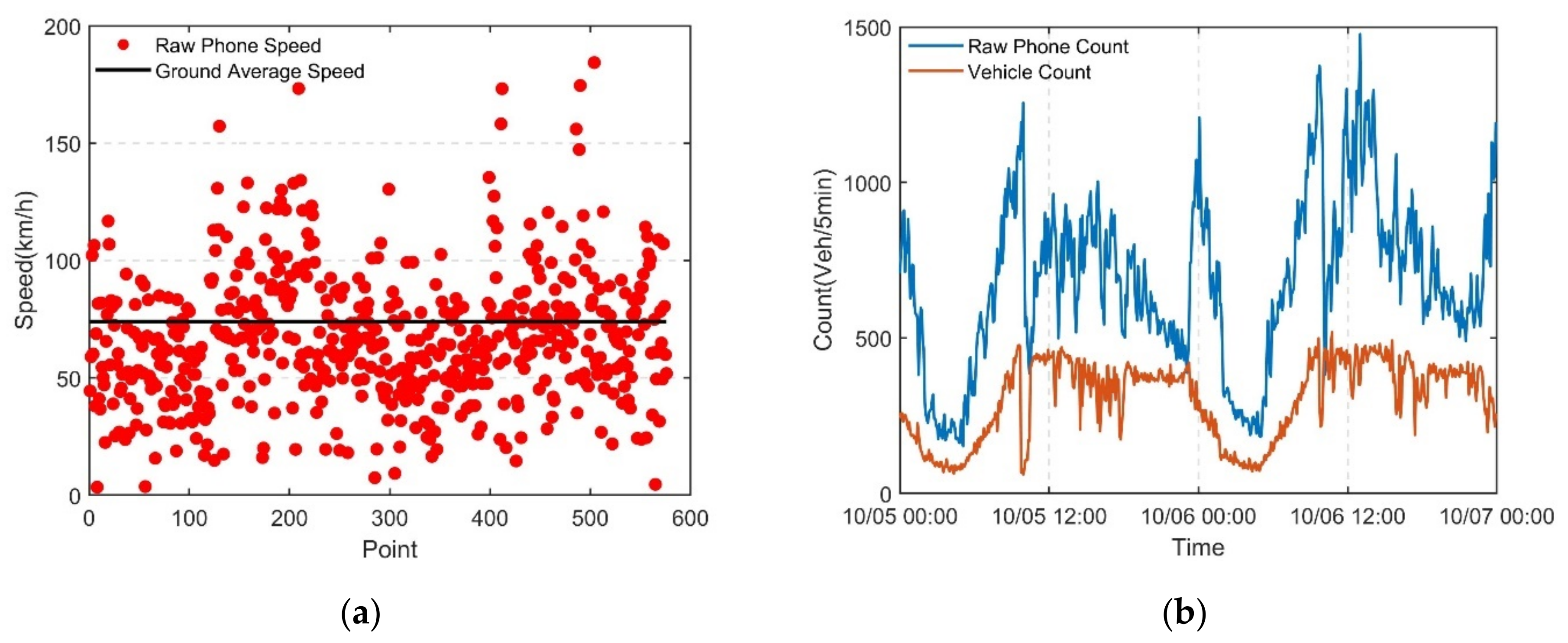
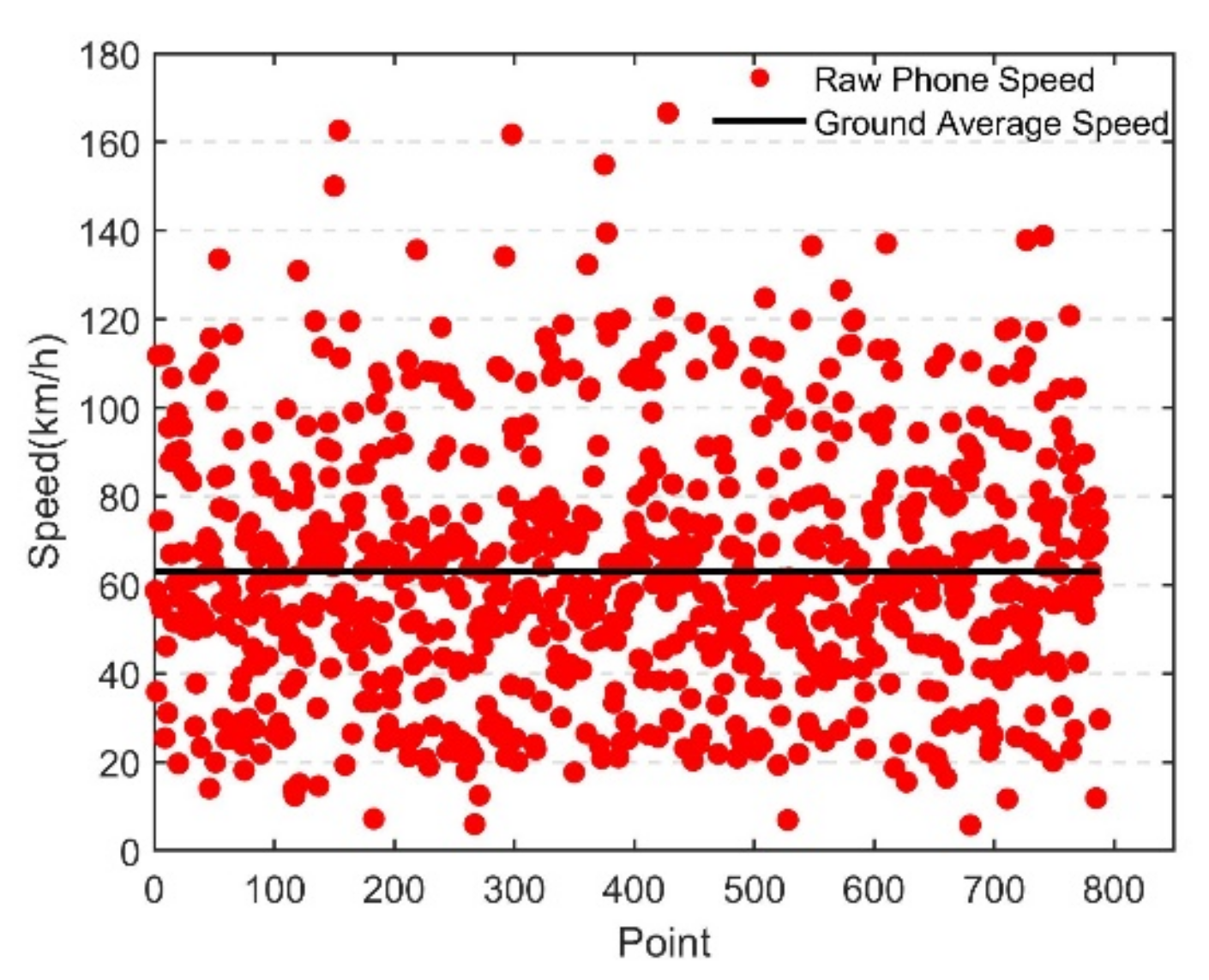
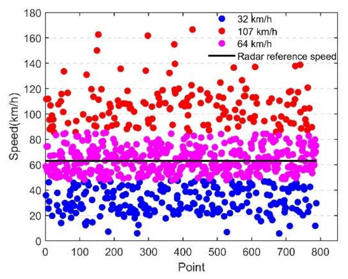
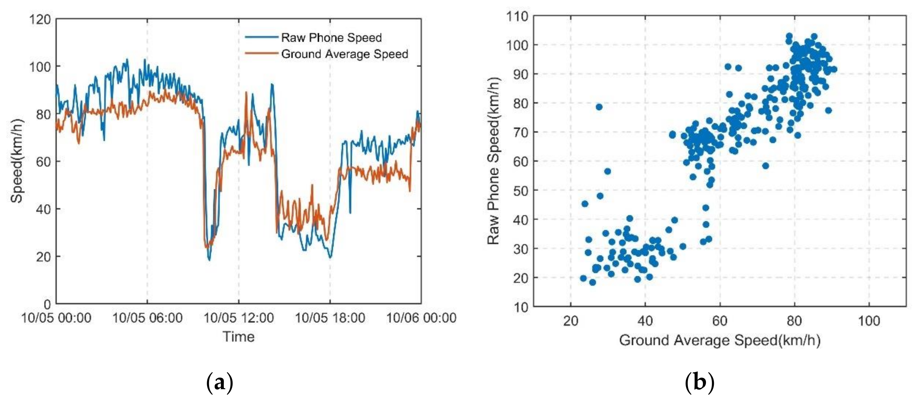
3.3. Origin of Data Noise

Figure 1 below shows the original speed feature dataset of mobile phones in a 5 min data slice extracted from the research data. The data points of mobile phone speed characteristics in the original dataset are widely distributed with the highest speed close to 180 km/h and the lowest speed close to 0 km/h, neither of which is the actual situation.

As shown in Figure 1b, the cross-sectional radar-measured traffic is compared with the corresponding original quantity eigenvalues of the mobile phones at a time interval of 5 min, and the latter is much greater than the former. Therefore, appropriate methods must be adopted for noise recognition and filtering to ensure the rationality and authenticity of the results of mobile phone speed eigenvalues and quantitative eigenvalues, as well as valid sample data for road traffic state estimation.

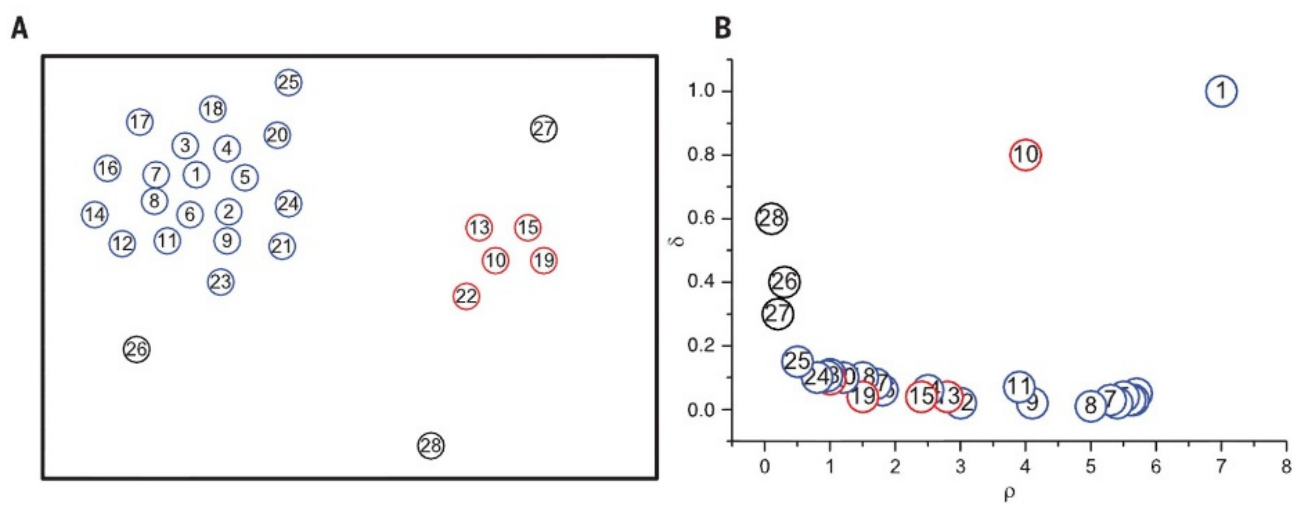
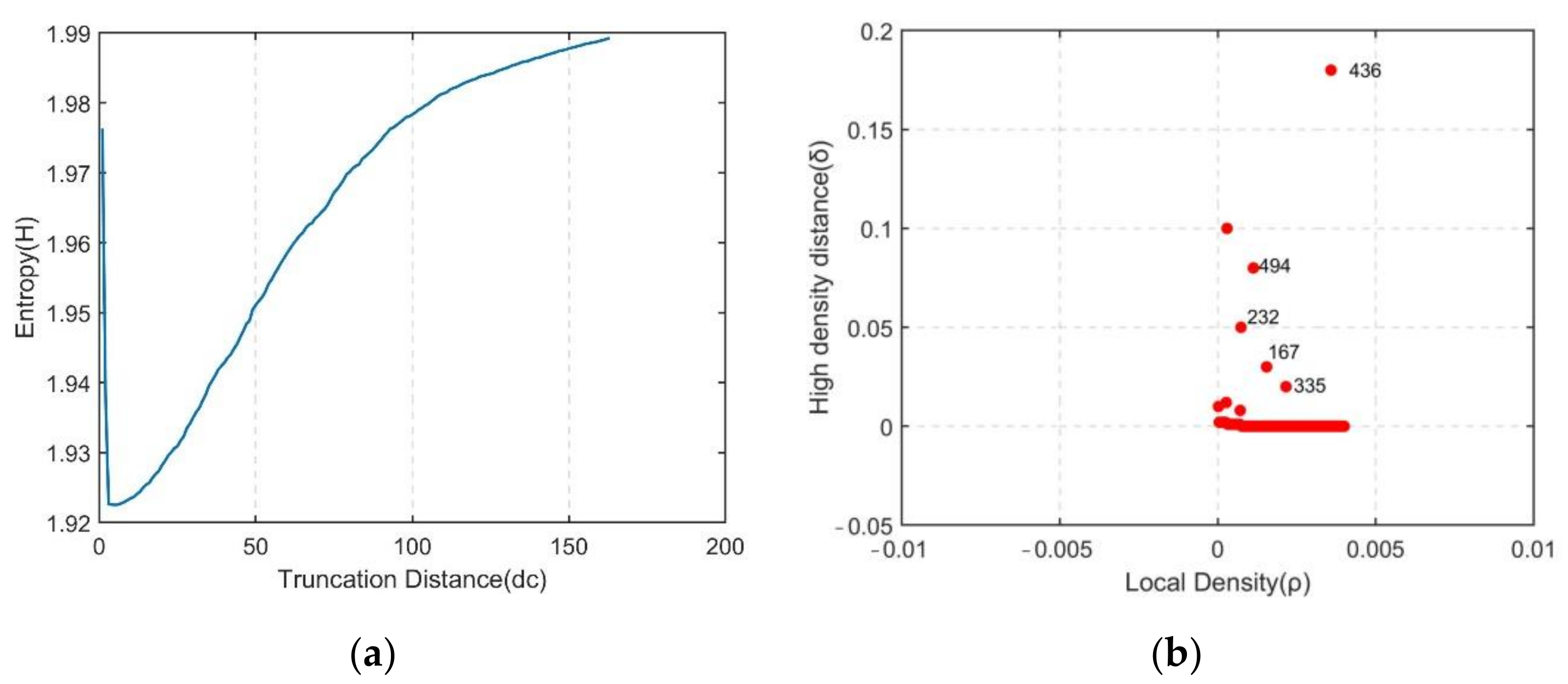
3.4. Feature Data Denoising Method Based on the Improved DPCA

The traditional DPCA generally assigns a value to the truncation distance parameter $d_c$ under subjective experience. This requires a deep understanding of the overall characteristics of the clustered data. Nonetheless, mobile signaling data in different clustering datasets have different distribution characteristics, and it is difficult to achieve satisfactory results by subjectively determining the truncation distance parameter.

Local density and high-density distance are used as measures when selecting cluster centers. With two-dimensional (2D) plane data points as an example, assume that there are N samples to be clustered. Then, concerning any data point $i$, the commonly used calculation method for its corresponding local density ${\delta }_i$ is

$${\rho }_i={{\displaystyle \sum }}_{j}exp\left(-{\left(\frac{d_{ij}}{d_c}\right)}^2\right),$$

(1)

The above formula is a calculation method for $d_c$ based on the Gaussian kernel, which can effectively avoid situations where different data points produce the same local density value. Another variable for calculating the high-density distance ${\delta }_i$ of the sample point is expressed as

$${\delta }_i=\underset{j:{\rho }_j>{\rho }_i}{\mathit{min}}\left(d_{ij}\right),$$

(2)

when the local density ${\rho }_i$ of sample point $i$ is the highest among all sample points, ${\delta }_i$ is defined as

$${\delta }_i=\underset{j}{\mathit{max}}\left(d_{ij}\right),$$

(3)

After the calculation of the local density and high-density distance for each sample, a 2D decision map is drawn with these two parameters. The points with both high local density and high-density distance can be determined as density peaks, which are the clustering centers.

Figure 2 exhibits a schematic of clustering center decisions based on the DPCA for 2D data. As observed in the figure, the original data are mainly distributed around two clustering centers, and there is a large gap between Sample Points 1 and 10, satisfying the two conditions mentioned above.

This method requires a comprehensive understanding of the overall characteristics of the clustered data. However, the mobile signaling data in different datasets that are to be clustered may have different distribution characteristics, and using subjective methods to determine the truncation distance parameter often fails to achieve satisfactory results.

Therefore, DPCA optimization based on mobile feature data denoising is proposed in this paper, described as:

(1)

Optimization of the adaptive selection of the cut-off distance ${\mathrm{d}}_{\mathrm{c}}$

The concept of “data field” is introduced. In a data field $\left(X=\left\{x\_1,x\_2,x\_3\dots x\_n\right\}\right)$ composed of several data points, for a data point $x_i$ in the field, the general field function of the data points in the data field is defined as follows:

$${\phi }_i={{\displaystyle \sum }}_j^n{e}^{-{\left(\frac{d_{ij}}{\sigma }\right)}^2},$$

(4)

In Equation (4), $\sigma$ is called radiation factor, and $d_{ij}$ is the distance between data point $x_i$ and data point $x_j$.

For a data field consisting of all data points, its potential entropy function is defined as follows:

$$H=-{{\displaystyle \sum }}_{i=1}^n\frac{{\phi }_i}{Z}\log \frac{{\phi }_i}{Z},$$

(5)

where $Z={\displaystyle \sum }_{i=1}^n{\phi }_i$ is called normalization factor.

According to the information theory, when the entropy of a system is large, the degree of chaos is high [24,25]. On the contrary, when the entropy is low, the overall system is less chaotic.

In DPCA, a point with higher local density is usually more likely to be a cluster center. Therefore, the optimal selection object can be transformed from the cut-off distance $d_c$ to the radiation factor $\sigma$, that is, seeking the minimum value of the potential entropy function, as shown in Equation (6):

$$\underset{\sigma }{\min }H=-{{\displaystyle \sum }}_{i=1}^n\frac{{\phi }_i}{Z}\log \frac{{\phi }_i}{Z},$$

(6)

(2)

Optimization of the cluster center automatic selection

In classic DPCA, two conditions to be satisfied by a clustering center have a relatively large local density, ${\rho }_i$ and high-density distance ${\gamma }_i$. Moreover, clustering center points are expected to have a large clustering center weight ${\gamma }_i$ [26], which boosts the likelihood of them being identified as clustering center points.

The main sources of noise for mobile data in the high-speed highway environment come from three categories: (1) The influence of adjacent parallel roads; (2) The influence of pedestrians’ mobile phone data; (3) The influence of network transmission errors. After calculating the clustering center weight γ of each data point, the data point with the maximum γ value is selected as the first actual clustering center, and the four points with γ values ranked 2–5 are selected as candidate clustering centers. Whether they are to be added as actual clustering centers is determined by the distance between the candidate clustering centers and the actual clustering center.

The distance between cluster centers is defined as the absolute difference in velocity values corresponding to the cluster center points. The final selected actual cluster centers must have distances between each other greater than the distance parameter $k_c$.

The classification standard of Chinese expressway traffic states shown in

Table 1. Chinese expressway traffic state classification standards.

Degree of Congestion	Design Speed (km/h)
	120	100	80
Free-flowing	[90, max)	[75, max)	[60, max)
Smooth	[60, 90)	[50, 75)	[40, 60)
Congested	[30, 60)	[25, 50)	[20, 40)
Severely congested	[0, 30)	[0, 25)	[0, 20)

implies that the speed range of the traffic state classification is mainly 20–30 km/h under different speed limit conditions. The value of the clustering center distance parameter $k_c$ is set as 20 km/h under the consideration of the short-term traffic state stability, the characteristics of mobile phone speed values, and the differences from actual vehicle speeds.

(3)

Optimization of valid data type selection

Figure 3 shows the clustering result of the selected original scatter sample data of mobile phone speed characteristics. The data points in the same colors belong to one class. According to the radar-measured speed, the pink data points in the figure are likely to reflect the valid data class of the actual traffic state during this period.

For the $i$th clustered data class, the overall density parameter $d_i$ and the quantity parameter $n_i$ of the data points in this class are calculated, respectively, as follows:

$$d_i=\frac{1}{D\times T_i}{{\displaystyle \sum }}_{t=1}^{T_i}{\rho }_t,$$

(7)

$$n_i=\frac{T_i}{N},$$

(8)

In Equations (7) and (8), $T_i$ is the total number of scattered data points in the $\mathrm{i}$th data class. $D={\displaystyle \sum }_{i=1}^c{a}_i$ is the normalization factor, where $c$ is the total number of clustered classes, $a_i$ is the average local density of data points in the $\mathrm{i}$th data class, and $N$ is the total number of data points in the entire dataset. The comprehensive scoring parameter $R$ is calculated by combining the above two parameters:

$$R_i=d_i\times n_i,$$

(9)

The class with the highest $R$ value is the valid data class that characterizes the current traffic state.

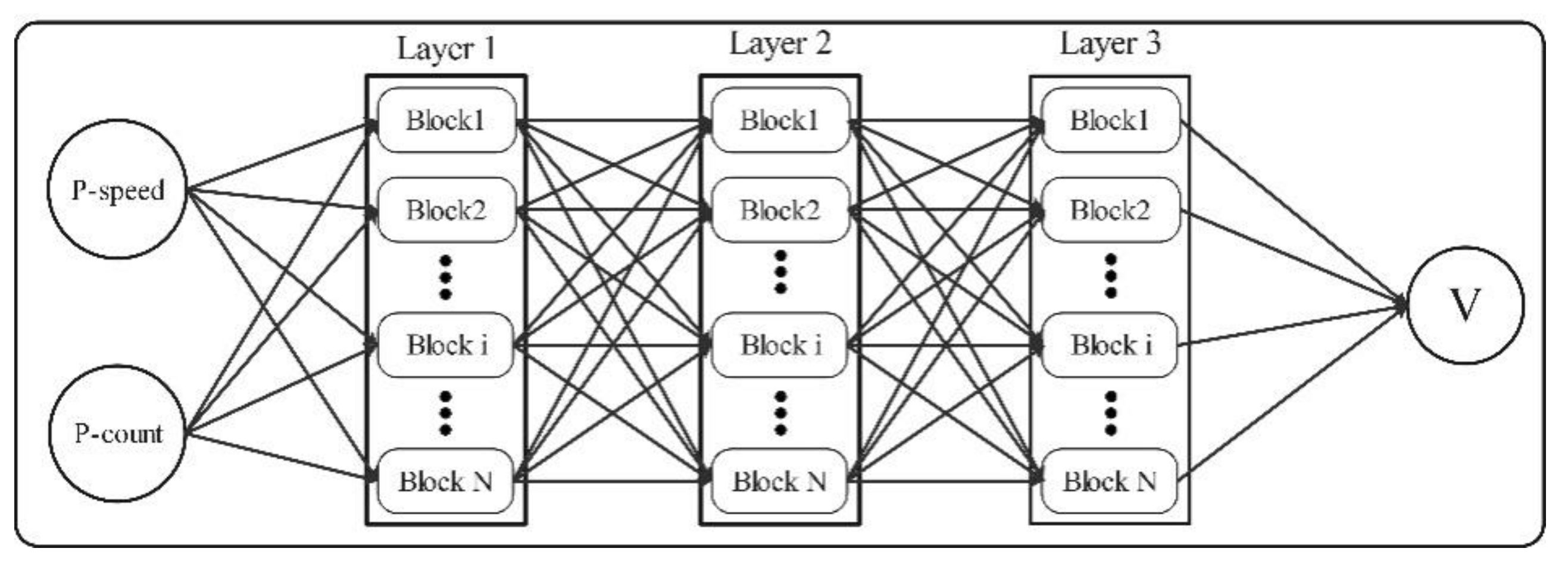
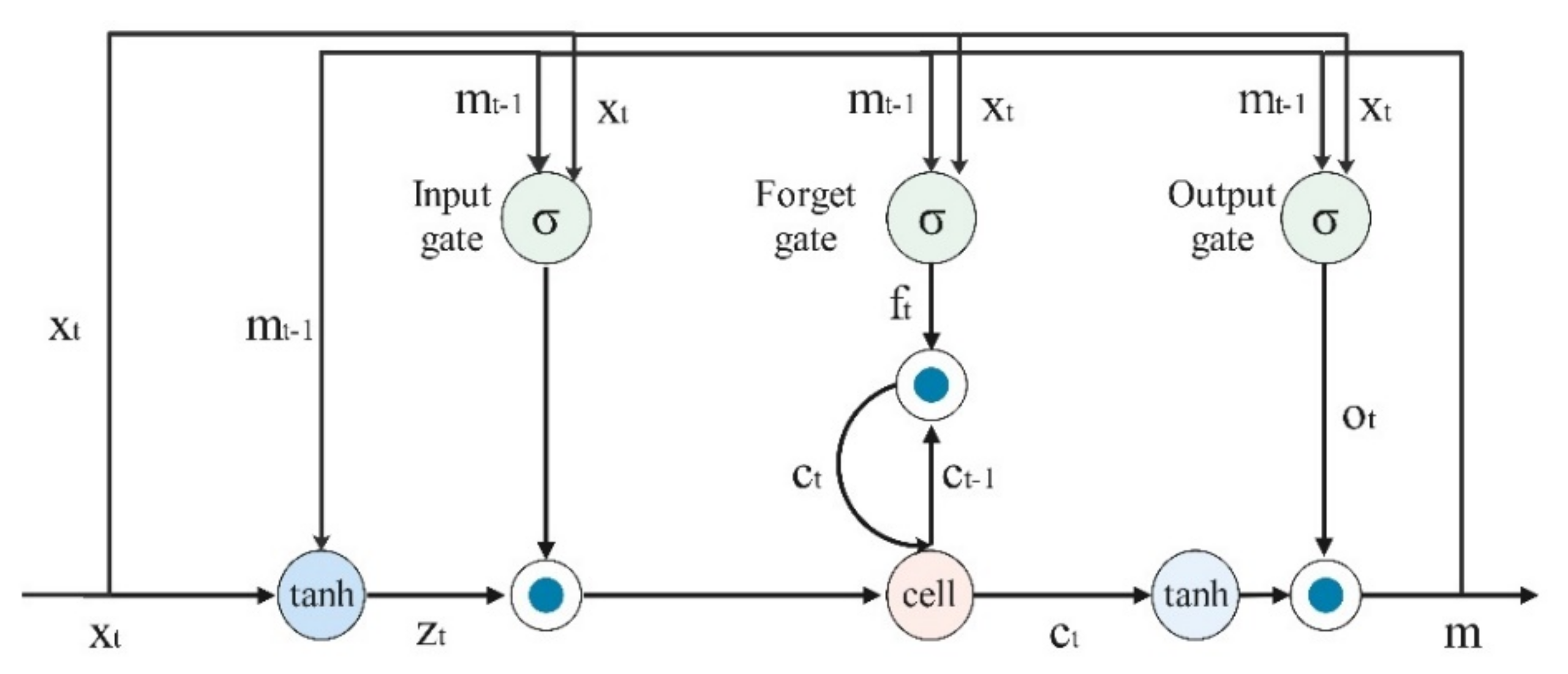
4. Construction of an LSTM-Based Traffic State Estimation Model

In contrast with the traditional multi-layer perceptron (MLP) model, the recurrent neural network (RNN) and LSTM model can better construct a model covering the contextual relevance of sequence data, achieving the fitting and modeling of the sequence data.

Considering the excellent performance of the deep learning model in related fields, such as pattern recognition, classification, estimation, and prediction, this paper established an LSTM network with three hidden layers to estimate the traffic flow speed of road sections, the basic structure of which is shown in Figure 4.

In Figure 4, P-speed represents the speed characteristic information of mobile phones, while P-count is the corresponding quantity characteristic information.

Each hidden layer in the model contains several memory units (block). The structure of a memory unit is shown in Figure 5. At time $t$, each memory unit calculates its gating structure and variable values based on the input variable $x_t$, hidden variable $m_{t-1}$, and memory cell state $c_{t-1}$.

The calculation process of each part in the $\mathrm{k}$th hidden layer is as follows:

The input gate ${\mathrm{i}}_{\mathrm{t}}^{\mathrm{k}}$ is calculated as follows:

$$i_t^k=sigmoid\left(W_{i,x}^k{x}_t^k+W_{i,m}^k{m}_{t-1}^k+b_i^k\right),$$

(10)

The forget gate ${\mathrm{f}}_{\mathrm{t}}^{\mathrm{k}}$ is calculated as follows:

$$f_t^k=sigmoid\left(W_{f,x}^k{x}_t^k+W_{f,m}^k{m}_{t-1}^k+b_f^k\right),$$

(11)

The output gate ${\mathrm{o}}_{\mathrm{t}}^{\mathrm{k}}$ is calculated as follows:

$$o_t^k=sigmoid\left(W_{o,x}^k{x}_t^k+W_{o,m}^k{m}_{t-1}^k+b_o^k\right),$$

(12)

The intermediate state ${\mathrm{z}}_{\mathrm{t}}^{\mathrm{k}}$ is calculated as follows:

$$z_t^k=tanh\left(W_{z,x}^k{x}_t^k+W_{z,m}^k{m}_{t-1}^k+b_z^k\right),$$

(13)

The memory cell state ${\mathrm{c}}_{\mathrm{t}}^{\mathrm{k}}$ is calculated as follows:

$$c_t^k=f_t^k\odot c_{t-1}^k+i_t^k\odot z_t^k,$$

(14)

The output state ${\mathrm{m}}_{\mathrm{t}}^{\mathrm{k}}$ is calculated as follows:

$$m_t^k=o_t^k\odot tanh\left(c_t^k\right),$$

(15)

The input data of the model used in this paper are the data sequences of mobile phone speed eigenvalues and quantity eigenvalues, which are relevant to directions and road sections, within a time interval of 5 min. This ensures that the model can better “learn” the correlation characteristics of the data in the time dimension during model training and verification. The final output of the model is an estimate of the traffic flow speed based on the target time interval, road section, and travel direction.

5. Case Study

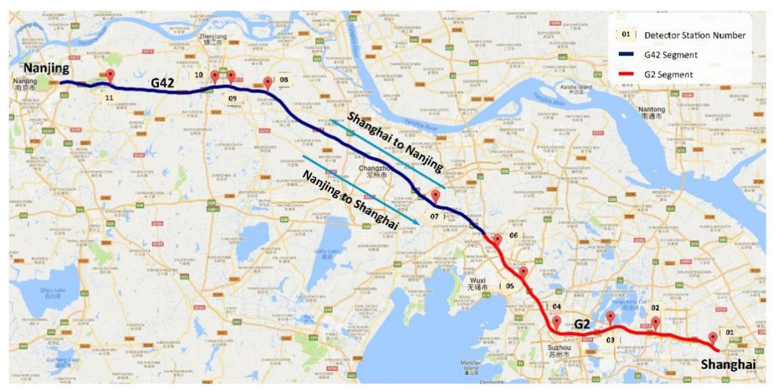
5.1. Source Data

The original speed feature data of mobile phones and the radar-measured data used in the case study of this paper were collected from the main sections of the Shanghai–Nanjing Expressway, as shown in Figure 6. The Shanghai–Nanjing Expressway is a section of the G42 Shanghai–Chengdu Expressway, and the first expressway constructed in the Jiangsu Province. On the map below, where the No. 1 microwave radar detector is located, is marked as section 1. The same rule applies to all the remaining sections.

The above-mentioned target road was divided into more than 220 road sections with each having a length of about 1–2 km. With the data feature extraction method described above, the direction-based and time-interval-based original speed feature sample datasets of mobile phones for each road section were obtained.

In this study, raw mobile phone data from 5 to 6 October 2015 were collected in the Nanjing–Shanghai direction. The data were collected at five-minute intervals and generated a total of 576 data slices, with a maximum number of mobile phones in a single pre-processed data slice of 1477, and a minimum of 152. Additionally, radar data from the same time period were used as a comparative validation dataset. Considering the possibility of missing data in the radar data, the Lagrange interpolation method was employed to maintain consistency in the spatiotemporal features between the two datasets.

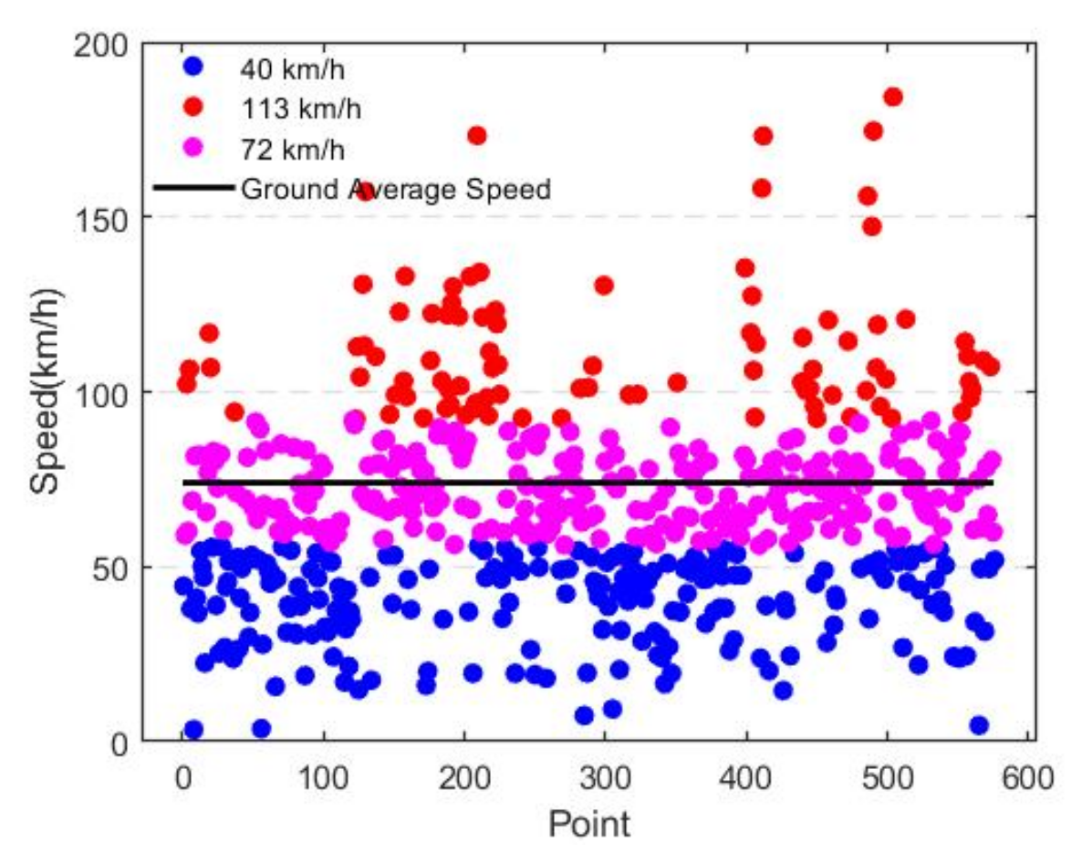
5.2. Mobile Phone Feature Data Denoising Based on the Improved DPCA

The original speed feature dataset of mobile phones extracted from 12:00 a.m. to 12:05 a.m. on 5 October 2015, on the No. 6 section of the Shanghai–Nanjing Expressway in the Nanjing–Shanghai direction is used as an example, and the distribution of data points is shown in Figure 7.

The correlation between the truncation distance $d_c$ and the overall entropy of the corresponding “data field” obtained through denoising calculations is illustrated in Figure 8. This figure demonstrates that as the truncation distance increases, the system entropy value of the “data field” exhibits a trend of first decreasing and then increasing. In other words, the system entropy value has a minimum value. Specifically, the truncation distance corresponding to the minimum entropy value is the optimal truncation distance $d_c$ following the scatter plot distribution characteristics of the dataset. The optimal truncation distance obtained through this scatter dataset is 5.14.

The local density ρ and high-density distance δ of each data point is calculated with the optimal truncation distance. Furthermore, the clustering center weights γ are computed. The resulting 2D decision graph is presented in Figure 8b. It can be observed from the figure that data point 436 has both a high local density and a high-density distance.

With respect to the change in clustering center weights, the top five data points in terms of clustering center weights are 436, 494, 232, 167, and 335, corresponding to speed feature values of 64 km/h, 32 km/h, 60 km/h, 26 km/h, and 107 km/h, respectively. The clustering center selection principle proposed in this paper reflects that the distance between each center point should be greater than the predetermined distance parameter. Therefore, the final clustering center selection consists of three data points with the identifiers 436, 494, and 335.

The clustering results are rendered in Figure 9, where the red, pink, and blue data points denote the clusters formed by data points with speed values of 107 km/h, 64 km/h, and 32 km/h, respectively. The speed values of the data points in the cluster formed by the data point with a speed value of 64 km/h are closest to the radar reference speed value, suggesting a high probability of being valid data points.

After a comprehensive evaluation of Score R of the above data clusters was performed, the speed value of the clustering center was determined to be 64 km/h. The resulting speed feature value for this data slice was 64, and the mobile device feature value was 362.

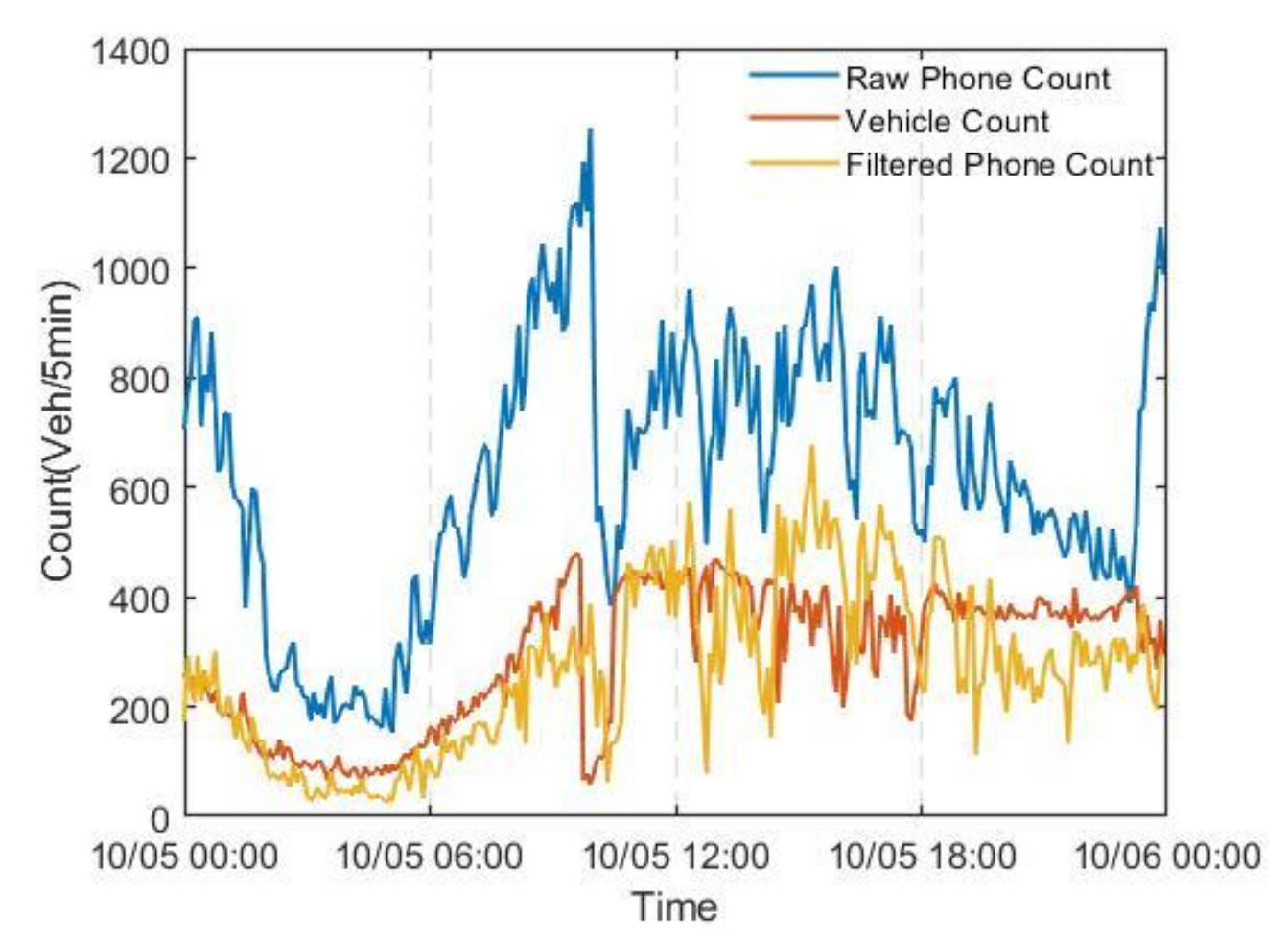
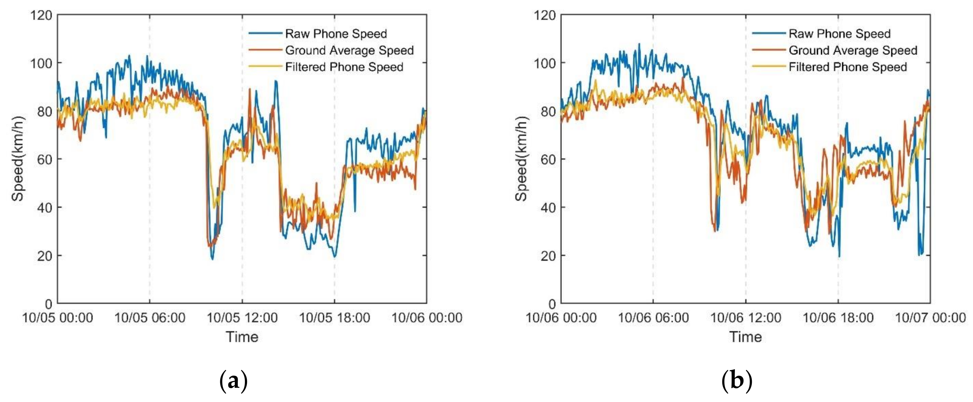
Denoising Effect Analysis

Figure 10 and Figure 11 compare the speed feature values of mobile phones before and after denoising with the measured radar speed, respectively.

The analysis of the speed scatter plot reveals that in the low-speed section with the radar speed of 20 km/h to 45 km/h and the high-speed section with the radar speed of 70 km/h to 90 km/h, the denoised speed feature values of mobile phones corresponding to the same radar speed fluctuate within a smaller range. In addition, in the scatter mapping plot after denoising, the scatter points are more likely to be distributed along either side of the 45-degree straight line, which is also more beneficial to the subsequent parameter learning of neural network models.

Figure 12 compares the quantity feature values of mobile phones before and after denoising with the corresponding radar-measured traffic, respectively.

The calculation demonstrates that the mean ratio of the mobile quantity feature value to the corresponding measured radar flow decreased from 2.78 before denoising to 0.95, and the variance of the ratio decreased from 3.32 to 0.36. After denoising, the ratio between the mobile quantity feature value and the corresponding flow was closer to 1.

5.3. Traffic State Estimation Based on Denoising Data

This section makes a further estimation of the traffic flow speed of the road sections using the LSTM model according to the mobile phone speed eigenvalues and quantity eigenvalues obtained based on the denoising data.

Accuracy Evaluation of the Traffic State Estimation Model

Figure 13 shows the traffic flow speed estimation results obtained from section 6 of the Shanghai–Nanjing Expressway in the Nanjing–Shanghai direction on 5 and 6 October 2015 based on the mobile phone feature data and the traffic state estimation model. The estimation accuracy is more intuitive and significantly improved after denoising.

Table 2. Comparison of quantitative indicators of traffic state estimation models.

Evaluation Index	Design Speed (km/h)
	5 October 2015		6 October 2015
	Raw Data	Filtered Data	Raw Data	Filtered Data
MSE (km2/h2)	134.41	57.34	268.61	87.59
MAE (km/h)	9.73	4.98	13.01	6.32
ME (km/h)	−5.16	−1.61	−4.78	−0.52
MAPE (%)	17.37	10.71	21.32	11.32

demonstrates the quantitative index analysis of the two types of data from the perspectives of mean square error (MSE), mean absolute error (MAE), mean error (ME), and mean absolute percentage error (MAPE). It indicates that the model that was trained with and applied the filtered feature data of mobile phones shows higher estimation accuracy of traffic flow speed than that based on the original mobile phone feature data. Moreover, the former model presents a smaller mean square error value than its counterpart, less than 2 km/h average error between the radar-measured value, and no more than 12% average error percentage (MAPE).

Furthermore, the Gaussian process and k-means clustering methods are introduced to denoise the mobile phone characteristic data, for comparison with the proposed method of denoising mobile phone data characteristics based on improved DPCA. The results are shown in

Table 3. Comparison in the quantitative indicators of traffic estimation between different denoising methods.

Evaluation Index	Design Speed (km/h)
	5 October 2015			6 October 2015
	Gaussian	k-Means	The Improved DPCA	Gaussian	k-Means	The Improved DPCA
MSE (km2/h2)	100.60	85.67	57.34	196.80	219.18	87.59
MAE (km/h)	8.72	7.57	4.98	12.08	11.13	6.32
ME (km/h)	−5.18	−2.16	−1.61	−4.85	−1.78	−0.52
MAPE (%)	15.95	14.47	10.71	19.39	18.26	11.32

. According to the comparison between the mean square error (MSE), mean error (ME), mean absolute value error (MAE), and mean absolute percentage error (MAPE) in the table, it can be concluded that the various indicators of accuracy of traffic flow speed estimation as achieved by the model training of the mobile phone characteristic data filtered through the improved DPCA denoising method are more effective.

To conclude, the traffic state estimation method with feature denoising data of mobile phones proposed in this paper can effectively remove the noise from the original mobile phone data characteristics, thereby reducing the influence of extreme values in the original data and improving the estimation accuracy and stability of traffic flow speed.

6. Summary

In this study, the characteristics of effective and noisy data in the context of data were explored, and an improved density peak clustering algorithm was designed to filter noise from raw mobile speed feature data. Moreover, a traffic state estimation model based on LSTM is established for highway traffic state estimation following the time-correlated features of the mobile speed feature data sequence. The effectiveness of the proposed data denoising method was verified using the raw mobile speed feature data and radar-measured data collected during the 2015 National Day on the Shanghai–Nanjing Expressway. The results demonstrated that the denoising method presented in this study effectively filtered data noise, weakened the impact of extreme noise data, significantly improved the estimation accuracy of the model, and reflected the details and actual traffic situations of highway traffic states, with good application prospects.

Although the system-entropy-value-based approach proposed in this study for selecting the optimal truncation distance parameter is more scientifically reliable than the subjective determination of the truncation distance parameter, it may still miss the optimal value, and thus, impact the clustering effect. Therefore, further optimization is needed to investigate the production mode of the set of alternative truncation distances in the future. Meanwhile, the time-correlation characteristics between the mobile speed features before and after this period were neglected when effective data were selected by constructing rating parameters. In the future, the spatiotemporal correlation characteristics of traffic flow should be considered in further exploring the selection of effective data to make the selection of effective data more scientifically reasonable.

Compared to the traditional methods of traffic state data collection, mobile signaling data have the advantages of low acquisition cost and wide coverage, which can achieve broad spatial coverage and comprehensive monitoring of highway traffic states. With the continuous improvement of traffic state estimation methods based on mobile signaling data and the increase in result confidence, the solution for traffic detection based on mobile signaling data has a promising future.

References

- Rose, G. Mobile phones as traffic probes: Practices, prospects and issues. Transp. Rev. 2006, 26, 275–291. [Google Scholar] [CrossRef]
- Yarah, B. Travel speed estimation from cellular networks using modified Data Swarm Clustering algorithm. In Proceedings of the ICET 2014-2nd International Conference on Engineering and Technology, Coimbatore, India, 8 July 2014. [Google Scholar]
- Chen, X.; Wan, X.; Ding, F.; Li, Q.; McCarthy, C.; Cheng, Y.; Ran, B. Data-Driven Prediction System of Dynamic People-Flow in Large Urban Network Using Cellular Probe Data. J. Adv. Transp. 2019, 2019, 9401630. [Google Scholar]
- Caceres, N.; Romero, L.M.; Benitez, F.G.; del Castillo, J.M. Traffic Flow Estimation Models Using Cellular Phone Data. IEEE Trans. Intell. Transp. Syst. 2012, 13, 1430–1441. [Google Scholar] [CrossRef]
- Janecek, A.; Valerio, D.; Hummel, K.A.; Ricciato, F.; Hlavacs, H. The Cellular Network as a Sensor: From Mobile Phone Data to Real-Time Road Traffic Monitoring. IEEE Trans. Intell. Transp. Syst. 2015, 16, 2551–2572. [Google Scholar] [CrossRef]
- Huang, Z.; Ling, X.; Wang, P.; Zhang, F.; Mao, Y.; Lin, T.; Wang, F.Y. Modeling real-time human mobility based on mobile phone and transportation data fusion. Transp. Res. Part C Emerg. Technol. 2018, 96, 251–269. [Google Scholar] [CrossRef]
- Hillel, B. Evaluation of a cellular phone-based system for measurements of traffic speeds and travel times: A case study from Israel. Transp. Res. Part C Emerg. Technol. 2007, 15, 380–391. [Google Scholar]
- Li, S.; Li, G.; Cheng, Y.; Ran, B. Urban arterial traffic status detection using cellular data without cellphone GPS information-ScienceDirect. Transp. Res. Part C Emerg. Technol. 2020, 114, 446–462. [Google Scholar] [CrossRef]
- Liu, Q.; Xie, J.; Ding, F. A Data-Driven Feature Based Learning Application to Detect Freeway Segment Traffic Status Using Mobile Phone Data. Sustainability 2021, 13, 7131. [Google Scholar] [CrossRef]
- Wang, F.; Chen, C. On data processing required to derive mobility patterns from passively-generated mobile phone data. Transp. Res. Part C Emerg. Technol. 2018, 87, 58–74. [Google Scholar] [CrossRef] [PubMed]
- Li, G.; Chen, C.-J.; Peng, W.-C.; Yi, C.-W. Estimating crowd flow and crowd density from cellular data for mass rapid transit. In Proceedings of the 6th International Workshop on Urban Computing, Halifax, NS, Canada, 14–17 August 2017. [Google Scholar]
- Kalatian, A.; Shafahi, Y.; Figueira, M. Travel Mode Detection Exploiting Cellular Network Data. MATEC Web Conf. 2016, 81, 03008. [Google Scholar] [CrossRef] [Green Version]
- Horn, C.; Kern, R. Deriving Public Transportation Timetables with Large-Scale Cell Phone Data. Procedia Comput. Sci. 2015, 52, 67–74. [Google Scholar] [CrossRef] [Green Version]
- Horn, C.; Gursch, H.; Kern, R.; Cik, M. QZTool-Automatically Generated Origin-Destination Matrices from Cell Phone Trajectories. Adv. Hum. Asp. Transp. 2017, 484, 823–833. [Google Scholar]
- Horn, C.; Klampfl, S.; Cik, M.; Reiter, T. Detecting Outliers in Cell Phone Data: Correcting Trajectories to Improve Traffic Modeling. Transp. Res. Rec. 2014, 2405, 49–56. [Google Scholar] [CrossRef] [Green Version]
- Grubbs, F.E. Procedures for detecting outlying observations in samples. Technometrics 1969, 11, 1–21. [Google Scholar] [CrossRef]
- Lv, F.; Liang, T.; Zhao, J.; Zhuo, Z.; Wu, J.; Yang, G. Latent Gaussian process for anomaly detection in categorical data. Knowl.-Based Syst. 2021, 220, 106896. [Google Scholar] [CrossRef]
- Zhang, A.; Song, S.; Wang, J. Sequential Data Cleaning: A Statistical Approach. In Proceedings of the 2016 International Conference on Management of Data, San Francisco, CA, USA, 26 June–1 July 2016. [Google Scholar]
- Fang, C.; Wang, F.; Yao, B.; Xu, J. GPSClean: A Framework for Cleaning and Repairing GPS Data. ACM Trans. Intell. Syst. Technol. 2022, 13, 1–22. [Google Scholar] [CrossRef]
- Desforges, M.J.; Jacob, P.J.; Cooper, J.E. Applications of probability density estimation to the detection of abnormal conditions in engineering. Proc. Inst. Mech. Eng. Part C J. Mech. Eng. Sci. 1998, 212, 687–703. [Google Scholar] [CrossRef]
- Song, S.; Li, C.; Zhang, X. Turn Waste into Wealth: On Simultaneous Clustering and Cleaning over Dirty Data. In Proceedings of the 21th ACM SIGKDD International Conference on Knowledge Discovery and Data Mining, Sydney, Australia, 10–13 August 2015. [Google Scholar]
- Houdt, G.V. A review on the long short-term memory model. Artif. Intell. Rev. Int. Sci. Eng. J. 2020, 53, 5929–5955. [Google Scholar] [CrossRef]
- Ding, F.; Zhang, Z.; Zhou, Y.; Chen, X.; Ran, B. Large-Scale Full-Coverage Traffic Speed Estimation under Extreme Traffic Conditions Using a Big Data and Deep Learning Approach: Case Study in China. Transp. Eng. Part A Syst. 2019, 5, 145. [Google Scholar] [CrossRef]
- Hochreiter, S.; Schmidhuber, J. Long Short-Term Memory. Neural Comput. 1997, 9, 1735–1780. [Google Scholar] [CrossRef]
- Wu, Y.; Tan, H.; Qin, L.; Ran, B.; Jiang, Z. A hybrid deep learning based traffic flow prediction method and its understanding. Transp. Res. Part C Emerg. Technol. 2018, 90, 166–180. [Google Scholar] [CrossRef]
- Nicholas, G.P.; Vadim, O.S. Deep learning for short-term traffic flow prediction. Transp. Res. Part C Emerg. Technol. 2017, 79, 1–17. [Google Scholar]