Financial Risk and Environmental Sustainability in Poland: Evidence from Novel Fourier-Based Estimators

Abstract

Using Fourier-based ARDL and Fourier Toda Yamamoto causality methods, this study aims to detect the impact of financial risk on environmental sustainability in Poland while controlling economic growth, primary energy consumption, and renewable energy consumption from 1990Q1 to 2019Q4. The outcomes of the Fourier ADL cointegration test indicate all variables are cointegrated. Additionally, the Fourier ARDL long-form estimates indicate both renewable energy consumption and financial risk contribute to reducing environmental degradation in Poland. However, the Fourier ARDL long-form estimates show that both primary energy consumption and economic growth have detrimental impacts on the economy’s level of environmental degradation. Analysis of causality direction with the Fourier Toda Yamamoto causality test indicates both financial risk and renewable energy consumption for the period had a one direction causal effect on environmental degradation. For policy insight, the government could support environmental policies requiring companies to factor climate-related risks into their supervision and financial stability monitoring. The Polish government requires financial institutions to prioritize climate risk scenarios in stress testing to control catastrophic weather-related losses.

1. Introduction

The historical industrial revolution fast-tracked the pace of human development and improved welfare. However, the development progress has been observed to cause climate change and to degrade the environment [1]. The changing global climate, largely wrought by activities of man, has led to rising sea levels, increasing temperature extremes, food insecurity and other economic and health consequences around the world, often at a heavy price tag [2,3]. The UN Sustainable Development Goal requires economies to take policy actions, including investing in renewable energy technologies, ensuring energy efficiency improvements, and controlling the financial risk of climate change and environmental pollution [4].

Over the years, reducing environmental pollution from economic growth is largely hinged on ecologically sensitive behaviors, green technology deployment, and stringent environmental regulations [1]. However, in recent years, one critically cited factor capable of influencing the rate of environmental pollution along the path to economic growth is financial risk [5]. Financial risk is defined as referring to the probability of losing financially on an investment [6,7]. Financial risk also refers to the corporations’ inability to manage and fulfill their financial obligations due to economic instabilities and market losses, which could culminate in business collapse. Both the government and corporate establishments face financial risk, the occurrence of which is found to have profound environmental consequences [5]. 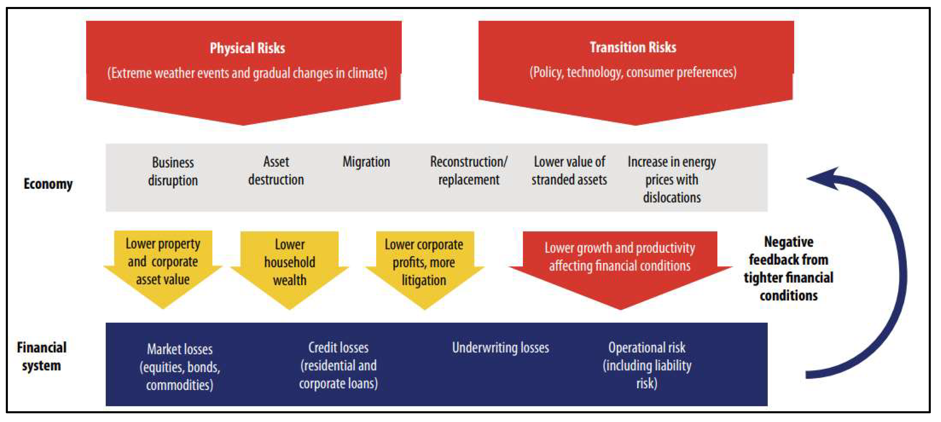The 2019 climate report by the IMF [8] finds climate change to impact negatively on the financial system via two main channels (see Figure 1). The first route is physical risks, which occur from harm to infrastructure and land properties. The second occurs through transition risk due to variations in climate policy, technology, and consumer sentiments in the energy transition process. Exposures to financial risk can manifest directly in corporations facing climatic shocks. Financial risk can equally happen indirectly via climate change shock on the financial system [9,10]. Exposures appear as a higher default risk for loan portfolios or declining asset values. Studies have found cases of natural disaster losses across the globe, causing insurance costs to increase. Corporations whose operational models neglect the economics of low-carbon emissions risk heavy losses and eventual collapse [10,11].

Financial risk can create financial sector instability which will have negative consequences on green technology investment funding. In periods of intense pollution, the financial sectors’ support of abatement processes promotes environmental sustainability [3]. A recent study by [12] established that reducing financial risk helps in controlling CO₂ emissions in the OECD member economies. This finding suggests global economies must take prudent financial risk management policy measures towards economic stabilization that ensure improvements in environmental quality and control of climate change. The lingering academic question relates to the global validity of these empirical findings since limited studies have been observed in the literature. To establish validity in this empirical claim, the case of Poland presents a fertile ground for investigation due to their historically checkered financial risk records, nature of pollution policies, and environmental quality records among peers in the European Union.

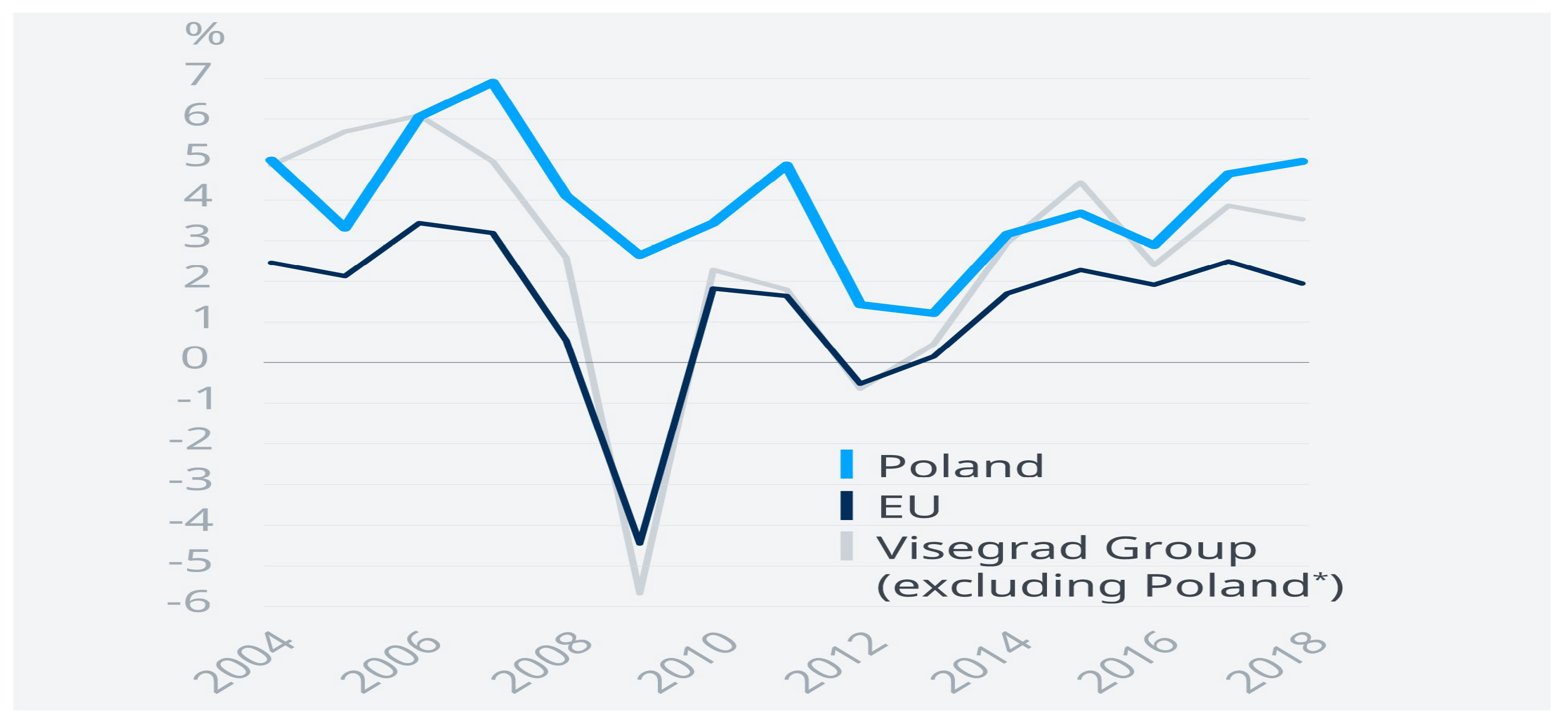
With its 2022 population at 37.8 million, and a per capita of USD 17,946, the Polish economy has had impressive economic growth over the last two decades. Annual GDP growth in Poland averaged 3.99 percent between 1996 and 2018, reaching as high as 7.10 percent in 2007, according to an OECD report. Quality of life in Poland has improved considerably, as reflected in their global well-being scores such as the recent ratings by the Better Life index of the OECD, 2022. The Polish economy has an enviable and improved business climate, facilitating its leading position in World Bank’s Doing Business ranking report among the EU and OECD peers in reforms, and it possesses a healthy utility-like banking sector. Figure 2 illustrates historical records of Polish real GDP growth (%) since joining the EU.

The country’s sovereign credit rating is low. Sovereign credit ratings are an assessment of the ability and willingness of sovereign states to honor debt obligations [13]. They are an important piece of information for international investors and affect the borrowing costs of debt-defaulting countries. A fast-changing corporate environment demands financial stability and liquidity, which pivots into the ability of corporations to control financial risk. The financial sector reforms by Poland insulated the country’s corporations from the ills of the 2007–2008 global financial crisis [14]. However, recent events in the Euro-area due to the Ukraine-Russia geopolitical war and the energy sector crisis have affected the financial stability of Poland, resulting in increasing inflation, rising interest rates and financial market repricing. In addition, the monetary policy actions by the Polish Central Bank have contributed to tighter financial conditions and increased financial market volatility. Further, recent asset price shifts reflect increasing monetary policy uncertainty to moderate inflation; and the mix of high inflation outturns and rising interest rates have continued to weigh on Poland’s recent economic growth rate.

In environmental performance, Poland is a net energy importer. Beginning in 2004, when it joined the EU, Poland constructed more water treatment plants, tried to reduce CO₂ emissions by over 30% compared to 1990 levels, and implemented several policies on endangered plant and animal species. Additionally, Poland underperforms the average in terms of health and environmental quality, although performs well in several well-being metrics when compared to other countries (such as education and social ties). The quantity of PM2.5 (small air pollution particles) in the atmosphere is 22.8 micrograms per cubic meter, more than the OECD average; approximately 18% of Polish people are unhappy with the quality of their water (Better Life Index, 2023). Poland’s coal industry continues to remain a significant component of the local economy after Germany, and this is the major source of air pollution.

Table 1. Environmental performance in Poland.

Environmental Factor	1995	2022
Carbon emissions per unit of GDP (PPP)	1.76%	0.54%
CO2 emissions (metric tons per capita)	8.94%	7.99%
Renewable energy consumption (% Total energy consumption)	4.61%	11.72%
Renewable electricity output (% total electricity output)	1.26%	13.8%
Biodiversity loss	30%	16%

Source: IEA Statistics and WorldBank.

illustrates the environmental performance of Poland between 1995 and 2022.

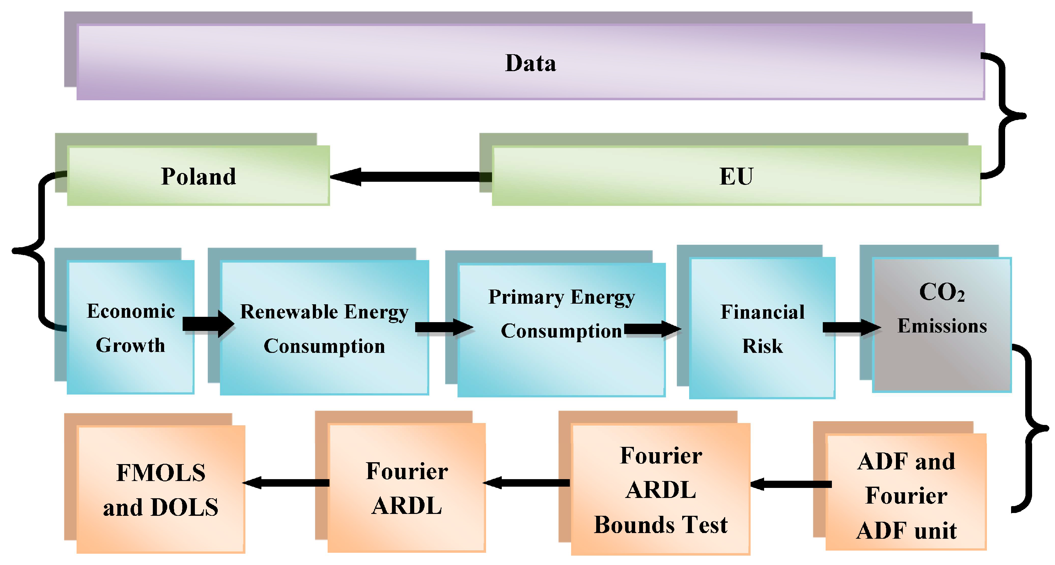
Based on this background, and since the industrial revolution, the global economy has faced the problem of global warming and environmental pollution. However, knowing that renewable technology is the savior pathway, increasing financial risk can affect research and development budgets, creating a block on our way to environmental sustainability. Limited by the literature on these relationships, this paper aims to accurately capture the effect of financial risk on environmental degradation in Poland from 1990Q1 to 2019Q4 while keeping economic growth, primary energy use, and renewable energy consumption under control. For reliable outcomes, the study employs Fourier-ARDL and Toda Yamamoto causality approaches. In contrast to previous research, this work employs a newly modified Autoregressive Distributive Lag (ARDL) cointegration test based on a Fourier function presented by [15]. In contrast to ARDL and DARDL methods, Fourier ARDL (FARDL) has several vital features [16,17,18]. First, variable integration levels are not required. Second, several seamless structural variations are easily detectable. Third, the estimator uses dummy variables to capture structural variations. The remaining sections of this paper are structured as follows: Section 2 conducts the literature review; Section 3 is a summary of the data, sources, and analytical methods employed; Section 4 illustrates and discusses empirical findings; and Section 5 closes the paper with policy suggestions.

2. Review of the Related Literature

This section is a comprehensive review of studies on the variables of interest and their relationship with environmental degradation. The review highlights relevant debates and gaps in studies linked with the purpose of the study. In the review process, four hypotheses are made:

Hypothesis 1 (H1).

Increasing financial risk reduces financing of economic growth, leading to a reduction in environmental degradation in Poland.

Historically, global economies have committed to taking steps towards carbon neutrality since the 2015 UN climate conference (COP21) in Paris, with huge budgetary allocations towards renewable energy technological development. However, economies with internal and external challenges and financial risks have different stories on realizing global climate goals. Expanding the financial system requires activity commodification based on financial judgments and traded assets. The effect of financial risk on environmental degradation has gained focus in scholarly research, albeit with contradictory outcomes. In their studies, they found that participative decision-making reduces corporate risk and helps corporations to advance superior environmental performance and corporate sustainability [19,20,21]. Ref. [22] studied 111 economies between 1985 and 2014 on the nonlinear effect of country risk on CO₂ emissions and found that financial risk positively affects environmental degradation across the panel. However, this result contradicted the study of [23] on CO₂ emissions in China, a result which validated the study by Ozturk and Acaravci (2013). However, in their recent study, [12] found financial risk causes CO₂ emissions to increase. Financial risks can create financial instability and impact environment-related investments. This will eventually affect environmental quality. In their study, [12] evidenced that this factor has historically been overlooked by researchers and claimed that reducing financial risk affects CO₂ in OECD. Based on this review, the paper considers that rising financial risk reduces the financing of economic growth, leading to a reduction in environmental degradation in Poland.

Hypothesis 2 (H2).

Renewable energy consumption exerts a negative effect on environmental degradation in Poland.

The global economy has accelerated investments in renewable energy because scientific evidence indicates its negative effect on both economic growth and environmental quality [24,25,26]. In relation to climate change, renewable energy use is validated for environmental sustainability through greenhouse gas emissions [27]. Other scholars have found the use of renewable energy to offer both environmental and economic advantages [28,29], including investment portfolio diversification, expanded energy mix, and employment opportunities. The literature on renewable energy and carbon emissions has mixed outcomes based on the methodology employed in country-specific contexts, and variable considerations [30]. While some studies find feedback causality between CO₂ emissions and renewable energy use [31,32], other studies find otherwise. For example, in the case of Thailand, the study by [33] found no evidential nexus between renewable energy use and CO₂ emissions. However, a study by [34] found that renewable energy exerted a negative effect on CO₂ emissions in 25 selected African economies between 1980 and 2012. In the case of the G-7 nations, [35] found that renewable energy use and energy price facilitated improvements in environmental quality. With this review information, the paper hypothesizes that renewable energy consumption exerts a negative effect on environmental degradation in Poland.

Hypothesis 3 (H3).

Increasing primary energy consumption facilitates rising environmental degradation in Poland.

It is generally found in the literature that economic growth is closely related to energy consumption [36,37,38]. This is based on the rising threats of global warming and climate change. Scholars hypothesize that increasing economic development requires more energy consumption or productivity of energy use [39,40]. A study by [41] in five ASEAN economies indicated that a statistically positive relationship existed between electricity consumption and carbon emissions non-linearly, consistent with the historical EKC hypothesis. It should be emphasized that economic theories are not explicit on the nexus between energy use, economic growth, and CO₂ emissions; recent studies have focused heavily on the Environmental Kuznets Curve (EKC) or the Carbon Kuznets Curve (CKC) hypothesis with some validation [42,42], invalidation [43,44], and inconclusive outcomes [45]. Another comparative study on wood, concrete, and steel utility poles indicated that wood poles had little environmental effect. In their life cycle assessment of primary energy use, [46] found that heating systems determine primary energy consumption and CO₂ emission; and that biomass-based heating systems and electricity cogeneration reduce primary energy use and CO₂ emissions. However, balancing information based on this review, the paper assumes that increasing primary energy consumption facilitates rising environmental degradation in Poland.

Hypothesis 4 (H4).

Increasing economic growth augments rising environmental degradation in Poland.

Historically, several studies have claimed an association between economic growth and CO₂ emissions [26,47,48]. Theoretically, EKC claims the existence of an inverted U-shaped relationship between environment and income. It states that environmental degradation increases up to some point—the turning point—as income increases. Yet after the turning point, this degradation decreases with an increase in income level [47]. The plotted graph between income and environmental degradation has an inverted U-shape. The study by [49] estimated the EKC for four environmental indicators along with nominal GDP in the late 1980s, and found that pollution reduction was possible with higher income levels since economic growth eventually improves environmental quality. The authors of [50] studied the relationship between economic growth and carbon emissions, and found that rising economic output causes destruction to the environment. The study by [51] in Mexico also found a positive association between CO₂ emissions and economic growth. In Turkey, [52] found that economic growth positively affected CO₂ emissions using wavelet coherence approaches. For the case of ASEAN economies, [53] assessed how economic growth related to CO₂ emissions with data between 1971 and 2017. The outcomes indicated that rising economic growth destroyed selected economies in terms of carbon emissions. Based on this, this study assumes that increasing economic growth augments rising environmental degradation in Poland.

Given this in-depth literature review, the effect of financial risk on environmental degradation has not been exhaustive. Similarly, the review has indicated that both primary energy consumption and economic growth are projected to exert a positive effect on environmental degradation in Poland, while financial risk and renewable energy are tipped to have a negative effect on environmental degradation in Poland. Given the limitations of recent empirical investigations determining factors affecting environmental degradation in Poland, this study employs novel Fourier-based ARDL and Fourier Toda Yamamoto causality estimators for its analysis. These methods have been validated to provide accurate and reliable policy-sensitive outcomes [54].

3. Methodology

3.1. Data and Sources

This research aims to detect the effect of financial risk on environmental degradation in Poland by keeping in check the role of economic growth, primary energy use, and renewable energy consumption between 1990Q1 and 2019Q4. All variables are in log form. Data were taken on (i) GDP per capita (GDP, in constant 2015 USD to serve as a proxy variable for economic growth); data was sourced from the World Bank database, 2020. According to [54], economic growth refers to an increase in an economy’s production and consumption of both economic products and services. GDP per capita is calculated by dividing the total gross value contributed by all producers who are residents of the economy by the mid-year population, plus any product taxes (fewer subsidies) that are not considered when valuing output; (ii) CO₂ emissions were sourced from UNFCC as a proxy for environmental degradation. Carbon dioxide is a gas generated by the burning of carbon, and by living organisms as they respire. Carbon dioxide is measured in parts-per-million (ppm); (iii) Data on financial risk were sourced from PRS Group. Experts define financial risk to refer to the probability of financial loss [6,7]. Financial risk is a term used to refer to a corporation’s inability to manage and fulfill its financial obligations due to economic instabilities and market losses which culminate in business collapse. This has been found to have profound environmental consequences [55]. Financial risk is measured in various ways, such as total assets to shareholder’s equity ratio; debt to equity ratio; debt to income ratio, etc. (iv) Data on renewable energy was gathered from the OECD; consumption of renewable energy (RE) is assumed to reduce carbon emissions. The utilization of renewable energy is calculated as the total energy used for growth activity divided by the total energy used from renewable sources. This energy comprises solar and wind energy, which is regenerated naturally. Information was obtained from the International Energy Agency’s database; (v) Data was sourced on primary energy consumption (PEC) from OECD. Primary energy [56] is measured in terawatt-hours (TWh). It is the direct consumption of sources of energy without transformation or a conversion process. Given that scaling problems exist, the present study avoids this by transforming variables into their natural logarithm forms except for renewable energy consumption (RE) [57].

Table 2. Time Series Variables.

Variable	Role in the Model	Source
Carbon dioxide emissions (CO2E)	Dependent variable	[58]
GDP per capita (GDP)	Controlled independent variable	[54]
Primary energy consumption (PEC)	Controlled independent variable	[56]
Renewable energy consumption (RE)	Controlled independent variable	[58]
Financial Risk (FRI)	Controlled independent variable	[12]

lists variables of interest for the empirical study, and Figure 3 is the methodological flowchart.

3.2. Theoretical Motivation

All economies in the world strive for economic growth, which comes along with significant environmental threats to human lives [59]. The United Nations and other global environmental organizations are looking for strategies to deal with the threat posed by environmental degradation from economic growth. Dealing with financial risk is one of the main pathways that scientists have proposed. Similarly, experts have discovered that environmental degradation is closely related to primary energy and renewable energy use [54,60]. Based on the literature review, both primary energy consumption and economic growth are projected to exert a positive effect on environmental degradation in Poland, while financial risk and renewable energy are tipped to have a negative effect on environmental degradation in Poland. Unlike previous theoretical frameworks, this study utilizes the Kindergarten Rule model by [61], which emphasizes the role of technology advancement in pollution abatement and the beneficial role of knowledge spill-over effects. Under this framework, there is an expectation for gradual adjustments in productivity abatements due to the role of knowledge capital accumulation which occurs instantaneously. This model can also decompose or distinguish between the composition of output, its scale, and per unit output emissions.

There are two contributions that this Kindergarten Rule model can make to the literature and policy. First, it shows how technical improvements in abatement can reduce compliance costs despite ongoing economic expansion. If abatement is effective, sustainable growth can be achieved without increasing compliance costs. Using this model, the paper illustrates the importance of making technological growth endogenous by focusing on reducing emissions. Second, much like the [62] model and the EKC concept put forth by [47], the Kindergarten Rule model illustrates an initial deteriorating environment that improves over time; a paradigm explaining why the relationship between income and pollution differs systematically between economies.

The algebra linking emissions of a pollutant to a measure of economic activity, its composition, and the cleanliness of production techniques are modeled as regime shifting ecosystems by-product of all production as

$$E={\displaystyle \sum }_{i=1}^n{a}_i{s}_{i}Y, \mathrm{where} {\displaystyle \sum }_{i=1}^n{a}_i=1$$

(1)

where E denotes the total pollutant emissions arising from production across the economy; n is industries; a_i denotes emissions per dollar of output produced in the industry _i, s_i denotes the value share of industry _i in national output; and Y denotes total national output. By differentiating both sides regarding time, the model becomes

$$E={\displaystyle \sum }_{i=1}^n{\pi }_i \left\{{\widehat{a}}_i {\widehat{s}}_i\right\}+Y, \mathrm{where} {\pi }_i=\frac{E_i}{E}$$

(2)

where $\widehat{a}$ over x indicates [dx=dt]/x. Changes in aggregate emissions can arise from three sources that are denoted to be scale, composition, and technology effects.

By modeling the environment as a sink for human wastes, the assumption is made that both emissions with natural regeneration determine environmental quality. This means by adjusting the environment to changes in levels of pollution, natural regeneration could determine environmental quality. Here, since emissions over time is E, the pollution stock evolution is given by

$$X=E-\eta X \mathrm{where} \eta >0$$

(3)

where X is assumed to be bounded for human life to exist, and there is a simple negative linear relationship between the steady-state generation of pollution E and the pollution stock X.

All work requires energy, and energy is always wasted in the work process as the unintentional by-products of production, known as pollution; as such, assumed as

$$i,t\ge 0, lim, in f \left[a, \left(t\right)\right]>0$$

(4)

implying that for each _i, a is strictly positive “>0 such that a_i(t)>”. It also implies that the composition effects are a transitory process to lower pollution emissions as

$$E \left(t\right)\le B\Rightarrow {\displaystyle \sum }_{t=1}^{n}a,\left[t\right] s,\left[t\right] \le \frac{B}{Y\left[t\right]} \mathrm{for} \mathrm{all} t\ge 0$$

(5)

However, if the world is to emit with growing Y(_t), the cleanest industry emission rate a_i(t) should be trending towards zero. Hence, falling pollution levels and rising incomes are only possible if there are continual reductions in emissions per unit output and if zero emission technologies are possible, as denoted by

$$\stackrel{*}{a}\left(t\right)≔\left(a,\left[t\right]\right)\le \frac{B}{Y\left[t\right]} \to 0 as t \to \infty$$

(6)

3.3. The Model and Econometric Approach

The model to determine the factors determining carbon emissions in Poland is written as:

CO_2t = f(GDP, RE, PEC, FRI)

(7)

where CO₂ is carbon dioxide emissions; GDP is GDP growth; RE is renewable energy consumption; PEC is primary energy consumption; FRI is financial risk; and e_t is the error term.

By taking the natural log of the variables except RE, the independent variables affecting the dependent variable of the model become specified as

LCO_2it = α₁ + β₁LGDP_it + β₂RE _it + β₃LPEC _it + β₄LFRI _it + e_ti

(8)

where the dependent variable responds to independent variables; LCO₂ is the natural log value of carbon dioxide emissions; LGDP is the natural log value of GDP growth; RE is renewable energy consumption; LPEC is the natural log value of primary energy consumption; and LFRI is the natural log value of financial risk; α is constant; i refers to economy, t is time; and e_t is the error term.

In recent econometric analysis, researchers have found that variances over time occur and as such are non-stationary, normally resulting in spurious regression. This study uses Augmented Dickey-Fuller (ADF) unit root tests with a breakpoint in assessing the variables integration order. The study estimates unit roots for ADF with breaks, expressed as:

$$X_t=\mu +\rho x_{t-1}+e_t$$

(9)

here, x_t refers to variables of interest; μ is the constant term; and e_t the error term. By unit differencing, the model becomes Δx_t = μ + e_t; where Δ = (1 − B); ρ refers to parameter slopes for lagged variables and becomes 1 whenever there occurs a unit root. The study illustrates the alternative unit root for ADF with breaks and the Fourier unit root, written, respectively, as

$$X_t=\mu +{\beta }_t\delta DU+\theta D {\left\{T_B\right\}}_t+e_t$$

(10)

$$X_t=\mu +{\beta }_t+{\gamma }_{1}cos \lceil \frac{2r{k}_t}{N}\rceil +{\gamma }_{2}sin \lceil \frac{2r{k}_t}{N}\rceil +e_t$$

(11)

where β refers to parameter slopes; k refers to frequency; γ refers to slope parameter in the Fourier function; the trend is t; N refers to observations; π = 3.1416; δ is the structural break dummy parameter slope. DU_t = 1, if t > T_B and DU_t = 0, if otherwise, T_B is breakpoints” [63]; θ is the slope parameter for the one-time break dummy, and D(T_B)_t = 1 if t = T_B and D(T_B)_t = 0 if otherwise.

In the post re-specifications of error correction form, and after applying the augmentation factor, the ADF with breaks equation is estimated as:

$$\Delta x_t=\mu +{\beta }_t+{\gamma }_{1}cos\lceil \frac{2r{k}_t}{N}\rceil +{\gamma }_{2}sin\lceil \frac{2r{k}_t}{N}\rceil +\left\{\rho -1\right\} x_{i-1}{{\displaystyle \sum }}_{i-1}^p{c}_i\Delta x_{i-1}+e_t$$

(12)

Here, c refers to slope parameter of the augmented parts; p is the lag length with minimum information criteria values in the augmentation process; k is Fourier regularity.

Fourier ARDL long-run cointegration estimation.

In modern econometrics, positive and negative shocks are to be determined to accurately detect hidden long-run cointegration. While the Fourier function helps, it also facilitates the detection of structural changes, despite it not being a requirement for cointegration assessment. The Fourier-based ARDL approach, according to [15,16,17,18,19,20,21,22,23,24,25,26,27,28,29,30,31,32,33,34,35,36,37,38,39,40,41,42,43,44,45,46,47,48,49,50,51,52,53,54,55,56,57,58,59,60,61,62,63], offers a more reliable long-term cointegration estimation outcome than the typical ARDL methodologies. The Fourier function helps to identify structural changes in the model.

$$d\left(t\right)={\displaystyle \sum }_{k=1}^n{a}_{\mathrm{k}}\sin \left(\frac{2\pi kt}{T}\right)+{\displaystyle \sum }_{k=1}^n{b}_{\mathrm{k}}\cos \left(\frac{2\pi kt}{T}\right)$$

(13)

where ‘n’ indicates the number of frequencies; π = 3.14, ‘k’ is the number of special frequencies selected; ‘t’ is the trend; and ‘T’ is the sample size. A single frequency value is used as

$$d\left(t\right)=\gamma 1sin\left(\frac{2\pi kt}{T}\right)+\gamma 2cos\left(\frac{2\pi kt}{T}\right)$$

(14)

The FARDL model for this study is shown as

$$\begin{array}{cc}\hfill \Delta LCO2\mathrm{t}=\beta 0+& \gamma 1sin\left(\frac{2\pi kt}{T}\right)+\gamma 2cos\left(\frac{2\pi kt}{T}\right)+\beta 1LCO2\mathrm{t}-1+\beta 2LGDP\mathrm{t}\hfill \\ & -1+\beta 3RE\mathrm{t}-1+\beta 4LPEC\mathrm{t}-1+\beta 5FRI\mathrm{t}-1\hfill \\ & +{\displaystyle {\displaystyle \sum }_{i-1}^{\rho -1}}\phi \mathrm{i}\prime \Delta LCO2\mathrm{t}-\mathrm{i} +{\displaystyle {\displaystyle \sum }_{i-1}^{\rho -1}}\delta \mathrm{i}\prime \Delta LGDP\mathrm{t}-\mathrm{i} +{\displaystyle {\displaystyle \sum }_{i-1}^{\rho -1}}\varnothing \mathrm{i}\prime \Delta RE\mathrm{t}-\mathrm{i} \hfill \\ & +{\displaystyle {\displaystyle \sum }_{i-1}^{\rho -1}}\vartheta \mathrm{i}\prime \Delta LPEC\mathrm{t}-\mathrm{i} +{\displaystyle {\displaystyle \sum }_{i-1}^{\rho -1}}\vartheta \mathrm{i}\prime \Delta FRI\mathrm{t}-\mathrm{i}+e\mathrm{t}\hfill \end{array}$$

(15)

Ref. [15] used a bootstrap simulator and the frequency value at the minimum squared sum of residuals.

Last, this study employs the Fourier Toda Yamamoto Causality Test to check the causality linkage among the time series variables. Compared to the traditional Granger-based causality test, this approach is more accurate and gives reliable results.

4. Empirical Outcomes, Analysis and Discussions

This study attempts to establish the consequences of financial risk on environmental deterioration in Poland from 1990Q1 to 2019Q4 by keeping economic progress, primary energy consumption, and renewable energy usage in a controlled position. The variables examined in this inquiry are listed and explained in

Table 3. Descriptive Statistics.

	LCO2	LFRI	LGDP	RE	LPEC
	Production-Based CO2 Emissions	Financial Risk Index	GDP (Constant 2015 USD)	Renewable Energy Consumption	Primary Energy Consumption
Mean	5.496330	3.603264	11.50942	7.895163	3.047283
Median	5.491481	3.637586	11.50677	7.303030	3.050621
Maximum	5.552000	3.839452	11.76296	12.73920	3.084789
Minimum	5.454142	3.106080	11.25612	1.652488	2.998265
Std.Dev.	0.028814	0.127434	0.150400	2.796168	0.022802
Skewness	0.552868	−1.007030	−0.121308	−0.267870	−0.415231
Kurtosis	2.035459	4.953997	1.808050	2.546615	2.467450
Jarque-Bera	10.76496	39.37273	7.398036	2.462881	4.866379
Probability	0.004596	0.000000	0.024748	0.291872	0.087757

Note: LCO₂ is log of carbon emissions; LFRI is log financial risk; LGDP is log of GDP growth as a proxy for economic growth; RE is log of renewable energy consumption; and LPEC is log of primary energy consumption.

.

The outcomes of the descriptive assessment (Table 3) show no outliers in the dataset. The outcomes also indicate variables are normally distributed, paving the way for further estimation activity. The next step in the pre-estimation process is assessing the unit root properties of the variables considered for the study.

The initial assessment of this paper checks the integration properties of interest variables by employing ADF unit root with breakpoint methods. It must be stressed that structural breaks have historically been ignored in econometric analysis, and this has caused biased unit root outcomes. Before assessing the integration order of the variables, this study uses the [64] BDS test to detect nonlinear patterns (i.e., dependence or independence). It is applied to assess varied embedding dimensions, ranging from 2 to 6, and it possesses several advantages over other alternatives. First, it is used to guide against model misspecification. Second, it helps to guide against making judgmental errors. The econometric application is defined as:

$$BD{S}_{mT}^{ }(\varepsilon )=T^{1/2}[C_{m,T}^{ }(\varepsilon )- C_{1,T}^{ }{(\varepsilon )}^m]/{\varepsilon }_{mT}(\varepsilon )$$

(16)

Here, T is the sample size; ɛ is a randomly selected proximity parameter; and ${\delta }_{mT}$(ɛ) is the standard deviation of the statistic’s numerator, which changes with dimension “m”.

The BDS estimates (

Table 4. BDS Test.

LCO2
Dimension	BDS Statistic	Std. Error	z-Statistic	Prob.
2	0.191686	0.005844	32.79952	0.0000 *
3	0.323752	0.009320	34.73713	0.0000 *
4	0.413098	0.011134	37.10344	0.0000 *
5	0.473033	0.011640	40.63862	0.0000 *
6	0.513248	0.011259	45.58593	0.0000 *
LFRI
Dimension	BDS Statistic	Std. Error	z-Statistic	Prob.
2	0.160470	0.008094	19.82701	0.0000 *
3	0.263424	0.012954	20.33598	0.0000 *
4	0.324945	0.015536	20.91583	0.0000 *
5	0.358126	0.016310	21.95776	0.0000 *
6	0.368470	0.015843	23.25733	0.0000 *
LGDP
Dimension	BDS Statistic	Std. Error	z-Statistic	Prob.
2	0.202515	0.003791	53.42304	0.0000 *
3	0.343083	0.006037	56.83338	0.0000 *
4	0.441978	0.007198	61.39902	0.0000 *
5	0.512476	0.007511	68.22775	0.0000 *
6	0.563894	0.007251	77.77128	0.0000 *
RE
Dimension	BDS Statistic	Std. Error	z-Statistic	Prob.
2	0.188066	0.005566	33.79116	0.0000 *
3	0.314690	0.008840	35.59738	0.0000 *
4	0.400087	0.010518	38.03869	0.0000 *
5	0.460339	0.010952	42.03373	0.0000 *
6	0.503868	0.010550	47.75962	0.0000 *
LPEC
Dimension	BDS Statistic	Std. Error	z-Statistic	Prob.
2	0.176395	0.005670	31.10910	0.0000 *
3	0.292925	0.009044	32.38727	0.0000 *
4	0.365634	0.010806	33.83538	0.0000 *
5	0.409492	0.011299	36.23997	0.0000 *
6	0.434783	0.010931	39.77460	0.0000 *

Stars * denote the level of statistical significance at 1%.

) show there are hidden nonlinear patterns in the time series data, and all variable values have “dimensional critical values” that are higher than the BDS estimates. This implies the existence of a nonlinear correlation between all variables.

The research then uses the Fourier ADF and ADF with breaks unit root tests to evaluate the unit root qualities of variables. However, before applying the Fourier ADF (FADF) unit root estimator, it is essential to investigate the Fourier function’s impact and determine its statistical significance. Results from the ADF with Break Point and FADF tests are illustrated in

Table 5. Fourier ADF and ADF Unit Root Tests.

Variable	F-STAT	FADF	ADF with Break Point
LCO2	2.022332		−4.321 * (1997Q1)
RE	2.739148		−3.509 (2007Q4)
LGDP	2.035628		−2.494 (1991Q4)
LFRI	4.368201 **	−4.423201 **
LPEC	2.448424		−3.364 (2009Q1)
DLCO2			−4.688 ** (1992Q1)
DRE			−10.587 *** (1993Q1)
DLGDP			−6.186 *** (2012Q1)
DLFRI
DLPEC			−5.626 *** (1992Q1)

Stars ***, **, * denote the levels of statistical significance at 1%, 5%, and 10%, respectively.

.

The results (Table 4) indicate that both LCO₂ and LFRI time-series variables were integrated at level (I(0)); while RE, LPEC and LGDP were integrated at the order one, showing several breakpoints in 1991Q4, 1992Q1, 1993Q1, 1997Q1, 2007Q1, 2009Q1 and 2012Q1, respectively, at 1%, 5% and 10% statistical significance levels. The mixed order of integration of the variables is recognized per the results. This makes it possible to employ Fourier ARDL-based models for the next action. However, based on the estimates, decisions are made on the ADF unit root with breaks. The article next investigates the cointegration between the chosen variables to ascertain how LFRI and the controlled variables individually and collectively affect LCO₂ in Sweden. These results validate recent research by [65].

This study subsequently employs the Fourier-based ADL cointegration test to assess the cointegration attributes of the time-series variables, since the results show that the model is stable and does not exhibit serial autocorrelation or heteroscedasticity. Regardless of the variable integration order (I(0) or I(1)), the F-ADL test remains valid [66]. The estimator can also use linear processes to analyze the unrestricted error correction model. Since endogenous problems cannot alter the size and power features of the Bounds test, ARDL limits can be determined in the short run and the long run utilizing an asymptotic threshold of Monte Carlo simulations.

A long-run cointegration relationship may be discovered utilizing the Fourier ADL cointegration techniques, as seen in

Table 6. Fourier ADL Cointegration Test.

Model	Test Statistics	Frequency	Min AIC
LCO2 = f(LGDP, LFRI, LPEC, RE)	−8.5659 ***	1	−2.162648

Note: *** denotes statistically significant at the 1% level.

, where the t-statistical value is significant at 10% and indicates a cointegration relationship among the variables. With this outcome, there is a sense of long-run linkage between LCO₂, LGDP, LPEC, RE, and LFRI. The Fourier ARDL estimator is then used in the current study to quantify the individual or collective effect of LCO₂, LGDP, LPEC, RE, and LFRI on LCO₂ in Poland. Consideration is given to LGDP, LPEC, and RE, which were controlled to accomplish this paper.

The Fourier ARDL Long Run Form (

Table 7. Fourier ARDL Long Run Form.

Variable	Coefficient	Std. Error	t−Statistic	Prob.
LPEC	0.726834	0.224605	3.236057	0.0017
LGDP	0.669602	0.404350	1.655996	0.1010
RE	−0.008785	0.007394	−1.188029	0.2378
LFRI	−0.135554	0.060509	−2.240213	0.0274
C	−0.377313	0.096858	−3.895544	0.0002
TREND	−0.000143	3.70 × 10−5	−3.864089	0.0002
SIN	0.000610	0.000306	1.995073	0.0489
COS	0.000254	0.000315	0.807008	0.4217
CointEq(−1)	−0.055952	0.014380	−3.891103	0.0002

) estimates indicate that the coefficients of LPEC and LGDP are positive and significant. Moreover, the estimated coefficients of RE and FRI are negative but significant.

These indicate that a 1% increase in both LPEC and LGDP encourages a positive effect on LCO₂ by approximately 72.68% and 66.96, respectively. These Fourier ARDL Long Run Form estimation outcomes validate the hypothesis on both variables established for this study (i.e., Hypotheses 3 and 4). The results support [60]. It must be emphasized that, theoretically, rising economic growth affects environmental degradation due to increasing demand for natural resources and energy consumption. Depending on the models for such assessment, there is always an initial phase of environmental destruction before environmental regulatory and technology effects set in, which is popularly known as the EKC curve. This has been demonstrated extensively by all growth models, including the Source-and-Sink framework [67]; Solow model; and Smulders and Stokey’s AK theoretical model.

GDP growth over the last decade in Poland has been phenomenal and has undoubtedly caused carbon emissions to rise. The Polish economy has witnessed some level of deterioration due to the war in Ukraine in 2022, despite a strong post-COVID-19 rebound of 5.9% rise in real GDP growth in 2021. Economic activity has seen cooling supply-chain disruptions worsened by rising input costs—a direct outcome of globally surging energy prices. Over the last two decades, despite the historical records of rising growth and increasing carbon emissions, the current pent-up consumer-level spending and strong investment action with support from Next Generation EU funds, experts forecast a further projected rise in carbon emissions in Poland.

For primary energy consumption (i.e., fossil fuels, nuclear energy, and renewable sources of energy), Poland recorded 1.95% in 1996 to 8.79% in 2021. In nominal terms, the country saw a rise in primary energy consumption, from 19 Twh in 1990 to 44 Twh in 2021. The country recorded 79% in 2021 consumption of coal and lignite to maintain its power plants, with only an industrial share of a marginal 5%. The domination of coal in the power sector of Poland makes it the largest source of greenhouse gas emissions. It is not a wonder that one percentage change in primary energy use in Poland caused a whopping 7.26% upward adjustment in carbon emissions for the period, an outcome that validates the hypothesis established for this paper. This outcome supports [68], who found a similar trend and recommended that in Poland, carbon emissions from road transport could be significantly lowered by prioritizing renewable energy sourcing.

Additionally, the Fourier ARDL Long Run Form estimates indicate that a 1% rise in both LFRI and RE exerts a negative effect on environment degradation by 0.0008% and 13.55%, respectively. These estimates confirm hypotheses 1 and 2 established for this paper in the literature review process. The results support [5]. In their study, [12] revealed that rising financial risk helps reduce carbon dioxide emissions directly and could similarly have an indirect negative effect on carbon emissions through the facilitation of technological advancement. However, they also found the effect of financial risk on carbon emissions to be heterogeneous across the globe. In Poland, the Polish business environment is not too much at risk, despite perceived weakening recently. The proprietary environmental sustainability index of Allianz International Corporation places Poland at 54 out of 210 global economies. This reflects the strengths of Poland over energy consumption and CO₂ emissions (per GDP), water crisis, and general vulnerability to climate change.

For the case of renewable energy use, the outcome of the Fourier ARDL long form indicated reducing carbon emissions by −0.008785 percent, given a unit change in primary energy consumption in Poland. This outcome supports earlier findings by [69] and validates the hypothesis established in this study on renewable energy use in Poland. In his study, ref. [69] assessed costs and the potential of reducing greenhouse gas emissions in Poland by replacing fossil fuels using renewable energy technologies. The outcome indicated a fall in carbon dioxide emissions with reducing the cost of investment. The findings also validated the historical work of [69], who evaluated renewable energy sourcing and its effect on CO₂ emission in Poland. The outcomes of their investigations indicated renewable energy’s potential to reduce CO₂ emissions in Poland by about 40 million tonnes annually.

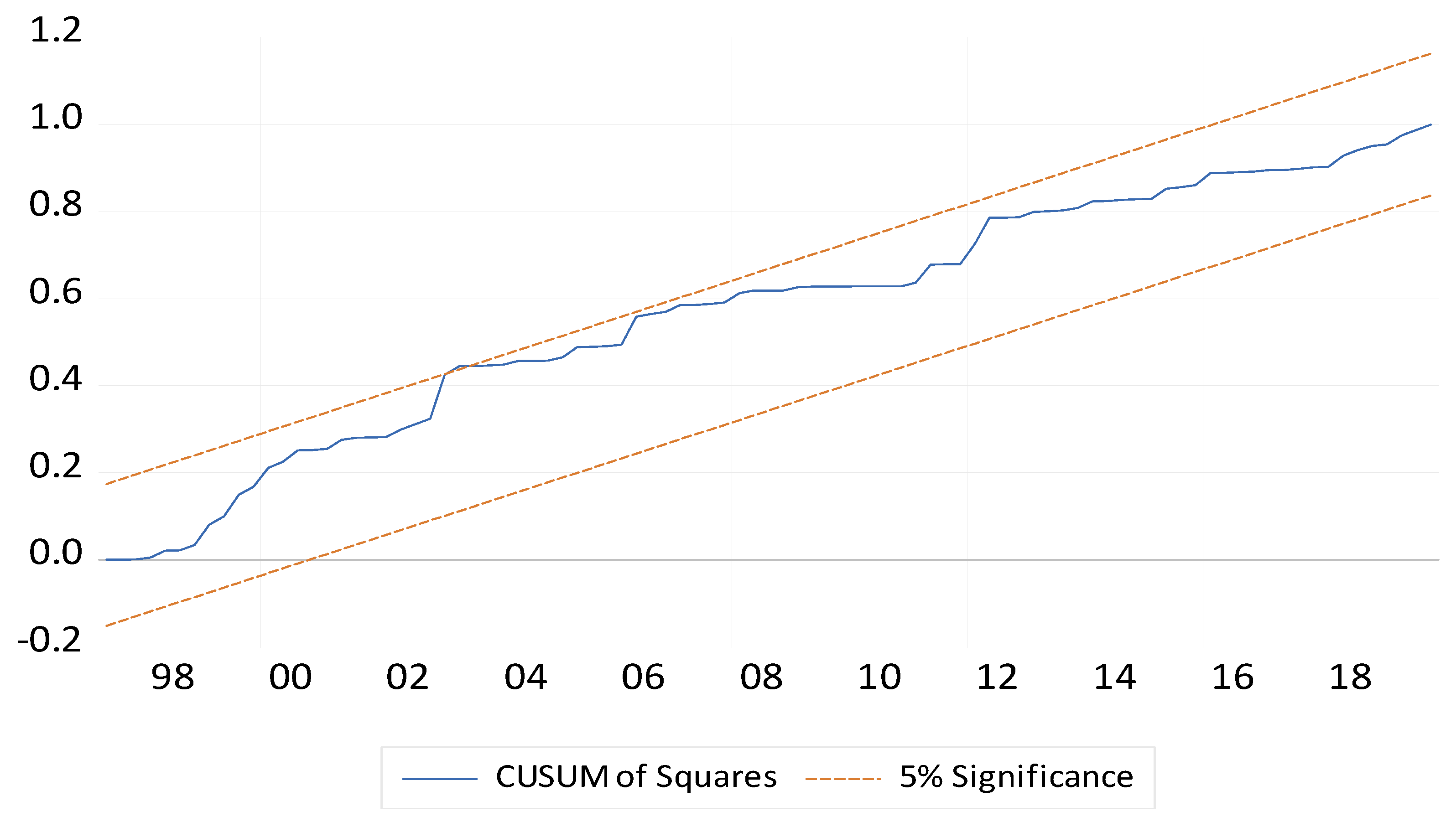
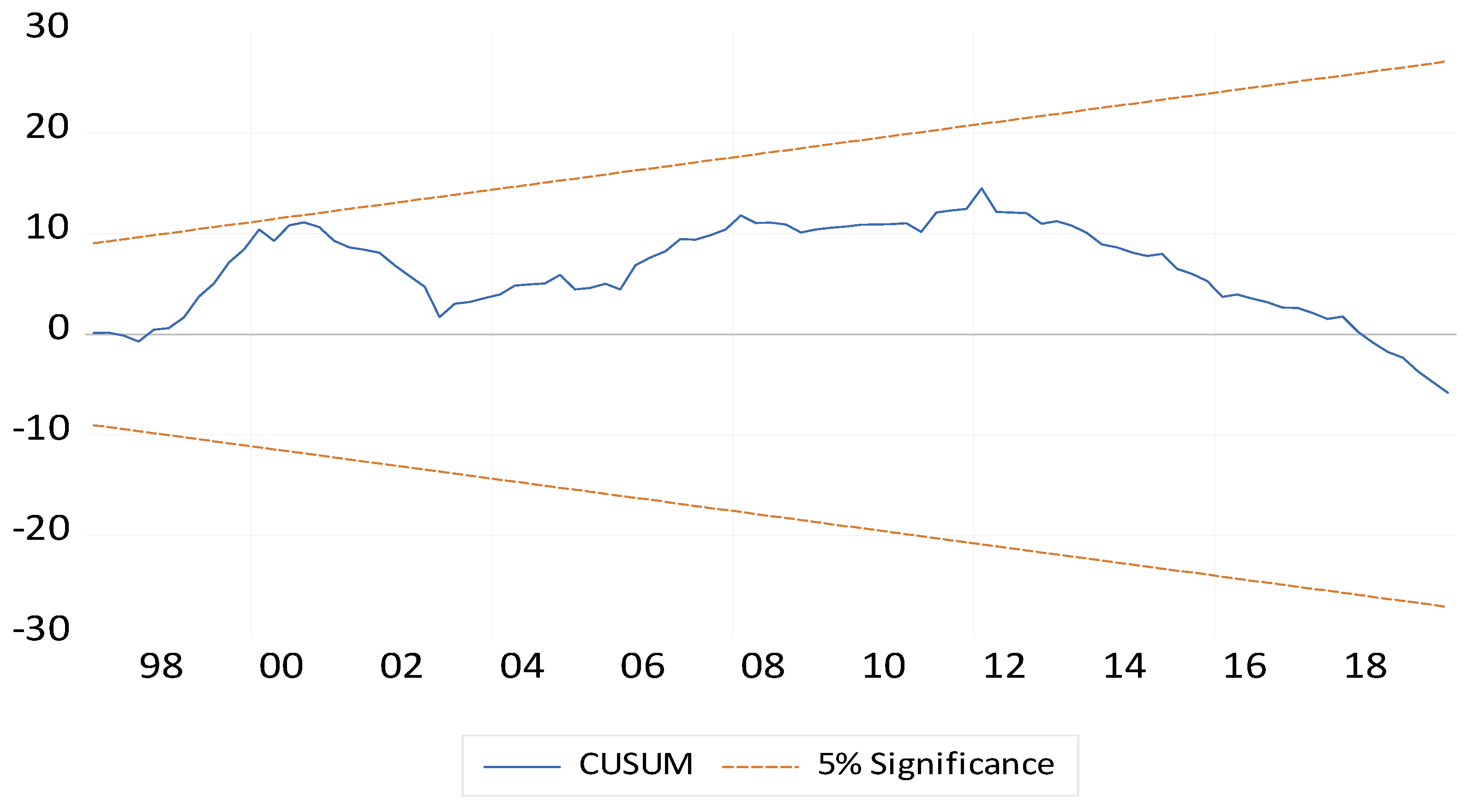
For reliable outcomes, this paper uses CUSUM and CUSUM of squares, Breusch-Godfrey serial correlation LM Test, and residual diagnostic test approaches, respectively, to capture the stability of the model and so the model is free from heteroskedasticity and serial correlation issues. In empirical evaluation, model stability and residual diagnostic tests are essential. To reduce LCO₂E, the coefficients in the error-correction model must be stable to serve as a guide for policy decisions on financial development, economic output, primary energy use, and the use of renewable energy sources for the case of Poland.

Figure 4 and Figure 5 illustrate the outcomes of cumulative stability test, while

Table 8. Heteroskedasticity Test: Breusch-Pagan-Godfrey.

Null hypothesis: Homoskedasticity
F-statistic	0.986549	Prob.	0.4834

and

Table 9. Breusch-Godfrey Serial Correlation LM Test.

F-statistic

2.749340

Prob.

0.0691

demonstrate outcomes of both the Breusch-Godfrey serial correlation LM Test, and the residual diagnostic test, respectively. The CUSUM and CUSUM of squares results in Numbers 4 and 5 indicate that the statistical figures are within acceptable limits. This indicates that the error-correction model’s coefficients are stable and can inform policy choices regarding renewable energy consumption, primary energy use, economic output, and financial risk to lower carbon dioxide emissions in Poland.

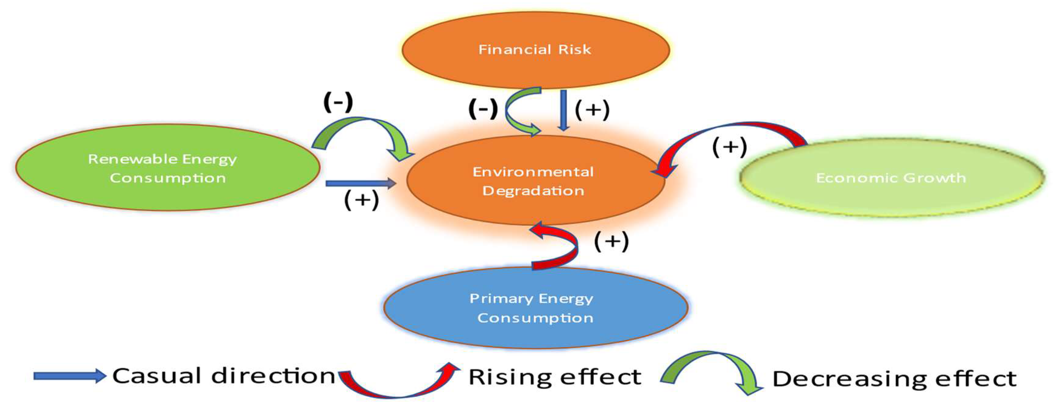
For better policy recommendations, it is vital—and a sufficient condition—to estimate the mutual causal linkages among the variables of interest. The Fourier TY Causality Test (

Table 10. Fourier TY Causality Test.

		T-Stat	p-Value
H1	REC does not cause LCO2E	10.05830 **	0.0425
H2	LFRI does not cause LCO2E	9.311705 *	0.0537
H3	LGDP does not cause LCO2E	2.569161	0.632296
H4	LPEC does not cause LCO2E	2.332299	0.506361

Note: * and ** denote statistically significant at the 10% and 5% levels, respectively.

) was used to assess the model. The outcome of the Fourier TY Causality Test indicates both LFRI and RE have a one direction causal effect on LCO₂, and there is no rebound action (Figure 6).

5. Conclusions and Policy Implications

This paper seeks to detect the effects of financial risk on environmental sustainability in Poland between 1990Q1 an 2019Q4. Economic output, primary energy utilization, and renewable energy usage are controlled. The outcomes indicate all variables are cointegrated, according to the Fourier ADL cointegration estimator. In addition, the Fourier ARDL long-form estimates demonstrate (i) both renewable energy and financial risk contribute to reducing environmental degradation in Poland; (ii) Poland’s environmental degradation is significantly worsened by both primary energy use and economic expansion, based on the Fourier ARDL long-form estimates; and (iii) analysis of the causality direction using the Fourier Toda Yamamoto Causality Test revealed that financial risk and renewable energy consumption over the period had a one-direction causal influence on LCO₂ without rebound effect in Poland.

To provide policy insights, this paper encourages the central bank to take actions supporting environmental policies that incorporate climate-related risks into supervision and financial stability monitoring. The Polish Central Bank may impose a requirement for financial institutions to include climate risk scenarios in their stress testing, given that changes in asset prices and catastrophic weather-related losses are preventable financial hazards. Finally, to increase investments in renewable energy technology, the European Union may offer the Polish government technical help regarding the macro-financial transmission of climate risks. This study has several limitations; like other investigative investigations. This paper concentrates on Poland, but could be extended to cover more economies and regions to enable comparisons to be made.

References

1. Nasir, M.A.; Huynh, T.L.D.; Tram, H.T.X. Role of financial development, economic growth & foreign direct investment in driving climate change: A case of emerging ASEAN. J. Environ. Manag. 2019, 242, 131–141. [Google Scholar]
2. Almond, J.; Sugumaar, P.; Wenzel, M.N.; Hill, G.; Wallis, C. Determination of the carbonyl index of polyethylene and polypropylene using specified area under band methodology with ATR-FTIR spectroscopy. e-Polymers 2020, 20, 369–381. [Google Scholar] [CrossRef]
3. Xue, C.; Shahbaz, M.; Ahmed, Z.; Ahmad, M.; Sinha, A. Clean energy consumption, economic growth, and environmental sustainability: What is the role of economic policy uncertainty? Renew. Energy 2022, 184, 899–907. [Google Scholar] [CrossRef]
4. Wang, Q.; Guo, J.; Li, R. Official development assistance and carbon emissions of recipient countries: A dynamic panel threshold analysis for low-and lower-middle-income countries. Sustain. Prod. Consum. 2022, 29, 158–170. [Google Scholar] [CrossRef]
5. Wang, Z.; Chandavuth, Y.; Zhang, B.; Ahmed, Z.; Ahmad, M. Environmental degradation, renewable energy, and economic growth nexus: Assessing the role of financial and political risks? J. Environ. Manag. 2023, 325, 116678. [Google Scholar] [CrossRef]
6. Wang, C.; Elfaki, K.E.; Zhao, X.; Shang, Y.; Khan, Z. International trade and consumption-based carbon emissions: Does energy efficiency and financial risk ensure sustainable environment? Sustain. Dev. 2022, 30, 1451–1461. [Google Scholar] [CrossRef]
7. Pan, K.; Cheng, C.; Kirikkaleli, D.; Genç, S.Y. Does financial risk and fiscal decentralization curb resources curse hypothesis in China? Analyzing the role of globalization. Resour. Policy 2021, 72, 102020. [Google Scholar] [CrossRef]
8. Grippa, P.; Mann, S. Climate-related stress testing: Transition risks in norway. In IMF Working Papers; International Monetary Fund: Washington, DC, USA, 2020. [Google Scholar]
9. Batten, S. Climate change and the macro-economy: A critical review. In Working Paper No. 706; Bank of England: London, UK, 2018. [Google Scholar]
10. Oguntuase, O.J. Climate change, credit risk and financial stability. In Banking and Finance; IntechOpen: London, UK, 2020; pp. 75–90. [Google Scholar]
11. Schumacher, I.; Strobl, E. Economic development and losses due to natural disasters: The role of hazard exposure. Ecol. Econ. 2011, 72, 97–105. [Google Scholar] [CrossRef]
12. Zhao, J.; Shahbaz, M.; Dong, X.; Dong, K. How does financial risk affect global CO2 emissions? The role of technological innovation. Technol. Forecast. Soc. Change 2021, 168, 120751. [Google Scholar] [CrossRef]
13. Kirikkaleli, D.; Gokmenoglu, K.K. Sovereign credit risk and economic risk in Turkey: Empirical evidence from a wavelet coherence approach. Borsa Istanb. Rev. 2020, 20, 144–152. [Google Scholar] [CrossRef]
14. Borscheid, P.; Haueter, N.V. (Eds.) World Insurance: The Evolution of a Global Risk Network; Oxford University Press: Oxford, UK, 2012. [Google Scholar]
15. Yilanci, V.; Pata, U.K. Investigating the EKC hypothesis for China: The role of economic complexity on ecological footprint. Environ. Sci. Pollut. Res. 2020, 27, 32683–32694. [Google Scholar] [CrossRef] [PubMed]
16. Danish, M.S.S.; Estrella, L.L.; Alemaida, I.M.A.; Lisin, A.; Moiseev, N.; Ahmadi, M.; Senjyu, T. Photocatalytic applications of metal oxides for sustainable environmental remediation. Metals 2021, 11, 80. [Google Scholar] [CrossRef]
17. Sofuoğlu, E.; Kirikkaleli, D. The effect of mineral saving and energy on the ecological footprint in an emerging market: Evidence from novel Fourier based approaches. Lett. Spat. Resour. Sci. 2023, 16, 3. [Google Scholar] [CrossRef] [PubMed]
18. Kirikkaleli, D.; Sofuoğlu, E. Does financial stability matter for environmental degradation? Geol. J. 2023. online version of record before inclusion in an issue. [Google Scholar] [CrossRef]
19. Kliestik, T.; Valaskova, K.; Lazaroiu, G.; Kovacova, M.; Vrbka, J. Remaining financially healthy and competitive: The role of financial predictors. J. Compet. 2020, 12, 74–92. [Google Scholar] [CrossRef]
20. Lăzăroiu, G.; Ionescu, L.; Andronie, M.; Dijmărescu, I. Sustainability management and performance in the urban corporate economy: A systematic literature review. Sustainability 2020, 12, 7705. [Google Scholar] [CrossRef]
21. Pocol, C.B.; Stanca, L.; Dabija, D.C.; Pop, I.D.; Mișcoiu, S. Knowledge co-creation and sustainable education in the labor market-driven university–business environment. Front. Environ. Sci. 2022, 10, 781075. [Google Scholar] [CrossRef]
22. Zhang, W.; Chiu, Y.B. Do country risks influence carbon dioxide emissions? A nonlinear perspective. Energy 2020, 206, 118048. [Google Scholar] [CrossRef]
23. Liang, S.; Zhang, T. What is driving CO2 emissions in a typical manufacturing center of South China? The case of Jiangsu Province. Energy Policy 2011, 39, 7078–7083. [Google Scholar] [CrossRef]
24. Al-Mulali, U.; Tang, C.F.; Ozturk, I. Does financial development reduce environmental degradation? Evidence from a panel study of 129 countries. Environ. Sci. Pollut. Res. 2015, 22, 14891–14900. [Google Scholar] [CrossRef]
25. Kahia, M.; Aïssa, M.S.B.; Lanouar, C. Renewable and non-renewable energy use-economic growth nexus: The case of MENA Net Oil Importing Countries. Renew. Sustain. Energy Rev. 2017, 71, 127–140. [Google Scholar] [CrossRef]
26. Raihan, A.; Muhtasim, D.A.; Pavel, M.I.; Faruk, O.; Rahman, M. Dynamic impacts of economic growth, renewable energy use, urbanization, and tourism on carbon dioxide emissions in Argentina. Environ. Process. 2022, 9, 38. [Google Scholar] [CrossRef]
27. Bhattacharya, M.; Churchill, S.A.; Paramati, S.R. The dynamic impact of renewable energy and institutions on economic output and CO2 emissions across regions. Renewable Energy 2017, 111, 157–167. [Google Scholar] [CrossRef]
28. Dai, H.; Xie, X.; Xie, Y.; Liu, J.; Masui, T. Green growth: The economic impacts of large-scale renewable energy development in China. Appl. Energy 2016, 162, 435–449. [Google Scholar] [CrossRef]
29. Spiegel-Feld, D.; Rudyk, B.; Philippidis, G. Allocating the economic benefits of renewable energy between stakeholders on Small Island Developing States (SIDS): Arguments for a balanced approach. Energy Policy 2016, 98, 744–748. [Google Scholar] [CrossRef]
30. Sinha, A.; Shahbaz, M.; Sengupta, T. Renewable energy policies and contradictions in causality: A case of Next 11 countries. J. Clean. Prod. 2018, 197, 73–84. [Google Scholar] [CrossRef] [Green Version]
31. Apergis, N.; Payne, J.E.; Menyah, K.; Wolde-Rufael, Y. On the causal dynamics between emissions, nuclear energy, renewable energy, and economic growth. Ecol. Econ. 2010, 69, 2255–2260. [Google Scholar] [CrossRef]
32. Sebri, M.; Ben-Salha, O. On the causal dynamics between economic growth, renewable energy consumption, CO2 emissions and trade openness: Fresh evidence from BRICS countries. Renew. Sustain. Energy Rev. 2014, 39, 14–23. [Google Scholar] [CrossRef] [Green Version]
33. Boontome, P.; Therdyothin, A.; Chontanawat, J. Investigating the causal relationship between non-renewable and renewable energy consumption, CO2 emissions and economic growth in Thailand. Energy Procedia 2017, 138, 925–930. [Google Scholar] [CrossRef]
34. Zoundi, Z. CO2 emissions, renewable energy and the Environmental Kuznets Curve, a panel cointegration approach. Renew. Sustain. Energy Rev. 2017, 72, 1067–1075. [Google Scholar] [CrossRef]
35. Ike, G.N.; Usman, O.; Alola, A.A.; Sarkodie, S.A. Environmental quality effects of income, energy prices and trade: The role of renewable energy consumption in G-7 countries. Sci. Total Environ. 2020, 721, 137813. [Google Scholar] [CrossRef] [PubMed]
36. Zhang, X.P.; Cheng, X.M. Energy consumption, carbon emissions, and economic growth in China. Ecol. Econ. 2009, 68, 2706–2712. [Google Scholar] [CrossRef]
37. Ozturk, I.; Acaravci, A. CO2 emissions, energy consumption and economic growth in Turkey. Renew. Sustain. Energy Rev. 2010, 14, 3220–3225. [Google Scholar] [CrossRef]
38. Zhang, M.; Song, Y.; Su, B.; Sun, X. Decomposing the decoupling indicator between the economic growth and energy consumption in China. Energy Effic. 2015, 8, 1231–1239. [Google Scholar] [CrossRef]
39. Narayan, P.K.; Narayan, S.; Popp, S. Does electricity consumption panel Granger cause GDP? A new global evidence. Appl. Energy 2010, 87, 3294–3298. [Google Scholar] [CrossRef]
40. Maji, I.K.; Sulaiman, C.; Abdul-Rahim, A.S. Renewable energy consumption and economic growth nexus: A fresh evidence from West Africa. Energy Rep. 2019, 5, 384–392. [Google Scholar] [CrossRef]
41. Lean, H.H.; Smyth, R. CO2 emissions, electricity consumption and output in ASEAN. Appl. Energy 2010, 87, 1858–1864. [Google Scholar] [CrossRef]
42. Xia, C.; Wang, Z. The effect of fossil fuel and hydropower on carbon dioxide emissions: EKC validation with structural breaks. J. Environ. Eng. Landsc. Manag. 2020, 28, 36. [Google Scholar] [CrossRef] [Green Version]
43. Murshed, M.; Ali, S.R.; Banerjee, S. Consumption of liquefied petroleum gas and the EKC hypothesis in South Asia: Evidence from cross-sectionally dependent heterogeneous panel data with structural breaks. Energy Ecol. Environ. 2021, 6, 353–377. [Google Scholar] [CrossRef]
44. Alola, A.A.; Donve, U.T. Environmental implication of coal and oil energy utilization in Turkey: Is the EKC hypothesis related to energy? Manag. Environ. Qual. Int. J. 2021, 32, 543–559. [Google Scholar] [CrossRef]
45. Rahman, A.; Murad, S.W.; Ahmad, F.; Wang, X. Evaluating the EKC hypothesis for the BCIM-EC member countries under the belt and road initiative. Sustainability 2020, 12, 1478. [Google Scholar] [CrossRef] [Green Version]
46. Gustavsson, L.; Joelsson, A.; Sathre, R. Life cycle primary energy use and carbon emission of an eight-storey wood-framed apartment building. Energy Build. 2010, 42, 230–242. [Google Scholar] [CrossRef]
47. Grossman, G.M.; Krueger, A.B. Economic growth and the environment. Q. J. Econ. 1995, 110, 353–377. [Google Scholar] [CrossRef] [Green Version]
48. Apergis, N.; Payne, J.E. CO2 emissions, energy usage, and output in Central America. Energy Policy 2009, 37, 3282–3286. [Google Scholar] [CrossRef]
49. Panayotou, T. Empirical tests and policy analysis of environmental degradation at different stages of economic development. In ILO-WEP 2-22/WP. 238 World Employment Programme Research Working Paper; ILO: Geneva, Switzerland, 1993. [Google Scholar]
50. Holtz-Eakin, D.; Selden, T.M. Stoking the fires? CO2 emissions and economic growth. J. Public Econ. 1995, 57, 85–101. [Google Scholar] [CrossRef] [Green Version]
51. Adebayo, T.S. Revisiting the EKC hypothesis in an emerging market: Applying ARDL-based bounds and wavelet coherence approaches. SN Appl. Sci. 2020, 2, 1945. [Google Scholar] [CrossRef]
52. Kirikkaleli, D.; Kalmaz, D.B. Testing the moderating role of urbanization on the environmental Kuznets curve: Empirical evidence from an emerging market. Environ. Sci. Pollut. Res. 2020, 27, 38169–38180. [Google Scholar] [CrossRef]
53. Chontanawat, J. Relationship between energy consumption, CO2 emission and economic growth in ASEAN: Cointegration and causality model. Energy Rep. 2020, 6, 660–665. [Google Scholar] [CrossRef]
54. Lewis, W.A. Theory of Economic Growth; Routledge: London, UK, 2013. [Google Scholar]
55. Komarova, A.V.; Filimonova, I.V.; Kartashevich, A.A. Energy consumption of the countries in economic development and energy transition. Energy Rep. 2022, 8, 683–690. [Google Scholar] [CrossRef]
56. Yang, M.; Wang, E.Z.; Hou, Y. The relationship between manufacturing growth and CO2 emissions: Does renewable energy consumption matter? Energy 2021, 232, 121032. [Google Scholar] [CrossRef]
57. Sun, X.; Zhang, H.; Ahmad, M.; Xue, C. Analysis of influencing factors of carbon emissions in resource-based cities in the Yellow River basin under carbon neutrality target. Environ. Sci. Pollut. Res. 2022, 29, 23847–23860. [Google Scholar] [CrossRef] [PubMed]
58. Awan, A.G. Relationship between environment and sustainable economic development: A theoretical approach to environmental problems. Int. J. Asian Soc. Sci. 2013, 3, 741–761. [Google Scholar]
59. Adebayo, T.S.; Rjoub, H.; Akinsola, G.D.; Oladipupo, S.D. The asymmetric effects of renewable energy consumption and trade openness on carbon emissions in Sweden: New evidence from quantile-on-quantile regression approach. Environ. Sci. Pollut. Res. 2022, 29, 1875–1886. [Google Scholar] [CrossRef] [PubMed]
60. Brock, W.; Taylor, M.S. The kindergarten rule of sustainable growth. In Working Paper 9597; Nber Working Paper Series; National Bureau of Economic Research: Cambridge, MA, USA, 2003. [Google Scholar]
61. Stokey, N.L. Are there limits to growth? Int. Econ. Rev. 1998, 39, 1–31. [Google Scholar] [CrossRef]
62. Yaya, O.S.; Furuoka, F.; Pui, K.L.; Jacob, R.I.; Ezeoke, C.M. Investigating Asian regional income convergence using Fourier Unit Root test with Break. Int. Econ. 2020, 161, 120–129. [Google Scholar] [CrossRef]
63. Ozgur, O.; Yilanci, V.; Kongkuah, M. Nuclear energy consumption and CO2 emissions in India: Evidence from Fourier ARDL bounds test approach. Nucl. Eng. Technol. 2022, 54, 1657–1663. [Google Scholar] [CrossRef]
64. Brock, W.A.; Dechert, W.D.; Scheinkman, J.A.; LeBaron, B. A test for independence based on the correlation integral. Technical report. University of Wisconsin-Madison. Econom. Rev. 1986, 15, 197–235. [Google Scholar] [CrossRef]
65. Kirikkaleli, D.; Sowah, J.K., Jr.; Addai, K.; Altuntaş, M. Energy productivity and environmental quality in Sweden: Evidence from Fourier and non-linear based approaches. Geol. J. 2023. online version of record before inclusion in an issue. [Google Scholar] [CrossRef]
66. Copeland, B.R.; Taylor, M.S. Trade and the Environment: Theory and Evidence; Princeton University Press: Princeton, NJ, USA, 2003. [Google Scholar]
67. Bebkiewicz, K.; Chłopek, Z.; Lasocki, J.; Szczepański, K.; Zimakowska-Laskowska, M. Analysis of emission of greenhouse gases from road transport in Poland between 1990 and 2017. Atmosphere 2020, 11, 387. [Google Scholar] [CrossRef] [Green Version]
68. Niekurzak, M. The potential of using renewable energy sources in Poland considering the economic and ecological conditions. Energies 2021, 14, 7525. [Google Scholar] [CrossRef]
69. Wisniewski, G.; Rogulska, M.; Grzybek, A.; Pietruszko, S.M. The role of renewable energy in carbon dioxide emission reduction in Poland. Appl. Energy 1995, 52, 291–298. [Google Scholar] [CrossRef]
Figure 1. Financial System Risks. Source: IMF, 2019 Climate economics reports [8].
Sustainability 15 05801 g001
Figure 2. Economic Growth in Poland. Source: McKinsey & Company; OECD.
Sustainability 15 05801 g002
Figure 3. Methodological Flowchart.
Sustainability 15 05801 g003
Figure 4. Cusum of Squares.
Sustainability 15 05801 g004
Figure 5. Cusum.
Sustainability 15 05801 g005
Figure 6. Graphical Summary of Empirical outcomes.
Sustainability 15 05801 g006