Article

Reconstruction of Surface Seawater pH in the North Pacific

1
College of Marine Sciences, Shanghai Ocean University, Shanghai 201306, China
2
Shanghai Engineering Research Center of Estuarine and Oceanographic Mapping, Shanghai 201306, China
*
Author to whom correspondence should be addressed.
Sustainability 2023, 15(7), 5796; https://doi.org/10.3390/su15075796
Submission received: 23 February 2023 / Revised: 21 March 2023 / Accepted: 22 March 2023 / Published: 27 March 2023

Abstract

:
In the recent significant rise in atmospheric CO2, seawater’s continuous acidification is altering the marine environment’s chemical structure at an unprecedented rate. Due to its potential socioeconomic impact, this subject attracted significant research interest. This study used traditional linear regression, nonlinear regression random forest, and the BP neural network algorithm to establish a prediction model for surface seawater pH based on data of North Pacific sea surface temperature (SST), salinity (SSS), chlorophyll-a concentration (Chl-a), and pressure of carbon dioxide on the sea surface (pCO2) from 1993 to 2018. According to existing research, three approaches were found to be highly accurate in reconstructing the surface seawater pH of the North Pacific. The highest-performing models were the linear regression model using SSS, Chl-a, and pCO2, the random forest model using SST and pCO2, and the BP neural network model using SST, SSS, Chl-a, and pCO2. The BP neural network model outperformed the linear regression and random forest model when comparing the root mean square error and fitting coefficient of the three best models. In addition, the best BP neural network model had substantially higher seasonal applicability than the best linear regression and the best random forest model, with good fitting effects in all four seasons—spring, summer, autumn, and winter. The process of CO2 exchange at the sea–air interface was the key factor affecting the pH of the surface seawater, which was found to be negatively correlated with pCO2 and SST, and positively correlated with SSS and Chl-a. Using the best BP neural network model to reconstruct the surface seawater pH over the North Pacific, it was found that the pH exhibited significant temporal and spatiotemporal variation characteristics. The surface seawater pH value was greater in the winter than the summer, and the pH decline rate over the past 26 years averaged 0.0013 yr−1, with a general decreasing tendency from the northwest to the southeast. The highest value was observed in the tropical western Pacific, while the lowest value was observed in the eastern equatorial region with upwelling, which is consistent with the findings of previous studies.

1. Introduction

Oceans have a crucial role in stimulating the earth’s biogeochemical cycle, preserving biodiversity, and supplying abundant biological resources. In addition, the ocean is a massive carbon pool that significantly affects the global carbon cycle. The absorption of atmospheric carbon dioxide by the ocean alleviates global warming [1].
Since the industrial revolution, the ocean absorbed nearly a quarter of the carbon dioxide released by human activities, and surface seawater pH decreased by 0.1 units, corresponding to an increase of 26% in the hydrogen ion concentration [2,3]. This process of decreased seawater pH resulting from the absorption of anthropogenic CO2 in the atmosphere by the ocean is known as ocean acidification [4,5].
The average pH of the world’s seawater will likely decrease by roughly 0.3–0.4 units by 2100, to 7.8–7.9, and by about 0.5 by 2300, according to research by Orr et al. (2005) and Caldeira et al. (2003) [2,6]. Global ocean acidification is currently occurring at its fastest rate in 55 million years. Carbon dioxide also contributes to ocean acidification, which not only alters the chemical characteristics of seawater but also destroys marine biodiversity and the equilibrium of the ecosystem by influencing the physiology, growth, reproduction, and metabolism of marine organisms [4].
According to observational global seawater pH records, the change rate of surface seawater pH is currently dropping at 0.0015 yr−1, which is significantly faster than the pH change rate over the past millions of years. However, the degrees of decline varied in different dimensions and areas of the oceans. The pH changes in coastal waters are affected by terrestrial inputs, upwelling, and biological activities. In contrast, the pH changes of the open ocean are controlled by environmental factors, such as SST, salinity, chlorophyll content, and carbon dioxide content. The acidification rate is relatively stable, and the pH of the surface seawater varies between 7.95 and 8.35, with an average value of 8.11 [7]. For example, Bates et al. (2014) and Doney et al. (2009) found periodic fluctuations in seawater pH in the open ocean over the past 30 years based on observational records at HOT station in Hawaii, in the Pacific, and BATS station in Bermuda in the Atlantic, which exhibited a general downward trend. Additionally, Feely et al. (2008) showed that the pH of seawater decreased from 8.05 to 7.60 between Hawaii and the Arctic [8,9,10]. Midorikawa et al. (2012) found that the variation trend of pH in the South Pacific during the summers of 1969–2003 was downward throughout the sea area, with the highest decline rate occurring in the polar sea area [11]. Polonsky et al. (2012) indicated that the acidification of the Black Sea exhibited a significant decrease in pH on a 10-year scale [12]. Using historical data for the East Pacific coast from 2000 to 2007, Wootton et al. (2008) showed a significant downward trend in pH [13]. Byrne et al. (2010) and Cai et al. (2011) discovered that the pH decline rate was more pronounced in coastal waters than in the open ocean [14,15].
Since 2003, ocean acidification was regularly the subject of extensive investigation in international marine science [9]. Researchers analyzed the phenomenon of ocean acidification, the impact of acidification on marine composition, and the response of marine ecosystems to acidification from different perspectives. However, our understanding of the mechanism of ocean acidification remains limited, primarily due to the paucity of long-term scale observation records of seawater acidification. The pH value of seawater can directly reflect its acidity and alkalinity, in addition to the carbon cycle system state, biological production, respiration processes, and the geochemical process. Seawater pH is a key characterization parameter of ocean acidification [16], and it is also one of the important indicators for the quantitative description of seawater carbonate systems [17]. However, the pH of seawater was not conventionally investigated extensively, and the existing pH records are not continuous in time and space; the longest seawater pH observation record was only 30 years. The distribution and spatiotemporal variability of the ocean are continuous. Nevertheless, it is challenging to define the spatiotemporal variations in seawater pH at the marine basin scale due to the non-uniform distribution of some observation stations, the discontinuity of observation time, and the lack of significant data accumulation. Therefore, establishing a model to analyze the pH of the sea surface garnered significant research interest. Various algorithms were used for sea areas at different spatial scales.
Scientists carried out several studies on the reconstruction of seawater pH using traditional linear regression methods. For instance, Li et al. (1988) studied the distribution characteristics and influencing factors of seawater pH in the Yellow River Estuary in 1985 using observed data and establishing a linear regression equation of pH with temperature, salinity, and oxygen saturation [18]. In 2005, Nakano reconstructed the sea surface pH in the North Pacific using the measured SST and chlorophyll concentration data [19]. In 2012, Alin et al. (2012) used temperature and dissolved oxygen data to reconstruct the surface and bottom seawater pH in the West Bank of North America [20]. Shi et al. (2013) studied the seawater acidification process in Bohai from 1978 to 2013 and found a significant linear decreasing trend in the interannual variation of surface and bottom seawater pH in the winter and summer [21]. In 2015, Bofeng Li et al. (2016) used measured data to establish the relationship between dissolved oxygen, seawater temperature, salinity, and pH at the surface and bottom of the North Pacific [22]. These results have certain regional and seasonal applicability. In contrast, the BP neural network, as a multiple feed-forward network trained by the error backpropagation algorithm, can store and learn a huge amount of input and output data and was found to have strong simulation ability [23]. At present, artificial neural networks were widely used in the reconstruction process of variables such as carbon dioxide partial pressure, total alkalinity, and inorganic carbon content [24,25,26,27,28]. Studies showed that neural network algorithms have great potential in reconstructing surface seawater pH.
As the largest ocean in the world, the Pacific plays a key role in global climate change, and its enormous fishing resources provide opportunities for the economic development of Pacific Island countries [29,30,31]. Therefore, it is imperative to research the degree of ocean acidification in this area. In this paper, the North Pacific was selected as the research area, and parameter combinations with substantial correlations with seawater pH were selected for model calculations. The spatial and temporal distribution characteristics of surface seawater pH in the North Pacific during the past 26 years were analyzed, and a comparison was made between the reconstruction abilities of traditional linear regression, nonlinear regression random forest, and the BP neural network algorithm.

2. Materials and Methods
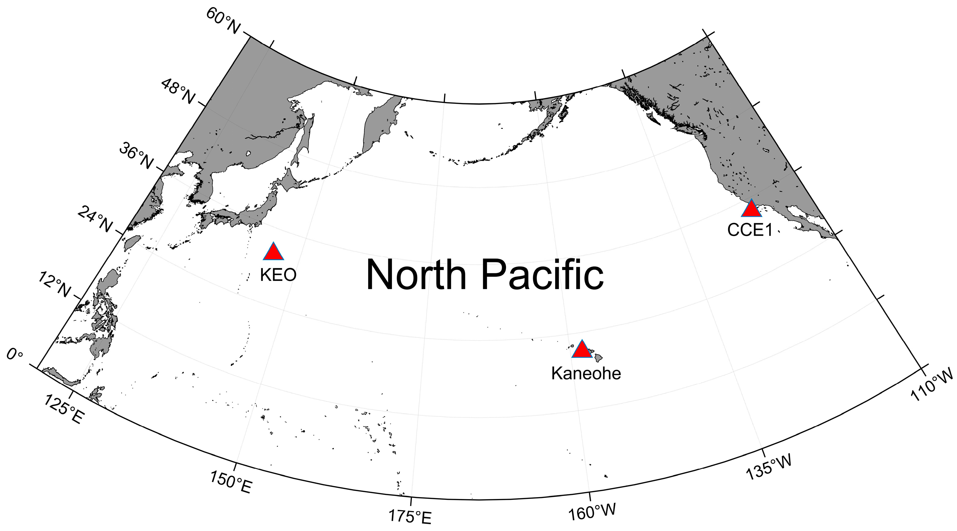
2.1. Data Source

In this study, the surface seawater pH, temperature (SST), salinity (SSS), chlorophyll-a concentration (Chl-a), and pressure of carbon dioxide (pCO2) were derived from the Copernicus Marine Service (CMEMS, https://marine.copernicus.eu/). The accuracy evaluation of each parameter is shown in Table 1 [32,33], and the resolution was 0.25° × 0.25°. The predicted values were highly consistent with Argo data, which can quantify large- and seasonal-scale deviations. At present, these data are widely applied in ocean acidification research [34,35]. Since this data product considers various marine physical and chemical properties, such as the average sea level, nitrate, phosphate, dissolved oxygen, and phytoplankton, when reconstructing seawater pH, the model (PISCES) used was relatively complex. Linear regression, nonlinear random forest regression, and BP neural network methods were relatively mature. These methods were simpler than the physical model, and the variables required for modeling were less and easier to obtain than the complex physical model. They have the characteristics of fast modeling speed, strong simulation ability, and can accurately predict the pH value of seawater. Therefore, this paper used a linear regression, nonlinear regression random forest, and BP neural network algorithm to reconstruct surface seawater pH. We selected the North Pacific (0° N−60° N, 119° E−110° W) as our research area and collected monthly average data from 1993 to 2018 for 76,000 groups. After establishing the surface seawater pH model, which was developed using 50% of the data set, the model was validated on a global and seasonal scale. To verify the reconstruction ability of the model in the North Pacific, we also collected observational data from three time series stations operated by the National Centers for Environmental Information (NCEI): KEO (2001–2002, 2005–2015), CCE1 (2001–2010, 2013–2014), and Kaneohe (2001–2006, 2013–2016) (Figure 1).

2.2. Methods

Three main analytical methods were used: traditional linear regression, nonlinear random forest regression, and the BP neural network algorithm. Traditional linear regression analysis is a statistical technique used to investigate the linear relationship between a continuous dependent variable and one or more independent variables [36]. This method can effectively predict dependent variables. Generally, the correlation coefficient (r) is used to indicate the correlation between variables, while the coefficient of determination (R2) is used to ascertain the fitting effect of the model. The linear regression equation is:
Y = β0 + β1 × 1 + β2X2 + β3X1X2 + ε
In the above equation, Y represents the dependent variable, X1 and X2 represent the independent variables, β0 is the constant term, β1 and β2 are the coefficients for X1 and X2, respectively, β3 is the coefficient for the interaction term between X1 and X2, and ε is the error term.
Random forest is a set of decision trees. Its basic idea is to improve the prediction accuracy of the model by a large number of classification tree sets. The prediction process is shown in Figure 2. As a statistical learning theory, the random forest model needs to determine the two important parameters of mtry and ntree. In order to make the model prediction better, this study set mtry and ntree to 2 and 500.
The BP neural network is a multi-layer feed-forward neural network based on error backpropagation. Through repeated learning of the training samples, the connection weights and thresholds between layers can be continuously adjusted [37], resulting in input information that is similar to the desired output information. The structure of the BP neural network is shown in Figure 3, including the input layer (SST, SSS, Chl-a, and pCO2), the output layer (pH), and the hidden layer.

3. Results

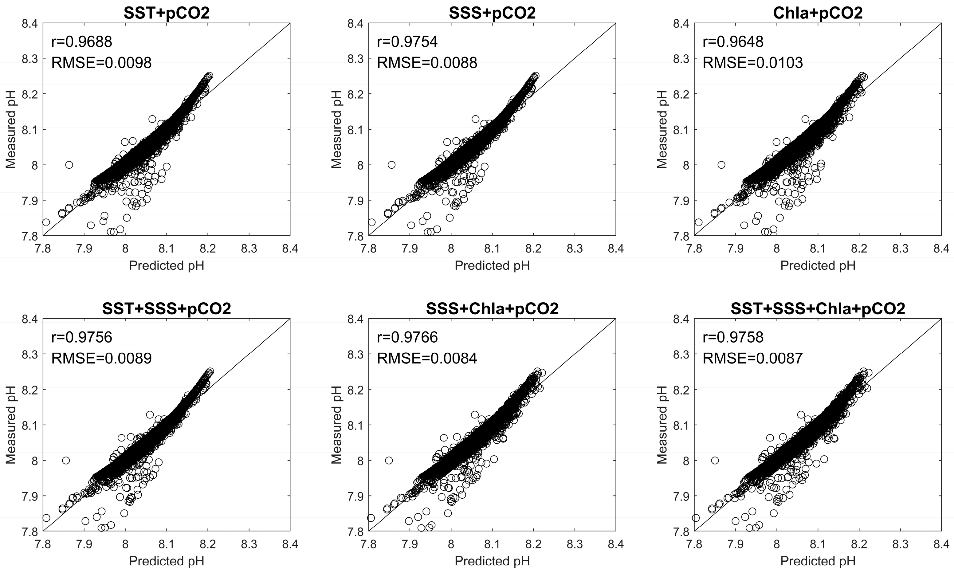
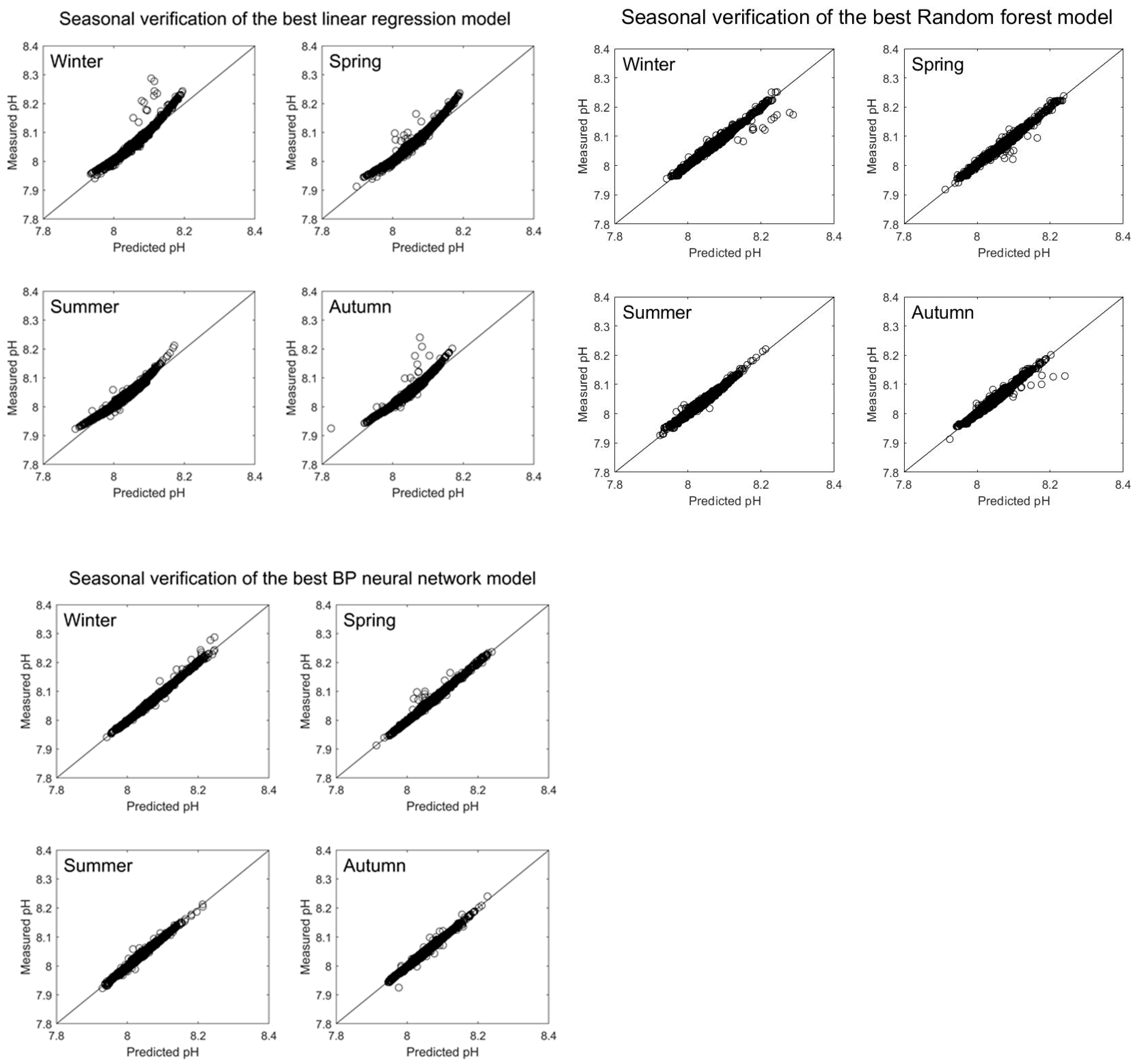
3.1. Establishment and Validation of the Linear Regression Model

The linear regression between SST, SSS, Chl-a, pCO2, the combination of various parameters, and surface seawater pH was analyzed using least-squares. We obtained six linear equations with a determination coefficient (R2) greater than 0.95 (Table 2). The findings demonstrated that the root mean square error (RMSE), standard deviation (Standard), and variance (VAR) of the six linear equations in the model validation were all less than 0.11 and 0.0086, respectively, and there was little difference in each combination. Therefore, it was feasible to reconstruct the surface seawater pH in the North Pacific. The seawater pH model using only SSS, Chl-a, and pCO2 had a comparatively high determination coefficient of 0.9590, while the model using SST, SSS, Chl-a, and pCO2 had a coefficient of 0.9594. However, during model validation, it was discovered that the RMSE, standard, and VAR of the aforementioned parameter combination were the smallest among all six models.
In addition, the predicted and measured values of the validation data analysis model are shown in Figure 4. The predicted values of the six surface seawater pH models based on the traditional linear regression method were relatively close to the measured values. Among the six models, the correlation coefficient of the model based on SSS, Chl-a, and pCO2 had the highest, at 0.9766, and the best-fitting effect. A thorough analysis revealed that the best linear regression model was 8.3096 + 0.0031SSS + 0.0126Chl a − 0.000988pCO2.

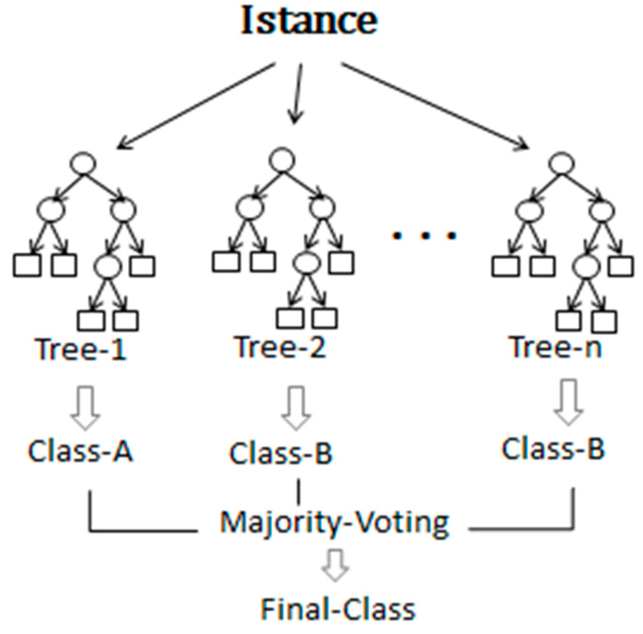
3.2. Establishment and Validation of the Random Forest Model

In the process of random forest modeling, the same 36,000 groups of data were still used as training data, and 20,000 groups of data were used as testing data, making the training data and testing data completely independent. We obtained six different parameter combination models with a determination coefficient greater than 0.95 through modeling, as shown in Table 3. It was found that the RMSE of each parameter combination was less than 0.0085, and the correlation coefficient (r) was greater than 0.97. Among them, the RMSE and r of the seawater pH model based on SST, pCO2, and the combination of SST, SSS, Chl-a, and pCO2 were higher, and the root mean square error was smaller, which was 0.0077.
It can be seen from the model verification of random forest in Figure 5 that the prediction results of each parameter combination were not much different from the real values, and all had good fitting effects. The model based on SST and pCO2 had the best fitting effect, and the correlation coefficient was 0.9808, which was the best random forest regression model for reconstructing the pH value of the surface seawater in the North Pacific.

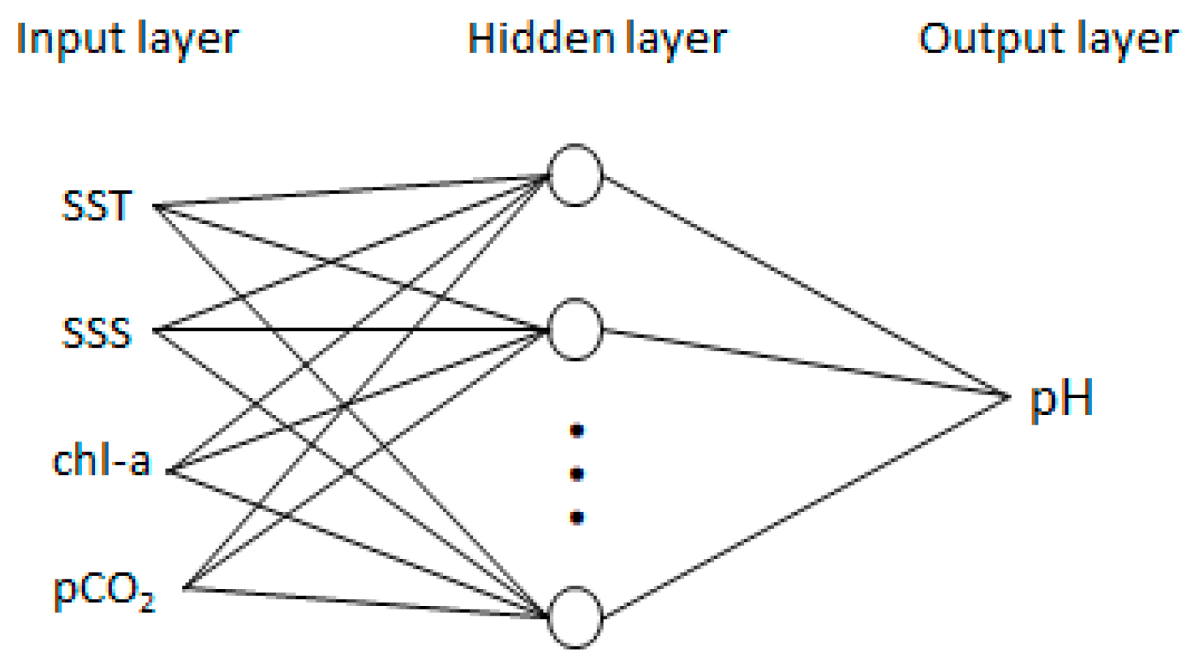
3.3. Establishment and Validation of the BP Neural Network Model

Training mode files were generated using the same 36,000 groups of data as those used in the linear regression modeling, and 20,000 groups of data were used to create test mode files. We obtained six BP neural network models with a determination coefficient greater than 0.95 by using the different selected modeling parameters and combinations as the neurons of the input layer for model training and calculation. Table 4 shows that the RMSE of each parameter combination was less than 0.015, and the correlation coefficient (r) was greater than 0.97. The BP neural network model established using SST, SSS, Chl-a, and pCO2 had the largest determination coefficient and correlation coefficient of the training results and test data and the smallest RMSE value among them.
It is evident from the validation of the model depicted in Figure 6 that the difference between the predicted pH and that the measured pH is minimal. The correlation coefficient of the reconstruction model based on SST, SSS, Chl-a, and pCO2 was 0.9850, indicating that the prediction results highly correlated with the measured values and the model fitting effect was the best. It is clearly the best BP neural network model to reconstruct surface seawater pH in the North Pacific.

3.4. Comparison of Linear Regression, Random Forest, and BP Neural Network Models

The determination coefficient of the best linear regression model was 0.9590, the root mean square error between the model’s predicted values and the measured values was 0.0084, and the correlation coefficient was 0.9766 by comparing the three best models. The determination coefficient of the best random forest model was 0.9571, the root mean square error between the model’s predicted values and the measured values was 0.0077, and the correlation coefficient was 0.9808 by comparing the three best models. Furthermore, the determination coefficient of the best BP neural network model was 0.9702, the RMSE of the model-predicted and measured values was 0.0074, and the correlation coefficient was 0.9850. The best BP neural network model outperformed the best linear regression model and the best random forest model on all evaluation indices.
To compare the best models established by three different methods, this study selected 20,000 groups of data (5000 groups in each season: spring, summer, autumn, and winter) that were not involved in modeling and verification. This was carried out to evaluate the seasonal applicability of surface seawater pH in the North Pacific. According to the fitting degree between the predicted and measured values of the best linear regression model, the best random forest model, and the best BP neural network model in different seasons (Figure 7), it was clear that the best linear regression model had a better fitting effect in summer and autumn, but that effect was rather low in spring and winter. The best random forest model was better than winter and autumn in spring and summer. The best BP neural network model fitted well in spring, summer, autumn, and winter.
In addition, Table 5 shows that the RMSE, standard deviation, and variance of the best linear regression model in the North Pacific in summer were small, at 0.0067, 0.0063, and 0.000039, respectively, while the same values for winter were 0.0097, 0.0093, and 0.000086, respectively. This suggests that the best linear regression model had the best applicability in summer and the worst applicability in winter. The root mean square error, standard deviation, and variance of the best random forest regression model in summer were less than those in spring, autumn, and winter, which were 0.0046, 0.0046, and 0.000021, respectively. This indicates that the applicability of the best random forest regression model in summer was better than that in other seasons. The best BP neural network model had strong applicability in all four seasons, as evidenced by the similar values for the root mean square error, standard deviation, and variance in spring, summer, autumn, and winter. These values were also significantly lower than those for the best linear regression model and the best random forest. A comprehensive comparison revealed that the applicability of the best BP neural network model in spring, summer, autumn, and winter in the North Pacific was generally higher than that of the best linear regression and the best random forest model.

4. Discussion

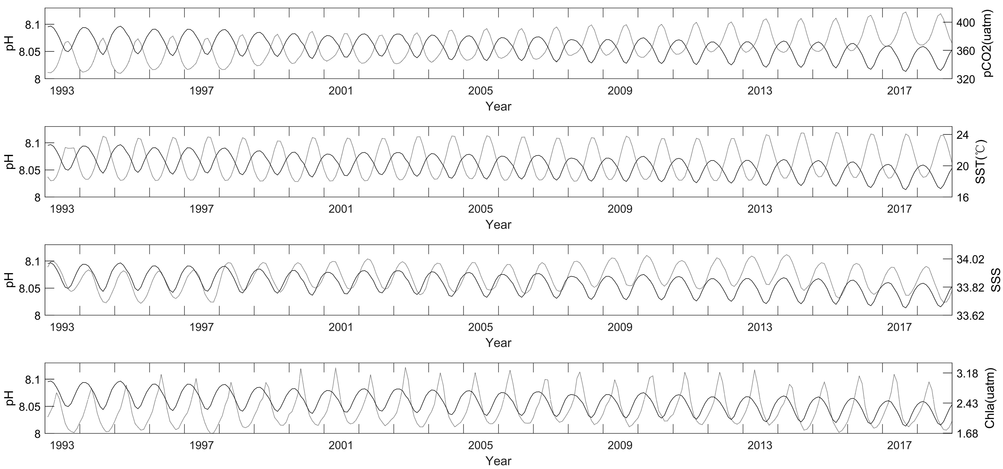
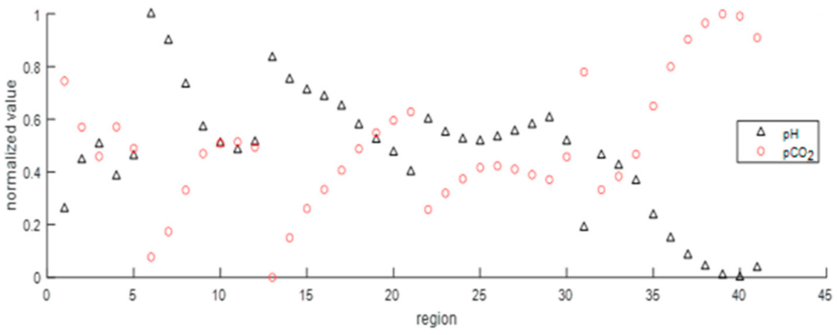
4.1. Effect Mechanism of Seawater pH

In addition to the influence of CO2 on seawater pH, environmental factors, such as temperature, salinity, productivity, nutrient concentration, upwelling, ENSO, and the input of coastal water, could all play a role in ocean acidification [38]. Therefore, this study selected SST, SSS, Chl-a, pCO2, and other parameters as the model’s inputs. According to the monthly variation curves of pH, pCO2, SST, SSS, and Chl-a (Figure 8), it was observed that seawater pH was negatively correlated with pCO2 and SST, and positively correlated with SSS and Chl-a, which was consistent with previous research on the topic. The higher the pCO2 concentration, the lower the seawater pH, indicating that anthropogenic CO2 (the gas exchange process at the air–sea interface) absorbed by the ocean is an important factor affecting the acidification of surface seawater [39,40,41]. The dissolution of CO2, the equilibrium of precipitation and dissolution of CaCO3, the transformation of carbonate minerals, photosynthesis, respiration, and other related physical, chemical, and biological processes contribute to the composition of the seawater carbonate system, which, in turn, is affected by changes in seawater temperature. When the temperature increases, the CO2 content and pH of seawater will decrease. The pH will rise as the temperature drops [42,43]. Salinity has a lower impact on seawater pH than temperature, but it is still significant. The change in pH in the Yangtze Estuary positively correlates with salinity [44]. The influence of regional distribution differences on the CO2 exchange process at the sea–atmosphere interface, as an essential component altering the chemical equilibrium of carbonates, may also contribute to a positive correlation between salinity and pH [45,46]. The Chl-a concentration represents the existing amount of phytoplankton, indicating the ability of marine phytoplankton to convert atmospheric CO2 and bring it into the ocean. When analyzing the factors controlling acidification in the Amundsen Sea and the Ross Sea, Mattsdotter et al. (2011) found that Chl-a had the greatest impact on acidification, while biological factors were the key governing factors for marine acidification in the marginal sea [47]. In addition, researchers analyzed monitoring data from spring in the East China Sea, autumn in the Bohai, and winter in the Yellow Sea, and the results demonstrated a substantial positive correlation between pH and Chl-a [48,49].
In order to quantitatively reveal the relationship between pH and pCO2, this paper also added a geodetector model, which is a statistical method used to detect spatial differentiation characteristics and reveal potential driving forces. It is widely used in ecological environment assessment, natural disaster assessment, and other fields. This method uses q value for quantitative evaluation. The value range is between 0 and 1. The closer q is to 1, the stronger the contribution of the factor to the variable, the closer the correlation between pH and pCO2. This method can be used to more intuitively show the contribution of pCO2 to pH [50]. Considering the large area of the North Pacific, there will be some differences between the sea areas. Therefore, the North Pacific was divided into 50 partitions according to 12° × 12.5°, and the larger land area was removed. Finally, 41 partitions were retained. From the contribution of pCO2 to pH in Figure 9, it can be seen that the contribution of pCO2 to pH in the entire North Pacific was above 0.7, indicating that pCO2 had a greater contribution to pH and the degree of influence was greater. Through the normalization analysis of pCO2 and pH, it was found that for every 10 μatm increase in pCO2, pH decreased by 0.0070–0.0107, as seen in Figure 10.

4.2. Model Evaluation

4.2.1. Comparisons with Previous Research

This paper chose the same time period for investigation as prior studies to verify the reconstruction ability of the model in the North Pacific. As shown in Figure 11, the surface seawater pH in the North Pacific ranged from 7.8 to 8.3 in 2016, with an annual average of 8.0392. Overall, the North Pacific surface seawater pH distribution showed a high trend in the northwest and low in the southeast due to the high productivity induced by rich nutrients and plankton in the northwest. This was because of the influence of complicated circulation, monsoon, land source transport, atmospheric deposition, and seabed sediments [51]. The highest values appeared in the range of 36° N–48° N and 130° W–175° W, especially near the sea areas of China and Japan. This result was consistent with the findings of Jiang et al. (2019), who estimated the pH distribution in the central and northern Pacific regions at in situ temperatures based on SOCATv6 and GLODAPv2 [52].
In this paper, the best BP neural network model was applied to reconstruct surface seawater pH in the North Pacific in February and August 2005. It was found that the surface seawater pH in the North Pacific exhibited apparent seasonal variations. The pH was generally higher in winter than in summer, especially at 24° N–36° N. In February, the pH in the North Pacific was higher in the range of 20° N–48° N, and it was higher in the West than in the East. In August, the pH was higher in the northern and southern parts of the North Pacific than in the central parts, with the northern part having the highest pH Figure 12a,b. This result was similar to the pH distribution of global surface water estimated by Takahashi et al. (2014) in Figure 12c,d, which was based on the pCO2, alkalinity, and nutrient salt concentration data in the GLODAP, CARINA, and LDEO databases in February and August 2005 [53]. This result also suggests that it is feasible to reconstruct the pH in the North Pacific based on the BP neural network model established using SST, SSS, Chl-a, and pCO2 parameters.

4.2.2. Comparison with Copernican Data

Figure 13 shows the difference between the pH reconstructed by the best BP neural network model and that obtained by the Copernicus European Observation Program. In this study, the pH error between the optimal model established by the BP neural network algorithm and the global marine biochemical products was between 0 and 0.02. The areas with significant pH differences between the two occurred in coastal waters, which may be the result of complex physical, chemical, and biological processes in these waters. In addition to sea surface temperature, salinity, and productivity, other factors such as nutrient concentration, upwelling, ENSO, and coastal water inputs were addressed during modelling [38]. However, the model established in this paper was not comprehensive enough to consider the modeling parameters—in comparison to the physical model established by Wooton et al. (2008), which was based on a variety of marine physical characteristics, such as the average sea level, photosynthesis, temperature, upwelling, phytoplankton abundance, and salinity [13]. This model required fewer parameters and was easy to use. The method was relatively simple and could accurately analyze the seasonal characteristics and overall trend of surface seawater pH in the North Pacific.

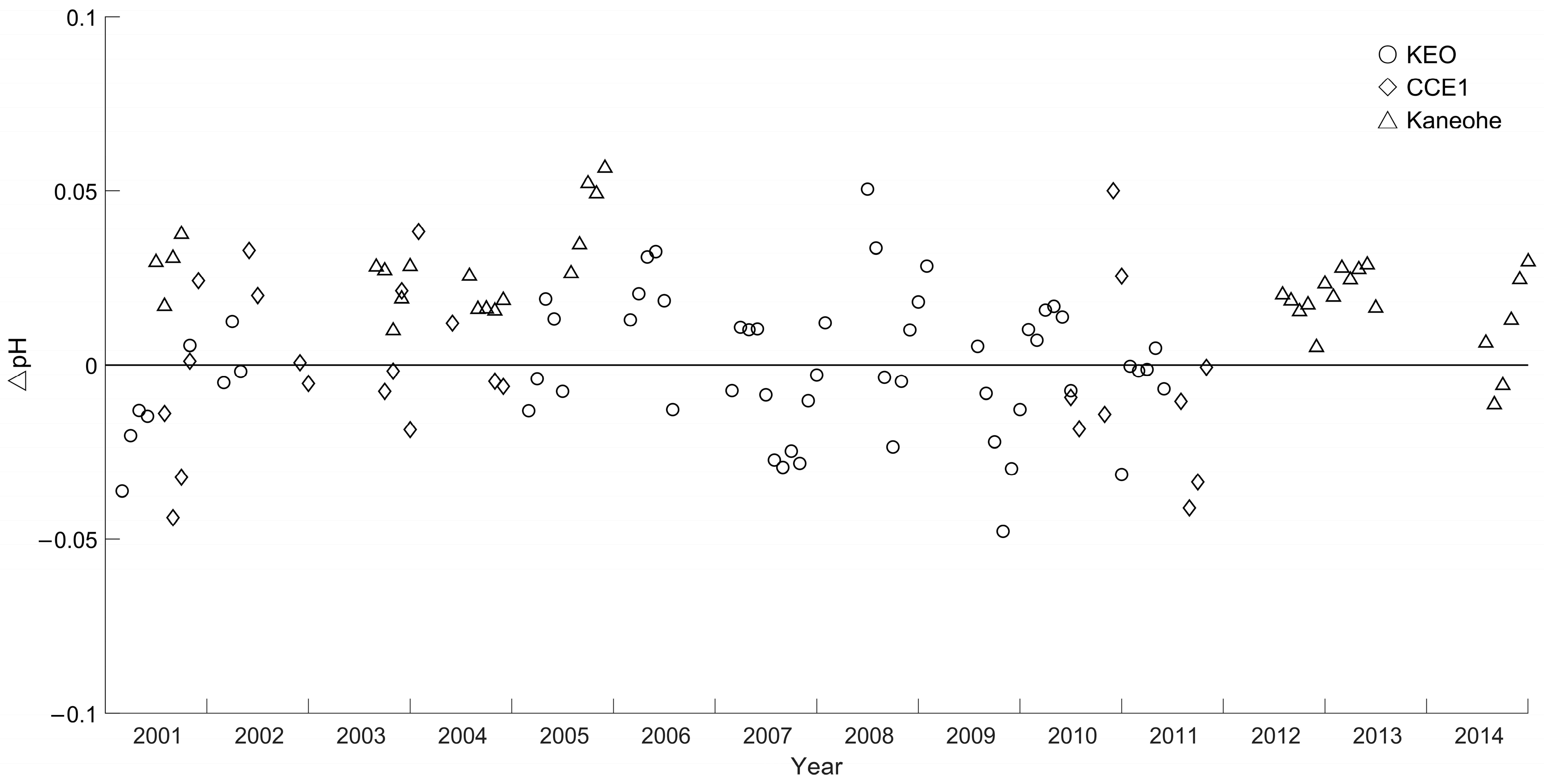
4.2.3. Difference between the Measured and Predicted pH Values

To verify the reliability of the best BP neural network model, we compared the predicted and measured values of three observational time series stations: the KEO in the Northwest Pacific, the CCE1 along the coast of California, and the Kaneohe coral reef station. The average ∆pH (pHpre − pHmea, n = 57) was −0.0008 ± 0.0195 pH in KEO, the average ∆pH (pHpre − pHmea, n = 26) was −0.0014 ± 0.0240 pH in CCE1, and the average ∆pH (pHpre − pHmea, n = 37) was 0.0226 ± 0.0135 pH in Kaneohe (Figure 14). It is clear that the ∆pH of KEO was the smallest, followed by CCE1 and Kaneohe, which was mainly due to the shallow thermocline of CCE1 and the forcing of stable wind [54]. The pH fluctuation of Kaneohe was mainly caused by the influence of the regional marine climate on the exchange of coral reef seawater and open-ocean seawater [55]. The ∆pH in Hawaii was 0.012 ± 0.025, while it was 0.026 ± 0.032 in the Northwest Pacific. Nakano et al. (2005) and Bofeng et al. (2016) found that the ∆pH was 0.017 ± 0.020 pH in the Northwest Pacific when they studied the spatiotemporal distribution of pH in the Arctic sub-polar region based on parametric technology, which was in good agreement with the results of the model reconstruction in this paper [19,22].

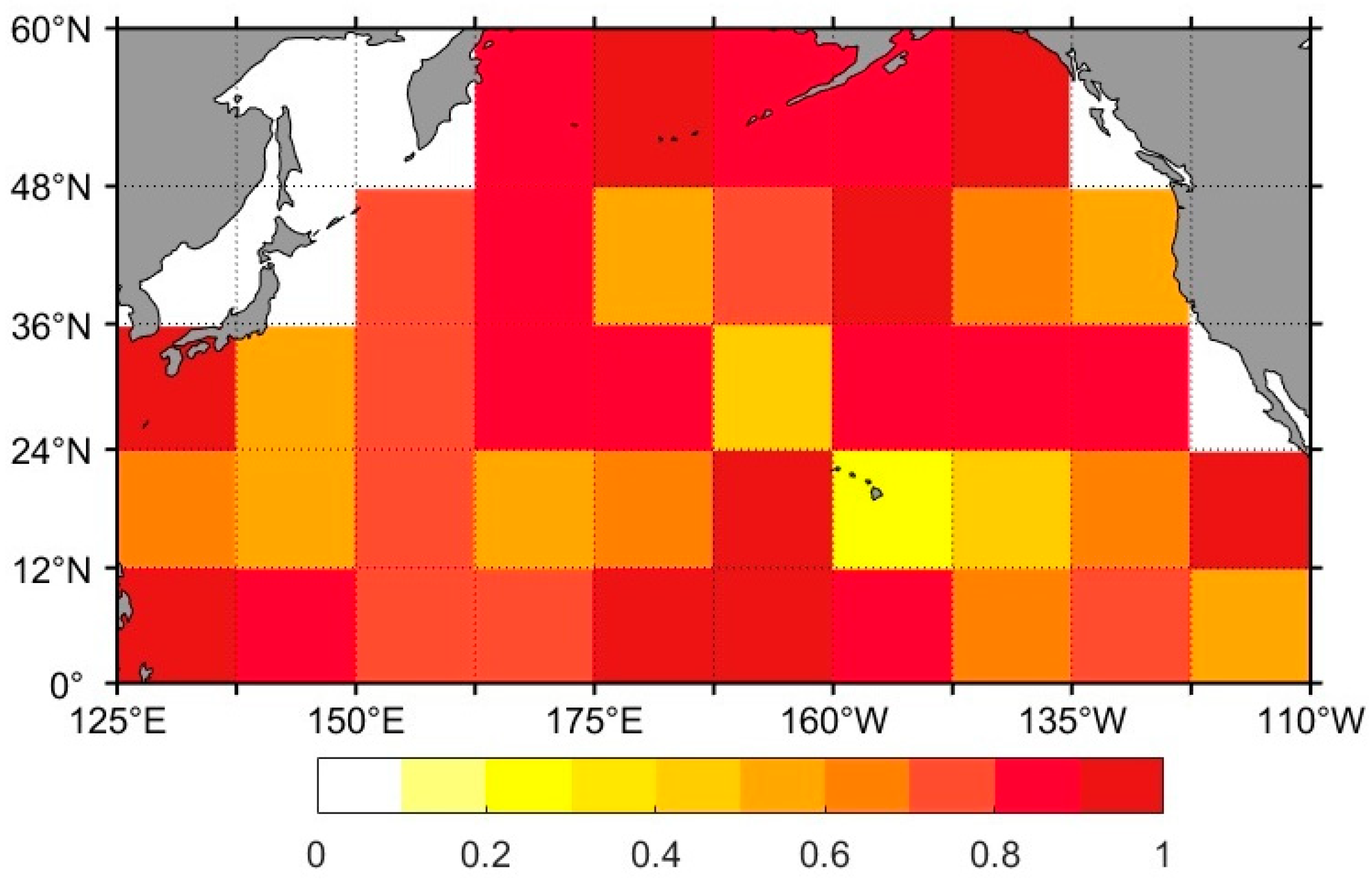
4.3. Application of the Model

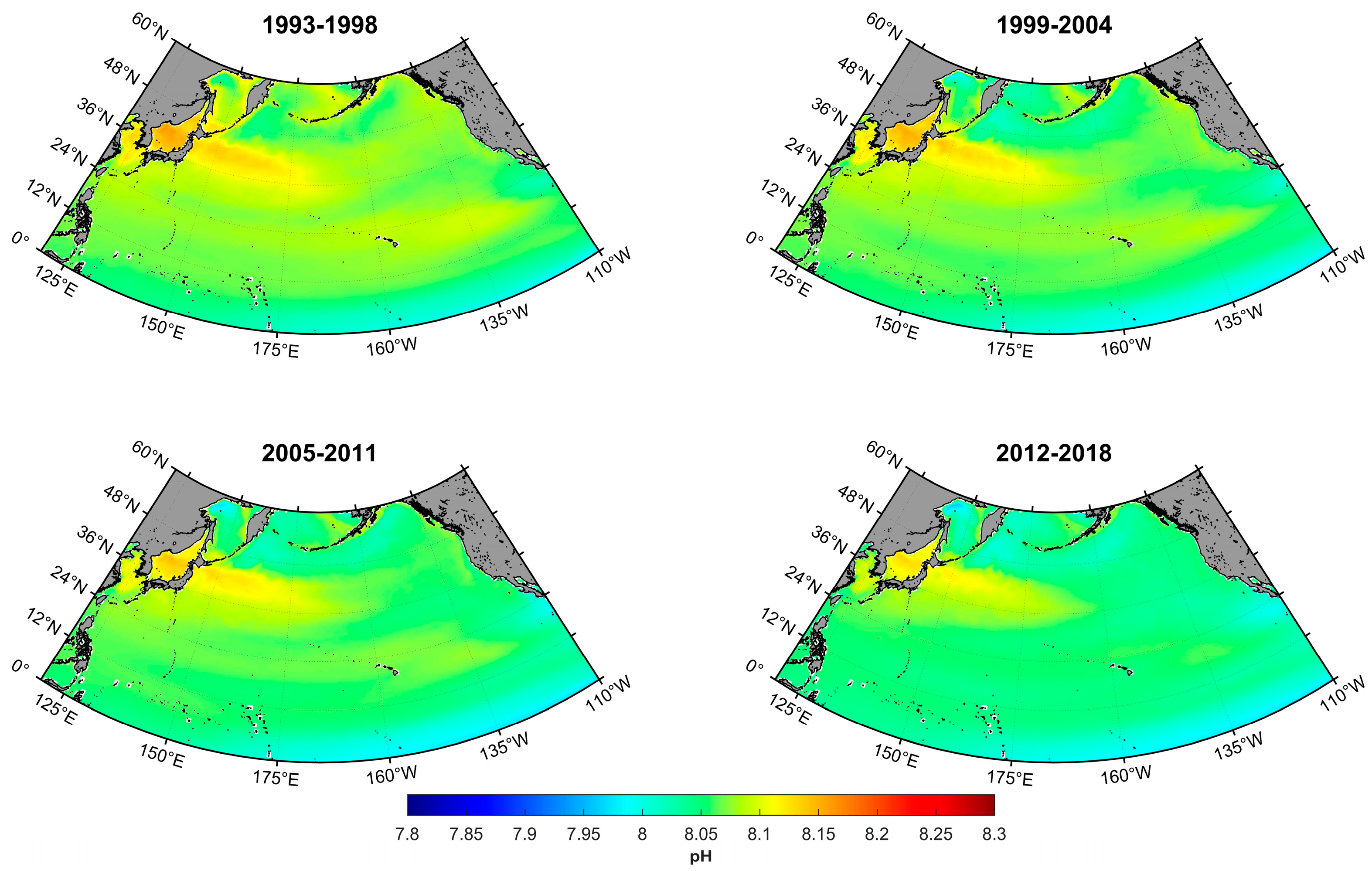
4.3.1. Annual Variability

In the past 26 years, the surface seawater pH in the North Pacific decreased from 8.0749 to 8.0402, with a decline rate of 0.0013 yr −1 (Figure 15). This phenomenon is remarkably similar to the research results of Midorikawa, Dore, Haugan, and Jiang. For example, Midorikawa et al. (2012) found that the decline rate of surface seawater pH was 0.0013 ± 0.0005 yr−1 in summer, and in winter, it was 0.0018 ± 0.0002 yr−1 in the 25-year time series estimation of carbonate parameters in the North Pacific. Dore et al. (2009) showed that the surface seawater pH of the Pacific decreased with a trend of 0.0019 ± 0.002 yr−1 from 1998 to 2007 [56]. Haugan et al. (1996) also showed that pH changes decreased by 0.0015 units per year due to anthropogenic CO2 emissions absorbed by the ocean [7]. Jiang et al. (2019) found that the decrease in pH observed at several open ocean time series stations was 0.0018 yr−1 [51].
Through a surface seawater pH analysis in the North Pacific during 1993–1998, 1999–2004, 2005–2011, and 2012–2018 (Figure 16), apparently the pH was found to be declining; that is, the surface seawater in the North Pacific is continuously experiencing acidification. Over the years, significant spatial differences were observed in the surface seawater pH, exhibiting a general decreasing trend from the northwest to the southeast. The highest value appeared in the tropical western Pacific, with a pH of about 8.2183–8.1820. The lowest value appeared in the eastern equatorial Pacific with upwelling, with a pH of 7.9491–7.9600. Gradually, the tropical western Pacific, located in the southern mainstream of Kuroshio Extension, attained the strongest interannual variation and the highest acidification degree, followed by 24° N–36° N, near the Central Pacific. The eastern equatorial Pacific had the smallest value, and its degree of acidification was not significant [57].

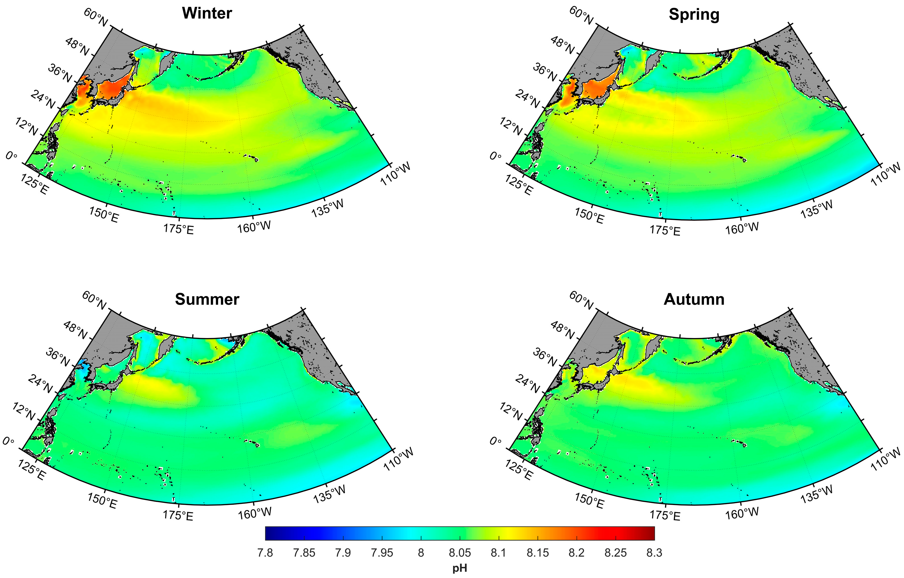
4.3.2. Seasonal Variations

The surface seawater pH in the North Pacific exhibited aboriginal and stable seasonal characteristics. The overall pH was as follows: pHwinter > pHspring > pHautumn > pHsummer (Figure 17). In winter, the SST was low, and the pH was higher than in other seasons. The pH was high at 24° N–48° N. Additionally, it was higher in the West than in the East. In spring, with an increase in SST, phytoplankton begins to grow, and the chlorophyll concentration reaches a maximum; however, it is less than that in winter. The pH exhibited a downward trend, and the distribution characteristics were similar to those in winter. In autumn, the SST decreases, and the pH increases in a wide range; its distribution characteristics are similar to those in winter. Overall, the north and south sides have higher values than the central sea area, and the pH on the north side is the highest. In summer, due to the high SST, the upper water mass is stable, the vertical mixing is weak, and the large volume of phytoplankton in spring consumes part of the surface carbon. The pH in most of the sea area reaches a minimum value, and the higher values are basically distributed along the coast. The pH value of surface seawater in summer is much lower than that in winter, which is mainly affected by sea surface temperature. The sea surface temperature is negatively correlated with the pH value. The seawater pH in winter is higher than that in summer because of the sea surface temperature in summer is higher than that in winter. For example, the studies of González-Dávila [42], Raven [43], Nakano [19], Shi Qiang [21], and others confirmed that the pH value decreased when the sea surface temperature increased. In addition, Midorikawa et al.‘s research on the Northwest Pacific Ocean showed that the contribution rate of seawater temperature rise to the decrease in pH value was about 15% [11].
According to the seasonal differences in surface seawater pH in the North Pacific between 1993 and 2018 (Figure 18), the pH changes in most of the North Pacific were negative, indicating that the pH was in decline since 1993. From the seasonal variation range of pH over many years, the acidification degrees of different sea areas in the four seasons differ. The pH variation value near the East Equator was near or above 0, indicating that the acidification degree was weak, and the pH fluctuation range of the coastal areas was larger than that in other sea areas, indicating that the introduction of land sources accelerated ocean acidification [15]. The pH changes in the near-eastern equatorial region were the smallest in summer, autumn, and winter, and increased in spring, summer, and autumn near 40° N–44° N and 150° E–175° E.

5. Summary and Conclusions

In this study, the physical and chemical parameters related to surface seawater pH were used as modeling parameters to compare the reconstruction ability of traditional linear regression, nonlinear regression random forest, and BP neural network algorithms in the North Pacific, and the spatiotemporal distribution characteristics were analyzed using the best model.
Three methods had good reconstruction ability for surface seawater pH in the North Pacific. The linear regression model had the best simulation accuracy based on SST, Chl-a, and pCO2; the random forest regression model had the best simulation accuracy based on SST and pCO2; and the BP neural network model had the best simulation accuracy based on SST, SSS, Chl-a, and pCO2.
Comparing the RMSE and fitting coefficients of the three best models, it was evident that the BP neural network model was better than the linear regression model and random forest model, with strong applicability in spring, summer, autumn, and winter.
The pH was affected by many environmental factors; it was negatively correlated with pCO2 and SST, positively correlated with SSS and Chl-a, and primarily affected by the CO2 exchange process at the sea–air interface. In addition, the application of the best model in this study found that sea surface pH exhibited obvious interannual and seasonal variations. Over the past 26 years, the pH in the North Pacific was decreasing at a rate of 0.0013 yr−1, with a distribution trend of high in the northwest and low in the southeast. The pH in winter was higher than that in summer; in winter, it was higher at 20° N–48° N and higher in the West than in the East. In summer, the northern and southern sea areas had higher values than the central sea areas, with the northern sea area having the highest value.
The model established in this paper was consistent with existing studies in terms of both seasonal and spatial distributions. However, due to the influence of complex physical, chemical, and biological processes, the reconstruction error of seawater pH in coastal waters was large. In addition to considering the temperature, salinity, and productivity used in this study, the effects of nutrient concentration, upwelling, ENSO, and other factors in modeling should be researched in the future.

Author Contributions

Conceptualization, J.W. (Jie Wang) and J.M.; data curation, P.Y. and J.W. (Jiarui Wang); formal analysis, J.X.; investigation, J.W. (Jiarui Wang); methodology, J.L.; resources, P.Y.; software, J.L.; validation, J.X.; writing—original draft, J.W. (Jie Wang) and X.W.; writing—review and editing, J.M. All authors have read and agreed to the published version of the manuscript.

Funding

This research received no external funding.

Institutional Review Board Statement

This research did not require ethical approval.

Informed Consent Statement

This research not involving humans.

Data Availability Statement

The data that support the findings of this study are available in the Copernicus Marine Service (CMEMS). These data were derived from the following resources available in the public domain: https://marine.copernicus.eu/.

Acknowledgments

We extend a special thanks to the Copernicus Marine Service (CMEMS) and the National Centers for Environmental Information (NCEI) for providing data for this study. We also thank the many scientists and technicians for their assistance with the collection of hydrographic data in the North Pacific and their dedicated work during the long-term observations. We thank Taro Takahashi et al. for the use of the pH distribution of global surface.

Conflicts of Interest

The authors declare that they have no known competing financial interests or personal relationships that could have appeared to influence the work reported in this paper. This research did not receive any specific grant from funding agencies in the public, commercial, or not-for-profit sectors.

References

  1. Yu, W.Y.; Zhang, C.Y.; Feng, Z.G.; Guo, L. Global ocean acidification research trend and latest progress analysis. Mar. Sci. J. 2016, 2016, 296–307. [Google Scholar]
  2. Orr, J.; Fabry, V.; Aumont, O.; Bopp, L.; Doney, C.; Feely, A.; Gnanadesikan, A.; Gruber, N.; Ishida, A.; Joos, F.; et al. Anthropogenic ocean acidification over the twenty-first century and its impact on calcifying organisms. Nature 2005, 437, 681–686. [Google Scholar] [CrossRef] [PubMed] [Green Version]
  3. Richard, F.; Scott, D.; Sarah, C. Ocean Acidification: Present Conditions and Future Changes in a High-CO2 World. Oceanography 2009, 22, 36–47. [Google Scholar]
  4. He, S.C.; Zhang, Y.H.; Chen, L.Q.; Li, W. Marine acidification research progress. Mar. Sci. 2014, 38, 85–93. [Google Scholar]
  5. Watanabe, Y.W.; Li, F.; Yamasaki, R.; Yunoki, S.; Lmai, K.; Hosoda, S.; Nakano, Y. Spatiotemporal changes of ocean carbon species in the western North Pacific using parameterization technique. J. Oceanogr. 2020, 76, 155–167. [Google Scholar] [CrossRef]
  6. Caldeira, K.; Wickett. Oceanography: Anthropogenic carbon ocean pH. Nature 2003, 425, 365. [Google Scholar] [CrossRef] [Green Version]
  7. Haugan, P.M.; Drange, H. Effects of CO2 on the ocean environment. Energy Convers. Manag. 1996, 37, 1019–1022. [Google Scholar] [CrossRef]
  8. Bates, N.R.; Astor, Y.M.; Church, M.; Currie, K.; Dore, E. A time-series view of changing surface ocean chemistry due to ocean uptake of anthropogenic CO2 and ocean acidification. Oceanography. 2014, 27, 126–141. [Google Scholar] [CrossRef] [Green Version]
  9. Doney, S.C.; Fabry, V.J.; Feely, R.A. Ocean acidification: The other CO2 problem. Annu. Rev. Mar. Sci. 2009, 1, 169–192. [Google Scholar] [CrossRef] [PubMed] [Green Version]
  10. Feely, R.A.; Fabry, V.J.; Guinotte, J.M. Ocean acidification of the North Pacific Ocean. PICES Press 2008, 16, 22–26. [Google Scholar]
  11. Midorikawa, T.; Inoue, H.Y.; Ishii, M.; Sasano, D.; Kosugi, N.; Hashida, G.; Nakaoka, S.; Suzuki, T. Decreasing pH trend estimated from 35-year time series of carbonate parameters in the Pacific sector of the Southern Ocean in summer. Deep Sea Res. Part I Oceanogr. Res. Pap. 2012, 61, 131–139. [Google Scholar] [CrossRef]
  12. Polonsky, A. Had been observing the acidification of the black sea upper layer in XX Century. Turk. J. Fish. Aquat. Sci. 2012, 12, 391–396. [Google Scholar] [CrossRef] [PubMed]
  13. Wootton, J.T.; Pfister, C.A.; Forester, J.D. Dynamic patterns and ecological impacts of declining ocean pH in a high-resolution multi-year dataset. Proc. Natl. Acad. Sci. USA 2008, 105, 18848–18853. [Google Scholar] [CrossRef] [Green Version]
  14. Byrne, R.H.; Mecking, S.; Feely, R.A.; Liu, X.W. Direct observations of basin-wide acidification of the North Pacific Ocean. Geophys. Res. Lett. 2010, 37, L02601. [Google Scholar] [CrossRef] [Green Version]
  15. Cai, W.J.; Hu, X.P.; Huang, W.J.; Murrell, C.; Lehrter, C.; Lohrenz, E.; Chou, W.C.; Zhai, W.D.; Hollibaugh, T.; Wang, Y.C.; et al. Acidification of subsurface coastal waters enhanced by eutrophication. Nat. Geosci. 2011, 4, 766–770. [Google Scholar] [CrossRef]
  16. Dickson, A.G. The measurement of sea water pH. Mar. Chem. 1993, 44, 131–142. [Google Scholar] [CrossRef]
  17. Feely, R.A.; Sabine, C.L.; Lee, K.; Berelson, W.; Kleypas, J.; Fabry, J.; Millero, J. Impact of anthropogenic CO2 on the CaCO3 system in the oceans. Science 2004, 305, 362–366. [Google Scholar] [CrossRef] [Green Version]
  18. Li, F.R. Distribution characteristics and influencing factors of seawater pH in the adjacent sea area of the Yellow River estuary in August 1985. Mar. Lake Marsh Notif. 1998, 4, 35–40. [Google Scholar]
  19. Nakano, Y.; Watanabe, Y.W. Reconstruction of pH in the surface seawater over the North Pacific basin for all seasons using temperature and chlorophyll-a. J. Oceanogr. 2005, 61, 673–680. [Google Scholar] [CrossRef]
  20. Alin, S.R.; Feely, R.A.; Dickson, A.G.; Hernández-Ayón, J.; Juranek, W.; Ohman, D.; Goericke, R. Robust empirical relationships for estimating the carbonate system in the southern California Current System and application to CalCOFI hydrographic cruise data (2005–2011). J. Geophys. Res. 2012, 117, C05033-1–C05033-16. [Google Scholar] [CrossRef] [Green Version]
  21. Shi, Q.; Yang, P.J.; Huo, S.X.; Bu, Z.G. Process of Seawater Acidification in Bohai Sea in Recent 36 Years. In Proceedings of the Academic Annual Meeting of the Chinese Society of Environmental Sciences, Chengdu, China, 22–23 October 2013; pp. 114–121. [Google Scholar]
  22. Bofeng, L.; Yutaka. Spatiotemporal distribution of seawater pH in the North Pacific subpolar region by using the parameterization technique. J. Geophys. Res. Oceans. JGR 2016, 121, 3435–3449. [Google Scholar]
  23. Guo, Y.; Yang, X.Q. Temporal and spatial characteristics of interannual and interdecadal variations in the global ocean-atmosphere system. Sci. Meteorol. Sin. 2002, 2, 127–138. [Google Scholar]
  24. Friedrich, T.; Oschlies, A. Neural network-based estimates of north atlantic surface pCO2 from satellite data: A methodological study. J. Geophys. Res. 2009, 114, JC004646. [Google Scholar] [CrossRef] [Green Version]
  25. Laruelle, G.G.; Landschützer, P.; Gruber, N.; Tison, J.; Delille, B.; Regnier, P. Global high-resolution monthly pCO2 climatology for the coastal ocean derived from neural network interpolation. Biogeosciences 2017, 14, 4545–4561. [Google Scholar] [CrossRef] [Green Version]
  26. Bostock, H.C.; Mikaloff Fletcher, S.E.; Williams, M.J.M. Estimating carbonate parameters from hydrographic data for the intermediate and deep waters of the Southern Hemisphere oceans. Biogeosciences 2013, 10, 6199–6213. [Google Scholar] [CrossRef] [Green Version]
  27. Sasse, T.P.; McNeil, B.I.; Abramowitz, G. A novel method for diagnosing seasonal to inter-annual surface ocean carbon dynamics from bottle data using neural networks. Biogeosciences 2013, 10, 4319–4340. [Google Scholar] [CrossRef] [Green Version]
  28. Velo, A.; Pérez, F.F.; Tanhua, T.; Gilcoto, M.; Ríos, A.F.; Key, R.M. Total alkalinity estimation using MLR and neural network techniques. J. Mar. Syst. 2013, 111, 11–18. [Google Scholar] [CrossRef] [Green Version]
  29. Chen, Q.H.; Peng, H.J. Research progress on ecological hazards of ocean acidification. Sci. Technol. Rep. 2009, 27, 108–111. [Google Scholar]
  30. Guo, J.T. Evolution of Surface pH and pCO2 in the Tropical Western Pacific and Its Influencing Factors in 150,000 Years; Graduate School of Chinese Academy of Sciences (Institute of Oceanography): Bejing, China, 2015. [Google Scholar]
  31. Chen, L.T.; Wu, R.G. The combined effects of SST anomalies in the Pacific on the summer rainband types in eastern China. Atmos. Sci. 1998, 5, 43–51. [Google Scholar]
  32. Charles, D.; Gilles, G.; Charly, R. Quality Information Document for Global Ocean Reanalysis Multi-Model Ensemble Products GREP; Copernicus: Brussels, Belgium, 2019. [Google Scholar]
  33. Julien, L.; Coralie, P.; Alexandre, M. Quality Information Document for Global Biogeochemical Analysis and Forecast Product; CMEMS: Ramonville-Saint-Agne, France, 2019. [Google Scholar]
  34. Sridevi, B.; Sarma, V.V.S.S. Role of river discharge and warming on ocean acidification and pCO2 levels in the Bay of Bengal. Tellus B Chem. Phys. Meteorol. 2021, 73, 1–20. [Google Scholar] [CrossRef]
  35. Monaco, C.L.; Metzl, N.; Fin, J.; Mignon, C.; Cuet, P.; Douville, E.; Gehlen, M.; Chau, T.; Tribollet, A. Distribution and long-term change of the sea surface carbonate system in the Mozambique Channel (1963–2019). Deep Sea Res. Part II Top. Stud. Oceanogr. 2021, 1, 104936. [Google Scholar] [CrossRef]
  36. Zhang, J.Y.; Pan, G.Y. Multiple linear regression and BP neural network prediction model comparison and application research. J. Kunming Univ. Technol. Nat. Sci. Ed. 2013, 6, 61–67. [Google Scholar]
  37. Zhang, Y.C.; Qian, X.; Qian, Y.; Liu, J.P.; Kong, F.X. Quantitative remote sensing study of chlorophyll a in Taihu Lake based on machine learning method. Environ. Sci. 2009, 30, 1321–1328. [Google Scholar]
  38. Duarte, C.M.; Hendriks, I.E.; Moore, T.S.; Olsen, S.; Steckbauer, A.; Ramajo, L.; Carstensen, J.; Trotter, A.; McCulloch, M. Is ocean acidification an open-ocean syndrome? Understanding anthropogenic impacts on seawater pH. Estuaries Coasts 2013, 36, 221–236. [Google Scholar] [CrossRef] [Green Version]
  39. Omar, A.M.; Thomas, H.; Olsen, A.; Becker, M.; Skjelvan, I.; Reverdin, G. Trends of Ocean Acidification and pCO2 in the Northern North Sea, 2003–2015. J. Geophys. Res. Biogeosci. 2019, 124, 3088–3103. [Google Scholar] [CrossRef] [Green Version]
  40. Sutton, A.J.; Feely, R.A.; Maenner-Jones, S.; Musielwicz, S.; Osborne, J.; Dietrich, C.; Monacci, N.; Cross, J.; Bott, R.; Kozyr, A. Autonomous seawater pCO2 and pH time series from 40 surface buoys and the emergence of anthropogenic trends. Earth Syst. Sci. Data 2019, 11, 421–439. [Google Scholar] [CrossRef] [Green Version]
  41. Zhang, L.J.; Wang, J.J.; Zhang, Y.; Xue, L. Distribution and influencing factors of pCO2 in surface seawater of the North Yellow Sea in winter. J. Ocean Univ. China Nat. Sci. Ed. 2008, 6, 955–960. [Google Scholar]
  42. González-Dávila, M.; Santana-Casiano, J.M.; Rueda, M.J.; Llinás, O.; González-Dávila, E. Seasonal and interannual variability of sea-surface carbon dioxide species at the European Station for Time Series in the Ocean at the Canary Islands (ESTOC) between 1996 and 2000. Glob. Biogeochem. Cycles 2003, 17, GB001993. [Google Scholar] [CrossRef] [Green Version]
  43. Raven, J.; Caldeira, K.; Elderfield, H.; Hoegh-Guldberg, O.; Liss, P.; Riebesell, U.; Shepherd, J.; Turley, C.; Watson, A. Ocean Acidification Due to Increasing Atmospheric Carbon Dioxide; The Royal Society: London, UK, 2005; pp. 5–13. [Google Scholar]
  44. Liu, X.H.; Sun, D.Q.; Huang, B.; Wang, J.X. Research on the trend and influencing factors of surface seawater acidification in the coastal waters of the East China Sea. Ocean. Lakes 2017, 48, 398–405. [Google Scholar]
  45. Zeebe, R.E. History of seawater carbonate chemistry, atmospheric CO2, and ocean acidification. Annu. Rev. Earth Planet. Sci. 2012, 40, 141–165. [Google Scholar] [CrossRef] [Green Version]
  46. Xiao, Z.L. Study on Ocean Acidification in the Chukchi Sea and the Nordic Sea; Third Marine Research Institute, National Oceanic Administration: Washington, DC, USA, 2015.
  47. Mattsdotter Björk, M.; Fransson, A.; Torstensson, A.; Chierici, M. Ocean acidification state in western Antarctic surface waters: Controls and interannual variability. Biogeosciences 2014, 11, 57–73. [Google Scholar] [CrossRef] [Green Version]
  48. Sun, J.; Liu, D.Y.; Chai, X.Y.; Zhang, C. Estimate of chlorophyll a concentration and primary productivity in central Bohai and its adjacent waters in spring and autumn 1998–1999. Ecology 2003, 3, 517–526. [Google Scholar]
  49. Shi, X.Y.; Wang, X.L.; Lu, R.; Sun, X. Distribution characteristics and influencing factors of dissolved oxygen and pH in spring in red tide high-incidence area of East China Sea. Ocean Lake 2005, 5, 404–412. [Google Scholar]
  50. Wang, J.; Zhu, S.R.; Liu, J.M.; Wang, X.; Wang, J.R.; Xu, J.Y.; Yao, P.L.; Yang, Y.J. Frequency, Intensity and Influences of Tropical Cyclones in the Northwest Pacific and China, 1977–2018. Sustainability 2023, 15, 3933. [Google Scholar] [CrossRef]
  51. Ji, X.L. Numerical Simulation Study on Carbon Cycle of Marine Ecosystems in the Northwest Pacific; National Marine Environment Prediction Research Center: Beijing, China, 2013.
  52. Jiang, L.Q.; Carter, B.R.; Feely, R.A.; Lauvset, K.; Olsen, A. Surface ocean pH and buffer capacity: Past, present and future. Sci. Rep. 2019, 9, 18624. [Google Scholar] [CrossRef] [Green Version]
  53. Takahashi, T.; Sutherland, S.C.; Chipman, D.W.; Goddard, J.G.; Cheng, H.; Newberger, T.; Sweeney, C.; Munro, D.R. Climatological distributions of pH, pCO2, total CO2, alkalinity, and CaCO3 saturation in the global surface ocean, and temporal changes at selected locations. Mar. Chem. 2014, 164, 95–125. [Google Scholar] [CrossRef] [Green Version]
  54. Qu, B.X.; Song, J.J.; Li, X.G. Research progress on time series of ocean acidification. Mar. Notif. 2020, 39, 281–290. [Google Scholar]
  55. Chen, X.F.; Wei, G.J.; Deng, W.F.; Zou, J.Q. Coral reef seawater pH change and its significance for ocean acidification. Trop. Geogr. 2016, 36, 41–47. [Google Scholar]
  56. Dore, E.; Lukas, S.; Sadler, W.; Church, J.; Karl, M. Physical and biogeochemical modulation of ocean acidification in the central North Pacific. Proc. Natl. Acad. Sci. USA 2009, 106, 30. [Google Scholar] [CrossRef] [Green Version]
  57. Pelejero, C.; Calvo, E.; Mcculloch, M.; Marshall, F.; Gagan, K.; Lough, M.; Opdyke, N. Preindustrial to modern interdecadal variability in coral reef pH. Science 2005, 309, 2204–2207. [Google Scholar] [CrossRef]
Figure 1. Open triangles represent the study area, including the time series stations KEO (32° N, 145° E), CCE1 (33° N, 122° W), and Kaneohe (21° N, 158° W).
Sustainability 15 05796 g001
Figure 2. Random forest prediction flow chart.
Sustainability 15 05796 g002
Figure 3. Structure of the BP neural network.
Sustainability 15 05796 g003
Figure 4. Validation of the linear regression model.
Sustainability 15 05796 g004
Figure 5. Validation of the random forest model.
Sustainability 15 05796 g005
Figure 6. Validation of the BP neural network model.
Sustainability 15 05796 g006
Figure 7. Seasonal verification of the linear regression, random forest, and BP neural network models.
Sustainability 15 05796 g007
Figure 8. Monthly variation curves of pH, pCO2, SST, SSS, and Chl-a from 1993 to 2018.
Sustainability 15 05796 g008
Figure 9. The contribution of pCO2 to pH.
Sustainability 15 05796 g009
Figure 10. Relative relationship between pCO2 and pH.
Sustainability 15 05796 g010
Figure 11. pH distribution of surface seawater in the North Pacific in 2016.
Sustainability 15 05796 g011
Figure 12. Distribution of pH in the North Pacific in February and August. (a,b) use of the best BP neural networks. (c,d) use of the data from Takahashi et al.’s study (Available online: https://www.ldeo.columbia.edu/res/pi/CO2/, accessed on 25 May 2022).
Sustainability 15 05796 g012
Figure 13. pH difference between the BP model and Copernican products in the surface water of the North Pacific in 2016.
Sustainability 15 05796 g013
Figure 14. Differences in the predicted and measured pH values at KEO, CCE1, and Kaneohe.
Sustainability 15 05796 g014
Figure 15. pH curve in the North Pacific from 1993 to 2018.
Sustainability 15 05796 g015
Figure 16. pH distribution in different years in the North Pacific.
Sustainability 15 05796 g016
Figure 17. Seasonal distribution of surface seawater pH in the North Pacific from 1993 to 2018.
Sustainability 15 05796 g017
Figure 18. Seasonal differences in surface seawater pH in the North Pacific between 1993 and 2018.
Sustainability 15 05796 g018
Table 1. Accuracy evaluation of each parameter and measured data.
RBIASRMSE
SST\\0.76
SSS\\0.22
Chla0.8110.260.59
pH0.9520.020.04
Table 2. Output results of the pH reconstruction model based on linear regression.
Modelling Data (n = 36,000)Verification Data (n = 20,000)
R2Linear EquationRMSEStandardVAR
SST + pCO20.95038.4212 + 0.0001SST − 0.001pCO20.00980.00970.000095
SSS + pCO20.95228.3659 + 0.0017SSS − 0.001pCO20.00880.00870.000075
Chl-a + pCO20.95268.4169 + 0.0071Chla − 0.00099pCO20.01030.01030.000106
SST + SSS + pCO20.95228.3632 − 0.0000238SST + 0.0018SSS − 0.0009997pCO20.00890.00860.008600
SSS + Chl-a + pCO20.95908.3096 + 0.0031SSS + 0.0126Chla − 0.000988pCO20.00840.00840.000071
SST + SSS + Chl-a + pCO20.95948.3197 + 0.000128SST + 0.0028SSS + 0.0136Chla − 0.000992pCO20.00870.00860.000074
Table 3. Random forest model (36,000 groups of data as training data, and 20,000 groups of data as testing data).
R2RMSEr
SST + pCO20.95710.00770.9808
SSS + pCO20.95010.00820.9777
Chl-a + pCO20.95120.00820.9780
SST + Chl-a + pCO20.95540.00780.9800
SSS + Chl-a + pCO20.95160.00810.9786
SST + SSS + Chl-a + pCO20.95640.00770.9806
Table 4. BP neural network model (36,000 groups of data as training data, and 20,000 groups of data as test data).
R2RMSEr
SST + pCO20.96330.00810.9815
SSS + pCO20.95510.01400.9773
Chl-a + pCO20.95380.00900.9766
SST + SSS + pCO20.96820.00770.9839
SSS + Chl-a + pCO20.96910.00770.9844
SST + SSS + Chl-a + pCO20.97020.00740.9850
Table 5. Seasonal verification of the linear regression, random forest, and BP neural network models.
RMSESTDVAR
SeasonnLinearRFBPLinearRFBPLinearRFBP
Winter50000.00970.00580.00470.00930.00580.00340.00008620.00003410.0000116
Spring50000.00820.00510.00490.00770.00500.00370.00005960.00002480.0000138
Summer50000.00670.00460.00420.00630.00460.00330.00003930.00002140.0000109
Autumn50000.00740.00530.00420.00730.00520.00320.00005290.00002750.0000104
Disclaimer/Publisher’s Note: The statements, opinions and data contained in all publications are solely those of the individual author(s) and contributor(s) and not of MDPI and/or the editor(s). MDPI and/or the editor(s) disclaim responsibility for any injury to people or property resulting from any ideas, methods, instructions or products referred to in the content.

