
An Integrated Deep-Learning-Based Approach for Energy Consumption Prediction of Machining Systems


Abstract
:1. Introduction
- A framework for predicting the EC of machining systems based on deep learning is proposed. A particle swarm algorithm is improved using dynamic inertia weights, and then a double-layer LSTM network is introduced to predict the EC of machining systems.
- A novel method for constructing EC datasets is proposed. This method is intended to improve the generalization ability of the prediction model by mixing EC data generated in different ways to produce a novel EC dataset.
- The EC patterns of the machining systems are classified according to the processing characteristics. The processing energy consumption data of different processing characteristics are collected, so as to accurately predict the processing EC.
2. Theoretical Background
2.1. EC Characteristics of Machining Systems
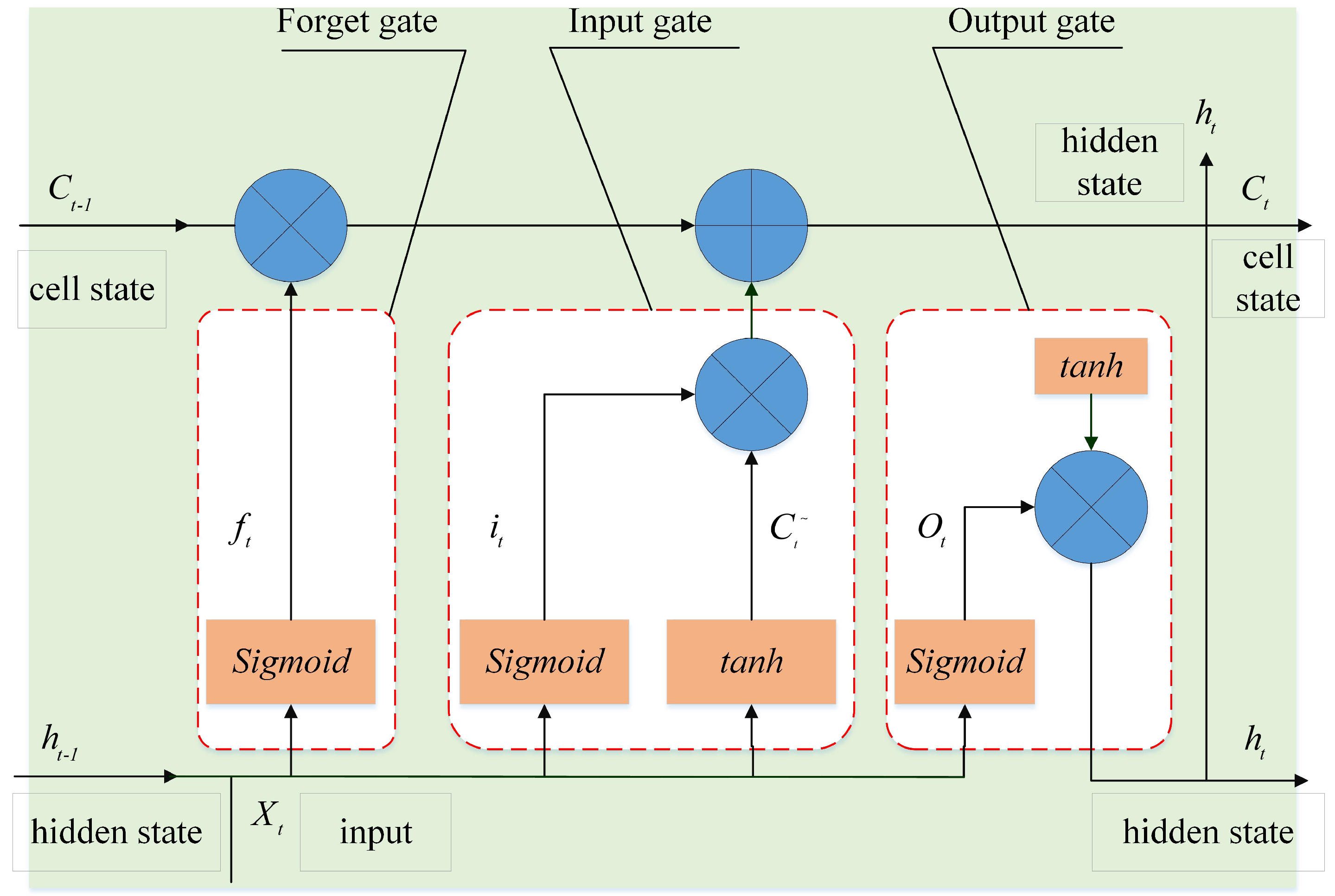
2.2. Long Short-Term Memory
2.3. Particle Swarm Optimization Algorithm
3. Methodology
3.1. A Framework for Predicting EC in Machining Systems
- (1)
- Data acquisition and storage
- (2)
- Data preprocessing
- (3)
- Data analysis
- (4)
- Application
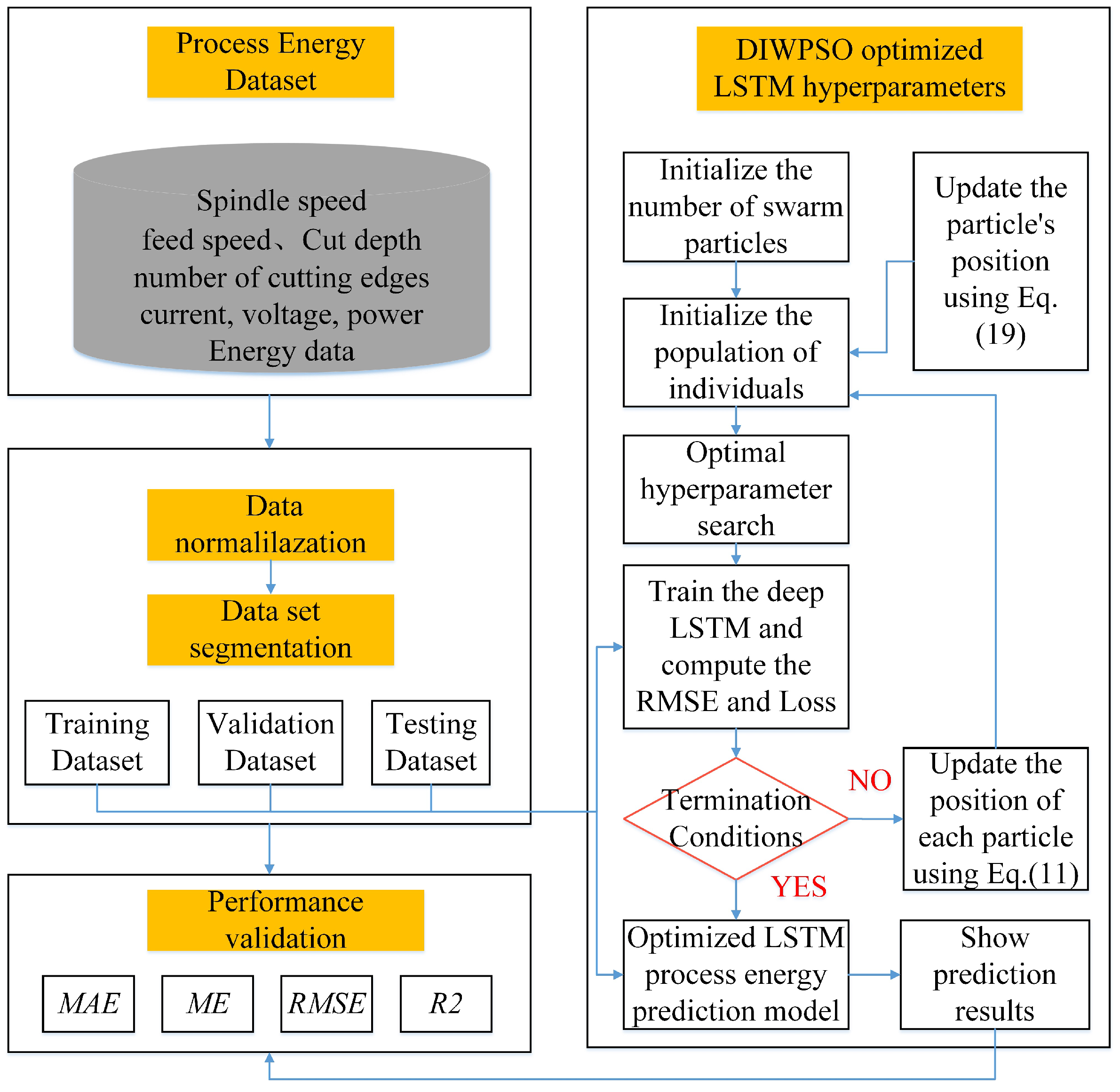
3.2. DIWPSO-LSTM: Energy Consumption Prediction Method
| Algorithm 1 Process energy prediction model based on DIWPSO-LSTM. |
|
4. Case Study
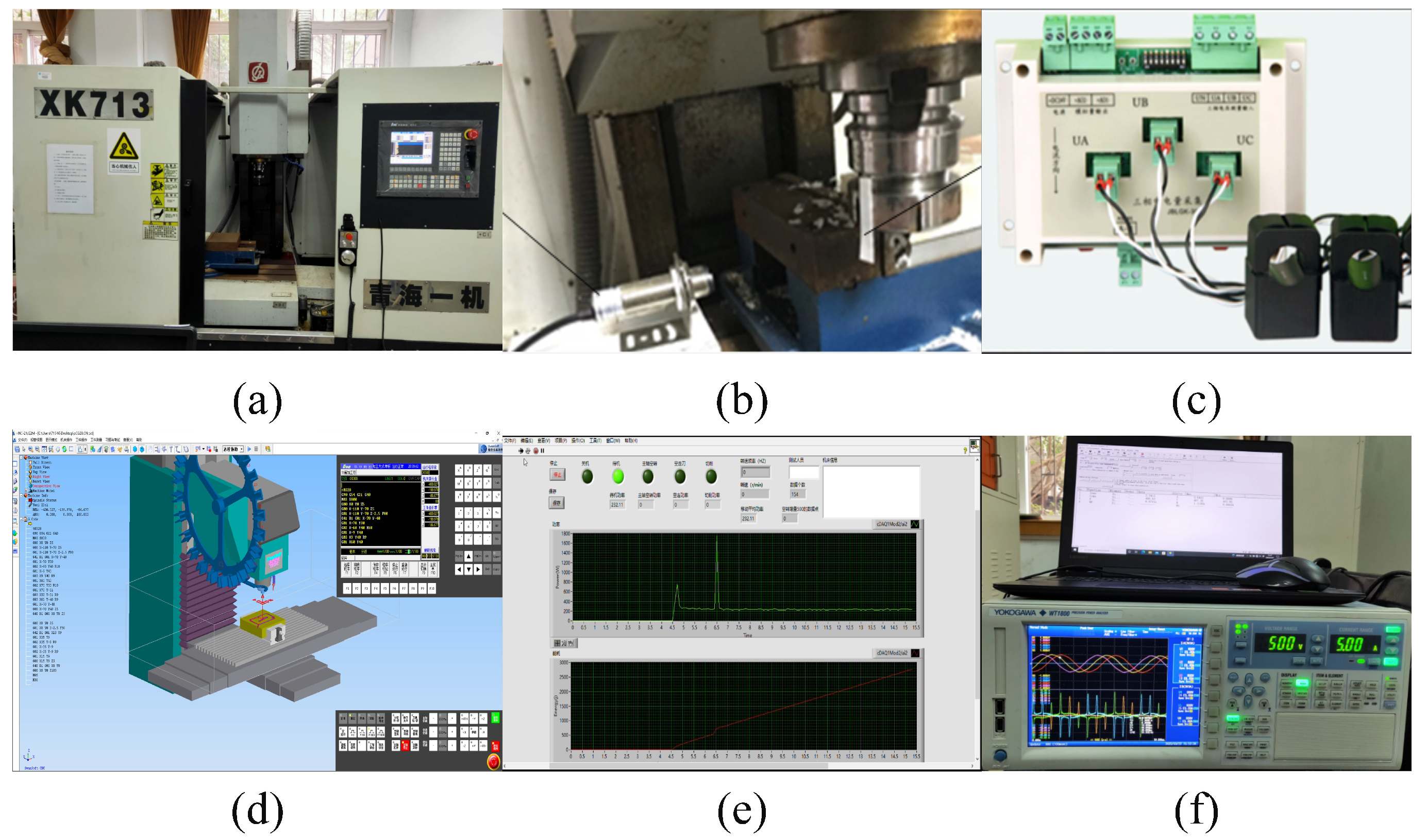
4.1. Construction of Experimental Platform
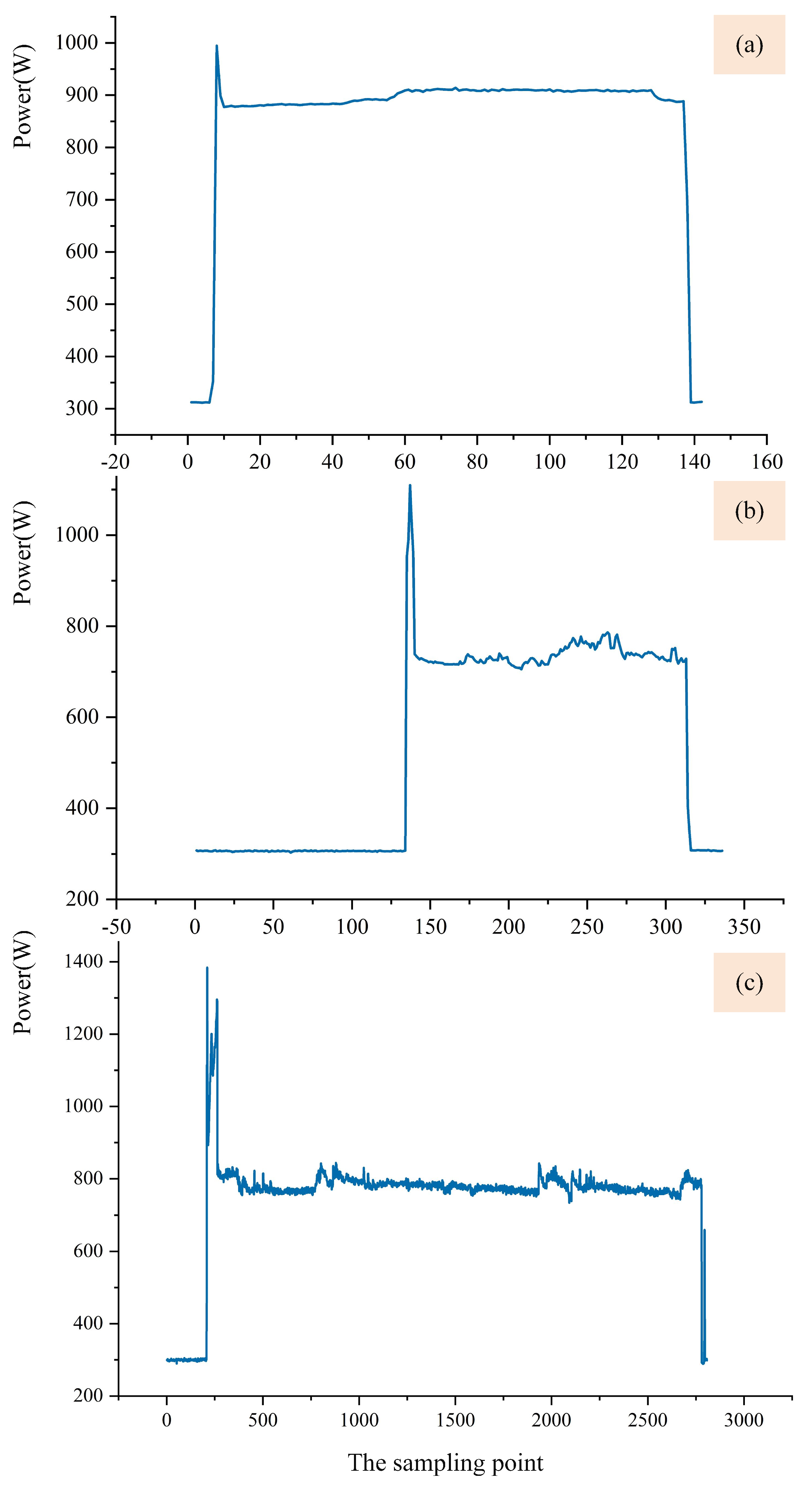
4.2. Process EC Dataset Construction
4.3. Model Parameter Settings
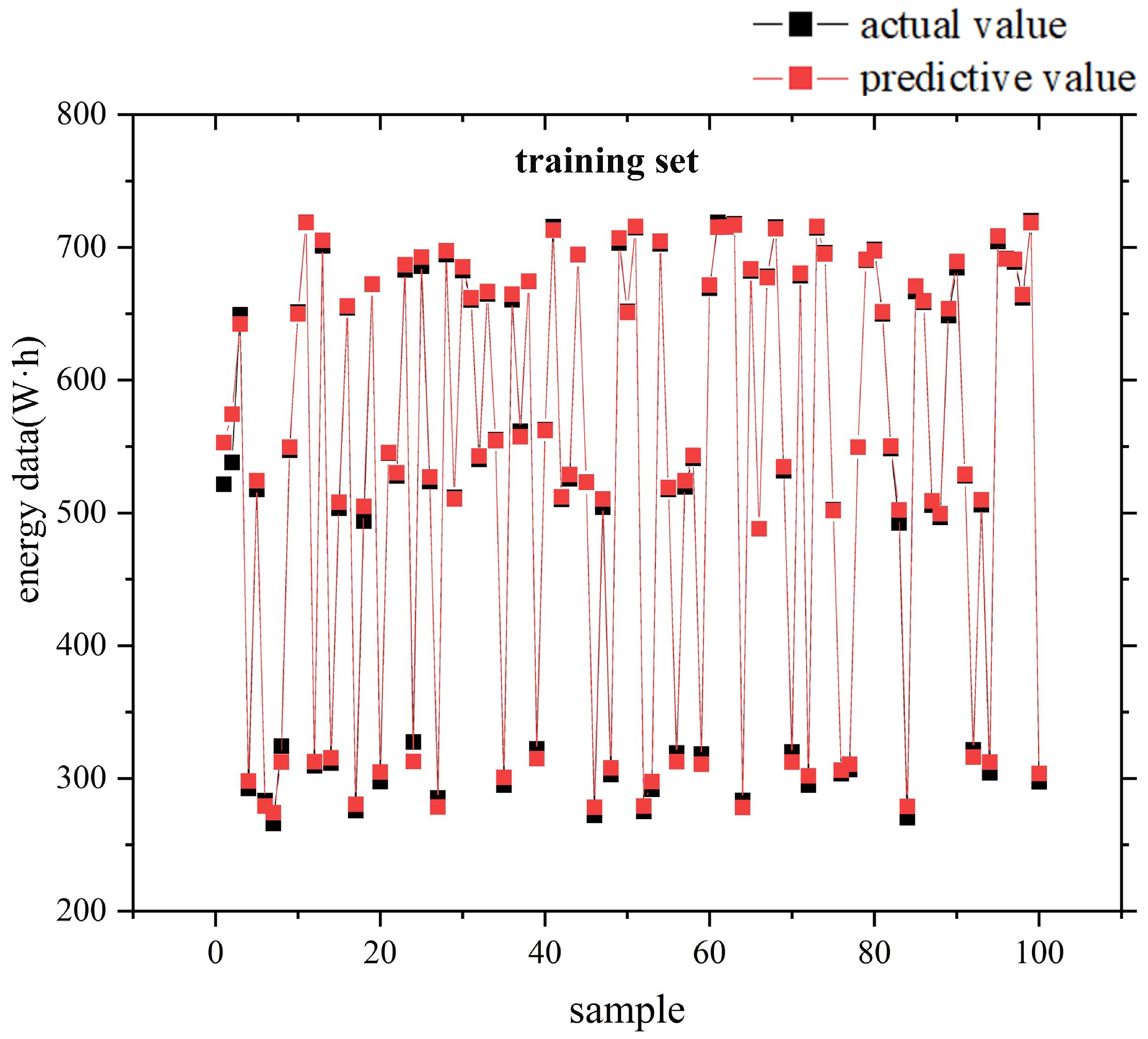
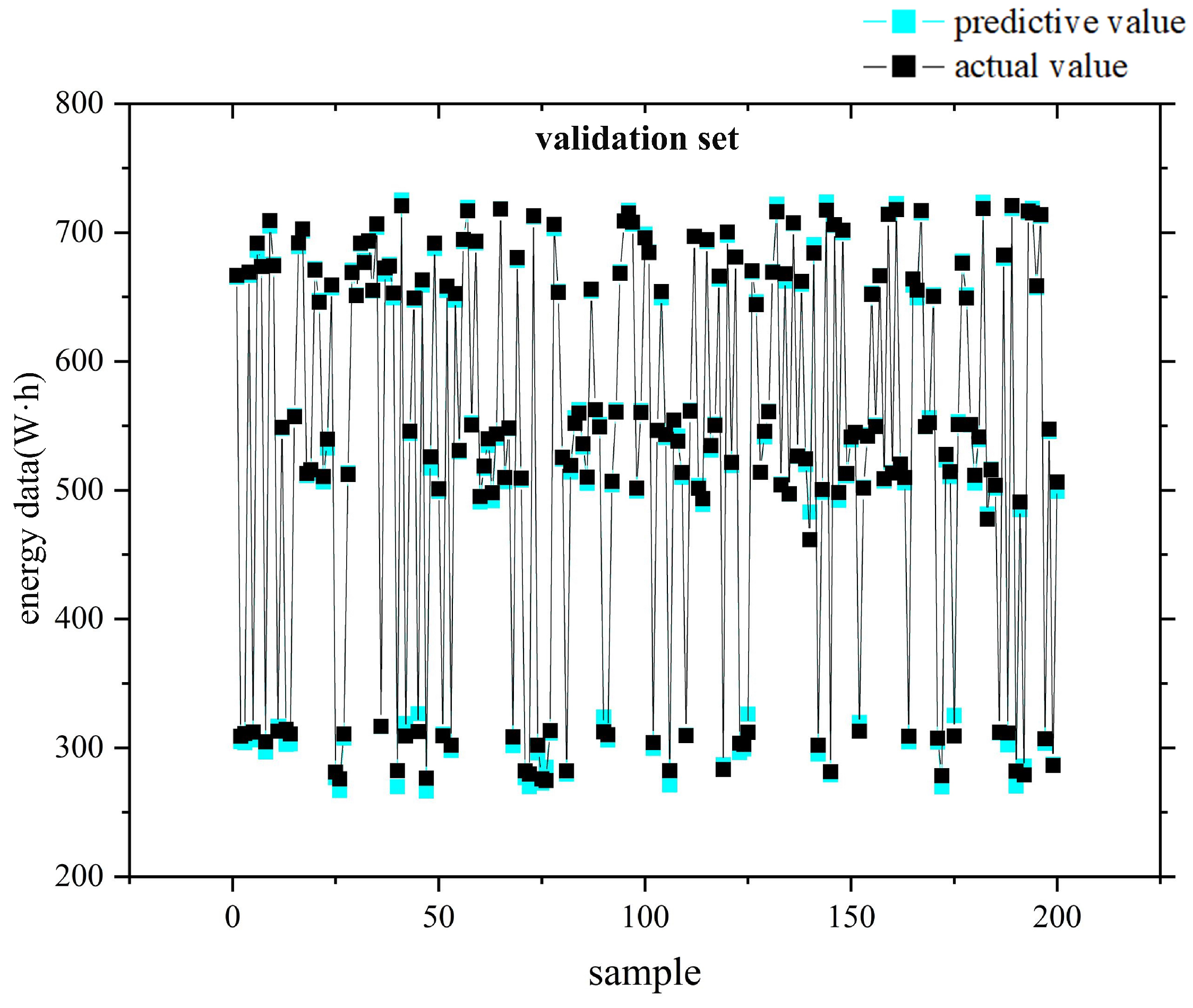
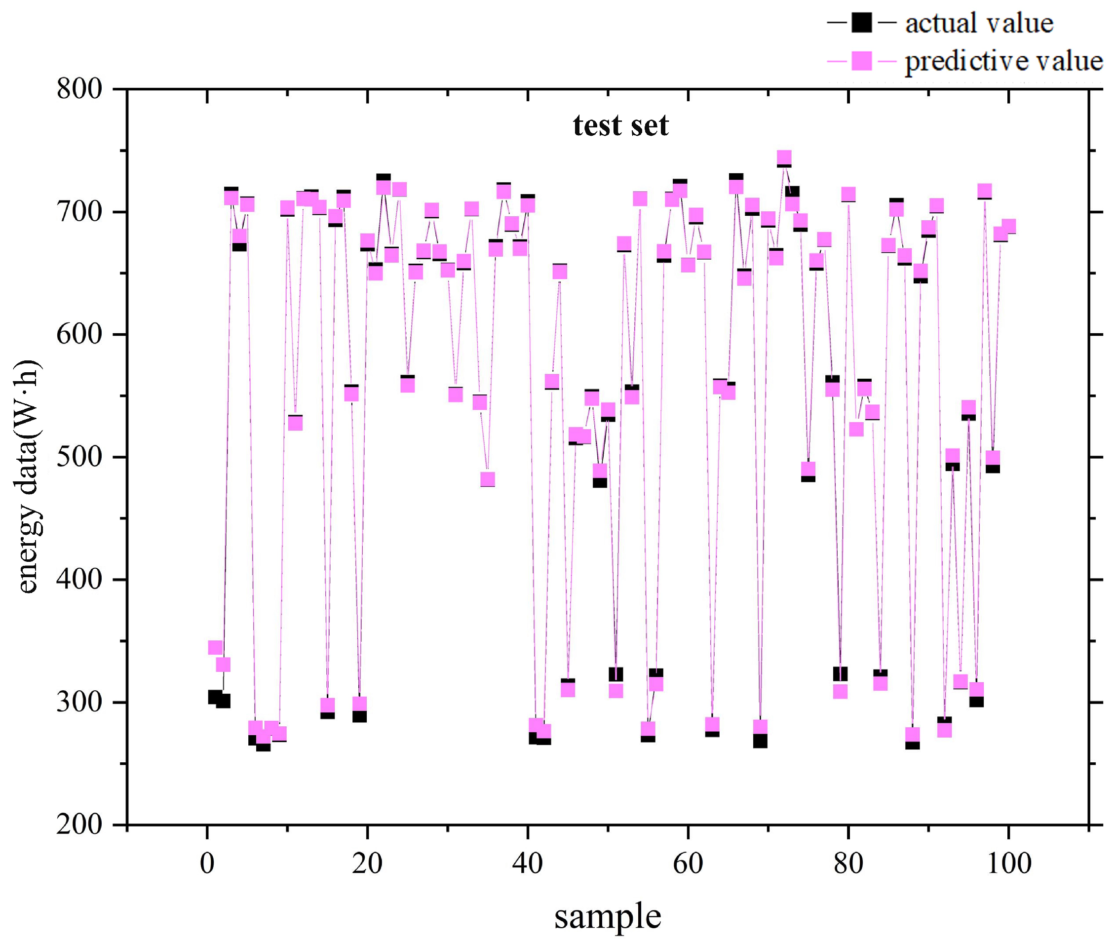
4.4. Results and Discussion
5. Conclusions
Author Contributions
Funding
Institutional Review Board Statement
Informed Consent Statement
Data Availability Statement
Conflicts of Interest
References
- Qi, R.; Shi, C.; Wang, M.Y. Carbon emission rush in response to the carbon reduction policy in China. China Inf. 2022, 37, 0920203X221093188. [Google Scholar] [CrossRef]
- Tracker, C.A. To Show Climate Leadership, US 2030 Target Should Be at Least 57%—63%. 2021. Available online: https://www.google.com.hk/url?sa=t&rct=j&q=&esrc=s&source=web&cd=&cad=rja&uact=8&ved=2ahUKEwjixt7ly_P9AhWTbN4KHXVaCioQFnoECA0QAw&url=https%3A%2F%2Fclimateactiontracker.org%2Fdocuments%2F846%2F2021_03_CAT_1.5C-consistent_US_NDC.pdf&usg=AOvVaw1I1hcAtVP-mj_lZUkqOp4P (accessed on 8 February 2023).
- Tsiropoulos, I.; Nijs, W.; Tarvydas, D.; Ruiz, P. Towards Net-Zero Emissions in the EU Energy System by 2050. Insights from Scenarios in Line with the 2020. Available online: https://publications.jrc.ec.europa.eu/repository/handle/JRC118592 (accessed on 8 February 2023).
- González-Torres, M.; Pérez-Lombard, L.; Coronel, J.F.; Maestre, I.R.; Yan, D. A review on buildings energy information: Trends, end-uses, fuels and drivers. Energy Rep. 2022, 8, 626–637. [Google Scholar] [CrossRef]
- Gadaleta, M.; Pellicciari, M.; Berselli, G. Optimization of the energy consumption of industrial robots for automatic code generation. Robot. Comput.-Integr. Manuf. 2019, 57, 452–464. [Google Scholar] [CrossRef]
- Giampieri, A.; Ling-Chin, J.; Ma, Z.; Smallbone, A.; Roskilly, A. A review of the current automotive manufacturing practice from an energy perspective. Appl. Energy 2020, 261, 114074. [Google Scholar] [CrossRef]
- Moradnazhad, M.; Unver, H.O. Energy efficiency of machining operations: A review. Proc. Inst. Mech. Eng. Part B J. Eng. Manuf. 2017, 231, 1871–1889. [Google Scholar] [CrossRef]
- Liu, N.; Zhang, Y.; Lu, W. A hybrid approach to energy consumption modelling based on cutting power: A milling case. J. Clean. Prod. 2015, 104, 264–272. [Google Scholar] [CrossRef]
- Shi, K.; Ren, J.; Wang, S.; Liu, N.; Liu, Z.; Zhang, D.; Lu, W. An improved cutting power-based model for evaluating total energy consumption in general end milling process. J. Clean. Prod. 2019, 231, 1330–1341. [Google Scholar] [CrossRef]
- Wang, L.; Meng, Y.; Ji, W.; Liu, X. Cutting energy consumption modelling for prismatic machining features. Int. J. Adv. Manuf. Technol. 2019, 103, 1657–1667. [Google Scholar] [CrossRef]
- He, Y.; Wang, L.; Wang, Y.; Li, Y.; Wang, S.; Wang, Y.; Liu, C.; Hao, C. An analytical model for predicting specific cutting energy in whirling milling process. J. Clean. Prod. 2019, 240, 118181. [Google Scholar] [CrossRef]
- Lv, J.; Tang, R.; Tang, W.; Liu, Y.; Zhang, Y.; Jia, S. An investigation into reducing the spindle acceleration energy consumption of machine tools. J. Clean. Prod. 2017, 143, 794–803. [Google Scholar] [CrossRef] [Green Version]
- Yuan, X.; Tan, Q.; Lei, X.; Yuan, Y.; Wu, X. Wind power prediction using hybrid autoregressive fractionally integrated moving average and least square support vector machine. Energy 2017, 129, 122–137. [Google Scholar] [CrossRef]
- Hu, L.; Peng, C.; Evans, S.; Peng, T.; Liu, Y.; Tang, R.; Tiwari, A. Minimising the machining energy consumption of a machine tool by sequencing the features of a part. Energy 2017, 121, 292–305. [Google Scholar] [CrossRef] [Green Version]
- Brillinger, M.; Wuwer, M.; Hadi, M.A.; Haas, F. Energy prediction for CNC machining with machine learning. CIRP J. Manuf. Sci. Technol. 2021, 35, 715–723. [Google Scholar] [CrossRef]
- LI, C.; Yin, Y.; Xiao, Q.; Long, Y.; Zhao, X. Data-driven Energy Consumption Prediction Method of CNC Turning Based on Meta-action. China Mech. Eng. 2020, 31, 2601. [Google Scholar]
- Qin, J.; Liu, Y.; Grosvenor, R. Multi-source data analytics for AM energy consumption prediction. Adv. Eng. Inform. 2018, 38, 840–850. [Google Scholar] [CrossRef]
- Liu, Z.; Guo, Y. A hybrid approach to integrate machine learning and process mechanics for the prediction of specific cutting energy. CIRP Ann. 2018, 67, 57–60. [Google Scholar] [CrossRef]
- Kim, Y.M.; Shin, S.J.; Cho, H.W. Predictive modeling for machining power based on multi-source transfer learning in metal cutting. Int. J. Precis. Eng. Manuf. Green Technol. 2022, 9, 107–125. [Google Scholar] [CrossRef]
- He, Y.; Wu, P.; Li, Y.; Wang, Y.; Tao, F.; Wang, Y. A generic energy prediction model of machine tools using deep learning algorithms. Appl. Energy 2020, 275, 115402. [Google Scholar] [CrossRef]
- Kahraman, A.; Kantardzic, M.; Kahraman, M.M.; Kotan, M. A data-driven multi-regime approach for predicting energy consumption. Energies 2021, 14, 6763. [Google Scholar] [CrossRef]
- Karijadi, I.; Chou, S.Y. A hybrid RF-LSTM based on CEEMDAN for improving the accuracy of building energy consumption prediction. Energy Build. 2022, 259, 111908. [Google Scholar] [CrossRef]
- Somu, N.; MR, G.R.; Ramamritham, K. A hybrid model for building energy consumption forecasting using long short term memory networks. Appl. Energy 2020, 261, 114131. [Google Scholar] [CrossRef]
- Luo, X.; Oyedele, L.O. Forecasting building energy consumption: Adaptive long-short term memory neural networks driven by genetic algorithm. Adv. Eng. Inform. 2021, 50, 101357. [Google Scholar] [CrossRef]
- Zhou, X.; Lin, W.; Kumar, R.; Cui, P.; Ma, Z. A data-driven strategy using long short term memory models and reinforcement learning to predict building electricity consumption. Appl. Energy 2022, 306, 118078. [Google Scholar] [CrossRef]
- Ullah, F.U.M.; Ullah, A.; Haq, I.U.; Rho, S.; Baik, S.W. Short-term prediction of residential power energy consumption via CNN and multi-layer bi-directional LSTM networks. IEEE Access 2019, 8, 123369–123380. [Google Scholar] [CrossRef]
- Salam, A.; El Hibaoui, A. Energy consumption prediction model with deep inception residual network inspiration and LSTM. Math. Comput. Simul. 2021, 190, 97–109. [Google Scholar] [CrossRef]
- Fan, S. Research on deep learning energy consumption prediction based on generating confrontation network. IEEE Access 2019, 7, 165143–165154. [Google Scholar] [CrossRef]
- Xiao, Q.; Li, C.; Tang, Y.; Chen, X. Energy efficiency modeling for configuration-dependent machining via machine learning: A comparative study. IEEE Trans. Autom. Sci. Eng. 2020, 18, 717–730. [Google Scholar] [CrossRef]
- Hochreiter, S.; Schmidhuber, J. Long short-term memory. Neural Comput. 1997, 9, 1735–1780. [Google Scholar] [CrossRef]
- Moreno, S.R.; da Silva, R.G.; Mariani, V.C.; dos Santos Coelho, L. Multi-step wind speed forecasting based on hybrid multi-stage decomposition model and long short-term memory neural network. Energy Convers. Manag. 2020, 213, 112869. [Google Scholar] [CrossRef]
- Wang, J.; Ma, Y.; Zhang, L.; Gao, R.X.; Wu, D. Deep learning for smart manufacturing: Methods and applications. J. Manuf. Syst. 2018, 48, 144–156. [Google Scholar] [CrossRef]
- Marini, F.; Walczak, B. Particle swarm optimization (PSO). A tutorial. Chemom. Intell. Lab. Syst. 2015, 149, 153–165. [Google Scholar] [CrossRef]
- Brand, M. Incremental singular value decomposition of uncertain data with missing values. In Proceedings of the European Conference on Computer Vision, Copenhagen, Denmark, 28–31 2002; Springer: Berlin/Heidelberg, Germany, 2002; pp. 707–720. [Google Scholar]
- Bai, Q. Analysis of particle swarm optimization algorithm. Comput. Inf. Sci. 2010, 3, 180. [Google Scholar] [CrossRef] [Green Version]


| Drilling Data | Milling Plane Data | Milling Slot Data | Data Ratio | |
|---|---|---|---|---|
| WT1800 PowerTester | 12,298 | 1936 | 10,587 | 70% |
| LabVIEW Programming | 1168 | 1072 | 1525 | 30% |
| Total data | 8959 | 1677 | 7868 | 100% |
| Time | Millisecond | Current (A) | Voltage (V) | Power (W) | Spindle Speed (r/min) | Feed Speed (r/min) | Depth of Cut | Number of Blades | Energy Consumption (W.h) |
|---|---|---|---|---|---|---|---|---|---|
| 15:48:40 | 289 | 0.587 | 406.22 | 298.4 | 1200 | 2000 | 2.5 | 4 | 261.307 |
| 15:48:40 | 388 | 0.585 | 406.22 | 298.2 | 1200 | 2000 | 2.5 | 4 | 261.317 |
| 15:48:41 | 199 | 0.585 | 405.85 | 297.7 | 1200 | 2000 | 2.5 | 4 | 261.399 |
| 15:48:51 | 181 | 3.539 | 405.28 | 1213.7 | 1200 | 2000 | 2.5 | 4 | 264.948 |
| 16:07:15 | 81 | 2.002 | 404.86 | 760.9 | 1800 | 2500 | 2.5 | 4 | 456.939 |
| 16:07:16 | 76 | 1.978 | 404.94 | 752.4 | 1800 | 2500 | 2.5 | 4 | 457.16 |
| 16:12:14 | 93 | 2.935 | 404.52 | 1043.9 | 2000 | 2000 | 2.5 | 4 | 514.282 |
| 16:12:27 | 779 | 2.728 | 404.37 | 1015.7 | 2000 | 2000 | 2.5 | 4 | 518.659 |
| 16:12:28 | 84 | 2.714 | 404.25 | 1013.4 | 2000 | 2000 | 2.5 | 4 | 518.723 |
| 16:12:41 | 61 | 2.737 | 404.64 | 1032.9 | 2000 | 2000 | 2.5 | 4 | 522.913 |
| 16:13:03 | 79 | 2.814 | 403.53 | 1014 | 1000 | 1500 | 2.5 | 4 | 529.826 |
| 16:13:13 | 877 | 2.675 | 403.92 | 786 | 1000 | 1500 | 2.5 | 4 | 533.22 |
| 16:31:27 | 490 | 2.163 | 405.02 | 790 | 1000 | 1500 | 2.5 | 4 | 705.344 |
| 16:32:53 | 155 | 1.969 | 404.51 | 761.3 | 1000 | 1500 | 2.5 | 4 | 726.112 |
| 16:32:53 | 471 | 1.964 | 404.55 | 753.2 | 1000 | 1500 | 2.5 | 4 | 726.16 |
| 15:52:11 | 605 | 2.605 | 405.21 | 954.2 | 1200 | 2000 | 2.5 | 4 | 327.364 |
| 15:52:15 | 289 | 2.514 | 405.5 | 955.7 | 1200 | 2000 | 2.5 | 4 | 328.471 |
| 16:28:09 | 74 | 2.138 | 405.03 | 298.4 | 1200 | 2000 | 2.5 | 4 | 655.898 |
| 16:30:59 | 970 | 2.083 | 404.64 | 771.6 | 1000 | 1500 | 2.5 | 4 | 698.641 |
| 16:41:01 | 670 | 1.934 | 405.75 | 755.7 | 800 | 1200 | 2.5 | 4 | 825.252 |
| 16:42:06 | 180 | 0.602 | 405.06 | 299.9 | 800 | 1200 | 2.5 | 4 | 840.396 |
| ... | ... | ... | ... | ... | ... | ... | ... | ... | ... |
| Hyperparameters | Initial Range Setting | Optimization Results |
|---|---|---|
| hiddenUnit_num (Hun) | [90, 200] | 146 |
| LearningRate (Lr) | [0.001, 0.15] | 0.01211 |
| LearnRateDropFactor (Lrdf) | [0.01, 0.5] | 0.2 |
| LearnRateDropPeriod (Lrdp) | [80, 200] | 125 |
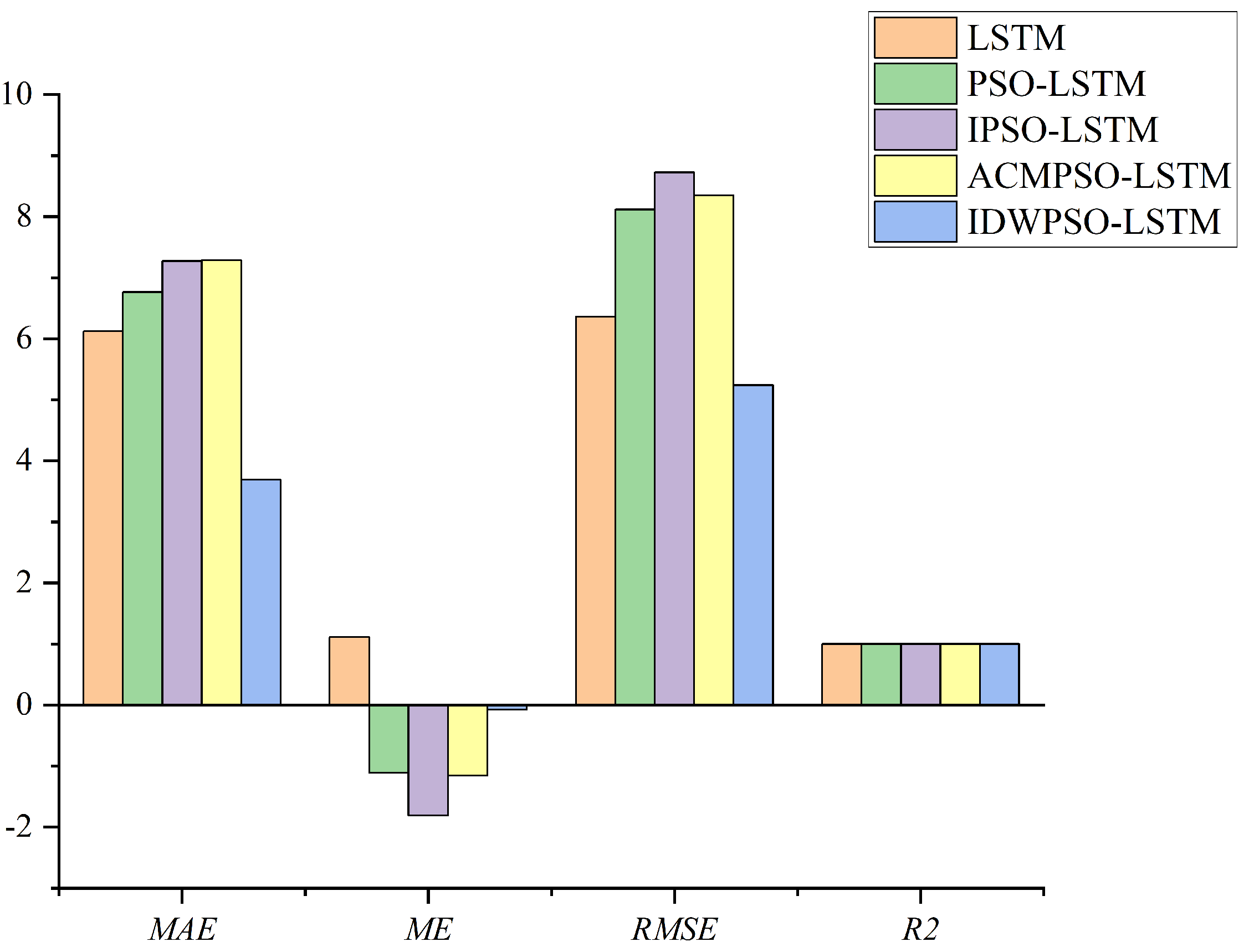
| MAE | ME | RMSE | R2 | |
|---|---|---|---|---|
| LSTM | 6.12214 | 1.11289 | 6.36465 | 0.99882 |
| PSO-LSTM | 6.76289 | −1.11015 | 8.11697 | 0.99885 |
| IPSO-LSTM | 7.27200 | −1.81000 | 8.72457 | 0.99830 |
| ACMPSO-LSTM | 7.28726 | −1.15409 | 8.35037 | 0.99863 |
| DIWPSO-LSTM | 3.68966 | −0.07248 | 5.23745 | 0.99891 |
| Optimization Time (Second) | Inertia Weight | Training Time (Second) | Network Layers Numbers | |
|---|---|---|---|---|
| PSO-LSTM | 371.0 | 0.80000 | 30.00000 | 4 |
| IPSO-LSTM | 374.0 | 0.80000 | 32.40000 | 4 |
| ACMPSO-LSTM | 391.3 | 0.77000 | 33.90000 | 4 |
| DIWPSO-LSTM | 331.1 | 0.97187 | 63.30000 | 7 |
Disclaimer/Publisher’s Note: The statements, opinions and data contained in all publications are solely those of the individual author(s) and contributor(s) and not of MDPI and/or the editor(s). MDPI and/or the editor(s) disclaim responsibility for any injury to people or property resulting from any ideas, methods, instructions or products referred to in the content. |
© 2023 by the authors. Licensee MDPI, Basel, Switzerland. This article is an open access article distributed under the terms and conditions of the Creative Commons Attribution (CC BY) license (https://creativecommons.org/licenses/by/4.0/).
Share and Cite
Zhang, M.; Zhang, H.; Yan, W.; Jiang, Z.; Zhu, S. An Integrated Deep-Learning-Based Approach for Energy Consumption Prediction of Machining Systems. Sustainability 2023, 15, 5781. https://doi.org/10.3390/su15075781
Zhang M, Zhang H, Yan W, Jiang Z, Zhu S. An Integrated Deep-Learning-Based Approach for Energy Consumption Prediction of Machining Systems. Sustainability. 2023; 15(7):5781. https://doi.org/10.3390/su15075781
Chicago/Turabian StyleZhang, Meihang, Hua Zhang, Wei Yan, Zhigang Jiang, and Shuo Zhu. 2023. "An Integrated Deep-Learning-Based Approach for Energy Consumption Prediction of Machining Systems" Sustainability 15, no. 7: 5781. https://doi.org/10.3390/su15075781