Optimal Control of Industrial Pollution under Stochastic Differential Models

Abstract

Considering that the amount of waste generated by an industrial enterprise is affected by many uncertain factors, such as the quality of raw materials and the state of equipment. The process is not deterministic, as assumed in most existing studies. In this paper, we propose a stochastic impulse control model to characterize the process of pollution control. The Quasi-Variational Inequality (QVI) method is implemented to solve the optimization problem. Our results show that the optimal control strategy for an industrial enterprise is to perform at a fixed intensity when the pollution reaches the threshold level. In addition, sensitivity analysis of parameters is implemented to illustrate the impact of higher growth rates and volatility on the optimal control strategy. The paper provides a decision basis for industrial enterprises to do pollution control efficiently.

1. Introduction

1.1. Research Questions

Problems of industrial pollution are common across the world, but there are subtle differences between developed and developing countries on this issue. Developed countries have transferred their most pollution-intensive manufacturing to developing countries through industrial transfer, and domestic pollution has been reduced. Developing countries, however, are under great pressure to balance economic growth with environmental protection. Copeland & Taylor (2001) [1] put forward that trade may tend to increase world pollution and provide added incentives for polluting industries to locate in countries with low environmental standards. Conversely, the income gains created by trade may increase the pressure for tougher environmental regulation and enforcement. This shows how difficult it is for developing countries to do industrial production under increasingly strict environmental regulations.

Most industrial enterprises are required to install wastewater and waste gas pollution control devices, but in operation, there are still some problems such as stealing discharge, substandard discharge, outages of devices, and a low rate of qualified devices. Why is that? The preliminary survey found that in practice, enterprises have concerns about the operation cost of pollution control devices and environmental costs, and frankly admitted that balancing economic benefits and environmental responsibility is a dilemma. To maximize profits, many companies turn on their pollution control devices only when the government comes to inspect them. The question of how to make the optimal decision considering the output, pollution amount, and pollution control cost has become an urgent problem for industrial enterprises. Considering that industrial pollution is mainly waste water, waste gas, and solid waste, this paper aims at the first two types of pollution which can be controlled through monitoring devices. Note that the amount of waste generated by an industrial enterprise is affected by many uncertain factors, such as the quality of raw materials and the state of pollution treatment devices [2,3,4]. The process is not deterministic, as assumed in most existing studies. In this paper, we propose a stochastic impulse control model [5,6] to characterize the process of wastewater discharge or waste gas emission. This study aims to answer the following research questions:

• How can industrial enterprises construct effective pollution control strategies and efficiently use pollution treatment devices to control the total amount of pollutants?
• How can industrial enterprises minimize the total expected discounted environmental costs (including environmental damage costs and pollution control costs) in pollution control?

The Quasi-Variational Inequality (QVI) method is implemented to solve the optimization problem. The rest of the paper is organized as follows. Section 2 briefly presents the industrial pollution control model, and Section 3 delivers QVI and the solution, and methodological details are relegated in Appendix A and Appendix B. The numerical study is obtained in Section 4. Conclusions and discussions of managerial implications are conducted in Section 5.

1.2. Novelty of the Current Study

The novelty of this work can be presented as follows:

• In addition to output, we take some stochastic factors into consideration when modeling the pollution treatment, which brings the model closer to reality.
• A new optimal control strategy is proposed to control the single industrial pollution of enterprises, which determines the starting time and intensity of pollution control in order to prevent the total amount of pollutants from being overloaded and to minimize the total cost of the enterprise.

1.3. Literature Review

Our work examines the optimal strategy for industrial enterprises to control pollution by means of a stochastic control model. This work is closely related to two research streams: industrial pollution and stochastic control.

Industrial pollution goes hand in hand with industrialization. It has long been the focus, debate, and discussion of academia (Robinson, 1985) [7]. Many early books proposed and systematically studied the concepts and methods of industrial pollution prevention and control (Freeman etc., 1992 [8]; Shen, 1995 [9]). Some studies investigated the components of pollutants in different types of industrial enterprises, such as pulp and paper industries and chemical industries, as well as how to deal with them technically (Sell, 1992 [10]; Arami etc., 2005 [11]; Zahrim etc., 2007 [12]). More recently, Orhon et al. (2009) [13] analyzed two selected industrial categories, textile and leather tanning industries, to discuss industrial pollution treatment by activated sludge. Rajeshwari et al. (2000) [14] reviewed the development of various reactors for the treatment of high-strength water pollution from selected industries to identify the critical factors affecting performance so that the reactor’s efficiency can be improved by maintaining optimal operating conditions. Muga and Mihelcic (2008) [15] investigated the sustainability of different pollution treatment technologies. Patwardhan (2017) [16] introduced flow measurement, characterization, and treatability studies of industrial pollution, as well as specific water pollution in many different industries, such as textile, dairy, slaughtering, tannery, sugar mill, and pulp and paper mill at al. Rosu et al. (2021) [17] Optimized the performance of a simulated pollution treatment plant by the relaxation method. Just as important as technology is the regulation of industrial pollution, especially in developing countries. Eskeland and Jimenez (1992) [18] analyzed policy instruments for pollution control in developing countries to seek cost-effective intervention.Afsah, Laplante, and Wheeler (1996) [19] call for a revised model for the regulation of industrial pollution. They think the traditional emphasis on appropriate policy instruments, while ultimately correct, is premature because agencies in most developing countries have too many problems with information and transaction costs to implement any instruments comprehensively. Pargal and Wheeler (1996) [20] studied informal regulation of industrial pollution in developing countries and found that when formal regulation is weak or absent, communities often use other channels to induce pollution abatement by local factories in a process of informal regulation. García, Sterner, and Afsah (2007) [21] studied the public disclosure of industrial pollution and the impact of industrial enterprise environmental behavior. Still, it is very difficult for local environmental protection agencies to supervise industrial enterprises’ behavior (Dong et al., 2016) [22]. It can be seen from the above that there is an abundance of research on pollution control technology and government regulation. These external forces have a great effect on the environmental behavior of industrial enterprises, but sometimes in vain. It is critical to figure out how to increase their self-awareness about environmental protection. Industrial enterprises should bear the primary responsibility for reducing toxicity from emissions and related environmental impacts (Corcoran et al., 2010) [23]. Sonune and Ghate (2004), Crini and Lichtfouse (2019), and Varjani et al. (2020) [24,25,26] studied all the advanced methods of pollution treatment and reuse and found that industrial enterprises utilize advanced technology and equipment. However, they are relatively expensive to operate, and both operating costs and effluent quality are sensitive to operational quality. Therefore, it is necessary to carry out pollution control research from the perspective of industrial enterprises to help them achieve both profits and a green reputation.

What is worth mentioning is the method we used. According to the previous analysis, industrial pollution control is not only related to output but also affected by some random factors. Therefore, this paper innovatively uses the stochastic impulse control model to characterize pollutants. Stochastic control theory has developed rapidly in recent years as an important part of control theory and stochastic optimization theory. Akella and Kumar (1986) [27], and Korn (1997) [28] define a single-machine, single-piece production system as a stochastic optimal control problem. On this basis, the structure of the optimal control strategy is obtained through analysis, and a threshold control strategy is given to minimize the discounted cost of inventory and backlog in an infinite period. Ohnishi and Tsujimura (2006) [29] examine an optimal impulse control problem of a stochastic system whose state follows a geometric Brownian motion. In order to solve this problem, it is expressed as a random impulse control problem and proved by Quasi-Variational Inequality (QVI). Cadenillas et al. (2006) [30] examined the issue of dividend optimization. They believed that the purpose of the firms was to maximize expected total discounted dividend payments. Due to the existence of a fixed transaction cost, the resulting mathematical problem becomes a mixed classical impulse stochastic control problem, and the analytic part of the problem’s solution is simplified to a second-order nonlinear differential equation of the QVI. Scholars investigated the stochastic inventory problem, which consisted of a mixture of diffusion and Poisson processes in the demand model, and the stochastic inventory problem consisting of a mixture of constant demand and Poisson processes. By using impulse control theory, the Bellman equation of dynamic programming problem is reduced to a set of QVI, and the optimal strategy is obtained (Cadenillas and Zapatero, 2000 [31]; Bensoussan and Sethi, 2009 [32]; Cadenillas et al., 2010 [33]). In a more recent paper, Bensoussan et al. (2012) [34] established an impulse control model and applied it to solve the problem of a central bank intervening in the foreign exchange market. Perera and Long (2017) [35], and Ouaret et al. (2018) [36] studied production and alternative strategies for deteriorating manufacturing systems that minimize the total expected discounted costs in the case of random demand and quality. Perera et al. (2020) [37] focused on the control strategy of an online service provider that tries to keep its demand for bandwidth below a certain threshold level to avoid server congestion.

2. The Model

First, we introduce the model notations in

Table 1. Summary of Model Notations.

Symbol	Description
$P\left(t\right)$	Pollution generated by the enterprise at time t when there is no pollution treatment
$\tilde{P}\left(t\right)$	Pollution generated by the enterprise at time t during the treatment period
$\gamma$	Intensity of pollution treatment
${\tau }_i$	The start time of the i-th pollution treatment period
$T_i$	The duration of the i-th pollution treatment period
s	Pollution treatment policy
$\mu$	The growth rate of the pollution when there is no treatment
$\sigma$	The volatility of the total pollution
$\tilde{\mu }$	The growth rate of pollution during the pollution treatment period
V	A positive threshold

:

We now briefly describe the model. Enterprises generate pollution as a byproduct of the production process. We assume that the pollution produced by the enterprise during the production process is uncertain. The enterprise attempts to keep its pollution below a certain threshold level to avoid environmental degradation and government punishment. The decision-maker, the enterprise, decides the timing and pollution treatment intensity. Our model supposes that the pollution generated by the enterprise follows a geometric Brownian motion. Let $P\left(t\right)$ denote pollution generated by the enterprise at time t when there is no treatment. Let $B\left(t\right)$ be a one-dimensional standard Brownian motion be defined on a probability space $\left(\Omega ,\mathcal{F},P\right)$ with an information filtration ${\left\{{\mathcal{F}}_t\right\}}_{t\ge 0}$. The total pollution $P\left(t\right)$ at time t when there is no treatment, which is the solution of the following stochastic differential equation (SDE):

$$\left\{\begin{array}{c}dP\left(t\right)=\mu P\left(t\right)dt+\sigma P\left(t\right)dB\left(t\right)\\ P\left(0\right)=x>0\end{array}\right.,$$

(1)

where $\mu >0$ is the net growth rate indicating the growth rate of pollutants minus the natural self-purification rate of pollution, and $\sigma$ is a positive parameter reflecting the volatility of the total pollution. We assume $P\left(0\right)=x>0$. We also suppose that x is sufficiently small so that we do not need pollution control when $t=0$.

Let $\tilde{P}\left(t\right)$ be the pollution generated by the enterprise at time t during the pollution treatment period. We consider $\gamma$, which indicates that the enterprise can abate its pollution by a pollution treatment intensity $\gamma$, where $0<\gamma \le 1$. If the amount of pollution generated by the enterprise is $P\left(t\right)$ when there is no pollution control, then the total pollutant that the enterprise has not abated is represented by $\tilde{P}\left(t\right)$. During the treatment period, the dynamics of the total pollutant is governed by the following SDE:

$$\left\{\begin{array}{c}d\tilde{P}\left(t\right)=\tilde{\mu }\tilde{P}\left(t\right)dt+\sigma \tilde{P}\left(t\right)dB\left(t\right)\\ \tilde{P}\left(0\right)=x>0\end{array}\right.,$$

(2)

where the growth rate $\tilde{\mu }≔\mu -\gamma \theta ,$is a decreasing function of pollution control intensity $\gamma$ during the pollution control period. Here, we assume that $\theta >0$ is the constant of proportionality. Then the growth rate $\tilde{\mu }$ during the pollution control period is negative with the assumption $\mu <\theta$ and $\gamma >\frac{\mu }{\theta }$. Thus, we know that from this expression up here $\tilde{\mu }<0<\mu$, which indicates that the growth rate of pollution during the period of treatment is lower than that of the period without treatment.

Definition 1. 

The control strategy of the enterprise is a double sequence$s:={\left\{\left({\tau }_i,{\gamma }_i\right)\right\}}_{i\ge 0}$, where${\tau }_i$is the start time of the i-th treatment period,${\gamma }_i$is intensity of treatment.

Let $P_x\left(t\right)$ denote the total pollutant stock process $P\left(t\right)$ with $P\left(0\right)=x$. We denote the start time of the i-th treatment period by ${\tau }_i$.$T_i$ is the duration of the i-th treatment period. We assume that $T_i’\mathrm{s}$ are independent and identically distributed, and has the distribution function $F_T$. Therefore, the corresponding pollution control process can be defined by

$$P_x^{\left(s\right)}\left(t\right)=\left\{\begin{array}{c}{P}_x\left(t\right);0\le t<{\tau }_1\\ {\tilde{P}}_{P_x^{\left(s\right)}\left({\tau }_i{}^{-}\right)}\left(t-{\tau }_i\right);{\tau }_i\le t\le {\tau }_i+T_i,i=1,2,\dots \\ P_{P_x^{\left(s\right)}\left({\tau }_i+T_i\right)}\left(t-{\tau }_i-T_i\right);{\tau }_i+T_i<t<{\tau }_{i+1},i=1,2,\dots \end{array}\right.$$

(3)

The whole process will produce some environmental costs, including the environmental damage cost and pollution treatment cost. The purpose of the enterprise is to determine the optimal pollution treatment strategy to minimize the total expected discounted future costs.

(1)

the environmental damage cost: $\beta P_x^{\left(s\right)}\left(t\right)$

(2)

The pollution treatment cost: $K+\frac{1}{2}c{\left(\gamma P_x^{\left(s\right)}\left(t\right)\right)}^2$

First, we denote the environmental damage cost by $f\left(·\right)$ with $f\left(P_x^{\left(s\right)}\left(t\right)\right):=\beta P_x^{\left(s\right)}\left(t\right)$, for $\beta >0$. We assume that the pollution damage can be quantified in monetary terms, as is common in the literature (Atasu et al., 2009 [38], Atasu and Subramanian, 2012 [39]). According to Chang et al. (2018) [40], the damage caused by the pollution can be well approximated by a linear function, measured by $\beta P_x^{\left(s\right)}\left(t\right)$, where $\beta >0$ is the damage parameter. The parameter $\beta$ reflects how important pollution to a given enterprise is relative to the revenue it generates.

Now let $K+\frac{1}{2}c{\left(\gamma P_x^{\left(s\right)}\left(t\right)\right)}^2$ donate the pollution treatment cost, where K and c are positive constants. We assume that enterprises pay a fixed cost on pollution treatment devices and equipment purchase or investment K in the first part, which does not depend on the intensity of pollution control. The second part is the proportional cost of treatment, which is proportional to the intensity of pollution treatment. The higher the intensity of treatment, the greater the enterprise’s emission reduction efforts and the higher the proportional cost of the enterprise. The total amount of pollution that the enterprise abates can be represented as $\gamma P_x^{\left(s\right)}\left(t\right)$. Then we suppose that the enterprise has a quadratic function of the abatement of total pollution $\frac{1}{2}c{\left(\gamma P_x^{\left(s\right)}\left(t\right)\right)}^2$, where c is the unit cost of pollution abatement.

The goal of the enterprise is to minimize total expected future discounted costs. For a given discount rate r > 0, an initial pollution level $x>0$ and a treatment policy s, we can define this cost objective as below.

$$C^{\left(s\right)}\left(x\right)=E\left[{{\displaystyle \int }}_0^{\infty }{e}^{-rt}f\left(P_x^{\left(s\right)}\left(t\right)\right)dt+{{\displaystyle \sum }}_{i=1}^{\infty }{e}^{-r{\tau }_i}\left\{K+\frac{1}{2}c{\left[{\gamma }_i{P}_x^{\left(s\right)}\left({\tau }_i{}^{-}\right)\right]}^2\right\}\right].$$

(4)

Let $\Phi$ denote the value function (optimal minimal cost) of our pollution control problem, i.e., for all x > 0,

$$\Phi x=inf\left\{C^{\left(s\right)}\left(x\right);s\in S\right\}=C^{\left(s^{*}\right)}\left(x\right),$$

(5)

where $s^{*}$ is the minimizer of $C^{\left(s\right)}\left(x\right)$ over S representing the optimal strategy that minimizes the total expected future discount cost.

Definition 2.  

S denotes a set of acceptable pollution control strategies, for all$x>0, s\in S$, satisfy the following conditions:

A unique solution$P_x^{\left(s\right)}\left(t\right),t\ge 0$,

(i) 

${}_{i\to \infty }{}^{lim}\tau {}_i=\infty ,a.s.$,

(ii) 

$E\left[{{\displaystyle \int }}_0^{\infty }{e}^{-rt}f\left(P_x^{\left(s\right)}\left(t\right)\right)dt\right]<\infty$,

(iii) 

$E\left[{\displaystyle \sum }_{i=1}^{\infty }{e}^{-r{\tau }_i}\left\{K+\frac{1}{2}c{\left[{\gamma }_i{P}_x^{\left(s\right)}\left({\tau }_i-\right)\right]}^2\right\}\right]<\infty$,

(iv) 

${\gamma }_i\in \left(0,1\right],for i=1,2,\dots ,and$

(v) 

${\gamma }_{i+1}-{\gamma }_i\ge T_i,for i=1,2,\dots$.

As we can see from conditions (i)–(vi) above, the enterprise’s pollution control strategy needs to meet the corresponding conditions. The first four conditions are relatively common in other literature (Bensoussan et al., 2012) [38], while the last two conditions are not common but necessary for a meaningful analysis in our model. For example, conditions (iii) and (iv) indicate that the environmental costs of the enterprise are limited. Condition (v) means that the enterprise needs to wait until the end of the current pollution treatment period before the next phase of treatment. We believe that this assumption is valid for our application. For example, if an enterprise’s total amount of pollution produced exceeds a certain threshold, pollution control is necessary. This restriction is also supported by the fact that the fixed costs and emission proportional costs for enterprises to control pollution are large enough to make frequent pollution controls uneconomical. We recognize that, under a more general acceptable strategy, it is theoretically possible to envisage the next pollution treatment period occurring simultaneously with this one. However, for the sake of our application and mathematical simplicity, we set that ${\gamma }_{i+1}-{\gamma }_i\ge T_i,for i=1,2,\dots$ finally.

3. Formulation of Mathematical Model

We use the dynamic programming method to solve the stochastic control problem of our paper. At first, the Quasi-Variational Inequality (QVI) related to the optimization problem in this paper is derived, and it is proved that the QVI control introduced below is the optimal impulse control for pollution treatment. Next, it is proved that there is a unique solution to the simultaneous equations, and a verification theorem is used to prove that the solution of the QVI is consistent with the optimal (minimum) environmental cost of the original problem. Finally, the existence and uniqueness of the optimal pollution treatment strategy are verified by numerical results.

In our paper, at any given state $x$, the enterprise can choose to start pollution control immediately or stay put. If the enterprise chooses one of the schemes and then controls the pollution according to the optimal pollution treatment strategy, the cost of the scheme should not be lower than the cost of the optimal strategy. At any given pollutant stock state $x$, the enterprise can choose the following two alternative strategies.

The enterprise carries out pollution treatment immediately with the state $x$, and then carries out pollution treatment according to the optimal control strategy after the pollution reaches the critical level.

$$K+\frac{1}{2}c{\left(\gamma x\right)}^2+{{\displaystyle \int }}_0^{\infty }E\left[{{\displaystyle \int }}_0^T{e}^{-rh}f\left({\tilde{P}}_x\left(h\right)\right)dh+e^{-rT}\Phi {\tilde{P}}_x\left(T\right)\left|T=t\right.\right]d{F}_T\left(t\right).$$

Similarly to Ohnishi and Tsujimura (2006) [29], let $M$ denote the intervention operator on the space of functions $\Phi$. The enterprise chooses this alternative strategy optimally over $\gamma \in \left(0,1\right)$. Therefore, we denote this cost expression by $M\Phi \left(x\right)$. The cost under this alternative policy is higher than that under the optimal policy, i.e., $\Phi \left(x\right)\le M\Phi \left(x\right)$.

$$M\Phi \left(x\right):=inf\left\{K+\frac{1}{2}c{\left(\gamma x\right)}^2+{{\displaystyle \int }}_0^{\infty }E\left[{{\displaystyle \int }}_0^T{e}^{-rh}f\left({\tilde{P}}_x\left(h\right)\right)dh+e^{-rT}\Phi {\tilde{P}}_x\left(T\right)\left|T=t\right.\right]d{F}_T\left(t\right);\gamma \in \left(0,1\right]\right\}.$$

(6)

Another alternative policy is that the enterprise stays put for a short duration of length $\epsilon >0$. After the pollutant stock reaches the threshold level, treatment shall be carried out according to the optimal control policy.

$$\left[{{\displaystyle \int }}_0^{\epsilon }{e}^{-rt}f\left(P_x\left(t\right)\right)dt+e^{-r\epsilon }\Phi P_x\left(\epsilon \right)\right].$$

The cost under this alternative policy is higher than that under the optimal policy $\Phi \left(x\right)$, i.e., for any $\epsilon >0$, $\Phi \left(x\right)\le E\left[{{\displaystyle \int }}_0^{\epsilon }{e}^{-rt}f\left(P_x\left(t\right)\right)dt+e^{-r\epsilon }\Phi P_x\left(\epsilon \right)\right]$.

Dividing both sides of the above expression by $\epsilon$ and rearranging the terms, we obtain

$$\frac{E\left[e^{-r\epsilon }\Phi P_x\left(\epsilon \right)\right]-\Phi \left(x\right)}{\epsilon }+\frac{E\left[{{\displaystyle \int }}_0^{\epsilon }{e}^{-rt}f\left(P_x\left(t\right)\right)dt\right]}{\epsilon }\ge 0.$$

Then, letting $\epsilon \to 0$, we obtain$A\Phi \left(x\right)+f\left(x\right)\ge 0$,

$$\begin{gathered} A\Phi \left(x\right):=\underset{\epsilon \to 0}{\lim } \frac{E\left[e^{-r\epsilon }\Phi P_x\left(\epsilon \right)\right]-\Phi \left(x\right)}{\epsilon } \\ =\mu x\frac{\partial \Phi \left(x\right)}{\partial x}+\frac{1}{2}{\sigma }^2{x}^2\frac{{\partial }^2\Phi \left(x\right)}{\partial x^2}-r\Phi \left(x\right). \end{gathered}$$

Proposition 1.

For a given$x>0$, the value function$\Phi \left(x\right)$of our pollution control problem, which is assumed to be continuously differentiable, satisfies the following the QVI:

$$\begin{gathered} \Phi \left(x\right)\le M\Phi \left(x\right), \\ A\Phi \left(x\right)+f\left(x\right)\ge 0, \\ \left[A\Phi \left(x\right)+f\left(x\right)\right]\left[\Phi \left(x\right)-M\Phi \left(x\right)\right]=0. \end{gathered}$$

We observe that the solution of the QVI divides the interval $\left[\left.0,\infty \right)\right.$ into two disjoint regions ${\mathsf{\Sigma }}_1$ and ${\mathsf{\Sigma }}_2$.

• A continuation region: ${\Sigma }_1=\left\{x:\Phi \left(x\right)<M\Phi \left(x\right) and A\Phi \left(x\right)+f\left(x\right)=0\right\}$
• A pollution control region: ${\Sigma }_2=\left\{x:\Phi \left(x\right)=M\Phi \left(x\right) and A\Phi \left(x\right)+f\left(x\right)>0\right\}$

When the total pollution is inside the continuous region, the enterprise does not need to take any action. When the total pollution reaches the boundary of the continuous region, the enterprise should take immediate action to control it.

The solution of the QVI is consistent with the solution of pollution control in this paper which is governed by a positive threshold $V$ and the intensity of pollution control $\mathsf{\Gamma }$. The optimal pollution control strategy is that when the total pollution reaches the threshold level V, the enterprise combines pollution control intensity with treatment intensity. The continuation region and a pollution control region are (0,V) and $\left[V,\infty \right)$, respectively.

The solution to Equation (1) is as follows:

$$P_x\left(t\right)=x \exp \left\{\left(\mu -\frac{1}{2}{\sigma }^2\right)t+\sigma B\left(t\right)\right\}.$$

Next, using the exponential moments of the process, it follows that, for $q\in ℝ$,

$$E\left[P_x{\left(t\right)}^q\right]=x^q exp \left\{\left[\left(\mu -\frac{1}{2}{\sigma }^2\right)q+\frac{1}{2}{\sigma }^2{q}^2\right]t\right\}.$$

(7)

A similar identity holds for $\tilde{P}$ process, i.e.,

$$E\left[{\left({\tilde{P}}_x\left(t\right)\right)}^q\right]=x^q\exp \left\{\left[\left(\mu -\gamma \theta -\frac{1}{2}{\sigma }^2\right)q+\frac{1}{2}{\sigma }^2{q}^2\right]t\right\}.$$

(8)

First of all, we pay our attention to the continuation region $\left.\left(0,V\right.\right]$, where $A\Phi \left(x\right)+f\left(x\right)=0$. According to Boyce and Prima (1997) [37], we can gather that when $x\in \left.\left(0,V\right.\right]$, the solution of $A\Phi \left(x\right)+f\left(x\right)=0$ as follows:

$$\begin{gathered} \mu x\frac{\partial \Phi \left(x\right)}{\partial x}+\frac{1}{2}{\sigma }^2{x}^2\frac{{\partial }^2\Phi \left(x\right)}{\partial x^2}-r\Phi \left(x\right)+f\left(x\right)=0, \\ \Phi \left(x\right)=a{x}^{{\alpha }_1}+b{x}^{{\alpha }_2}+\left(\frac{\beta }{r-\mu }\right)x, \end{gathered}$$

where ${\alpha }_1=\frac{\frac{1}{2}{\sigma }^2-\mu +\sqrt{{\left(\mu -\frac{1}{2}{\sigma }^2\right)}^2+2{\sigma }^{2}r}}{{\sigma }^2}$, ${\alpha }_2=\frac{\frac{1}{2}{\sigma }^2-\mu -\sqrt{{\left(\mu -\frac{1}{2}{\sigma }^2\right)}^2+2{\sigma }^{2}r}}{{\sigma }^2}$, $a$ and $b$ are constants that need to be determined.

Now we compute the cost of the no pollution control policy from (4). The cost of the no pollution control policy is as follows:

$$\begin{gathered} C^{\left(0\right)}\left(x\right)=E\left[{{\displaystyle \int }}_0^{\infty }{e}^{-rt}f(P_x^{\left(s\right)}\left(t\right)dt\right] \\ ={{\displaystyle \int }}_0^{\infty }{e}^{-rt}\mathsf{\beta }\mathrm{E}\left[(P_x^{\left(s\right)}\left(t\right)\right]dt \\ ={{\displaystyle \int }}_0^{\infty }{e}^{-rt}\beta x{e}^{\mu t}dt \\ =\left(\frac{\beta }{r-\mu }\right)x. \end{gathered}$$

We can know from condition ($\mathrm{iii}$), $\left(r-\mu \right)>0$. $\Phi \left(x\right)$ above should be no greater than the cost when there is no pollution control $C^{\left(0\right)}\left(x\right)$ for any $x\in \left.\left(0,V\right.\right]$. Therefore, we can gather that

$$0\le a{x}^{{\alpha }_1}+b{x}^{{\alpha }_2}+\left(\frac{\beta }{r-\mu }\right)x\le \left(\frac{\beta }{r-\mu }\right)x$$

(9)

We note from the definition from Boyce and Prima (1997) [41] that ${\alpha }_1>0$ and ${\alpha }_2<0$. Now, letting x→0 in the inequality on the right-hand side of (9), we can deduce that $b\le 0$; however, taking the limit x→0 in the inequality on the left-hand side of (9), we conclude that $b=0$. Consequently, for $x\in \left.\left(0,V\right.\right]$. Therefore, for any $x\in \left.\left(0,V\right.\right]$,

$$\Phi \left(x\right)=a{x}^{{\alpha }_1}+\left(\frac{\beta }{r-\mu }\right)x,$$

(10)

Next, we turn our attention to the pollution control region $\left[\left.V,\infty \right)\right.$, where $\Phi \left(x\right)=M\Phi \left(x\right)$. We assume that $F_T\left(t\right)=1-e^{-\lambda t}$ to compute $M\Phi \left(x\right)$ explicitly and simply. T follows an exponential distribution with rate $\lambda >0$. The corresponding cost Φ(x) can be written as

$$\begin{gathered} \Phi \left(x\right)=M\Phi \left(x\right)=inf\left\{K+\frac{1}{2}c{\left(\gamma x\right)}^2+{{\displaystyle \int }}_0^{\infty }E\left[{{\displaystyle \int }}_0^T{e}^{-rh}f\left({\tilde{P}}_x\left(h\right)\right)dh+ \\ {e}^{-rT}\Phi {\tilde{P}}_x\left(T\right)\left|T=t\right.\right]d{F}_T\left(t\right);\gamma \in \left(0,1\right]\right\}. \end{gathered}$$

We define

$$R\left(x,\gamma \right)≔{{\displaystyle \int }}_0^{\infty }E\left[{{\displaystyle \int }}_0^T{e}^{-rh}f\left({\tilde{P}}_x\left(h\right)\right)dh+e^{-rT}\Phi {\tilde{P}}_x\left(T\right)\left|T=t\right.\right]d{F}_T\left(t\right).$$

Therefore, we can gather that

$$\begin{gathered} R\left(x,\gamma \right)=\frac{\beta x}{\left(r-\mu +\gamma \theta +\lambda \right)} \\ +\frac{a\lambda x^{{\alpha }_1}}{\left[r-\left(\mu -\gamma \theta \right){\alpha }_1-\frac{1}{2}{\mathsf{\sigma }}^2{\alpha }_1\left({\alpha }_1-1\right)+\lambda \right]} \\ +\frac{\beta \lambda x}{\left(r-\mu \right)\left(r-\mu +\gamma \theta +\lambda \right)}. \end{gathered}$$

See Appendix A. for the specific solution process.

Consequently, we have

$$\Phi \left(x\right)=\left\{\begin{array}{c}a{x}^{{\alpha }_1}+\left(\frac{\beta }{r-\mu }\right)x,if x\in \left(0,V\right)\\ K+\frac{1}{2}c{\left(\Gamma x\right)}^2+R\left(V,\Gamma \right),if x\in \left[V,\infty \right)\end{array}\right.$$

(11)

Using the standard “principle of smooth fit” at the boundary V of the continuation region, we can derive the following two equations

$$a{V}^{{\alpha }_1}+\left(\frac{\beta }{r-\mu }\right)V=K+\frac{1}{2}c{\left(\Gamma V\right)}^2+R\left(V,\Gamma \right),$$

(12)

$$a{\alpha }_1{V}^{{\alpha }_1-1}+\left(\frac{\beta }{r-\mu }\right)=c{\mathsf{\Gamma }}^{2}V.$$

(13)

In addition, we set the function $G\left(\gamma \right):=K+\frac{1}{2}c{\left(\gamma V\right)}^2+R\left(V,\gamma \right)$. When $\gamma =\mathsf{\Gamma }$, $G\left(\gamma \right)$ should be minimized. Then we derive the first-order condition ${\left.G’\left(\gamma \right)\right|}_{\gamma =\mathsf{\Gamma }}=0$. We derive

$$c{V}^2\mathsf{\Gamma }+\frac{\partial }{\partial \mathsf{\Gamma }}R\left(V,\mathsf{\Gamma }\right)=0$$

(14)

Proposition 2. 

$\Phi \left(x\right)$is a solution to the QVI that is defined in Proposition 1. for$x\in \left(0,V\right)$. $\Phi \left(x\right)$was established to meet the following two conditions:

(i) 

$\Phi \left(x\right)<K+\underset{0<\gamma \le 1}{\inf }\left\{\frac{1}{2}c{\left(x\gamma \right)}^2+R\left(x,\gamma \right)\right\},$

(ii) 

$V>\frac{-\beta +\sqrt{{\beta }^2-4cr{\Gamma }^2\left(2\mu +{\sigma }^2-r\right)\left(K+R\left(V,\Gamma \right)\right)}}{2c{\Gamma }^2\left(2\mu +{\sigma }^2-r\right)}$.

The detailed proof process is shown in Appendix B.

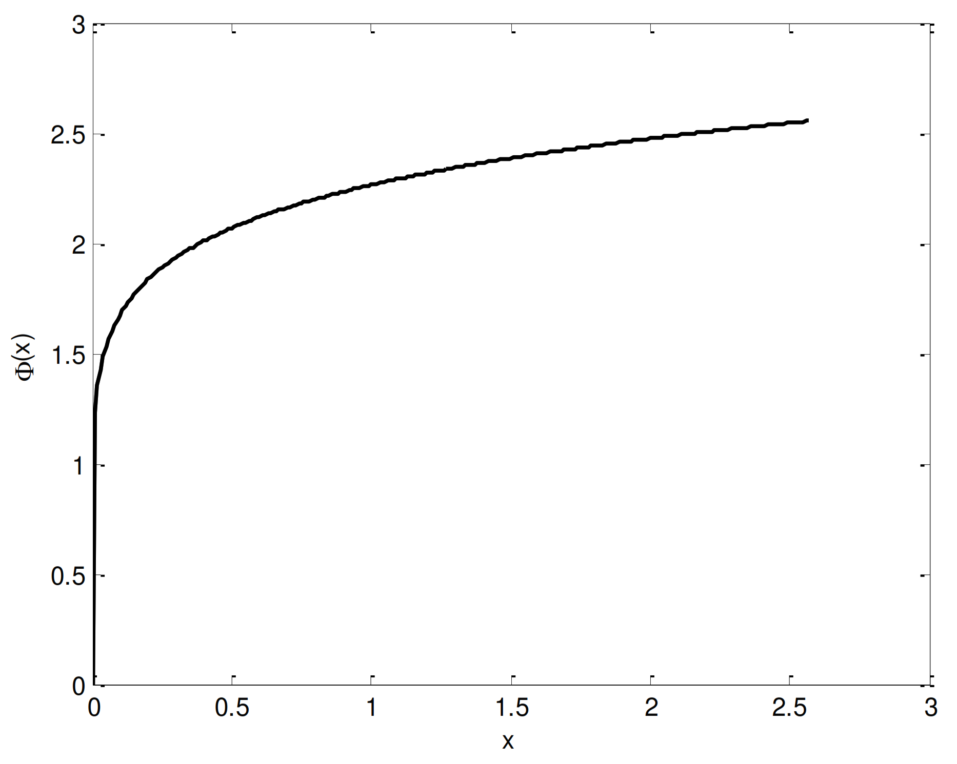
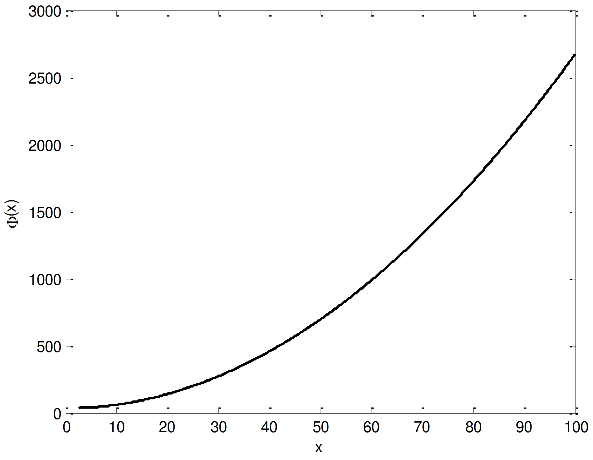
4. Numerical Computations and Sensitive Analysis

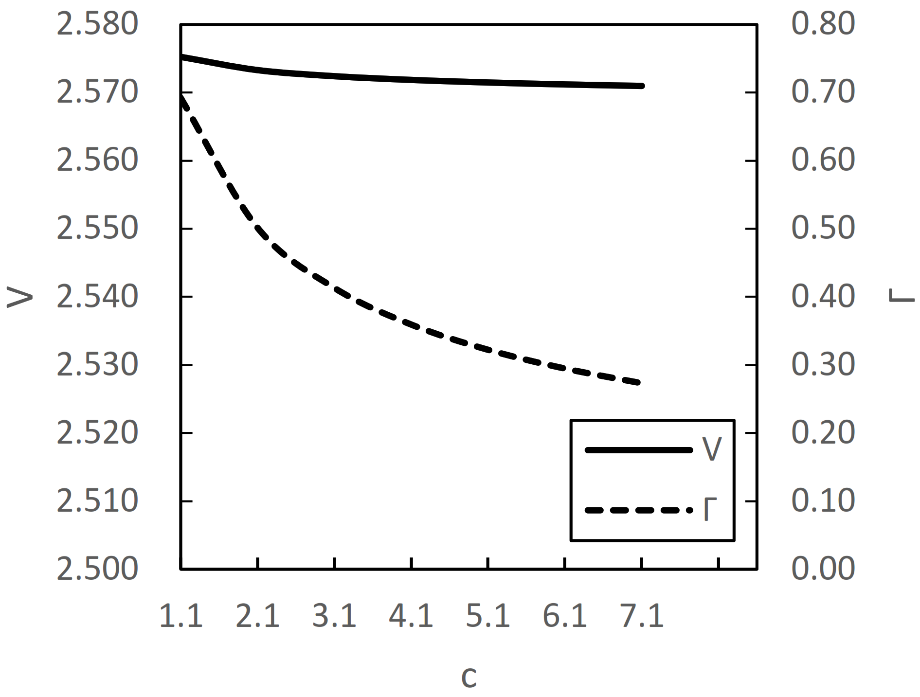
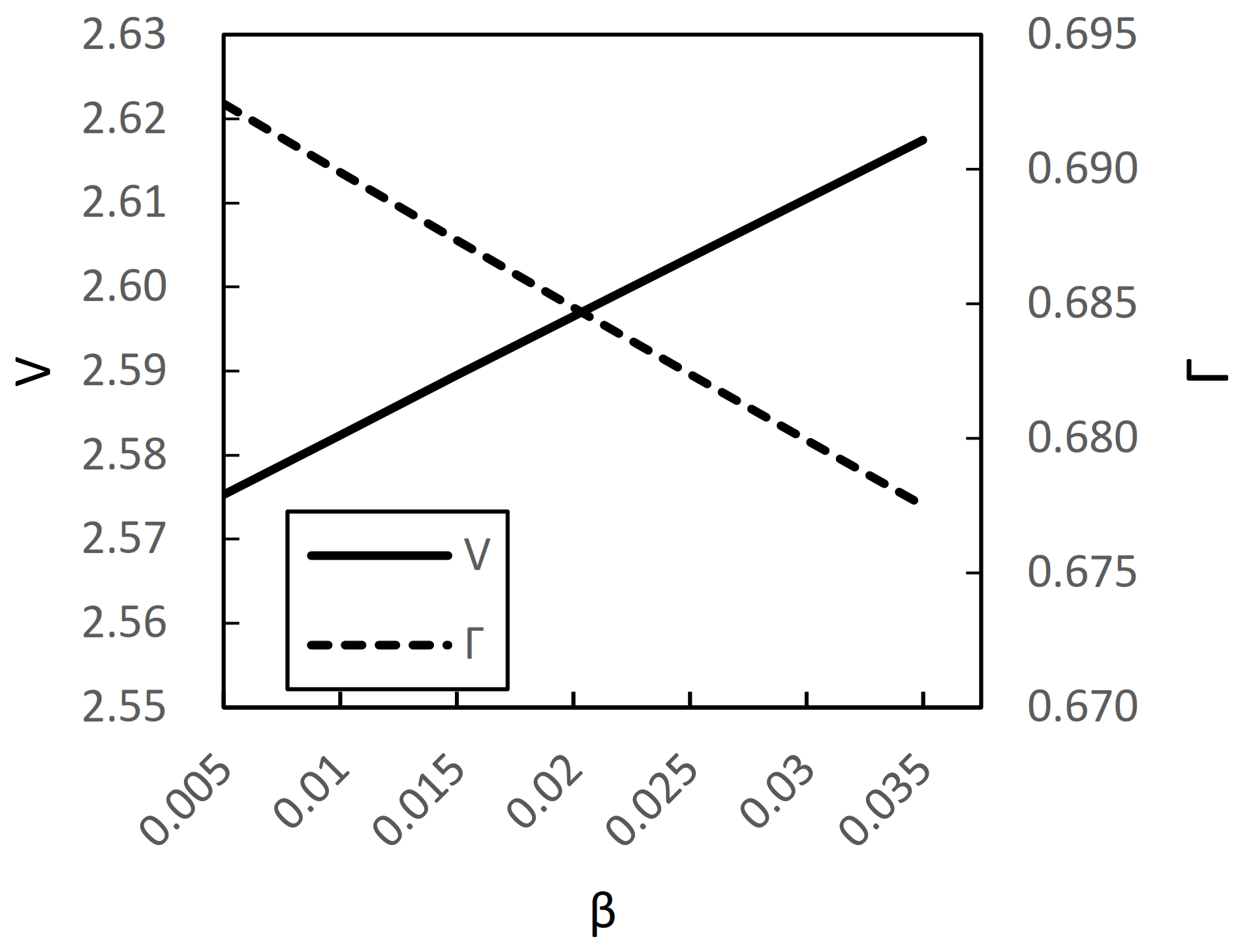
We use Newton’s method in MATLAB to solve the above nonlinear systems (12)–(14). Considering the admissibility constraints, convergence, existence, and uniqueness of the optimal solutions, we use the following parameters (see

Table 2. Baseline of parameters.

Parameters	μ	θ	σ	β	r	c	K	λ
Baseline	$0.70$	1.50	$0.50$	$0.005$	$0.08$	$1.1$	$20$	$0.1$

) in our baseline model:

Using our MATLAB program, we derive the numerical approximations (rounded to three decimal places) for V, and $\mathsf{\Gamma }$ as:

• V = 2.5753, $\mathsf{\Gamma }$ = 0.6925.

The inbuilt function in MATLAB provides the error range, and the conditions obtained for Equations (12)–(14) are verified to satisfy the default tolerance limit of the function of $1\times {10}^{-4}$ for the function. The above numerical solutions indicate that when the pollution amount of an enterprise reaches the level V = 2.5753, pollution control strategies should be adopted to reduce pollution emissions. In addition, intensity $\mathsf{\Gamma }$ = 0.6925 implies that the total amount of pollution should be reduced by 69.25% during the pollution control period. We used MATLAB to calculate the solutions of Equations (12)–(14), and then we carried out a comparative static analysis on the calculated solutions. Next, we use comparative static analysis to study the impact of each parameter in the model on the optimal pollution control strategy. Based on the above baseline values, we change the baseline value one at a time to observe the effect of its change on the pollution control threshold value and pollution treatment intensity in the pollution control strategy.

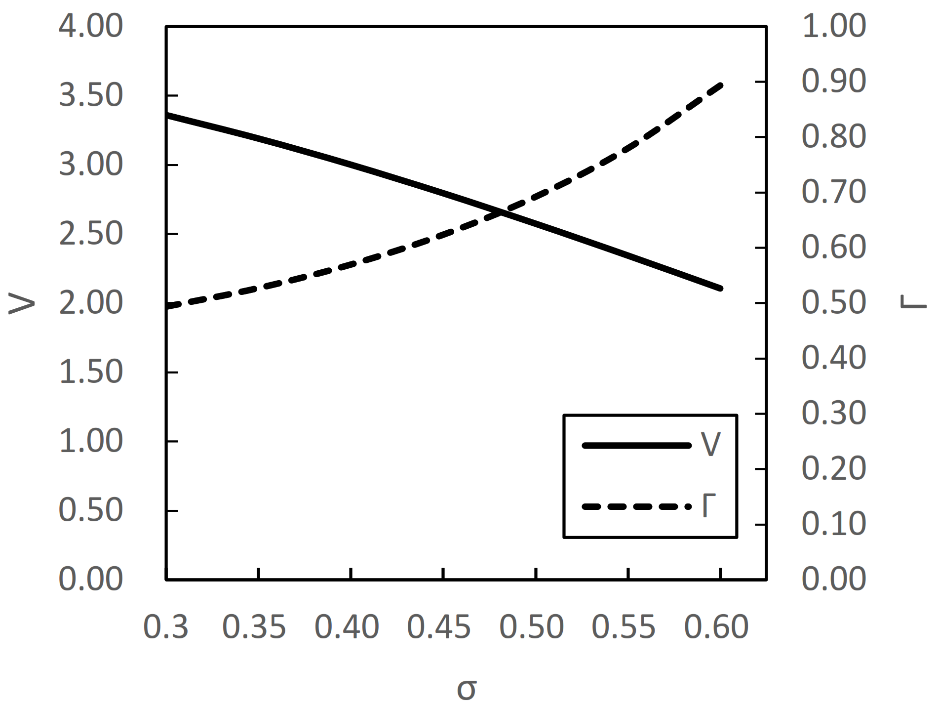
4.1. The Impact of Change on the Volatility

When $x\in \left(0,2.5753\right)$, the enterprise does not need to take measures to control the total pollution, it only needs to pay the environmental damage cost during this period. As can be seen from Figure 1, when the total pollution increases, the total environmental cost that enterprises need to pay will increase accordingly. Figure 2 shows that the enterprise should take immediate measures to control the total pollution for $x\in \left[2.5753,\infty \right)$, otherwise the total environmental cost of the enterprise will be increasing rapidly. This means that in order to reduce the total environmental cost of enterprises in the pollution control stage, enterprises should adopt the corresponding pollution control measures as soon as reaching the threshold.

As can be seen from Figure 3, the threshold of treatment V decreases with the increase of the volatility of total pollution σ, but the intensity of pollution control Γ increases with the increase of the volatility of total pollution σ. Therefore, we note from Figure 3 that when the fluctuation of pollution increases, the enterprise should take higher intensity pollution control measures to control pollution as early as possible.

Now let’s turn our attention to $\mathsf{\theta }$. We can see from Figure 4 that the greater $\mathsf{\theta }$ is, the greater the threshold value of pollution control will be, while the intensity of pollution control will increase. It should be noted that the growth rate of total pollution of enterprises during the pollution treatment period is $\mathsf{\mu }-\mathsf{\Gamma }\mathsf{\theta }$.

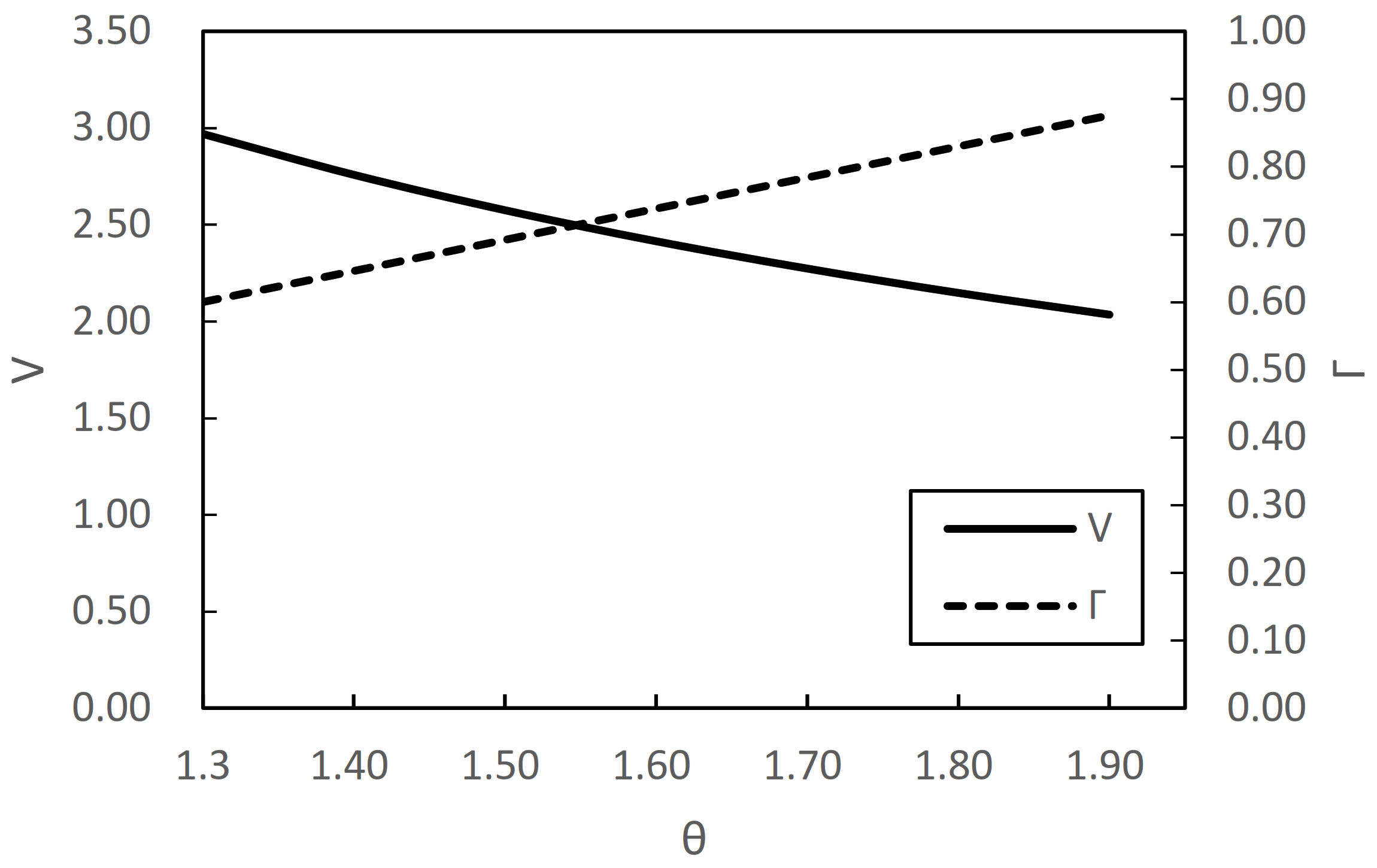
4.2. The Impact of Change in Cost Parameters

Figure 5 and Figure 6 show the impact of changes in the environmental cost parameters and the discount rate of the enterprise. Figure 5 illustrates that the unit cost of pollution abatement c representing the direct cost associated with pollution of the enterprise has an impact on the threshold and intensity of pollution control. Both Γ and V are decreasing at unit cost c. However, c has a greater impact on the pollution control intensity of enterprises. Hence, for a larger value of c, the enterprise should control pollution with less intensity and be patient before controlling it again. The value of c is directly related to the intensity of the pollution treatment by the enterprise and represents the proportional cost of pollution abatement.

We note from Figure 6 that for a larger value of the environmental damage parameter β, we expect a higher threshold of pollution control V and a smaller intensity Γ. As we explained in our model, the cost of environmental damage is the potential cost that enterprises pay for abating pollution. Thus, the higher the damage parameter β, the higher the environmental cost. This is why enterprises apply more intensive pollution controls at larger β values, thereby reducing the potential cost of their own.

5. Conclusions

In this study, we examined an optimal pollution control strategy for industrial enterprises that can minimize the environmental damage cost and pollution treatment cost paid by enterprises, at the same time control the pollution within the threshold value. In our optimal pollution control strategy, a positive threshold is proposed to deal with the pollution problem by introducing the intensity of the pollution treatment and the start time of the treatment period. We discussed the impact of two alternative strategies on the expected discounted future total costs. Moreover, we summarize the QVI associated with the value function of our problem. We prove that the solution of the QVI associated with our problem is a policy governed by a positive threshold V and a control factor $\mathsf{\Gamma }$. We draw the following conclusion: the enterprise has an optimal strategy as shown in Formula (11). This is to immediately turn on the pollution control facilities and adopt the pollution control intensity $\mathsf{\Gamma }$ to control the total pollution when the total pollution is detected to reach the threshold pollution level V. Under this strategy, the enterprise can achieve optimal pollution control with the minimum cost and achieve a balance between economic benefits and environmental benefits. The specific research conclusions are as follows: (1) The optimal pollution control strategy of an enterprise is directly related to the threshold value and total pollution control intensity. (2) The optimal control strategy is affected by the growth rate, volatility of total pollution, cost parameters, and discount rate of total pollution. (3) The optimization of environmental costs is related to the total amount of pollution. When the total amount of pollution is lower than the threshold value, the environmental cost increases to a certain extent with the total amount of pollution, but the impact is tolerable. When the total amount of pollution reaches or exceeds the threshold value, the total amount of the pollution’s impact on the environmental cost is more severe.

Some managerial insight can be obtained from the conclusion of this article. For developing countries where pollution-intensive industrial enterprises are concentrated, it is important to optimize the use of pollution treatment equipment and balance environmental protection and production. It is not reasonable for industrial enterprises to stealthily discharge pollution or leave the pollution treatment equipment idle. The total amount of pollution should be controlled, the threshold value V should be obtained, and the pollution control intensity should be determined to achieve the most economical pollution control. How do enterprises determine the threshold of total pollution? Mainly according to the emission permits they have. How do enterprises determine the intensity of pollution control? By means of pollution treatment devices. In short, this paper provides a new way of thinking for industrial enterprises in developing countries to carry out production activities efficiently on the basis of environmental regulations.

This study retains several limitations that call for further research. This article combines stochastic differential equations to characterize the randomness of pollution control, but if we can consider pollution abatement and the production–inventory control of enterprises, it will produce more interesting results.

References

1. Copeland, B.R.; Taylor, M.S. Trade and Transboundary Pollution 1. In The Economics of International Trade and the Environment; CRC Press: Boca Raton, FL, USA, 2001; pp. 119–142. [Google Scholar]
2. Bertinelli, L.; Camacho, C.; Zou, B. Carbon capture and storage and transboundary pollution: A differential game approach. Eur. J. Oper. Res. 2014, 237, 721–728. [Google Scholar] [CrossRef]
3. Sedakov, A.; Qiao, H.; Wang, S. A model of river pollution as a dynamic game with network externalities. Eur. J. Oper. Res. 2021, 290, 1136–1153. [Google Scholar] [CrossRef]
4. Yu, Q.-W.; Wu, F.-P.; Zhang, Z.-F.; Wan, Z.-C.; Shen, J.-Y.; Zhang, L.-N. Technical inefficiency, abatement cost and substitutability of industrial water pollutants in Jiangsu Province, China. J. Clean. Prod. 2021, 280, 124260. [Google Scholar] [CrossRef]
5. Ali, I.; Khan, S.U. Threshold of stochastic SIRS epidemic model from infectious to susceptible class with saturated incidence rate using spectral method. Symmetry 2022, 14, 1838. [Google Scholar] [CrossRef]
6. Ali, I.; Khan, S.U. Asymptotic Behavior of Three Connected Stochastic Delay Neoclassical Growth Systems Using Spectral Technique. Mathematics 2022, 10, 3639. [Google Scholar] [CrossRef]
7. Robison, H.D. Who pays for industrial pollution abatement? Rev. Econ. Stat. 1985, 67, 702–706. [Google Scholar] [CrossRef]
8. Freeman, H.; Harten, T.; Springer, J.; Randall, P.; Curran, M.A.; Stone, K. Industrial pollution prevention! A critical review. J. Air Waste Manag. Assoc. 1992, 42, 618–656. [Google Scholar] [CrossRef]
9. Shen, T.T.; Shen, T.T. Industrial Pollution Prevention; Springer: Berlin/Heidelberg, Germany, 1995. [Google Scholar]
10. Sell, N.J. Industrial Pollution Control: Issues and Techniques; John Wiley & Sons: Hoboken, NJ, USA, 1992. [Google Scholar]
11. Arami, M.; Limaee, N.Y.; Mahmoodi, N.M.; Tabrizi, N.S. Removal of dyes from colored textile wastewater by orange peel adsorbent: Equilibrium and kinetic studies. J. Colloid Interface Sci. 2005, 288, 371–376. [Google Scholar] [CrossRef]
12. Zahrim, A.Y.; Gilbert, M.L.; Janaun, J. Treatment of Pulp and Paper Mill Effluent Using Photo-fentons Process. J. Appl. Sci. 2007, 7, 2164–2167. [Google Scholar] [CrossRef] [Green Version]
13. Orhon, D.; Babuna, F.G.; Karahan, O. Industrial Wastewater Treatment by Activated Sludge; IWA Publishing: London, UK, 2009. [Google Scholar]
14. Rajeshwari, K.; Balakrishnan, M.; Kansal, A.; Lata, K.; Kishore, V. State-of-the-art of anaerobic digestion technology for industrial wastewater treatment. Renew. Sustain. Energy Rev. 2000, 4, 135–156. [Google Scholar] [CrossRef]
15. Muga, H.E.; Mihelcic, J.R. Sustainability of wastewater treatment technologies. J. Environ. Manag. 2008, 88, 437–447. [Google Scholar] [CrossRef]
16. Patwardhan, A.D. Industrial Wastewater Treatment; PHI Learning Pvt. Ltd.: New Delhi, India, 2017. [Google Scholar]
17. Rosu, B.; Condrachi, L.; Rosu, A.; Arseni, M.; Murariu, G. Optimizing the Performance of a Simulated Wastewater Treatment Plant by the Relaxation Method. EIRP Proc. 2021, 16. [Google Scholar]
18. Eskeland, G.S.; Jimenez, E. Policy instruments for pollution control in developing countries. World Bank Res. Obs. 1992, 7, 145–169. [Google Scholar] [CrossRef] [Green Version]
19. Afsah, S.; Laplante, B.; Wheeler, D. Controlling Industrial Pollution: A New Paradigm; SSRN: Rochester, NY, USA, 1996. [Google Scholar]
20. Pargal, S.; Wheeler, D. Informal regulation of industrial pollution in developing countries: Evidence from Indonesia. J. Political Econ. 1996, 104, 1314–1327. [Google Scholar] [CrossRef]
21. García, J.H.; Sterner, T.; Afsah, S. Public disclosure of industrial pollution: The PROPER approach for Indonesia? Environ. Dev. Econ. 2007, 12, 739–756. [Google Scholar] [CrossRef] [Green Version]
22. Dong, L.; Fujita, T.; Dai, M.; Geng, Y.; Ren, J.; Fujii, M.; Wang, Y.; Ohnishi, S. Towards preventative eco-industrial development: An industrial and urban symbiosis case in one typical industrial city in China. J. Clean. Prod. 2016, 114, 387–400. [Google Scholar] [CrossRef]
23. Corcoran, E.; Nellemann, C.; Baker, E.; Bos, R.; Osborn, D.; Savelli, H. The central role of wastewater management in sustainable development. A Rapid Response Assessment. United Nations Environment Programme, UN-HABITAT, GRID-Arendal. J. Environ. Prot. 2010, 3, 12–29. [Google Scholar]
24. Sonune, A.; Ghate, R. Developments in wastewater treatment methods. Desalination 2004, 167, 55–63. [Google Scholar] [CrossRef]
25. Crini, G.; Lichtfouse, E. Advantages and disadvantages of techniques used for wastewater treatment. Environ. Chem. Lett. 2019, 17, 145–155. [Google Scholar] [CrossRef]
26. Varjani, S.; Joshi, R.; Srivastava, V.K.; Ngo, H.H.; Guo, W. Treatment of wastewater from petroleum industry: Current practices and perspectives. Environ. Sci. Pollut. Res. 2020, 27, 27172–27180. [Google Scholar] [CrossRef]
27. Akella, R.; Kumar, P. Optimal control of production rate in a failure prone manufacturing system. IEEE Trans. Autom. Control 1986, 31, 116–126. [Google Scholar] [CrossRef] [Green Version]
28. Korn, R. Optimal impulse control when control actions have random consequences. Math. Oper. Res. 1997, 22, 639–667. [Google Scholar] [CrossRef]
29. Ohnishi, M.; Tsujimura, M. An impulse control of a geometric Brownian motion with quadratic costs. Eur. J. Oper. Res. 2006, 168, 311–321. [Google Scholar] [CrossRef]
30. Cadenillas, A.; Choulli, T.; Taksar, M.; Zhang, L. Classical and impulse stochastic control for the optimization of the dividend and risk policies of an insurance firm. Math. Financ. Int. J. Math. Stat. Financ. Econ. 2006, 16, 181–202. [Google Scholar] [CrossRef]
31. Cadenillas, A.; Zapatero, F. Classical and impulse stochastic control of the exchange rate using interest rates and reserves. Math. Financ. 2000, 10, 141–156. [Google Scholar] [CrossRef]
32. Bensoussan, A.; Liu, R.H.; Sethi, S.P. Optimality of an (s,S) policy with compound Poisson and diffusion demands: A quasi-variational inequalities approach. SIAM J. Control Optim. 2005, 44, 1650–1676. [Google Scholar] [CrossRef]
33. Cadenillas, A.; Lakner, P.; Pinedo, M. Optimal control of a mean-reverting inventory. Oper. Res. 2010, 58, 1697–1710. [Google Scholar] [CrossRef] [Green Version]
34. Bensoussan, A.; Long, H.; Perera, S.; Sethi, S. Impulse control with random reaction periods: A central bank intervention problem. Oper. Res. Lett. 2012, 40, 425–430. [Google Scholar] [CrossRef]
35. Perera, S.; Long, H. An approximation scheme for impulse control with random reaction periods. Oper. Res. Lett. 2017, 45, 585–591. [Google Scholar] [CrossRef]
36. Ouaret, S.; Kenné, J.P.; Gharbi, A. Production and replacement policies for a deteriorating manufacturing system under random demand and quality. Eur. J. Oper. Res. 2018, 264, 623–636. [Google Scholar] [CrossRef]
37. Perera, S.; Gupta, V.; Buckley, W. Management of online server congestion using optimal demand throttling. Eur. J. Oper. Res. 2020, 285, 324–342. [Google Scholar] [CrossRef]
38. Atasu, A.; Van Wassenhove, L.N.; Sarvary, M. Efficient take-back legislation. Prod. Oper. Manag. 2009, 18, 243–258. [Google Scholar] [CrossRef]
39. Atasu, A.; Subramanian, R. Extended producer responsibility for e-waste: Individual or collective producer responsibility? Prod. Oper. Manag. 2012, 21, 1042–1059. [Google Scholar] [CrossRef]
40. Chang, S.; Qin, W.; Wang, X. Dynamic optimal strategies in transboundary pollution game under learning by doing. Phys. A Stat. Mech. Its Appl. 2018, 490, 139–147. [Google Scholar] [CrossRef]
41. Kohler, W.E.; Johnson, L.W. Elementary Differential Equations; Pearson Addison-Wesley: Boston, MA, USA, 2006. [Google Scholar]
Figure 1. The impact of change in x for x ∈ (0, 2.5753).
Sustainability 15 05609 g001
Figure 2. The impact of change in x for x 2.5753 , .
Sustainability 15 05609 g002
Figure 3. Optimal pollution treatment intensity and threshold as σ increase.
Sustainability 15 05609 g003
Figure 4. Optimal pollution treatment intensity and threshold as θ increase.
Sustainability 15 05609 g004
Figure 5. Optimal pollution treatment intensity and threshold as c increase.
Sustainability 15 05609 g005
Figure 6. Optimal pollution treatment intensity and threshold as β increase.
Sustainability 15 05609 g006