
Characteristic Evaluation of Wind Power Distributed Generation Sizing in Distribution System
Abstract
:1. Introduction
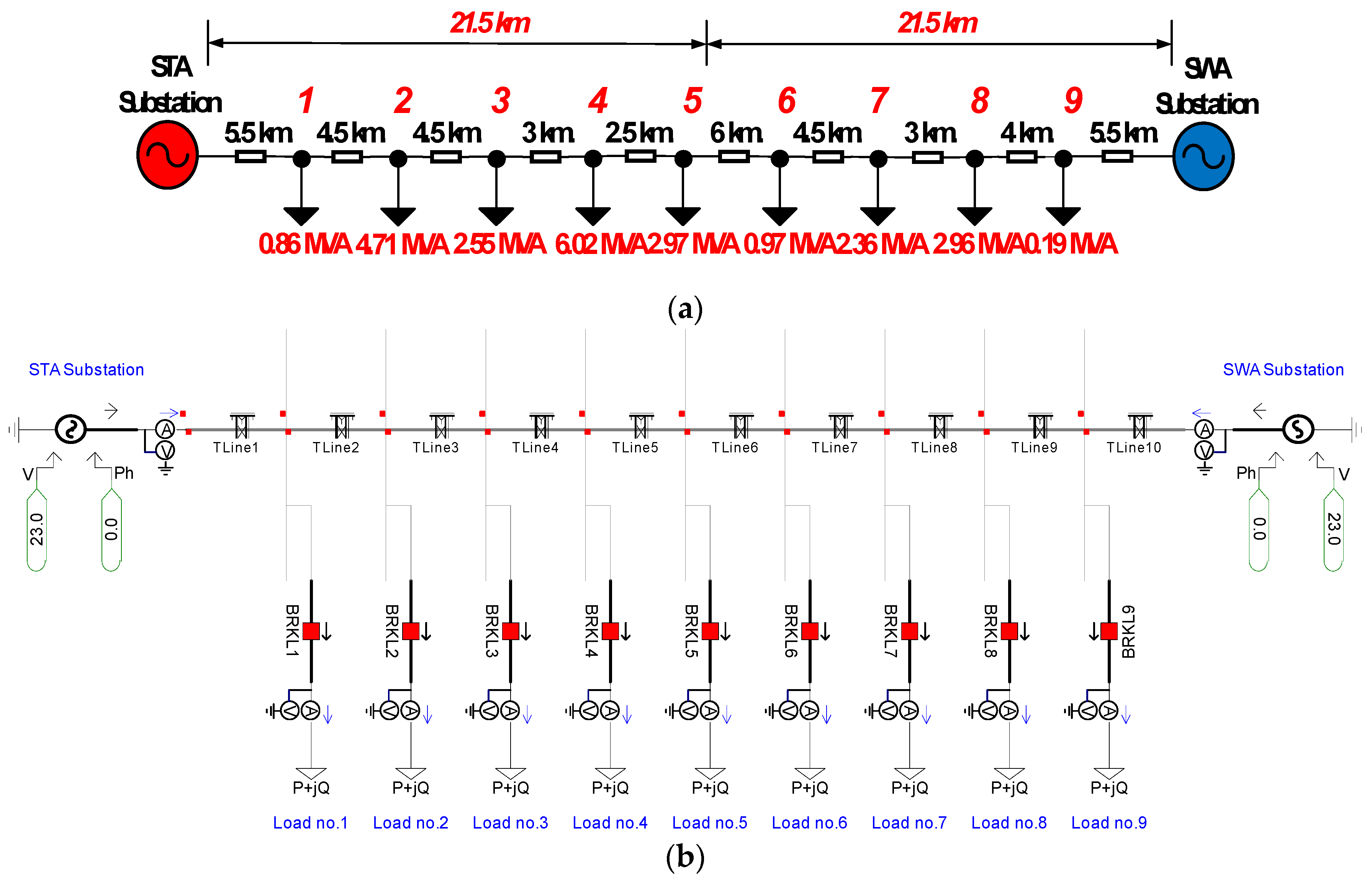
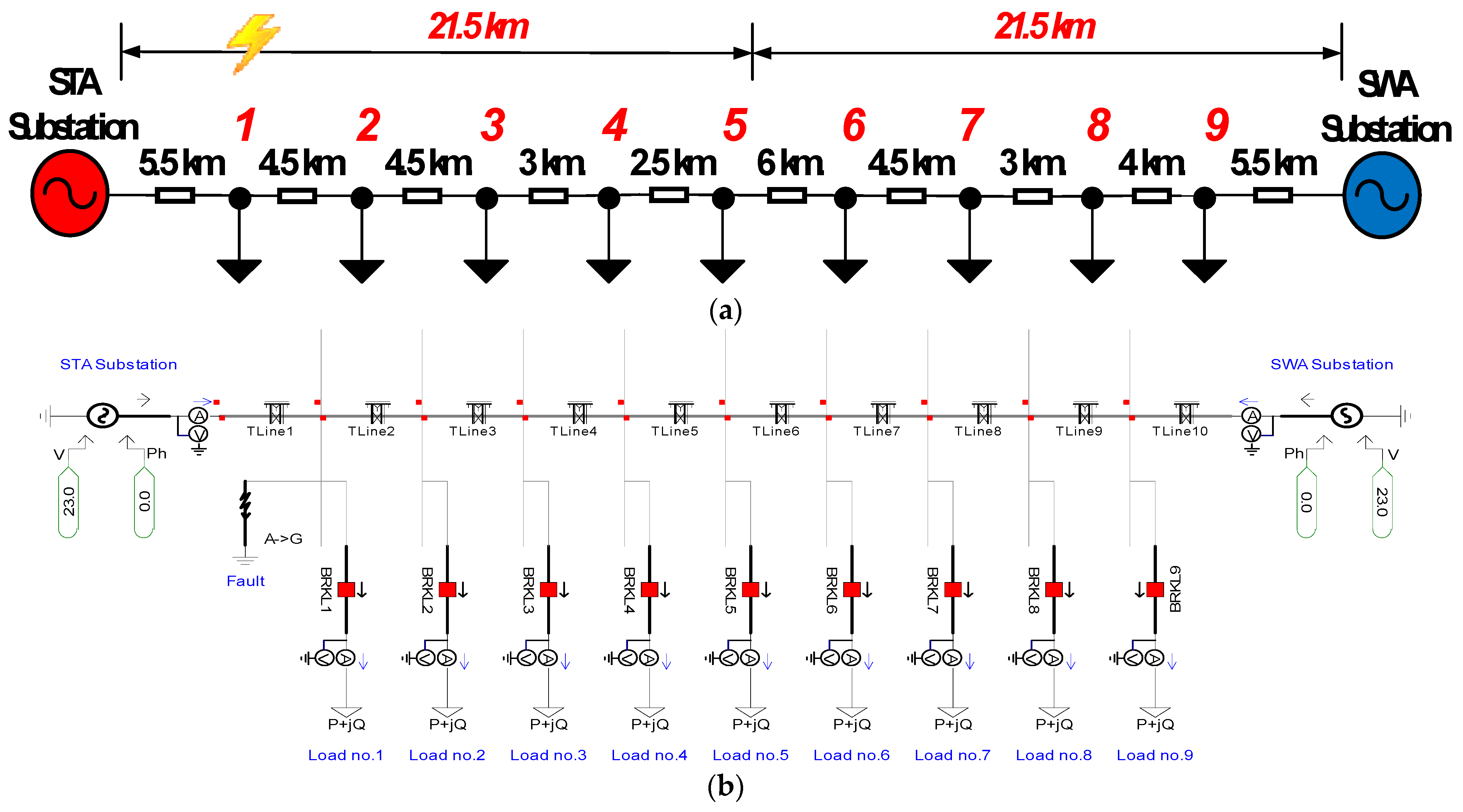
- The case study replicated an actual distribution line from the Provincial Electricity Authority (PEA) 22 kV distribution network, which represents real load and connection;
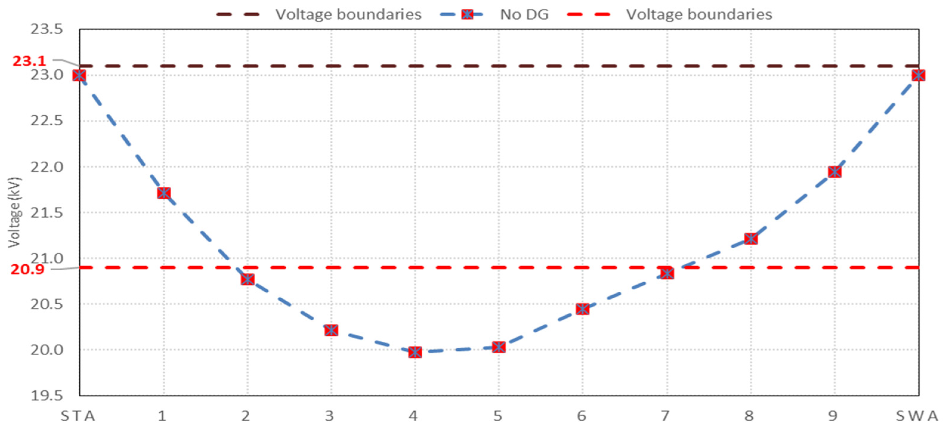
- The voltage characteristic under a normal condition and the side benefits of DG installation on the distribution in terms of voltage drop improvement were analyzed using various DG sizes, numbers, and locations;
- The current characteristic of the distribution system with various cases of DG installations under fault occurrences were also observed.
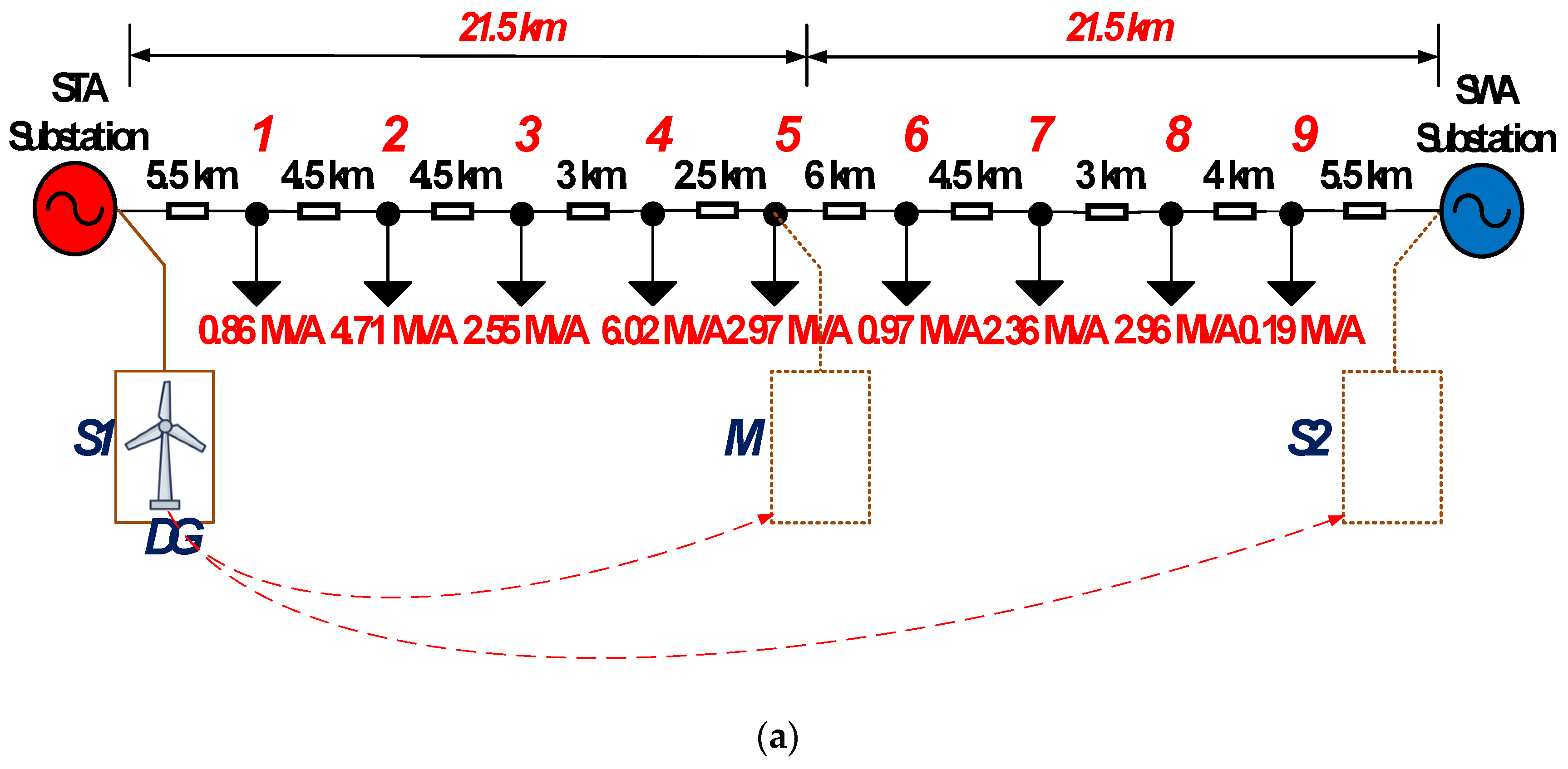
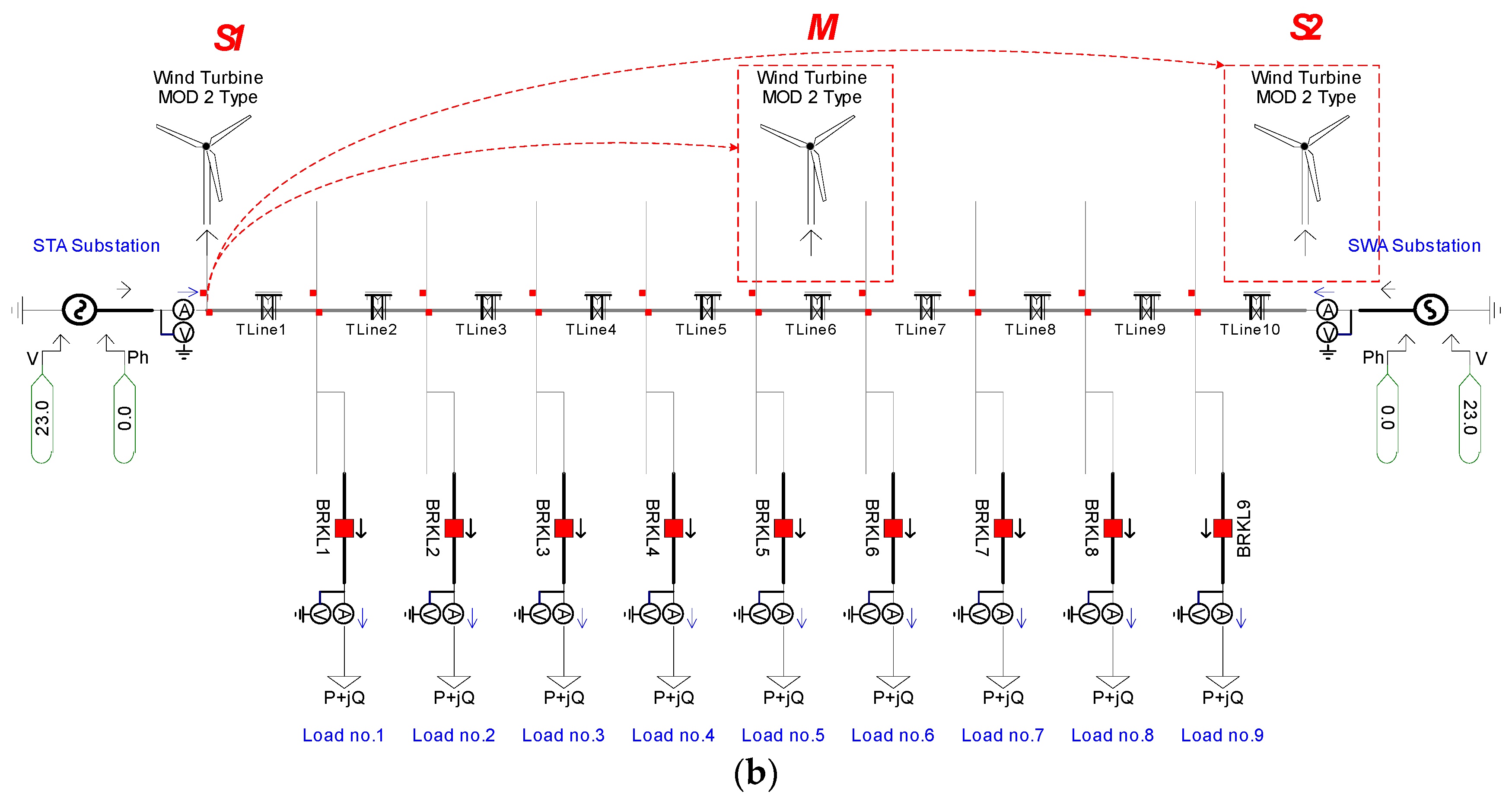
2. Case Study Distribution System
3. Distribution System with Distributed Generation
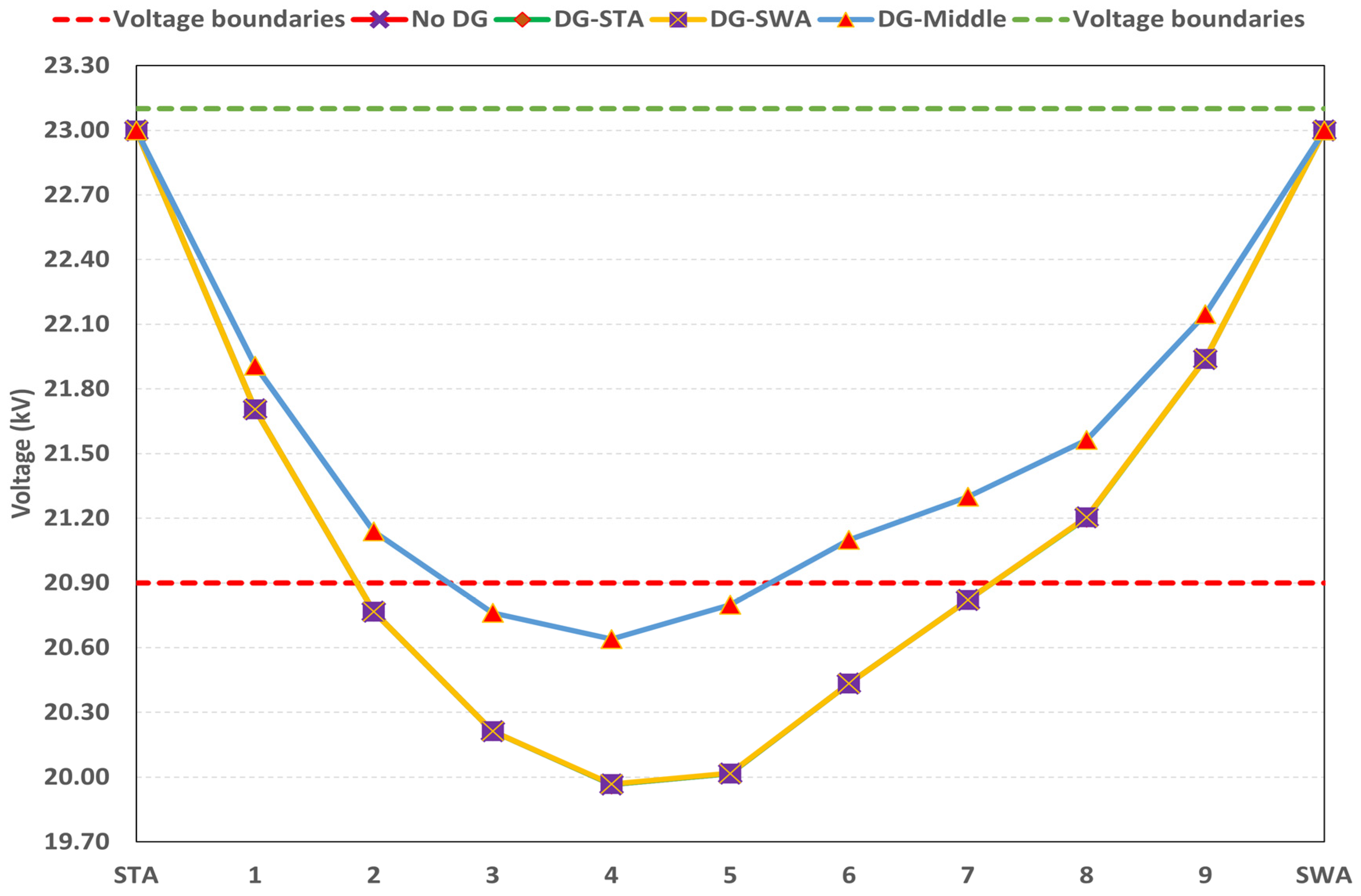
3.1. Distribution Characteristics in the Case of a Single 2 MW DG with Different Placement
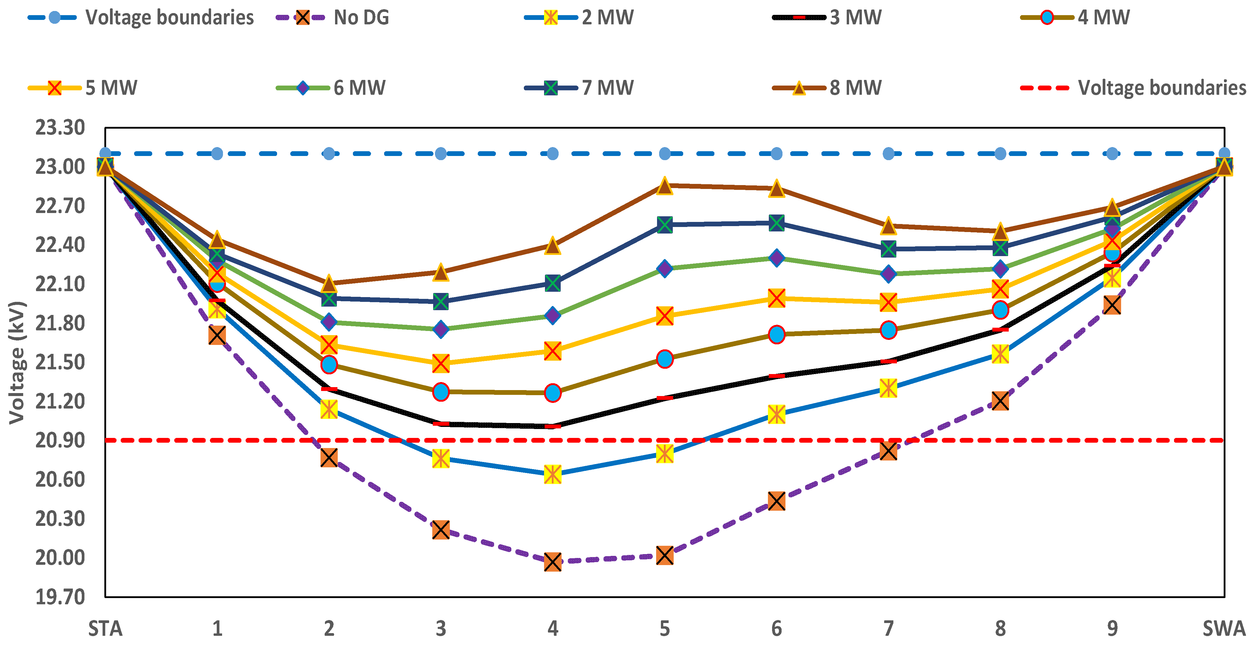
3.2. Characteristics of Voltages in the Case of Varying DG Sizing
4. Distribution System with Distributed Generation in the Case of Fault Occurrence
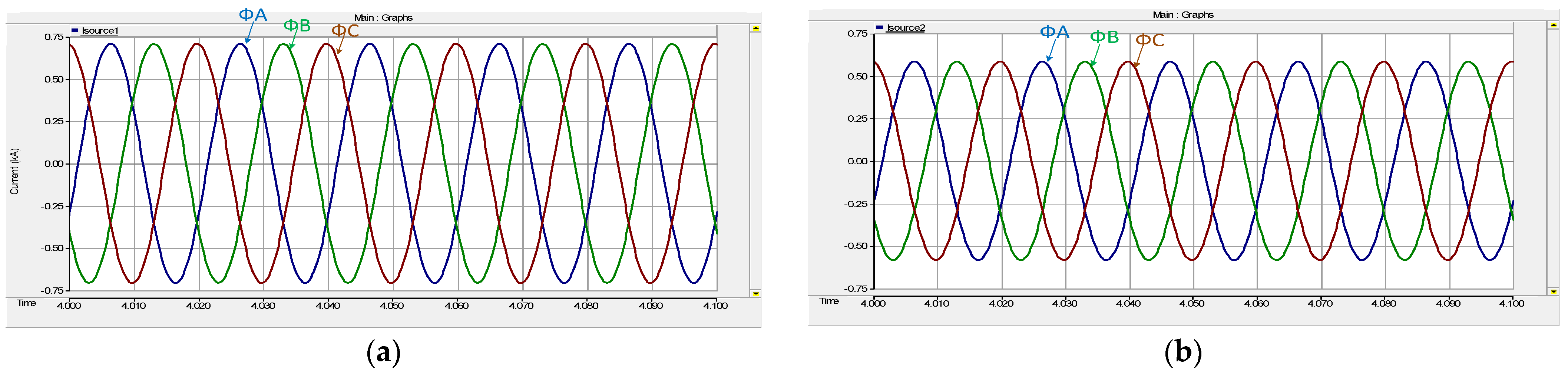
4.1. Distribution System in the Case without dg under Fault Conditions
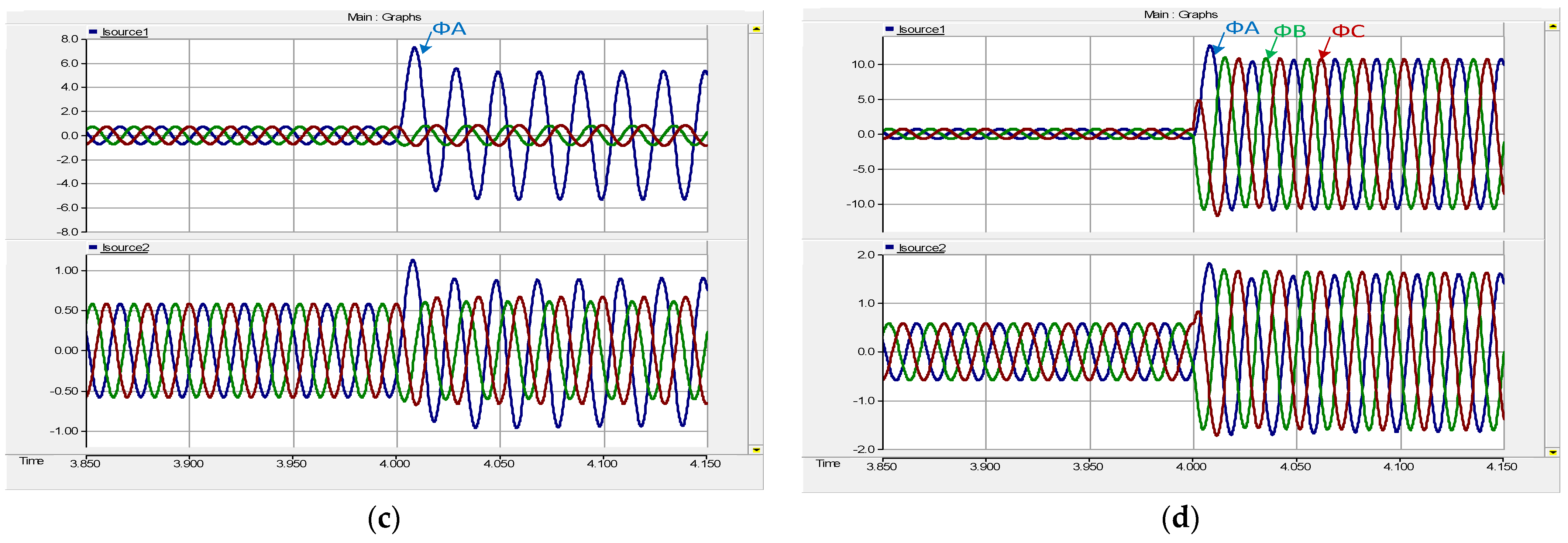
4.2. Distribution System in the Case of Single DG under Fault Conditions
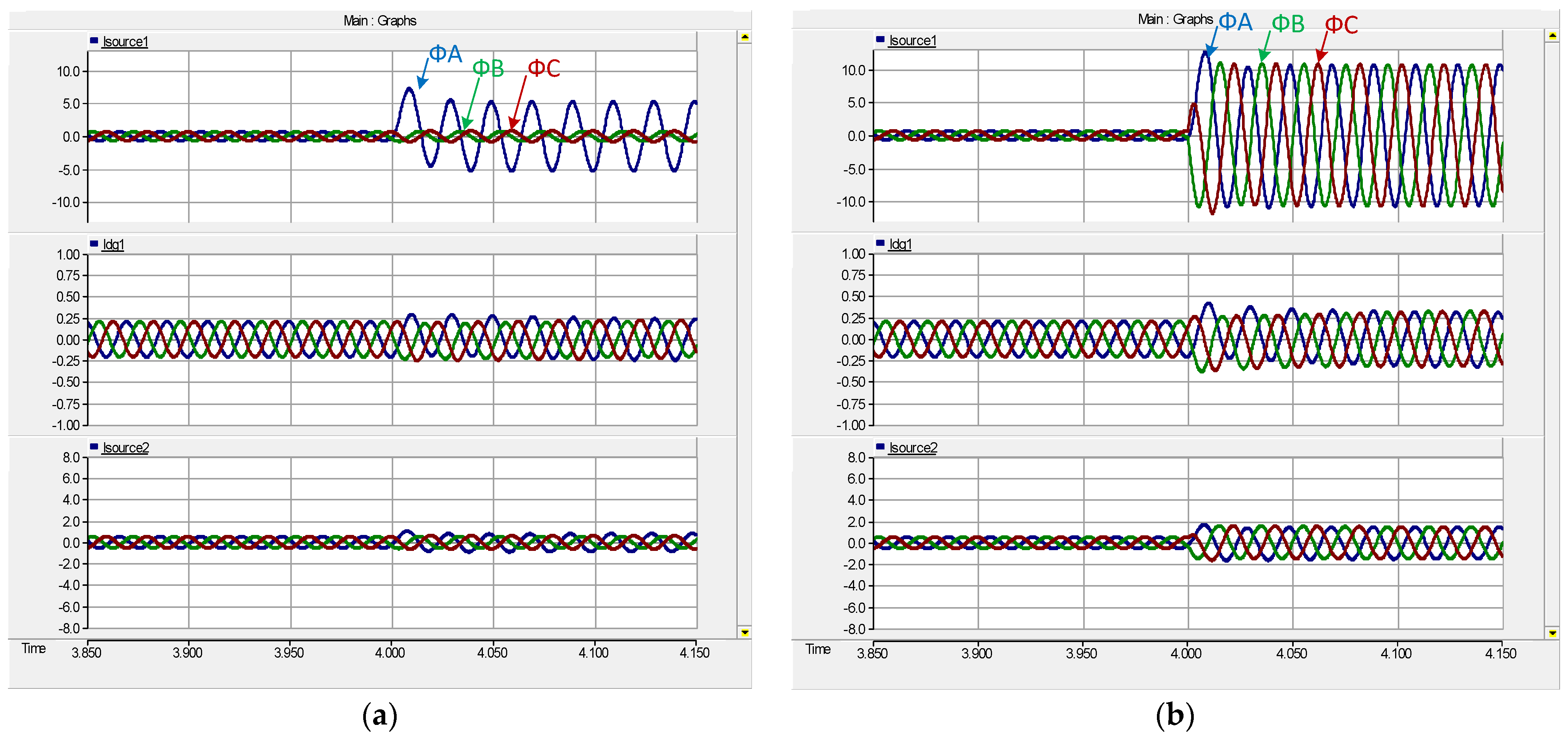
4.3. Distribution System in the Case of Single DG under Various Fault Locations
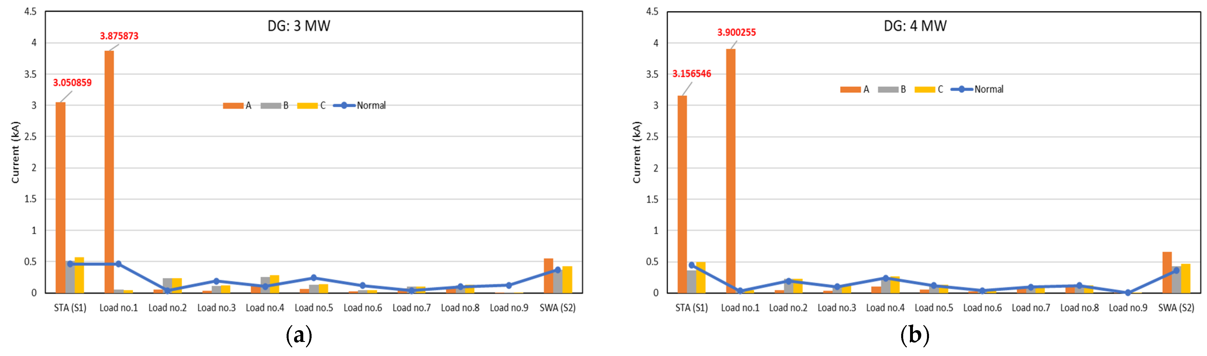
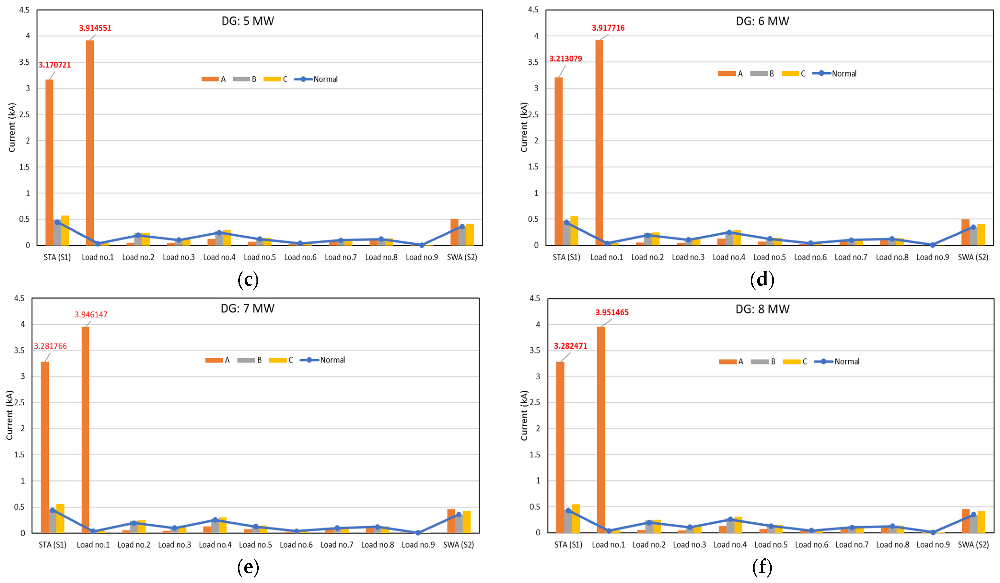
4.4. Distribution System in the Case of Various Single DG Sizing under Fault Conditions
5. Conclusions
Author Contributions
Funding
Institutional Review Board Statement
Informed Consent Statement
Data Availability Statement
Acknowledgments
Conflicts of Interest
References
- Sanamehreen, M.; Binal, M.; Divyesh, M. Grid Integration of Distributed Generation: Issues and Challenges. In Proceedings of the 2022 International Conference for Advancement in Technology (ICONAT), Goa, India, 21–22 January 2022; pp. 1–6. [Google Scholar]
- Ministry of Energy. Thailand Power Development Plan 2018–2037 (PDP 2018 Revision 1); Ministry of Energy: Bangkok, Thailand, 2020. Available online: https://www.eppo.go.th/images/Infromation_service/public_relations/PDP2018/PDP2018Rev1.pdf (accessed on 20 October 2020).
- Ministry of Energy. Alternative Energy Development Plan 2018–2037 (AEDP 2018); Ministry of Energy: Bangkok, Thailand, 2020. Available online: https://www.dede.go.th/download/Plan_62/20201021_TIEB_AEDP2018.pdf (accessed on 20 October 2020).
- Laura, M.; Deane, P.; Gallachóir, B.; Bertsch, V. A review of the role of distributed generation (DG) in future electricity systems. Energies 2018, 163, 822–836. [Google Scholar]
- Toloo, M.; Taghizadeh-Yazdi, M.; Mohammadi-Balani, A. Multi-objective centralization-decentralization trade-off analysis for multi-source renewable electricity generation expansion planning: A case study of Iran. Comput. Ind. Eng. 2022, 164, 107870. [Google Scholar]
- ChithraDevi, S.A.; Lakshminarasimman, L.; Balamurugan, R. Stud Krill herd Algorithm for multiple DG placement and sizing in a radial distribution system. Eng. Sci. Technol. Int. J. 2017, 20, 748–759. [Google Scholar] [CrossRef] [Green Version]
- Nawaz, S.; Tandon, A. A New Technique to Solve Dg Allocation Problem for Distribution Power Loss Minimization. ICIC Express Lett. Part B Appl. Int. J. Res. Surv. 2018, 9, 701–706. [Google Scholar]
- Alok, K.B.; Venkataramana, A. Investigation of Relevant Distribution System Representation with DG for Voltage Stability Margin Assessment. IEEE Trans. Power Syst. 2020, 35, 2072–2081. [Google Scholar]
- Suresh, M.C.V.; Edward, J.B. A hybrid algorithm based optimal placement of DG units for loss reduction in the distribution system. Appl. Soft Comput. 2020, 91, 106191. [Google Scholar] [CrossRef]
- Muhammad, M.A.; Chuangxin, G.; Muhammad, S.S.; Munsif, A.J.; Caiming, Y.; Jianguang, Z. A Review of Technical Methods for Distributed Systems with Distributed Generation (DG). In Proceedings of the 2019 2nd International Conference on Computing, Mathematics and Engineering Technologies (iCoMET), Sukkur, Pakistan, 30–31 January 2019; pp. 1–7. [Google Scholar]
- Iqbal, F.; Khan, M.T.; Siddiqui, A.S. Optimal placement of DG and DSTATCOM for loss reduction and voltage profile improvement. Alex. Eng. J. 2018, 57, 755–765. [Google Scholar]
- Pankita, M.; Praghnesh, B.; Vivek, P. Optimal selection of distributed generating units and its placement for voltage stability enhancement and energy loss minimization. Ain Shams Eng. J. 2018, 9, 187–201. [Google Scholar]
- Paschalis, A.G.; Aggelos, S.B.; Dimitrios, I.D.; Kallisthenis, I.S.; Dimitris, P.L. Load variations impact on optimal DG placement problem concerning energy loss reduction. Electr. Power Syst. Res. 2017, 152, 36–47. [Google Scholar]
- Haijun, X.; Xin, S. Distributed Generation Locating and Sizing in Active Distribution Network Considering Network Reconfiguration. IEEE Access. 2017, 5, 14768–14774. [Google Scholar]
- Sirine, E.; Adel, B.; Adel., K. Optimal Sizing and Placement of DG Units in Radial Distribution System. Int. J. Renew. Energy Res. 2018, 8, 167–177. [Google Scholar]
- Alwash, S.F.; Ramachandaramurthy, V.K.; Mithulananthan, N. Fault-Location Scheme for Power Distribution System with Distributed Generation. IEEE Trans. Power Deliv. 2015, 30, 1187–1195. [Google Scholar] [CrossRef] [Green Version]
- Mohsin, S.; Waseem, A.; Muhammad, A.; Uzair, K.; Barkat, U. Optimal Siting and Sizing of Distributed Generators by Strawberry Plant Propagation Algorithm. Energies 2021, 14, 3–13. [Google Scholar]
- Ali, T.; Faissal, E.; Abdelaziz, B.; Touria, H.; Naima, A.; Rabiaa, G. Meta-heuristics Applied to Multiple DG Allocation in Radial Distribution Network: A comparative study. In Proceedings of the 2022 International Conference on Intelligent Systems and Computer Vision (ISCV), Fez, Morocco, 18–20 May 2022; pp. 1–8. [Google Scholar]
- Mohammad, I.; Mohsin, S.; Noman, U. Analytical Method for Optimal Reactive Power Support in Power Network. In Proceedings of the 2019 2nd International Conference on Computing, Mathematics and Engineering Technologies (iCoMET), Sukkur, Pakistan, 30–31 January 2019; pp. 1–6. [Google Scholar]
- Chiradeja, P.; Yoomak, S.; Ngaopitakkul, A. The study of economic effects when different distributed generators (DG) connected to a distribution system. In Proceedings of the 2018 19th International Scientific Conference on Electric Power Engineering (EPE), Brno, Czech Republic, 16–18 May 2018; pp. 1–5. [Google Scholar]
- Ngaopitakkul, A.; Jettanasen, C. The effects of multi-distributed generator on distribution system reliability. In Proceedings of the 2017 IEEE Innovative Smart Grid Technologies—Asia (ISGT-Asia), Auckland, New Zealand, 4–7 December 2017; pp. 1–6. [Google Scholar]
- Hany, F.H.; Nevin, F.; Mohammad, M.E.; Osama, A.M. Enhancement of Protection Scheme for Distribution System Using the Communication Network. In Proceedings of the 2019 IEEE Industry Applications Society Annual Meeting, Baltimore, MD, USA, 29 September–3 October 2019; pp. 2–7. [Google Scholar]
- Digambar, R.B.; Ravishankar, S.K.; Saurabh, J. Impact of Distributed Generation on Protection of Power System. In Proceedings of the 2017 International Conference on Innovative Mechanisms for Industry Applications (ICIMIA), Bengaluru, India, 21–23 February 2017; pp. 399–405. [Google Scholar]
- Langlang, G.; Muhammad, A.H.; Mokhammad, S.; Wahyu, S.N. Analysis of Short Circuit on Four Types Wind Power Plants as Distributed Generation. In Proceedings of the 2020 International Conference on Smart Technology and Applications (ICoSTA), Surabaya, Indonesia, 20 February 2020; pp. 1–6. [Google Scholar]
- Mehdi, M.; Matin, M.; Abbas, F. Impact of Size and Location of Distributed Generation on Overcurrent Relays in Active Distribution Networks. In Proceedings of the 2017 North American Power Symposium (NAPS), Morgantown, WV, USA, 17–19 September 2017; pp. 1–6. [Google Scholar]
- Reza, M.C.; Ehsan, M.H.; Meysam, F. The effect of fault current limiter size and type on current limitation in the presence of distributed generation. Turk. J. Electr. Eng. Comput. Sci. 2017, 25, 1021–1034. [Google Scholar]
- Adel, A.A.E.; Ragab, A.E.; Abdullah, M.S.; Aya, R.E. Optimal Allocation of Distributed Generation Units Correlated with Fault Current Limiter Sites in Distribution Systems. IEEE Syst. J. 2021, 15, 2148–2155. [Google Scholar]
- Mir, E.H.; Reza, M.C. Optimal Allocation of Distributed Generation with Optimal Sizing of Fault Current Limiter to Reduce the Impact on Distribution Networks Using NSGA-II. IEEE Syst. J. 2019, 13, 1714–1724. [Google Scholar]
- Matin, M.; Alexander, D.; Ilya, G. Impact of distributed generation on the protection systems of distribution networks: Analysis and remedies–Review paper. IET Gener. Transm. Distrib. 2020, 14, 5944–5960. [Google Scholar]
- Ayoade, F.A.; Owolabi, B.; Ademola, A.; Ayokunle, A.; Tobiloba, S.; Akinola, O.; Agbetuyi, O. Investigation of the Impact of Distributed Generation on Power System Protection. Adv. Sci. Technol. Eng. Syst. J. 2021, 6, 324–331. [Google Scholar]
- Hamid, M.; Rahman, D.; Ahmad, K.; Amin, J.T.; Hamid, R.S. A Novel Fault Location Methodology for Smart Distribution Networks. IEEE Trans. Smart Grid 2021, 12, 1277–1288. [Google Scholar]
- Gustavo, G.S.; José Carlos, M.V. Optimal Placement of Fault Indicators to Identify Fault Zones in Distribution Systems. IEEE Trans. Power Deliv. 2021, 36, 3282–3285. [Google Scholar]
- Haotian, S.; Hao, Y.; Fang, Z.; Xiaotong, D.; Guangyu, Y. Precise Fault Location in Distribution Networks Based on Optimal Monitor Allocation. IEEE Trans. Power Deliv. 2020, 35, 1788–1799. [Google Scholar]
- Farzaneh, S.; Mohammad, R.; Morteza, D. Simultaneous Placement of Tie-lines and Distributed Generations to Optimize Distribution System Post-Outage Operations and Minimize Energy Losses. CSEE J. Power Energy Syst. 2021, 7, 318–328. [Google Scholar]
- Liuzhu, Z.; Bin, Y.; Xijun, R.; Bao, W.; Xiaoyu, S.; Mao, Z.; Pei, Z.; Xiaoxi, L.; Jiateng, L. Transmission Pricing for Distributed Generation Transactions Based on Cost and Benefit Analysis. In Proceedings of the 2020 IEEE 4th Conference on Energy Internet and Energy System Integration (EI2), Wuhan, China, 30 October–1 November 2020; pp. 4397–4402. [Google Scholar]
- Bangun, N.; Kamaruddin, A.; Aep, S.U.; Erkata, Y.; Syukri, M.N.; Herry, S.; Zane, V.; Roy, H.S.; Yanuar, N. Smart Micro-Grid Performance using Renewable Energy. ICESTI 2019, 188, 1–11. [Google Scholar]


| Parameters | Configurations |
|---|---|
| 1. Rated voltage (VL-L, Vrms) | 22 kV |
| 2. Boundary voltage | 20.9–23.1 kV |
| 3. Lean conductor | 3 conductors |
| ▪ SAC cable | 185 mm2 |
| ▪ Outer diameter | 0.00799 m |
| ▪ DC resistance | 0.164 Ω |
| 4. Distribution line length | 43 km |
| 5. Total loads | 9 loads |
| 6. PF loads | 0.95 |
| Load No. | Distance (STA–Load) (km) | Apparent Power (MVA) | PF. |
|---|---|---|---|
| 1 | 5.5 | 0.86 | 0.95 |
| 2 | 10 | 4.71 | 0.95 |
| 3 | 14.5 | 2.55 | 0.95 |
| 4 | 17.5 | 6.02 | 0.95 |
| 5 | 20 | 2.97 | 0.95 |
| 6 | 26 | 0.97 | 0.95 |
| 7 | 30.5 | 2.36 | 0.95 |
| 8 | 33.5 | 2.96 | 0.95 |
| 9 | 37.5 | 0.19 | 0.95 |
| 23.59 MVA |
| Descriptions | Parameters Recorded | |||||
|---|---|---|---|---|---|---|
| V (kV) | I (kA) | P (MW) | Q (MVAr) | S (MVA) | ||
| Measuring Points | STA (S1) | 23.000000 | 0.499433 | 19.174202 | 8.096472 | 20.813526 |
| Load No. 1 | 21.705532 | 0.035279 | 1.255549 | 0.427419 | 1.326307 | |
| Load No. 2 | 20.766570 | 0.184679 | 6.308891 | 2.078501 | 6.642459 | |
| Load No. 3 | 20.213322 | 0.097514 | 3.243475 | 1.065713 | 3.414070 | |
| Load No. 4 | 19.967074 | 0.226968 | 7.460242 | 2.441514 | 7.849598 | |
| Load No. 5 | 20.017326 | 0.112525 | 3.703464 | 1.226886 | 3.901396 | |
| Load No. 6 | 20.433511 | 0.037232 | 1.254766 | 0.402474 | 1.317734 | |
| Load No. 7 | 20.821111 | 0.093333 | 3.195578 | 1.056986 | 3.365848 | |
| Load No. 8 | 21.203214 | 0.118314 | 4.129579 | 1.351087 | 4.344980 | |
| Load No. 9 | 21.939189 | 0.007498 | 0.272923 | 0.081175 | 0.284739 | |
| SWA (S2) | 23.000000 | 0.413103 | 15.078666 | 6.592662 | 16.456894 | |
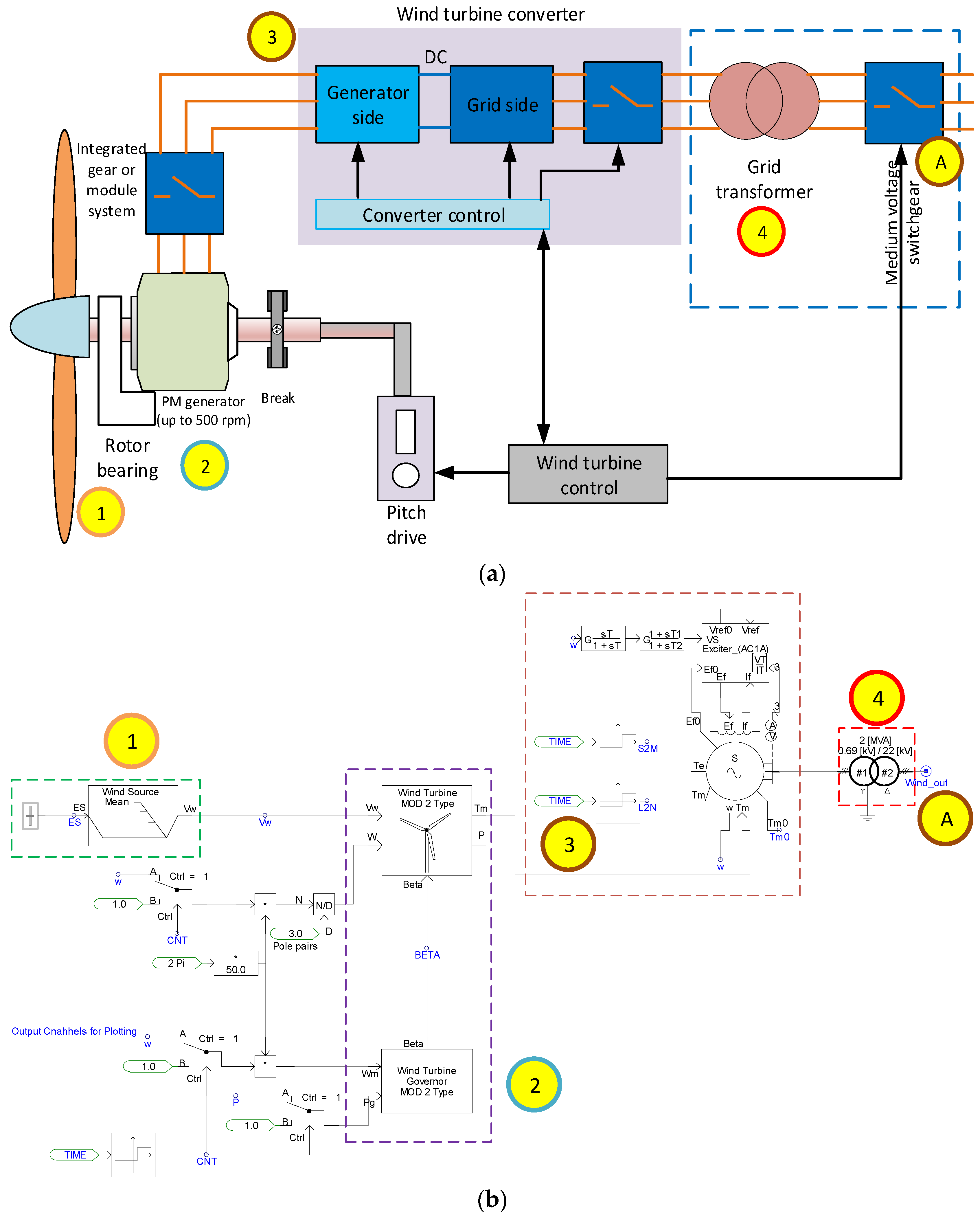
| Components | Parameters | Configurations |
|---|---|---|
| 1. Wind Source | Average wind Speed (m/s) | 6 |
| 2. Wind Turbine Generator | Generator rated (MVA) | 2 |
| Rotor radius (m) | 43.5 | |
| Rotor area (m2) | 5944 | |
| Air density (kg/m3) | 1.225 | |
| 3. Synchronous Machine | Rate voltage per phase (kV) | 0.398 |
| Rate current (kA) | 1.840 | |
| Frequency (Hz) | 50 | |
| 4. Unit Transformer | Frequency (Hz) | 50 |
| Apparent power (MVA) | 2 | |
| Primary voltage (kV) | 0.690 | |
| Secondary voltage (kV) | 22 |
| Items | Measuring Points | Descriptions | |||||||
|---|---|---|---|---|---|---|---|---|---|
| Base Case (No DG) | Near STA Substation (DG-STA) | On the Middle Point of the Distribution Line (DG-Middle) | Near SWA Substation (DG-SWA) | Base Case (No DG) | Near STA Substation (DG-STA) | On the Middle Point of the Distribution Line (DG-Middle) | Near SWA Substation (DG-SWA) | ||
| Voltage (kV) | Current (kA) | ||||||||
| 1 | STA (S1) | 23.000000 | 23.000000 | 23.000000 | 23.000000 | 0.499433 | 0.411413 | 0.468915 | 0.499443 |
| 2 | Load No. 1 | 21.705532 | 21.705543 | 21.908088 | 21.705561 | 0.035279 | 0.035279 | 0.035607 | 0.035279 |
| 3 | Load No. 2 | 20.766570 | 20.766675 | 21.138453 | 20.766642 | 0.184679 | 0.184673 | 0.187696 | 0.184673 |
| 4 | Load No. 3 | 20.213322 | 20.213380 | 20.761723 | 20.213555 | 0.097514 | 0.097515 | 0.100147 | 0.097515 |
| 5 | Load No. 4 | 19.967074 | 19.967146 | 20.639817 | 19.967360 | 0.226968 | 0.226969 | 0.234555 | 0.226972 |
| 6 | Load No. 5 | 20.017326 | 20.017389 | 20.798338 | 20.017638 | 0.112525 | 0.112525 | 0.116922 | 0.112526 |
| 7 | Load No. 6 | 20.433511 | 20.433512 | 21.099504 | 20.433847 | 0.037232 | 0.037232 | 0.038440 | 0.037233 |
| 8 | Load No. 7 | 20.821111 | 20.821148 | 21.300304 | 20.821548 | 0.093333 | 0.093333 | 0.095484 | 0.093335 |
| 9 | Load No. 8 | 21.203214 | 21.203240 | 21.563076 | 21.203488 | 0.118314 | 0.118314 | 0.120318 | 0.118316 |
| 10 | Load No. 9 | 21.939189 | 21.939206 | 22.146445 | 21.939720 | 0.007498 | 0.007498 | 0.007569 | 0.007498 |
| 11 | SWA (S2) | 23.000000 | 23.000000 | 23.000000 | 23.000000 | 0.413103 | 0.413099 | 0.381220 | 0.330026 |
| Single DG Sizing | Measuring Points | ||||||||||
|---|---|---|---|---|---|---|---|---|---|---|---|
| STA | 1 | 2 | 3 | 4 | 5 | 6 | 7 | 8 | 9 | SWA | |
| no DG | 23.000000 | 21.705532 | 20.766570 | 20.213322 | 19.967074 | 20.017326 | 20.433511 | 20.821111 | 21.203214 | 21.939189 | 23.000000 |
| 2 MW | 23.000000 | 21.908088 | 21.138453 | 20.761723 | 20.639817 | 20.798338 | 21.099504 | 21.300304 | 21.563076 | 22.146445 | 23.000000 |
| 3 MW | 23.000000 | 21.974048 | 21.293040 | 21.025706 | 21.006142 | 21.222554 | 21.392216 | 21.504872 | 21.748671 | 22.239908 | 23.000000 |
| 4 MW | 23.000000 | 22.107511 | 21.482672 | 21.272889 | 21.265034 | 21.525231 | 21.713015 | 21.746262 | 21.901710 | 22.342198 | 23.000000 |
| 5 MW | 23.000000 | 22.184035 | 21.632193 | 21.489586 | 21.586236 | 21.854500 | 21.990732 | 21.959655 | 22.061591 | 22.433231 | 23.000000 |
| 6 MW | 23.000000 | 22.281338 | 21.807338 | 21.751126 | 21.856676 | 22.217459 | 22.299483 | 22.176007 | 22.216389 | 22.524413 | 23.000000 |
| 7 MW | 23.000000 | 22.333308 | 21.990926 | 21.964674 | 22.105478 | 22.554267 | 22.567886 | 22.367582 | 22.380118 | 22.614138 | 23.000000 |
| 8 MW | 23.000000 | 22.441116 | 22.105417 | 22.191798 | 22.397389 | 22.855555 | 22.834169 | 22.547406 | 22.504952 | 22.688590 | 23.000000 |
| Fault Location | Parameters | Measuring Points | |||||||||||
|---|---|---|---|---|---|---|---|---|---|---|---|---|---|
| STA (S1) | Load No. 1 | Load No. 2 | Load No. 3 | Load No. 4 | Load No. 5 | Load No. 6 | Load No. 7 | Load No. 8 | Load No. 9 | SWA (S2) | |||
| Normal Condition | RMS current (kA) | A | 0.499433 | 0.035279 | 0.184679 | 0.097514 | 0.226968 | 0.112525 | 0.037232 | 0.093333 | 0.118314 | 0.007498 | 0.413103 |
| B | 0.499433 | 0.035279 | 0.184679 | 0.097514 | 0.226968 | 0.112525 | 0.037232 | 0.093333 | 0.118314 | 0.007498 | 0.413103 | ||
| C | 0.499433 | 0.035279 | 0.184679 | 0.097514 | 0.226968 | 0.112525 | 0.037232 | 0.093333 | 0.118314 | 0.007498 | 0.413103 | ||
| Fault at 5.5 km (L1) | RMS current (kA) | A | 3.425437 | 3.80059 | 0.045354 | 0.034836 | 0.104118 | 0.059266 | 0.025076 | 0.072426 | 0.098934 | 0.006807 | 0.656846 |
| B | 0.570717 | 0.048403 | 0.227256 | 0.110387 | 0.244291 | 0.118632 | 0.037849 | 0.093260 | 0.11784 | 0.00748 | 0.431361 | ||
| C | 0.60103 | 0.045938 | 0.231498 | 0.118328 | 0.270682 | 0.131697 | 0.041878 | 0.101779 | 0.1262 | 0.00778 | 0.470331 | ||
| Fault at 10 km (L2) | RMS current (kA) | A | 2.039706 | 0.018407 | 2.534366 | 0.025607 | 0.075196 | 0.046396 | 0.022077 | 0.067126 | 0.094045 | 0.006635 | 0.736406 |
| B | 0.584159 | 0.040447 | 0.242797 | 0.115761 | 0.253281 | 0.122223 | 0.038493 | 0.094094 | 0.118467 | 0.007506 | 0.444318 | ||
| C | 0.612174 | 0.040432 | 0.239505 | 0.12189 | 0.278379 | 0.135086 | 0.04227 | 0.103318 | 0.127651 | 0.007829 | 0.479773 | ||
| Fault at 17.5 km (L3) | RMS current (kA) | A | 1.28695 | 0.02593 | 0.092053 | 0.031512 | 1.979025 | 0.031697 | 0.015228 | 0.05431 | 0.081949 | 0.006207 | 0.920934 |
| B | 0.576755 | 0.036578 | 0.200288 | 0.11494 | 0.287371 | 0.136297 | 0.041345 | 0.098378 | 0.122088 | 0.007624 | 0.462517 | ||
| C | 0.607462 | 0.038518 | 0.21505 | 0.121232 | 0.294322 | 0.141964 | 0.044407 | 0.106478 | 0.130603 | 0.007931 | 0.490508 | ||
| Fault at 20 km (L4) | RMS Current (kA) | A | 1.144118 | 0.027471 | 0.107245 | 0.035007 | 0.056589 | 1.880047 | 0.014092 | 0.049399 | 0.076969 | 0.006017 | 0.990623 |
| B | 0.562203 | 0.036117 | 0.195049 | 0.109855 | 0.27104 | 0.14385 | 0.042907 | 0.100751 | 0.124109 | 0.007693 | 0.46411 | ||
| C | 0.598486 | 0.037899 | 0.21074 | 0.117767 | 0.28416 | 0.14591 | 0.045309 | 0.108073 | 0.132065 | 0.00798 | 0.489472 | ||
| Fault at 33.5 km (L5) | RMS Current (kA) | A | 0.786051 | 0.031503 | 0.146545 | 0.066019 | 0.133924 | 0.057004 | 0.011675 | 0.026774 | 2.513962 | 0.003605 | 2.065382 |
| B | 0.527778 | 0.035217 | 0.184619 | 0.099259 | 0.236191 | 0.12059 | 0.044063 | 0.118574 | 0.158727 | 0.008857 | 0.474618 | ||
| C | 0.56739 | 0.036791 | 0.199489 | 0.10909 | 0.259745 | 0.131519 | 0.045305 | 0.118059 | 0.154326 | 0.00866 | 0.488163 | ||
| Fault at 37.5 km (L6) | RMS current (kA) | A | 0.728949 | 0.032086 | 0.152416 | 0.07073 | 0.147694 | 0.065068 | 0.014511 | 0.025329 | 0.028757 | 3.713365 | 3.355621 |
| B | 0.518104 | 0.035196 | 0.184339 | 0.0987 | 0.233933 | 0.118883 | 0.042851 | 0.114254 | 0.151947 | 0.101409 | 0.469314 | ||
| C | 0.558022 | 0.036599 | 0.197586 | 0.107615 | 0.255573 | 0.129131 | 0.044292 | 0.114906 | 0.149521 | 0.009837 | 0.481258 | ||
| Fault Location | Parameters | Measuring Points | |||||||||||
|---|---|---|---|---|---|---|---|---|---|---|---|---|---|
| STA (S1) | Load No. 1 | Load No. 2 | Load No. 3 | Load No. 4 | Load No. 5 | Load No. 6 | Load No. 7 | Load No. 8 | Load No. 9 | SWA (S2) | |||
| Normal Condition | RMS Current (kA) | A | 0.462155 | 0.035898 | 0.190778 | 0.102424 | 0.241254 | 0.120776 | 0.039484 | 0.097338 | 0.122070 | 0.007628 | 0.372955 |
| B | 0.462155 | 0.035898 | 0.190778 | 0.102424 | 0.241254 | 0.120776 | 0.039484 | 0.097338 | 0.122070 | 0.007628 | 0.372955 | ||
| C | 0.462155 | 0.035898 | 0.190778 | 0.102424 | 0.241254 | 0.120776 | 0.039484 | 0.097338 | 0.122070 | 0.007628 | 0.372955 | ||
| Fault at 5.5 km (L1) | RMS Current (kA) | A | 3.350859 | 3.875873 | 0.049368 | 0.039561 | 0.117352 | 0.067317 | 0.027353 | 0.076529 | 0.102934 | 0.006947 | 0.550503 |
| B | 0.509782 | 0.049651 | 0.234932 | 0.115791 | 0.259409 | 0.127304 | 0.040195 | 0.097321 | 0.121592 | 0.007610 | 0.373297 | ||
| C | 0.569199 | 0.046875 | 0.239042 | 0.124110 | 0.287262 | 0.140970 | 0.044451 | 0.106379 | 0.130555 | 0.007932 | 0.428855 | ||
| Fault at 10 km (L2) | RMS Current (kA) | A | 1.969711 | 0.018456 | 2.636615 | 0.027950 | 0.086082 | 0.053203 | 0.024157 | 0.070917 | 0.097640 | 0.006758 | 0.630972 |
| B | 0.520884 | 0.041206 | 0.251161 | 0.121614 | 0.268988 | 0.131079 | 0.040847 | 0.098137 | 0.122272 | 0.007629 | 0.389854 | ||
| C | 0.591338 | 0.041413 | 0.249009 | 0.128351 | 0.296177 | 0.145131 | 0.045448 | 0.108213 | 0.132329 | 0.007991 | 0.441544 | ||
| Fault at 17.5 km (L3) | RMS Current (kA) | A | 1.218242 | 0.025997 | 0.092901 | 0.032938 | 2.142779 | 0.027515 | 0.015812 | 0.056099 | 0.083815 | 0.006267 | 0.829761 |
| B | 0.519040 | 0.037207 | 0.207318 | 0.121206 | 0.307445 | 0.146750 | 0.043992 | 0.102758 | 0.126037 | 0.007755 | 0.410029 | ||
| C | 0.583505 | 0.030340 | 0.225305 | 0.129308 | 0.317921 | 0.154032 | 0.047724 | 0.112414 | 0.136087 | 0.008125 | 0.458019 | ||
| Fault at 20 km (L4) | RMS Current (kA) | A | 1.217067 | 0.025970 | 0.092311 | 0.032283 | 2.141804 | 0.026847 | 0.015756 | 0.056206 | 0.083878 | 0.006265 | 0.828898 |
| B | 0.522745 | 0.037207 | 0.207329 | 0.121361 | 0.306798 | 0.146636 | 0.044006 | 0.102680 | 0.126119 | 0.007755 | 0.407454 | ||
| C | 0.587915 | 0.039346 | 0.225305 | 0.129355 | 0.317864 | 0.154004 | 0.047727 | 0.112475 | 0.136128 | 0.008128 | 0.460042 | ||
| Fault at 33.5 km (L5) | RMS Current (kA) | A | 0.694390 | 0.031997 | 0.151590 | 0.069843 | 0.144844 | 0.063071 | 0.012523 | 0.028027 | 0.053128 | 0.003845 | 1.889275 |
| B | 0.476797 | 0.035832 | 0.191145 | 0.104663 | 0.252375 | 0.130098 | 0.047069 | 0.125118 | 0.160301 | 0.008902 | 0.412728 | ||
| C | 0.530858 | 0.037564 | 0.207296 | 0.115419 | 0.277644 | 0.141896 | 0.048297 | 0.124230 | 0.158084 | 0.008812 | 0.466108 | ||
| Fault at 37.5 km (L6) | RMS Current (kA) | A | 0.632474 | 0.032714 | 0.158713 | 0.075744 | 0.162303 | 0.073428 | 0.016677 | 0.028405 | 0.031145 | 3.790341 | 3.278373 |
| B | 0.465596 | 0.035805 | 0.190499 | 0.103811 | 0.248799 | 0.127528 | 0.045330 | 0.118906 | 0.156489 | 0.010595 | 0.410326 | ||
| C | 0.519209 | 0.037301 | 0.204732 | 0.113329 | 0.272003 | 0.138420 | 0.046848 | 0.119672 | 0.154281 | 0.010004 | 0.456568 | ||
Disclaimer/Publisher’s Note: The statements, opinions and data contained in all publications are solely those of the individual author(s) and contributor(s) and not of MDPI and/or the editor(s). MDPI and/or the editor(s) disclaim responsibility for any injury to people or property resulting from any ideas, methods, instructions or products referred to in the content. |
© 2023 by the authors. Licensee MDPI, Basel, Switzerland. This article is an open access article distributed under the terms and conditions of the Creative Commons Attribution (CC BY) license (https://creativecommons.org/licenses/by/4.0/).
Share and Cite
Ngamroo, I.; Kotesakha, W.; Yoomak, S.; Ngaopitakkul, A. Characteristic Evaluation of Wind Power Distributed Generation Sizing in Distribution System. Sustainability 2023, 15, 5581. https://doi.org/10.3390/su15065581
Ngamroo I, Kotesakha W, Yoomak S, Ngaopitakkul A. Characteristic Evaluation of Wind Power Distributed Generation Sizing in Distribution System. Sustainability. 2023; 15(6):5581. https://doi.org/10.3390/su15065581
Chicago/Turabian StyleNgamroo, Issarachai, Wikorn Kotesakha, Suntiti Yoomak, and Atthapol Ngaopitakkul. 2023. "Characteristic Evaluation of Wind Power Distributed Generation Sizing in Distribution System" Sustainability 15, no. 6: 5581. https://doi.org/10.3390/su15065581