Spatial Correlation Network Structure of Carbon Emission Efficiency in China’s Construction Industry and Its Formation Mechanism

Abstract

In the context of “carbon peak, carbon neutrality”, it is important to explore the spatial correlation network of carbon emission efficiency in the construction industry and its formation mechanism to promote regional synergistic carbon emission reduction. This paper analyzes the spatial correlation network of carbon emission efficiency in China’s construction industry and its formation mechanism through the use of the global super-efficiency EBM model, social network analysis, and QAP model. The results show that (1) the national construction industry’s overall carbon emission efficiency is steadily increasing, with a spatial distribution pattern of “high in the east and low in the west”. (2) The spatial correlation network shows a “core edge” pattern. Provinces such as Jiangsu, Zhejiang, Shanghai, Tianjin, and Shandong are at the center of the network of carbon emission efficiency in the construction industry, playing the role of “intermediary” and “bridge”. At the same time, the spatial correlation network is divided into four plates: “bidirectional spillover plate”, “main inflow plate”, “main outflow plate”, and “agent plate”. (3) Geographical proximity, regional economic differences, and urbanization differences have significant positive effects on the formation of a spatial correlation network. At the same time, the industrial agglomeration gap has a significant negative impact on the formation of such a network, while energy-saving technology level and labor productivity differences do not show any significant effect.

1. Introduction

Global warming caused by greenhouse gas emissions is a global environmental problem that has become a significant threat to the survival of humans and other species [1]. CO₂ is the most important greenhouse gas. To maintain the global temperature, it is necessary to ensure that the global community effectively reduces CO₂ emissions. With the rapid development of China’s industrialization, urbanization, and modernization, China has been experiencing a rapid growth trend. However, the development pattern of high energy consumption and high emissions has led to substantial CO₂ emissions. Currently, China has surpassed the United States as the world’s largest CO₂ emitter [2] and contributes one-third of the world’s annual CO₂ emissions [3,4]. In response, Chinese President Xi Jinping pledged at the 2020 UN General Assembly and Climate Summit that China will strive to peak carbon emissions by 2030 and achieve carbon neutrality by 2060 [5,6]. In this context, “low carbon” production is a key to economic development and an effective way to combat climate change, and effective reduction of carbon emissions has become a must for achieving “carbon peak, carbon neutrality”.

Previous studies have determined that the construction industry accounts for more than 40% of the world’s energy consumption and 36% of the world’s CO₂ emissions [7]. In China, the construction industry is a pillar industry of the national economy, but it is also a resource-intensive industry [8], which is responsible for 30% of the national CO₂ emissions [9]. As a result, to achieve “carbon peak, carbon neutral”, it is necessary to control the CO₂ emissions of the construction industry. In 2022, nine tasks were put forward in the Chinese 14th Five-Year Development Plan of Construction Energy Efficiency and Green Buildings, including improving the development quality of green buildings and the energy efficiency of new buildings, which put forward new requirements for the low-carbon development of the construction industry. Carbon emission efficiency is one of the important indicators to assess the development of a low-carbon economy, an essential element of which is the efficiency of production technology considering carbon emission, and which can reflect the energy utilization efficiency of production activities. Improving carbon emission efficiency is an important way to reduce carbon emissions in the construction industry. With the continuous development of Internet information technology and regional economic integration, the spatial connections of production factors in the construction industry are getting closer and closer, and the carbon emission efficiency of the construction industry among regions also shows significant spatial correlation. Therefore, the analysis of the spatial correlation network structure of carbon emission efficiency in China’s construction industry and its formation mechanism from the perspective of spatial correlation is of great theoretical significance and application value for constructing a cross-regional construction industry carbon emission efficiency synergistic enhancement mechanism and formulating a construction industry carbon emission reduction policy that takes into account target and regional construction industry in the context of high-quality economic development.

2. Literature Review

Carbon emission efficiency can be divided into single-factor and full-factor types. The former defines carbon emission efficiency as the ratio of GDP to carbon emissions for a single input-output system, such as carbon emissions per unit of GDP, CO₂ emissions per unit of energy, or energy consumption per unit of GDP [10,11]. However, the single-factor carbon emission efficiency does not take into account the linkages with other factors of production, which does not reflect the potential technical efficiency and substitution effects between energy sources and other factors of production. Therefore, the total factor carbon emission efficiency of multi-input-output systems [12,13,14] has recently attracted much attention from scholars.

Research on the carbon emission efficiency of the whole industry mainly focuses on the improvement in the static or dynamic carbon emission efficiency calculation model [15] and the exploration of the spatial characteristics of carbon emission efficiency. For example, Ding et al. used a new methodology based on the Cross-Efficiency Model and the Malmquist Productivity Index to measure the dynamic changes in carbon emissions efficiency in 30 Chinese provinces [16]. Wang et al. employed the DDF model to estimate the carbon emission efficiency in China, as well as the Moran index to reveal the spatial clustering characteristics of carbon emission efficiency [17]. Wang et al. adopted the super-efficiency SBM model to measure the carbon emission efficiency of 61 cities in the Yellow River basin and took the empirical orthogonal function and spatial autoregressive model into consideration to explore the spatial and temporal heterogeneity and spillover effects of the new values of carbon emissions [18]. Meanwhile, scholars have also conducted in-depth studies on carbon emission efficiency in different industries, which are mainly focused on the measurement, spatiotemporal characteristics, and exploration of the influencing factors of carbon emission efficiency in agriculture [19], industry (including 28 industrial sectors [13], three major industries [17], and the whole of industry [20]), tourism [21], transportation [12,22], and construction. In addition, a few scholars have started to explore the spatial correlation of carbon emission efficiency [22,23,24].

Regarding studies on carbon emission efficiency in the construction industry, most Chinese and foreign scholars adopt a non-parametric method. Zhou et al. used a three-stage DEA model that removes the effects of environmental factors and random errors to measure the carbon emission efficiency of the construction industry in three major regions, and found that the eastern region had the highest efficiency value, followed by the central and western regions [25]. Zhang et al. adopted the super-efficient SBM model to calculate the carbon emission efficiency of the construction industry in 30 provinces and combined it with spatial autocorrelation, and found that the carbon emission efficiency showed a spatial distribution characteristic of “high in the east and low in the west” [26]. Yang et al. used a three-stage SBM model to obtain the ability to distinguish multiple effective decision units while eliminating environmental factors. Their results showed that the east region exhibits the highest carbon emission efficiency of the construction industry, followed by the central and western regions [27]. Some other scholars have employed the non-radial DDF model [28] and the global Malmquist index [29] to measure the carbon emission efficiency of the construction industry from both static and dynamic aspects, respectively. In terms of influencing factors exploration, Zhou et al. measured the carbon emission efficiency of the construction industry by adopting a super-efficient SBM model, and then investigated the internal drivers and cross-industry shock effects of carbon emission efficiency in the construction industry via an industry GVAR model [30]. Zhou et al. constructed a multiple mediating effects model to investigate the mechanism of green taxes on carbon emission efficiency in the construction industry. In addition, a few studies have investigated the spatial differences and correlations of regional carbon emission efficiency in the construction industry by spatial econometric models [31]. For example, Hui et al. considered spatial spillover effects and employed spatial autocorrelation and SDM models to study the spatial and temporal characteristics and influencing factors of carbon emission efficiency in the construction industry [32]. Du et al. studied the effect of spatial spillover effects on the regional distribution pattern of carbon emission efficiency in the construction industry by using a spatial Markov transfer probability matrix [33]. However, the spatial econometric approach only considers geographical proximity or adjacency, and most of the data it involves are attribute data, which cannot directly reflect the relationships among different regions [34]. However, studies on the spatial correlation of carbon emission efficiency in the construction industry of provinces across China have not been conducted yet.

In general, the literature mentioned above provides a significant reference value for this study, but there is still room for further development in this field. Firstly, most of the existing studies are based on radial DEA models and non-radial SBM models, but both models have certain shortcomings. The former ignores non-radial relaxation variables, and the latter does not take into account the original ratio between the target value and the actual value, resulting in deviations in efficiency values [35]. Secondly, the carbon emission efficiency of the construction industry is mainly concentrated in the same period of reference, and there is no cross-period comparison of efficiency. Finally, at present, some scholars have investigated the spatial spillover effect of the carbon emission efficiency of the construction industry using the Moran index and SDM model, but this kind of research mainly focuses on “attribute data”, neglects the investigation of “relationship data”, and lacks attention to the space-time evolution and differences of the carbon emission efficiency of the construction industry from the overall spatial perspective, which limits the analysis and research on the spatial correlation effect of the carbon emission efficiency of the construction industry [36]. Based on this, this paper takes the construction industry of 30 provinces in China as the research sample and takes the period of 2004–2020 as the research period. The global EBM model considers the radial ratio between the target and actual values of inputs and outputs and the non-radial slack variables of each input and output, which effectively overcomes the shortcomings of the above two DEA models and the comparability of efficiency across periods [35]. Secondly, this paper uses social network analysis to compensate for the shortcomings of “attribute data” and investigates the spatial correlation of carbon emission efficiency in China’s construction industry based on “relationship data”. Finally, this paper employs the QAP regression analysis to further explore the formation mechanism of the spatial correlation network, with a view to providing reference and support for cross-regional construction industry coordinated emission reduction activities and contributing to achieving “carbon peak, carbon neutrality” in China.

The rest of this article is organized as follows. Section 2 provides a review of the relevant literature. Section 3 introduces the analysis method of the spatial correlation network of carbon emission efficiency of China’s construction industry. Section 4 summarizes the results. Section 5 discusses the research results. Section 6 includes the research conclusions and policy suggestions.

3. Materials and Methods

3.1. Global Super-Efficiency EBM Model

To effectively solve the problems of inter-period comparability and insufficient decision-making units (DMUs), Pastor et al. [37] proposed a global approach. We further constructed a global super-efficient EBM model [38] by referring to Tone et al. [39]. Suppose there are $k$ DUMs; decision unit $k$ inputs $I$ factors $x_i\left(i=1, \dots , I\right)$ and produces $N$ desired outputs $y_n\left(n=1, \dots , N\right)$ and $Z$ non-desired outputs $b_z \left(z=1, \dots , Z\right)$. Then the global set of carbon emission efficiency possibilities PPS for the construction industry is as follows:

$$\mathrm{PP}{S}^T\left\{\begin{array}{l}(x^t,y^t,b^t)|{\displaystyle \sum _{i=1}^T{\displaystyle \sum _{j=1,j\ne k}^K{\lambda }_j^t}}{x}_{ji}^t \le x_i^t;{\displaystyle \sum _{t=1}^T{\displaystyle \sum _{j=1,j\ne k}^K{\lambda }_j^t}}{y}_{jn}^t \ge y_n^t\\ {\displaystyle \sum _{t=1}^T{\displaystyle \sum _{j=1,j\ne k}^K{\lambda }_j^t}}{b}_j^t \le b_z^t;{\displaystyle \sum _{t=1}^T{\displaystyle \sum _{j=1,j\ne k}^K{\lambda }_j^t}}= 1; \lambda \ge 0\end{array}\right\}$$

(1)

where: $x_{ji}^t$,$y_{jn}^t,b_{jz}^t$ denote the $i$-th input, $n$-th desired output, and $z$-th non-desired output of the $j$-th DUM, respectively, and $x_i^t,y_n^t,b_z^t$ are greater than 0; ${\lambda }_j^t$ denotes the weight.

Under the CRS assumption, the equation is as (2):

$$\begin{array}{l}{\gamma }^{\ast }=\mathit{min}\frac{\theta +{\epsilon }_x{\displaystyle {\sum }_{t=1}^T{\displaystyle {\sum }_{i=1}^I\frac{{\omega }_i^{-}{s}_i^{-}}{x_{ki}}}}}{\delta -{\displaystyle {\sum }_{t=1}^T{\displaystyle {\sum }_{n=1}^N\frac{{\omega }_n^{+}{s}_n^{+}}{y_{kn}}-{\epsilon }_b{\displaystyle {\sum }_{t=1}^T{\displaystyle {\sum }_{z=1}^Z\frac{{\omega }_z^{b-}{s}_z^{b-}}{b_{kz}}}}}}}\\ \mathrm{s}.\mathrm{t}. {\displaystyle \sum _{t=1}^T{\displaystyle \sum _{j=1,j\ne k}^K{\lambda }_j^t}}{x}_{ji}^t+s_i^{-}\le \theta x_k, i=1,2,\cdots ,I\\ {\displaystyle \sum _{t=1}^T{\displaystyle \sum _{j=1,j\ne k}^K{\lambda }_j^t}}{y}_{jn}^t-s_n^{+}\ge \delta y_{kn}, n=1,2,\cdots ,N\\ {\displaystyle \sum _{t=1}^T{\displaystyle \sum _{j=1,j\ne k}^K{\lambda }_j^t}}{b}_{jz}^t+s_z^{b-}\le \delta b_{kz}, z=1,2,\cdots ,Z\\ {\lambda }_k^t\ge 0,s_i^{-},s_n^{+},s_z^{b-}\ge 0\end{array}$$

(2)

where: ${\gamma }^{\ast }$ denotes the objective function value; $x_{ki},y_{kn},b_{kz}$ are the input, desired, and undesired outputs of the $k$-th DUM, respectively; ${\omega }_i^{-},{\omega }_n^{+},{\omega }_z^{b-}$ are the weights of the input, desired, and undesired outputs, respectively; $s_i^{-},s_n^{+},s_z^{b-}$ are the slack variables of the input, desired, and undesired outputs, respectively; $\theta$ is the radial planning parameter; $\epsilon$ is the non-radial importance; and $\delta$ is the output expansion ratio.

3.2. Modified Gravitational Model

Social network analysis is a quantitative method widely used in other disciplines such as sociology, management, and economics [40], which takes “relationship” as the basic unit of analysis and expresses the interactions among members as a relationship-based model by studying network relationships. Therefore, identifying relationships is the key to analyzing network relationships. The existing research methods for constructing spatial association matrices are mainly the vector autoregressive (VAR) [41] and gravity models [34]. Since VAR models are sensitive to time lags, they are only applicable to data spanning a long period [7]. The VAR model is not applicable to cross-sectional data or to reveal the dynamic evolutionary characteristics of the network structure. Therefore, the gravity model is more advantageous for describing the evolutionary trend of the spatially correlated network of carbon emission efficiency in the construction industry.

The basic gravity model assumes that the spatial association between two provinces is proportional to the size of each province and inversely proportional to the distance between the two provinces [42]. The formula is as follows.

$${\mathrm{I}}_{\mathrm{ij}}=k\frac{{\mathrm{M}}_{\mathrm{i}}{\mathrm{M}}_{\mathrm{j}}}{{\mathrm{D}}_{\mathrm{ij}}{}^b}$$

(3)

where ${\mathrm{I}}_{\mathrm{ij}}$ represents the gravitational index, which refers to the association between province $i$ and province $\mathrm{j}$, ${\mathrm{M}}_{\mathrm{i}}$, ${\mathrm{M}}_{\mathrm{j}}$ represents the size of the provinces, and $D_{ij}$ represents the distance between two provinces. $k$ is an empirical constant, and $b$ is the distance decay coefficient.

Geographic proximity and economic correlation are important factors influencing the spatial distribution of economic activity, which leads directly to an increase in energy demand, resulting in a large amount of CO₂ [43]. Thus, geographical distance and the economic gap should be considered when constructing the provincial construction industry carbon emission efficiency correlation network. In addition, the population also has a great impact on the CO₂ emissions of the provincial construction industry. Therefore, on the basis of relevant factors, such as economic and demographic factors, we modified the traditional gravity model to make it suitable for the construction of the spatial correlation network of the carbon emission efficiency of the provincial construction industry. Based on Zhang et al. [44] and Li et al. [45], the modified gravity model calculation formula is as follows:

$${\mathrm{G}}_{\mathrm{ij}}=\frac{{\mathrm{CO}}_{\mathrm{i}}}{{\mathrm{CO}}_{\mathrm{i}}+{\mathrm{C}}_{\mathrm{j}}}\times \frac{\sqrt[3]{{\mathrm{P}}_{\mathrm{i}}{\mathrm{CO}}_{\mathrm{i}}{\mathrm{E}}_{\mathrm{i}}}\sqrt[3]{{\mathrm{P}}_{\mathrm{j}}{\mathrm{CO}}_{\mathrm{j}}{\mathrm{E}}_{\mathrm{j}}}}{{\left(\frac{{\mathrm{D}}_{\mathrm{ij}}}{{\mathrm{e}}_{\mathrm{i}}-{\mathrm{e}}_{\mathrm{j}}}\right)}^2}$$

(4)

where: ${\mathrm{G}}_{\mathrm{ij}}$ denotes the gravitational value between province $\mathrm{i}$ and province $\mathrm{j}$; ${\mathrm{CO}}_{\mathrm{i}}$ and ${\mathrm{C}}_{\mathrm{j} }$ denote the carbon emission efficiency of the construction industry in province $\mathrm{i}$ and province $\mathrm{j}$, respectively; ${\mathrm{P}}_{\mathrm{i}}$ and ${\mathrm{P}}_{\mathrm{j}}$ denote the year-end population in province $\mathrm{i}$ and province $\mathrm{j}$, respectively; ${\mathrm{E}}_{\mathrm{i}}$ and ${\mathrm{E}}_{\mathrm{j}}$ denote the regional gross output value (GDP) in province $\mathrm{i}$ and province $\mathrm{j}$, respectively; ${\mathrm{D}}_{\mathrm{ij}}$ denotes the spatial distance between two provincial capitals; and ${\mathrm{e}}_{\mathrm{i}}$ and ${\mathrm{e}}_{\mathrm{j}}$ denote the GDP per capita of the $\mathrm{i}$-th and $\mathrm{j}$-th provinces, respectively.

In this paper, we have constructed a modified gravity matrix among 30 Chinese provinces using the binarization approach [7,46,47] shown in the following equation.

$${\mathrm{G}}_{\mathrm{ij}}={\mathrm{G}}_{30\times 30}=\left(\begin{array}{cccc}{\mathrm{c}}_{1,1}& {\mathrm{c}}_{1,2}& \dots & {\mathrm{c}}_{1,30}\\ {\mathrm{c}}_{2,1}& {\mathrm{c}}_{2,2}& \dots & {\mathrm{c}}_{2,30}\\ \dots & \dots & \dots & \dots \\ {\mathrm{c}}_{30,1}& {\mathrm{c}}_{30,2}& \dots & {\mathrm{c}}_{30,30}\end{array}\right)$$

(5)

By calculating Equation (4), we can obtain the modified gravity matrix of carbon emission efficiency of the provincial construction industry. If ${\mathrm{g}}_{\mathrm{ij}}$ is greater than the critical value, the corresponding value of the spatial correlation matrix is marked as 1, indicating that there is a spatial correlation between province $\mathrm{i}$ and province $\mathrm{j}$. Otherwise, there is no spatial correlation.

3.3. Social Network Analysis Method

(1) Overall network structure characteristics. Network density indicates the closeness of spatial network connections. Network hierarchy refers to the asymmetric accessibility of the relationships among provinces in the associated network. Network connectedness reveals the vulnerability and robustness of the associated network. Network efficiency reflects the redundancy of spatial network connections. This paper selects the above four indicators to explore the overall network structure characteristics, and the calculation formula is referred to in the literature [7,48].

(2) Individual network characteristics. Degree centrality indicates the degree of association between the point and other points in the associated network. Closeness centrality represents the ability of the point not to be influenced by other points. Betweenness centrality is the ability to control information and resources [49]. This paper selects the above three indicators to explore the individual network characteristics, and the calculation formula of the indicators refers to the literature [48].

(3) Spatial clustering analysis. The CONCOR model is the primary method of spatial clustering analysis in social network analysis, which can describe the characteristics of spatial clustering. The CONCOR model can analyze the role of each location (block) in the network. The block model analysis can reveal new network characteristics dimensions and describe spatially associated networks’ internal structural state [50]. In addition, it is possible to analyze the number of plates in the network, the provinces contained in each plate, and the relationships and connections among the plates. Block model analysis is a standard analysis method in social network analysis, and the block model is mainly used to analyze the location of each node in the whole network, which is more conducive to examining the development status and understanding the spatial association network and complex connections among each block [48].

3.4. QAP Model

Since the regression variables represent the correlation matrix between two provinces, it is possible that multicollinearity appears in the variables. Therefore, in this paper, in order to analyze the formation mechanism of the spatial correlation network of carbon emission efficiency in China’s construction industry, we introduced QAP correlation analysis and regression analysis [46]. The QAP model does not require the assumption of independence and normal distribution, effectively avoiding the regression error caused by multicollinearity.

Based on previous literature, the following influencing factors were selected in this work: geographical proximity ($C$), GDP per capita gap ($P$), urbanization level gap ($U$), energy saving technology level gap ($T$), labor productivity gap ($L$), industrial agglomeration gap ($A$), and industrial development level gap ($I$). The specific meanings and references of the indicators in this paper are shown in

Table 1. Statistical description.

Variable	Definition	Reference
Geographical proximity	Spatial adjacency matrix	Tang [24], He [46]
Regional economic level	Ratio of regional GDP to population	Song [43], Ma [36]
Urbanization level	Ratio of urban population to total population	He [46]
Energy-saving technology level	Ratio of the total output value of the construction industry to energy consumption	Hui [32], Li [51]
Labor productivity	Ratio of the total output value of the construction industry to the number of employees in the construction industry	Li [51]
Industrial agglomeration	${\mathrm{IA}}_{\mathrm{ij}}=\left({\mathrm{q}}_{\mathrm{ij}}/{\mathrm{q}}_{\mathrm{j}}\right)/\left({\mathrm{q}}_{\mathrm{i}}/\mathrm{q}\right)$, where ${\mathrm{q}}_{\mathrm{ij}}$ is the economic output of the $\mathrm{i}$ industry in the $\mathrm{j}$ region, ${\mathrm{q}}_{\mathrm{j}}$ is the total economic output of the $\mathrm{j}$ region, and, ${\mathrm{q}}_{\mathrm{i}}$ is the total output of $\mathrm{i}$ industry in the country, $\mathrm{q}$ is the country’s total economic output.	Lu [1], Li [51]
Industrial development level	Ratio of the total output value of the construction industry to regional GDP	Li [7], Huo [34]

. The QAP model is established as follows:

$$G=f\left(C,P,U,T,L,A,I\right)$$

(6)

where, except for C, the indicator data are the difference matrices built from the absolute difference of the mean values of the corresponding indicator values for each province from 2004 to 2020.

3.5. Indicator Selection

(1) Input indicators. There are differences in the measurement of capital stock in academic circles, and it is difficult to obtain the depreciation rate of fixed assets in the construction industry. Therefore, this paper selects fixed assets in the construction industry as an index of capital input. In terms of the index of labor input, the number of employees in the construction industry is selected as the measuring standard of labor input in the construction industry. As for the index of energy input, the construction industry consumes a wide range of energy, so this paper selects 13 kinds of energy consumption, such as coal, crude oil, natural gas, electricity, etc., which are uniformly converted into standard coal and then summed up to obtain the total energy consumption as the energy input. In terms of the index of machinery and equipment input, “the total power of own construction machinery and equipment at the end of the year” is chosen. (2) Output index. In this paper, the total output value of the construction industry is selected as the expected output indicator. The CO₂ emissions of the construction industry are divided into direct CO₂ emissions and indirect CO₂ emissions, of which the calculation method of CO₂ emission is based on Li et al. [51].

3.6. Data Sources and Processing

The research period of this paper is 2004–2020, and the construction industry of 30 provinces in China (excluding Tibet, Hong Kong, Macao, and Taiwan due to the lack of energy data) is used as the research object. The above data are mainly obtained from China Statistical Yearbook, IPCC National Greenhouse Gas Inventory Guide, China Energy Statistical Yearbook, and China Construction Statistical Yearbook from 2004 to 2020. In order to eliminate the influence of inflation, the regional GDP, gross construction output value, and construction fixed assets are all adjusted to constant prices in 2004.

4. Results

4.1. Carbon Emission Efficiency Measurement Results of the Construction Industry

In this paper, based on the global super-efficient EBM model and the panel data of the input-output index, the above data were processed by MAXDEA software, and thus the carbon emission efficiency values of the construction industry in 30 provinces of China from 2004 to 2020 were obtained.

At the provincial level, regional development is uneven and differences between provinces are gradually increasing (

Table 2. 2004–2020 Carbon emission efficiency of the construction industry in 30 provinces of China.

Province	2004	2006	2008	2010	2012	2014	2016	2018	2020
Beijing	0.243	0.319	0.395	0.401	0.564	0.623	0.792	0.824	1.044
Tianjin	0.186	0.215	0.240	0.301	0.387	0.446	0.547	0.583	0.683
Hebei	0.110	0.129	0.150	0.167	0.181	0.234	0.274	0.305	0.394
Shanxi	0.111	0.142	0.148	0.164	0.202	0.226	0.245	0.271	0.306
Inner Mongolia	0.109	0.167	0.194	0.266	0.334	0.396	0.480	0.582	0.838
Liaoning	0.142	0.183	0.204	0.234	0.262	0.294	0.433	1.009	1.030
Jilin	0.108	0.151	0.184	0.247	0.224	0.269	0.427	0.391	0.617
Heilongjiang	0.287	0.380	0.433	0.362	0.338	0.371	0.444	0.695	1.022
Shanghai	0.253	0.305	0.368	0.430	0.524	0.626	0.823	1.023	1.031
Jiangsu	0.439	0.299	0.339	0.482	0.498	0.570	0.838	0.946	1.010
Zhejiang	0.504	0.378	0.416	0.449	0.477	0.522	0.619	0.753	1.018
Anhui	0.135	0.165	0.184	0.221	0.256	0.288	0.352	0.373	0.434
Fujian	0.184	0.197	0.201	0.224	0.266	0.280	0.321	0.346	0.377
Jiangxi	0.342	0.189	0.209	0.286	0.279	0.298	0.313	0.337	0.366
Shandong	0.120	0.162	0.191	0.244	0.267	0.336	0.412	0.475	0.501
Henan	0.139	0.152	0.172	0.154	0.171	0.192	0.219	0.224	0.248
Hubei	0.114	0.133	0.159	0.193	0.205	0.237	0.290	0.334	0.337
Hunan	0.174	0.152	0.184	0.224	0.265	0.300	0.351	0.390	0.422
Guangdong	0.170	0.177	0.219	0.253	0.541	0.307	0.406	0.382	0.405
Guangxi	0.127	0.118	0.182	0.260	0.278	0.333	0.344	0.292	0.310
Hainan	0.089	0.106	0.126	0.171	0.220	0.230	0.259	0.281	0.362
Chongqing	0.165	0.175	0.198	0.255	0.316	0.379	0.467	0.550	0.613
Sichuan	0.121	0.151	0.171	0.196	0.237	0.280	0.333	0.351	0.382
Guizhou	0.122	0.151	0.168	0.208	0.246	0.264	0.269	0.322	0.387
Yunnan	0.126	0.104	0.119	0.141	0.157	0.174	0.218	0.244	0.268
Shaanxi	0.116	0.146	0.153	0.187	0.238	0.269	0.328	0.350	0.363
Gansu	0.073	0.094	0.094	0.127	0.143	0.154	0.184	0.206	0.227
Qinghai	0.076	0.102	0.108	0.126	0.153	0.169	0.200	0.238	0.338
Ningxia	0.118	0.121	0.148	0.152	0.186	0.196	0.297	0.343	0.402
Xinjiang	0.113	0.146	0.171	0.188	0.204	0.224	0.293	0.343	0.396

Note: Due to space reasons, the remaining years are not released.

). In 2004, the province with the lowest carbon emission efficiency in the construction industry was Gansu Province, with an efficiency value of 0.073, and the province with the highest efficiency in the construction industry was Zhejiang Province, with an efficiency value of 0.504. The difference between the two provinces is 0.431. By 2020, Beijing ranked first in the country with an efficiency value of 1.044, and the province with the lowest ranking was Henan Province, with an efficiency value of 0.227. The difference between the two provinces is 0.817. The gap between the best and the worst efficiency shows an upward trend year by year during the sample period. The results show that there are significant differences in the construction level of the green economy in the construction industry in each province, which may be due to the differences in natural resources, geographic location, policies, and other factors, as well as the differences in talents, technology, capital, and other resources. It is inevitable that the effect of energy saving and emission reduction measures varies from province to province. Over the past 17 years, the carbon efficiency of the construction industry has grown rapidly in some provinces, while low-ranking provinces are much behind the average.

Second, from the perspective of the region (Figure 1), the regional carbon emission efficiency of the construction industry during the study period is East > Central > West, showing an overall trend of “East is high, and West is low”. From 2004 to 2020, the carbon emission efficiency in the east increased from 0.222 to 0.714, with an average annual growth rate of 7.58%. As for the central region, carbon emission efficiency increased from 0.176 to 0.469, with an average annual growth rate of 6.30%. Carbon emission efficiency in the west increased from 0.115 to 0.411, with an average annual growth rate of 8.30%. It can be seen that the western region bears the fastest growth, the eastern region is the second, and the central region is the slowest. However, it is worth noting that the carbon emission efficiency of the western construction industry is still the lowest among the three regions, which indicates that the western region needs to further implement the low-carbon development strategy of the construction industry. At the national level (Figure 1), the carbon emission efficiency of China’s construction industry increased from 0.171 in 2004 to 0.538 in 2020, an increase of 215.35% year-on-year. Although the overall efficiency value is steadily increasing, there is still a long way for China to go to improve the carbon efficiency of its construction industry.

4.2. Spatial Correlation Network Structure of Carbon Emission Efficiency in the Construction Industry

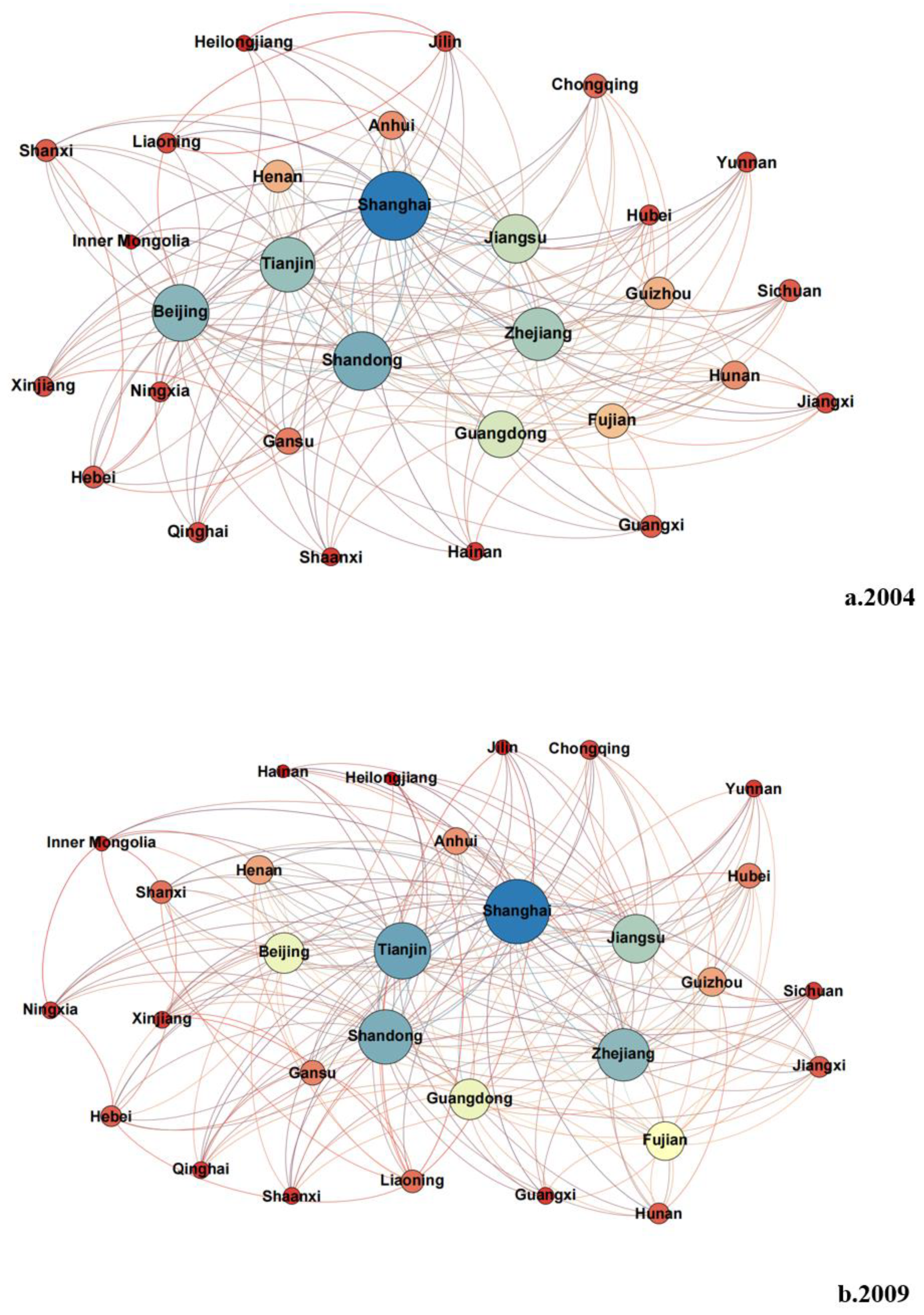
In this paper, we used the modified gravity model to calculate the gravitational matrix of each province between 2004 and 2020 and to visualize the spatial correlation network structure of carbon emission efficiency in the construction industry in China. In addition, Gephi software was chosen to draw the spatial correlation network. The network diagrams are drawn for the years 2004, 2009, 2014, and 2020 with a time interval of 6 years. From Figure 2, we can see that the spatial correlation has broken the limitation of geographic location and has a spatial correlation not only with neighboring provinces but also with non-neighboring provinces [52]. The provinces that are always located at the center of the network include coastal provinces and cities such as Jiangsu, Zhejiang, Shanghai, Guangdong, and Tianjin, which have strong correlations with other provinces due to their high level of low-carbon development in the construction industry, and which enjoy the advantageously geographical location, sound construction, and transportation infrastructure, making it easier for low-carbon exchanges and cooperation in the construction industry. The remaining provinces are at the network’s edge, and the spatial association of carbon emission efficiency in the construction industry shows a “core-edge” network structure.

4.3. Overall Network Structure Characteristics

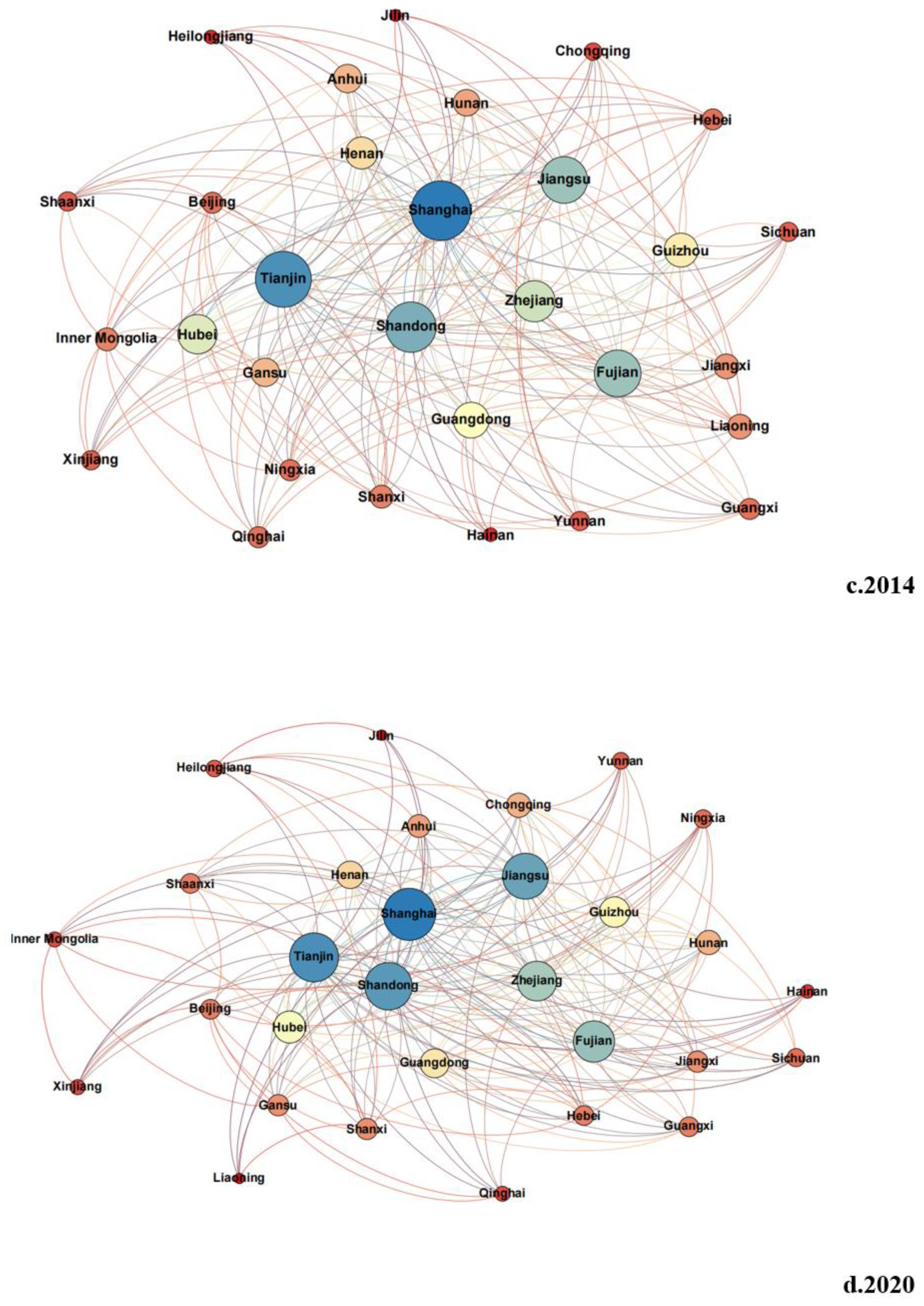
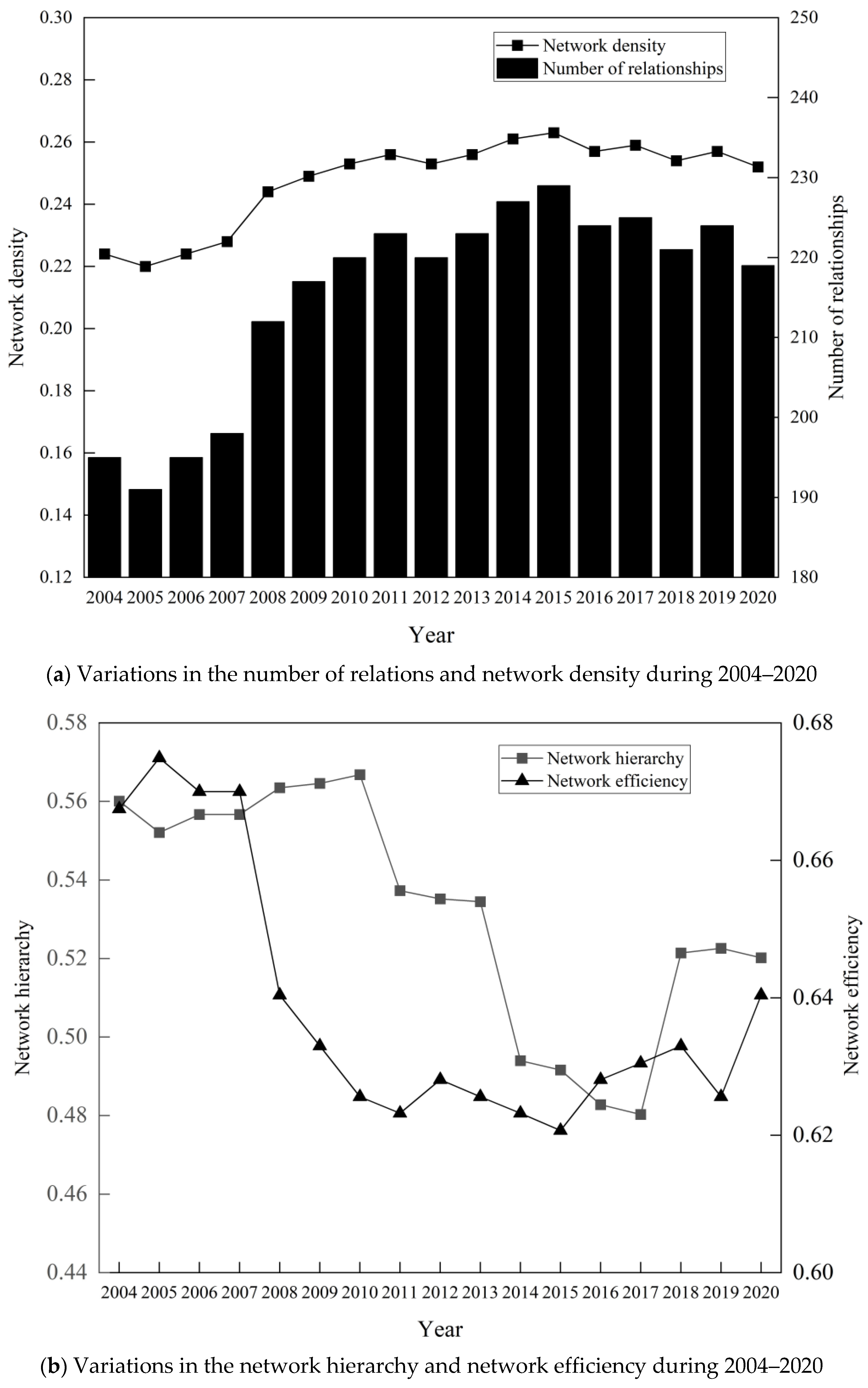
From Figure 3, it can be seen that the overall number of network relationships and network density has steadily increased. The number of network relationships rose from 195 in 2004 to 219 in 2020, of which the maximum value of 229 was reached in 2015. The network density is consistent with the change in the number of network relationships, rising from 0.224 in 2004 to 0.252, of which the maximum value of 0.263 was reached in 2015. According to the above changes, the spatial correlation strength of carbon emission efficiency in China’s construction industry has been strengthened from 2004 to 2020, and the interactions among provinces have been enhanced. However, it is worth noting that there is still a large gap between the existing number of relationships and the maximum possible number of network relationships (870), which indicates that the spatial correlation network needs to be optimized continuously.

The spatial network connectedness remained one during the study period, indicating that the spatial correlation network structure has good connectivity and robustness, and all provinces are in the spatial correlation network. No provinces are out of the network and a significant spillover effect is observed in the network space [53]. The network efficiency decreased from 0.668 in 2004 to 0.640 in 2020, where it reached the minimum value of 0.621 in 2015. This indicates that the number of connections in the spatial network gradually increases with the development of the construction industry, the spatial association among provinces becomes stronger [46], and the spatial network gradually becomes stable. The network ranking degree decreased from 0.560 in 2004 to 0.480 in 2017, then increased to 0.520 in 2020, which indicates that the strict hierarchical structure within the carbon emission efficiency of the construction industry gradually disintegrated, and the interconnection and influence among provinces were strengthened. However, the hierarchy of the carbon emission efficiency network in the construction industry was still high as of 2020, and there is still a specific hierarchical gradient in the spatial correlation network. Thus, the network structure needs to be further optimized [53]. From the above, it can be seen that network density and network efficiency showed high and low inflection points, respectively, in 2015. This may be due to China’s strategy to promote the development of the central region and the western region during the 11th and 12th Five-Year Plans. In addition, in response to the international financial crisis in 2008, the Chinese government launched the “four trillion yuan” stimulus plan and invested much money in infrastructure development [7]. These policies have promoted the balanced development of regional economies and effectively improved energy saving and emission reduction technologies in less developed regions. Therefore, the spatial correlation network exhibits specific cyclical characteristics.

4.4. Individual Network Characteristics

To better compare the evolution of individual networks, the data from 2004 and 2020 is selected to measure in-degree, out-degree, degree centrality, closeness centrality, and betweenness centrality (

Table 3. Centrality analysis of spatial correlation network of carbon emission efficiency of China’s construction industry.

Province	Out-Degree		In-Degree		Degree Centrality		Closeness Centrality		Betweenness Centrality
	2004	2020	2004	2020	2004	2020	2004	2020	2004	2020
Beijing	5	3	21	8	72.414	27.586	76.316	58.000	0.704	0.318
Tianjin	5	5	20	25	72.414	86.207	76.316	87.879	14.783	7.221
Hebei	3	3	6	8	24.138	27.586	56.863	58.000	0.480	0.249
Shanxi	6	6	3	6	20.690	31.034	55.769	59.184	0.846	1.099
Inner Mongolia	4	5	1	3	13.793	27.586	53.704	58.000	0.510	0.193
Liaoning	6	5	2	0	24.138	17.241	56.863	54.717	0.022	0.000
Jilin	6	4	2	1	24.138	17.241	56.863	54.717	0.049	0.015
Heilong jiang	6	9	0	0	20.690	31.034	55.769	59.184	0.849	0.000
Shanghai	5	6	27	26	93.103	89.655	93.548	90.625	11.507	4.678
Jiangsu	2	4	20	24	68.966	82.759	76.316	85.294	8.795	2.915
Zhejiang	5	6	19	18	65.517	65.517	74.359	74.359	4.131	2.743
Anhui	4	6	8	7	27.586	27.586	58.000	58.000	0.286	1.986
Fujian	7	8	8	17	41.379	62.069	63.043	72.500	4.131	9.838
Jiangxi	5	7	3	5	17.241	24.138	52.727	56.863	0.131	2.528
Shandong	7	7	20	22	72.414	79.310	78.378	82.857	8.264	5.633
Henan	6	7	8	9	31.034	31.034	59.184	59.184	0.555	9.315
Hubei	7	11	1	8	27.586	51.724	58.000	67.442	1.234	5.788
Hunan	8	9	4	5	31.034	31.034	59.184	59.184	0.156	1.394
Guang dong	7	9	14	8	58.621	41.379	70.732	63.043	0.732	1.949
Guangxi	7	8	2	3	24.138	31.034	56.863	59.184	0.211	0.464
Hainan	7	7	0	0	24.138	24.138	56.863	56.863	0.131	0.000
Chong qing	9	10	1	4	31.034	37.931	59.184	61.702	0.386	0.945
Sichuan	9	8	0	2	31.034	27.586	59.184	58.000	0.106	0.000
Guizhou	11	11	3	7	41.379	41.379	63.043	63.043	0.783	7.084
Yunnan	8	9	0	0	27.586	31.034	58.000	59.184	0.211	0.000
Shaanxi	7	9	0	2	24.138	31.034	56.863	59.184	0.527	0.671
Gansu	9	11	2	1	37.931	41.379	61.702	63.043	1.636	0.462
Qinghai	8	8	0	0	27.586	27.586	58.000	58.000	0.318	0.000
Ningxia	8	10	0	0	27.586	34.483	58.000	60.417	1.038	0.000
Xinjiang	8	8	0	0	27.586	27.586	58.000	58.000	0.529	0.000
Average	6.5	7.3	6.5	7.3	37.701	40.230	62.588	63.855	2.135	2.250

), which reveal the centrality characteristics of associated individuals in spatial correlation networks [54].

As shown in Table 3, the largest difference between the in-degree and out-degree from 2004 to 2020 was in Beijing, with a difference of 15. This indicates that Beijing’s position in the correlation network is gradually marginalized. There are 10 provinces featuring the in-degree being greater than the out-degree, namely, Jiangsu, Zhejiang, Shanghai, Shandong, Tianjin, Beijing, Hebei, Fujian, and Henan, indicating that these provinces are vulnerable to the carbon emission efficiency of the construction industry in other provinces. The construction industry development level of these provinces is high, which can effectively attract construction talents, capital, low-carbon technology, and other resource factors from all over the world and effectively transform the resource factors to promote the construction industry’s carbon emission efficiency. This makes the network structure show spatial polarization.

(1) Degree centrality. The mean value of the degree centrality of the spatial correlation network of carbon emission efficiency in the construction industry increased from 37.701 in 2004 to 40.230 in 2020. The point degree centrality of nine provinces, namely, Jiangsu, Zhejiang, Shanghai, Guangdong, Tianjin, Shandong, Fujian, Guizhou, and Gansu, is always higher than the mean value, indicating that these provinces have more connections with other provinces in the spatial correlation network and are in the center of the spatial correlation network of carbon emission efficiency in the construction industry. This is because these provinces are mainly located in most of the economically developed coastal areas in the East and the core areas in the central and western parts of China, with relatively sound transportation infrastructures and ideal geographic locations so that they can communicate more smoothly with other provinces on low-carbon development. At the same time, the low-carbon technologies in the construction industry in these provinces are more advanced, which can quickly generate the “siphon phenomenon” and low-carbon technology spillover effects. The provinces with a low degree of centrality are located in the northeastern and western regions led by Liaoning, Jilin, Xinjiang, Qinghai, etc. These provinces are remote, with a weak economic base, less convenient transportation, and less connected with other provinces. Therefore, they are in a marginal position in the construction industry spatial association network.

(2) Closeness centrality. The mean value of the closeness centrality of the spatial correlation network of carbon emission efficiency in the construction industry increased from 62.588 in 2004 to 63.855 in 2020. The maximum value decreased from 93.548 in 2004 to 90.625 in 2020. The minimum value increased from 52.727 in 2004 to 54.717. The values of the above three variables do not change much, which indicates that the spatial association network is generally in a relatively balanced state. The closeness centrality of seven provinces, namely, Jiangsu, Zhejiang, Shanghai, Tianjin, Shandong, Fujian, and Hubei, is higher than the average. These provinces enjoy geographical advantages and play the role of core actors in the spatial correlation network, leading to more spatial connections with other provinces [49]. The closeness centrality of provinces such as Liaoning and Jilin is lower. Due to economic development and geographical constraints, it is hard for these provinces to access advanced low-carbon technologies and development resources from other provinces and suffer from less significant spatial spillover from other provinces. Therefore, they play the role of marginal actors in the network and it is necessary for these provinces to gain more links with other provinces.

(3) Betweenness centrality. The mean value of betweenness centrality of the spatial correlation network of carbon emission efficiency in the construction industry increased from 2.135 in 2004 to 2.250 in 2020, and the number of provinces above the mean value increased from 6 to 10. This indicates that the dominant role of the central node of the network shows an upward tendency. In 2020, the betweenness centrality of 10 provinces, namely, Jiangsu, Zhejiang, Shanghai, Tianjin, Shandong, Fujian, Jiangxi, Henan, Hubei, and Guizhou, was higher than the average value, accounting for 85.56% of the national betweenness centrality. It shows that these provinces have substantial control over the resources such as talents, information, capital, and technology in the spatial correlation network. At the same time, they have a more vital ability to facilitate the establishment of links with other provinces and are in the position of network hubs in the spatial correlation network. This makes them play the role of “intermediaries” and “bridges” in the network. In particular, Hubei, Henan, Guizhou, and Fujian have become important links and fulcrums for promoting the flow of carbon emission efficiency factors and resources from the eastern coastal region to the southwest and northwest regions due to their special geographical location. They serve as a link between the east and the west, as well as the north and the south [54]. While the remaining provinces only accounted for 14.44% of the national intermediary center, most of these provinces were remote and had weak economic bases and outdated technology. Furthermore, they have weak control over resource factors and were in a marginal position in the network dominated by other provinces. Therefore, we need to optimize the structure of the spatial correlation network of carbon emission efficiency in the construction industry to improve the imbalance between the former and the latter, which has a massive gap in the control of resource factors.

4.5. Network Clustering Characteristics

To ensure that the research results are more in line with the current situation [55]. This paper uses the CONCOR module in Ucinet (maximum partition density set to 2 and convergence criterion set to 0.2) to perform a block model clustering analysis on the spatial correlation network of carbon emission efficiency of the construction industry in 30 Chinese provinces in 2020, and the analysis results divide the 30 Chinese provinces into four segments [56]. As seen from

Table 4. Division of plates.

Plate	Province
First plate (I)	Anhui, Henan, Shanxi, Heilongjiang, Liaoning, Xinjiang, Gansu, Qinghai, Ningxia, Jilin
Second plate (II)	Guangdong, Chongqing, Hunan, Shaanxi, Guangxi, Sichuan, Hubei, Jiangxi, Hainan, Gansu, Yunnan
Third plate (III)	Beijing, Inner Mongolia, Hebei
Fourth plate (IV)	Jiangsu, Zhejiang, Shanghai, Shandong, Tianjin, Fujian

, the number of intra-slab relationships in the spatial correlation network total 50, accounting for 22.83% of the total network relationships in 2020. The number of extra-slab relationships totals 169, accounting for 77.17% of the total network relationships in 2020, showing a significant spatial clustering effect and spatial spillover in the carbon emission efficiency of the construction industry in each province [57]. The distribution of provinces in the four plates is shown in Table 4.

In the first plate, the number of relationships within the plate is 6. The number of outgoing and incoming relationships outside the plate is 68 and 18, respectively, with fewer relationships within the plate and more overflow outside the plate. At the same time, the actual proportion of internal relationships within the plate is 8.11%, which is less than the desired proportion of internal relationships of 31.04%. Therefore, the first plate belongs to the “net outflow plate”. In the second plate, the number of intra-block relationships is 30. The number of outgoing and incoming relationships outside the block are 68 and 14, respectively, with the close spatial association of both internal and external network members; meanwhile, the actual internal relationship ratio is 30.61%, which is smaller than the desired internal relationship ratio of 34.48%. Therefore, the second plate belongs to the “agent plate”, which acts as a communication link among elements in the whole spatial correlation network [57]. Most of the provinces in the second plate are geographically located at the junction of the three regions. It is evitable that the second plate is the only path to transmit exchanges of low-carbon technologies and natural resources between the east and the west. At the same time, provinces in the second plate are internally adjacent to each other and communicate very closely, which makes them act as a link. The number of intra-plate relations in the third plate is 3, while the number of outgoing and incoming relations outside the plate are 8 and 15, respectively, with a small difference between the number of outgoing and incoming relations. In addition, the ratio of expected internal relations is 6.90%, which is smaller than the actual ratio of internal relations of 27.27%. Therefore, the third plate is a “bidirectional spillover plate”. In the fourth plate, the number of in-panel relationships is 11, while the number of out-plate relationships and in-plate relationships is 25 and 122, respectively. The number of in-plate relationships is much larger than out-plate relationships. Moreover, the actual internal relationship ratio is 30.56%, which is larger than the actual internal relationship ratio of 17.24%. Therefore, the fourth plate belongs to the “net inflow plate”. The reason for this is that the provinces in the fourth sector are located in the center of the spatial correlation network of the construction industry and are vulnerable to the spillover effects of other provinces. They are also located in the eastern coastal regions, with superior geographical locations and good transportation facilities. However, insufficient natural resources limit development. As a result, they rely on the resources from other provinces to promote their construction industry’s low-carbon development, which shapes their position of “net inflow plate”.

From the above, we can see that the four significant segments play different roles in forming the spatial correlation network of carbon emission efficiency in China’s construction industry. In this paper, the network density matrix of the four major sectors is converted into a like matrix (the value of 1 for the network density matrix greater than 0.252 and 0 otherwise), which is used to explore further the spatial network relationship among the four major sectors. As shown in

Table 5. Spillover relationship and its image matrix between spatially related sectors of China’s construction industry carbon emission efficiency.

Plate		I	II	III	IV
Outflow relation	Inside the plate	6	30	3	11
	Outside the plate	68	68	8	25
Inflow relation	Inside the plate	6	30	3	11
	Outside the plate	18	14	15	122
Expected internal relationship ratio %		31.03%	34.48%	6.90%	17.24%
Actual internal relationship ratio %		8.11%	30.61%	27.27%	30.56%
Image matrix	I	0	0	1	1
	II	0	1	0	1
	III	0	0	1	1
	Ⅳ	0	0	0	1

, the first, second, and third plates all produce spatial spillover to the fourth plate, and there is a connection within the fourth plate, which indicates that the fourth plate is in the center of the network, and the other plates provide the required resource to it. In addition, there are also internal linkages within the second and third sectors, and the first sector also generates spatial spillover to the third sector.

4.6. Spatial Correlation Network Structure Formation Mechanism

4.6.1. QAP Correlation Analysis

To investigate the formation mechanism of the spatial correlation network of carbon emission efficiency in the construction industry. This paper adopts the QAP model to conduct regression analysis on the influencing factors. Before the QAP regression is conducted, QAP correlation analysis is used to measure the correlation between the spatial correlation network of carbon emission efficiency in the construction industry and each influencing factor to explain whether it is suitable for applying QAP regression analysis. Therefore, this paper set the number of random permutations to 5000, and the QAP correlation analysis results are obtained using UCINET 6. As seen from

Table 6. QAP correlation analysis and regression analysis.

Variable	Correlation Coefficient	p Value	Regression Coefficient	p Value
C	0.195	0.000	0.339	0.000
P	0.390	0.000	0.341	0.000
U	0.262	0.000	0.084	0.033
T	0.049	0.035	0.024	0.536
L	−0.049	0.073	−0.024	0.787
A	0.039	0.032	0.053	0.041
I	0.037	0.253	—	—
R2	—	—	0.231
Adjustment R2	—	—	0.226

, the correlation coefficients of geographical proximity, regional economic level gap, and urbanization level gap are positive at a 1% significance level, indicating that they are significantly and positively correlated with the spatial correlation network of carbon emission efficiency in the construction industry. At the 5% significance level, the correlation coefficients of the energy efficiency technology gap and the industrial agglomeration gap are positive. Revealing that they are significantly and positively correlated with the spatial correlation network of carbon emission efficiency in the construction industry. At the 10% significance level, the labor productivity gap negatively influences the formation of the spatial correlation network, and the gap in the industrial development level is not correlated with the formation of a spatial association network. Therefore, this factor is excluded from the paper.

Table 7. Correlation Matrix between Variables.

Variable	A	U	P	T	C	L
A	1 ***
U	0.041	1 ***
P	0.060	0.554 ***	1 ***
T	0.139 **	0.153 **	0.243 ***	1 ***
C	−0.154 ***	−0.158 ***	−0.159 ***	−0.064 **	1 ***
L	0.139 **	0.153 **	0.243 ***	1 ***	−0.064 *	1 ***

Note: *** indicates significant at 1% level, ** indicates significant at 5% level, and * indicates significant at 10% level.

shows the correlations among the variables, and it can be seen from Table 7 that there is a multicollinearity problem among the variables. To address this problem that exists in the explanatory variables, this paper uses QAP for regression analysis.

4.6.2. QAP Regression Analysis

As above, the number of random permutations is set to 5000 to study the formation mechanism of the spatial association network in this paper. The QAP regression results are shown in Table 6. The adjusted R² is 0.226, which indicates that geographic proximity, regional economic level gap, urbanization level gap, energy saving technology level gap, and industrial agglomeration gap can explain 22.6% of the spatial correlation effect. From Table 6, geographical proximity is significant at a 1% level, of which the regression coefficient is positive, indicating that geographical proximity has a positive effect on the formation of the spatial correlation network. This is because commercial linkages and resource transportation are more common in geographically adjacent provinces, thus strengthening the spatial links [7]. Regional differences in economic levels are significant at the 1% level, and their regression coefficients are positive, revealing that more significant regional differences are able to strengthen the spatial correlation. This is mainly because the more significant the “potential energy difference” between regions, the more significant the “siphon effect” and “trickle-down effect” of factors under the action of market mechanism [54], representing that, on the one hand, provinces with high regional economic levels tend to attract capital inflows from other provinces so that provinces with higher economic levels have enough capital to adopt better energy-saving technologies [40], while, on the other hand, provinces with weak economic development and abundant resources provide their resources for these high-tech provinces for further processing, both of which contribute to a closer spatial correlation of carbon emission efficiency in the construction industry. The urbanization level gap is significant at the 5% level, of which the regression coefficient is positive, indicating that the larger the urbanization level gap is, the stronger the spatial correlation, similar to the regional economic level gap. The industrial agglomeration gap is significant at the 5% level, and its regression coefficient is small and negative, which means that regions with similar types of industrial agglomeration are more likely to generate spatial spillover because they have the same development model. In addition, their low-carbon exchanges are not hindered, making them more closely linked spatially. Although the regression coefficients of the energy-saving technology level and labor productivity gap are positive, they do not significantly affect forming of a spatial correlation network of carbon emission efficiency in the construction industry.

5. Discussion

This paper provides a new perspective for the spatial analysis of carbon emission efficiency in China’s construction industry. Firstly, this paper adopts a global non-expected output super-efficiency EBM model to measure the carbon emission efficiency of the construction industry in 30 Chinese provinces. The global EBM model achieves comparability of efficiency across periods while solving the inherent problems of radial and non-radial models, namely, the radial DEA model ignores the influence of non-radial slack variables, while the non-radial SBM model tends to neglect the original between the target and actual values, resulting in an underestimation of the actual performance when evaluating invalid DMUs [35]. Secondly, this paper constructs a spatial correlation matrix by using the modified gravity model, which overcomes the time lag of the traditional VAR model and can analyze the evolution characteristics of the network structure through cross-sectional data. The modified gravity model considers the geographic proximity and relevant factors (population size and regional economic level) that affect the emission efficiency of the construction industry, which can better reflect spatial characteristics [7]. This model has been widely used in constructing spatial association matrices [36,43,55]. Again, this paper analyzes the overall network characteristics, individual network characteristics, and spatial aggregation characteristics and finds that the carbon emission efficiency of China’s construction industry has broken the traditional geospatial proximity restriction, manifesting a complex, multi-threaded spatial correlation [53]. The spatial correlation network shows a “core-edge” network structure, and the provinces at the center of the network belong to the “net inflow plate”. Finally, the QAP method can overcome the problems of multicollinearity and autocorrelation. Therefore, this paper applies this method to the correlation and regression analysis of the factors influencing spatial correlation. It is found that geographical proximity is the most critical factor in the formation of the spatial correlation network [46,58,59,60], and the differences in regional economic levels and urbanization levels also largely contribute to the formation of the spatial correlation network [56]. The similarity of regional industrial agglomerations contributes to the formation of the spatial correlation network as well.

Given the above research, there are still some limitations in this research. First, due to the availability of data, this paper only studies the spatial correlation network at the provincial level, lacking more in-depth research. In the future, it is advisable for scholars to dig deep into the data and explore the spatial correlation network at the municipal level. Secondly, the adjusted R² of QAP regression is only 0.226, which shows that the selection of influencing factors is one-sided, and more factors need to be added in future research to further explore the formation mechanism of the spatial correlation network. Finally, our discussion of policy recommendations is limited to the macro level. In the future, we will carry out further detailed research on the cost of policy recommendations.

6. Conclusions and Policy Recommendations

6.1. Conclusions

This paper first measured the carbon emission efficiency of China’s construction industry in 30 provinces from 2004 to 2020 via the global super-efficiency EBM model, then revealed the evolution characteristics of the spatial association network of the carbon emission efficiency of China’s construction industry by the modified gravity model and social network analysis. Finally, the QAP model was used to investigate the formation mechanism of the spatial association network. The main findings of this paper are as follows:

(1) From 2004 to 2020, the carbon emission efficiency of China’s construction industry increased from 0.171 in 2004 to 0.538 in 2020, with an overall steady increase. The carbon emission efficiency of the construction industry showed a spatial distribution pattern of “high in the east and low in the west”, indicating the differences between provinces were gradually increasing.

(2) During the study period, the carbon emission efficiency of China’s construction industry has broken the traditional geospatial proximity restriction, presenting a complex, multi-threaded spatial correlation, with the spatial correlation network showing a “core-edge” network structure. From the overall network characteristics, the network density and efficiency showed an upward and downward trend, respectively, during the study period, and the network connectedness was always 1. From the perspective of individual network characteristics, the eastern regions of Jiangsu, Zhejiang, Shanghai, Tianjin, and Shandong have been at the center of the network, playing the role of “core actor” in the spatial correlation network and playing essential roles in “intermediary” and “bridge” as well. From the perspective of network aggregation characteristics, the spatial correlation network can be divided into “bidirectional spillover plate”, “net inflow plate”, “net outflow plate”, and “agent plate”. Most of the provinces located in the center of the network belong to the “net inflow plate”, and most of the provinces located at the junction of the three regions belong to the “agent plate”, which plays the role of a link. (3) The results of QAP correlation and regression analysis show that geographic proximity, regional economic level differences, and urbanization differences have a significant positive impact on the formation of the spatial correlation network. The industrial agglomeration gap has a significant negative impact on the formation of the spatial correlation network. However, the regression coefficients of differences in energy-saving technology levels and differences in labor productivity are positive but not significant, and their impact mechanisms still need to be further improved and strengthened.

6.2. Policy Recommendations

To achieve the goal of “carbon peak, carbon neutrality” as soon as possible, the following suggestions for cross-regional collaborative carbon reduction in the construction industry are proposed based on the results of the study:

Firstly, the government should establish a cross-regional collaborative carbon emission reduction mechanism for carbon emission efficiency in the construction industry, pay attention to the spatial correlation effect of carbon emission efficiency, strengthen the low-carbon development exchange among geographically adjacent provinces, consider the issues related to cross-regional collaborative management of carbon emission in the construction industry from the perspective of the overall network structure [47], and coordinate the actions of all parties under the overall layout to form a 1 + 1 > 2 emission reduction effect. Secondly, the government should optimize the spatial correlation network structure of carbon emission efficiency in the construction industry, focus on breaking the spatial network hierarchy, encourage Jiangsu, Zhejiang, Shanghai, Tianjin, Shandong, and other eastern regions to play the leading role in the spatial correlation network [55], and improve the spatial spillover effect of low-carbon technologies in the central provinces of the network to promote the low-carbon development of the construction industry in other provinces. Provinces at the edge of the network should take advantage of the abundant resources, strengthen the economic exchanges with the central provinces of the network, and strive to become the central position of the network. Thirdly, the characteristics of the four plates in the spatial correlation network of carbon emission efficiency in the construction industry should be fully considered, and regionally differentiated policies for carbon emission reduction in construction should be formulated. For provinces in the “bidirectional spillover plate” and the “net outflow plate”, the government should promote low-carbon technology innovation and green building materials. In addition, the government should learn from foreign advanced building energy efficiency and low-carbon technologies and use industrial transfer methods to solve the problem of high carbon emissions while taking on more carbon emission reduction tasks. For provinces in the “net inflow plate, they should introduce advanced low-carbon technologies to improve energy efficiency and make full use of resources to develop wind power, photovoltaic, and other clean energy technologies. Provinces in the “agent plate” should take advantage of their geographical location to connect the eastern and western regions, continue to strengthen the role of regional exchange links, build bridges between the eastern and western regions for carbon emission reduction in the construction industry, and further promote the flow of low-carbon technologies. In addition, the government should strengthen the mutual communication among the four major sectors and implement a cross-sector collaborative carbon emission reduction mechanism. Fourth, the government should consider the impact of regional development, urbanization, and industrial agglomeration gap on forming a spatial correlation network. On the one hand, the government should balance the advantages and disadvantages of regional development and urbanization disparities and strengthen the spatial linkage between regions while narrowing the gap. On the other hand, the government should establish a similar industrial agglomeration model for each province, and provinces with lower carbon emission efficiency should learn the industrial distribution model of provinces with higher carbon emission efficiency to optimize the industrial structure within the provinces and effectively promote the formation of a spatial correlation network.

References

- Lu, N.; Feng, S.; Liu, Z.; Wang, W.; Lu, H.; Wang, M. The Determinants of Carbon Emissions in the Chinese Construction Industry: A Spatial Analysis. Sustainability 2020, 12, 1428. [Google Scholar] [CrossRef] [Green Version]
- Lu, Y.; Cui, P.; Li, D. Carbon Emissions and Policies in China’s Building and Construction Industry: Evidence from 1994 to 2012. Build. Environ. 2016, 95, 94–103. [Google Scholar] [CrossRef]
- Zhang, P.; Hu, J.; Zhao, K.; Chen, H.; Zhao, S.; Li, W. Dynamics and Decoupling Analysis of Carbon Emissions from Construction Industry in China. Buildings 2022, 12, 257. [Google Scholar] [CrossRef]
- Ma, X.; Wang, C.; Dong, B.; Gu, G.; Chen, R.; Li, Y.; Zou, H.; Zhang, W.; Li, Q. Carbon Emissions from Energy Consumption in China: Its Measurement and Driving Factors. Sci. Total Environ. 2019, 648, 1411–1420. [Google Scholar] [CrossRef] [PubMed]
- Mallapaty, S. How China Could Be Carbon Neutral by Mid-Century. Nature 2020, 586, 482–483. [Google Scholar] [CrossRef]
- Normile, D. China’s Bold Climate Pledge Earns Praise—But Is It Feasible? Science 2020, 370, 17–18. [Google Scholar] [CrossRef]
- Li, S.; Wu, Q.; Zheng, Y.; Sun, Q. Study on the Spatial Association and Influencing Factors of Carbon Emissions from the Chinese Construction Industry. Sustainability 2021, 13, 1728. [Google Scholar] [CrossRef]
- Wang, M.; Feng, C. Exploring the Driving Forces of Energy-Related CO2 Emissions in China’s Construction Industry by Utilizing Production-Theoretical Decomposition Analysis. J. Clean. Prod. 2018, 202, 710–719. [Google Scholar] [CrossRef]
- Li, R.; Jiang, R. Moving Low-Carbon Construction Industry in Jiangsu Province: Evidence from Decomposition and Decoupling Models. Sustainability 2017, 9, 1013. [Google Scholar] [CrossRef] [Green Version]
- Du, Q.; Wu, M.; Wang, N.; Bai, L. Spatiotemporal Characteristics and Influencing Factors of China’s Construction Industry Carbon Intensity. Pol. J. Environ. Stud. 2017, 26, 2507–2521. [Google Scholar] [CrossRef] [Green Version]
- Li, Y.; Zhang, S. Spatio-Temporal Evolution of Urban Carbon Emission Intensity and Spatio-Temporal Heterogeneity of Influencing Factors in China. China Environ. Sci. 2023. [Google Scholar] [CrossRef]
- Peng, Z.; Wu, Q.; Wang, D.; Li, M. Temporal-Spatial Pattern and Influencing Factors of China’s Province-Level Transport Sector Carbon Emissions Efficiency. Pol. J. Environ. Stud. 2020, 29, 233–247. [Google Scholar] [CrossRef] [PubMed]
- Gao, P.; Yue, S.; Chen, H. Carbon Emission Efficiency of China’s Industry Sectors: From the Perspective of Embodied Carbon Emissions. J. Clean. Prod. 2021, 283, 124655. [Google Scholar] [CrossRef]
- Wang, M.; Feng, C. The Consequences of Industrial Restructuring, Regional Balanced Development, and Market-Oriented Reform for China’s Carbon Dioxide Emissions: A Multi-Tier Meta-Frontier DEA-Based Decomposition Analysis. Technol. Forecast. Soc. Chang. 2021, 164, 120507. [Google Scholar] [CrossRef]
- Zhu, Q.; Li, X.; Li, F.; Zhou, D. The Potential for Energy Saving and Carbon Emission Reduction in China’s Regional Industrial Sectors. Sci. Total Environ. 2020, 716, 135009. [Google Scholar] [CrossRef]
- Ding, L.; Yang, Y.; Wang, W.; Calin, A.C. Regional Carbon Emission Efficiency and Its Dynamic Evolution in China: A Novel Cross Efficiency-Malmquist Productivity Index. J. Clean. Prod. 2019, 241, 118260. [Google Scholar] [CrossRef]
- Wang, Y.; Duan, F.; Ma, X.; He, L. Carbon Emissions Efficiency in China: Key Facts from Regional and Industrial Sector. J. Clean. Prod. 2019, 206, 850–869. [Google Scholar] [CrossRef]
- Wang, X.; Shen, Y.; Su, C. Spatial—Temporal Evolution and Driving Factors of Carbon Emission Efficiency of Cities in the Yellow River Basin. Energy Rep. 2023, 9, 1065–1070. [Google Scholar] [CrossRef]
- Wang, R.; Feng, Y. Research on China’s Agricultural Carbon Emission Efficiency Evaluation and Regional Differentiation Based on DEA and Theil Models. Int. J. Environ. Sci. Technol. 2021, 18, 1453–1464. [Google Scholar] [CrossRef]
- Liu, F.; Tang, L.; Liao, K.; Ruan, L.; Liu, P. Spatial Distribution and Regional Difference of Carbon Emissions Efficiency of Industrial Energy in China. Sci. Rep. 2021, 11, 19419. [Google Scholar] [CrossRef]
- Li, S.; Cheng, Z.; Tong, Y.; He, B. The Interaction Mechanism of Tourism Carbon Emission Efficiency and Tourism Economy High-Quality Development in the Yellow River Basin. Energies 2022, 15, 6975. [Google Scholar] [CrossRef]
- Xu, H.; Li, Y.; Zheng, Y.; Xu, X. Analysis of Spatial Associations in the Energy–Carbon Emission Efficiency of the Transportation Industry and Its Influencing Factors: Evidence from China. Environ. Impact Assess. Rev. 2022, 97, 106905. [Google Scholar] [CrossRef]
- Song, H.; Gu, L.; Li, Y.; Zhang, X.; Song, Y. Research on Carbon Emission Efficiency Space Relations and Network Structure of the Yellow River Basin City Cluster. Int. J. Environ. Res. Public Health 2022, 19, 12235. [Google Scholar] [CrossRef]
- Tang, Y.; Yang, Z.; Yao, J.; Li, X.; Chen, X. Carbon Emission Efficiency and Spatially Linked Network Structure of China’s Logistics Industry. Front. Environ. Sci. 2022, 10, 2057. [Google Scholar] [CrossRef]
- Zhou, W.; Yu, W. Regional Variation in the Carbon Dioxide Emission Efficiency of Construction Industry in China: Based on the Three-Stage DEA Model. Discret. Dyn. Nat. Soc. 2021, 2021, 4021947. [Google Scholar] [CrossRef]
- Zhang, G.; Jia, N. Measurement and Spatial Correlation Characteristics of Carbon Emission Efficiency in China’s Construction Industry. Sci. Technol. Manag. Res. 2019, 21, 236–242. [Google Scholar] [CrossRef]
- Yang, Z.; Fang, H.; Xue, X. Sustainable Efficiency and CO2 Reduction Potential of China’s Construction Industry: Application of a Three-Stage Virtual Frontier SBM-DEA Model. J. Asian Archit. Build. Eng. 2022, 21, 604–617. [Google Scholar] [CrossRef]
- Li, W.; Wang, W.; Gao, H.; Zhu, B.; Gong, W.; Liu, Y.; Qin, Y. Evaluation of Regional Metafrontier Total Factor Carbon Emission Performance in China’s Construction Industry: Analysis Based on Modified Non-Radial Directional Distance Function. J. Clean. Prod. 2020, 256, 120425. [Google Scholar] [CrossRef]
- Cheng, M.; Lu, Y.; Zhu, H.; Xiao, J. Measuring CO2 Emissions Performance of China’s Construction Industry: A Global Malmquist Index Analysis. Environ. Impact Assess. Rev. 2022, 92, 106673. [Google Scholar] [CrossRef]
- Zhou, Y.; Liu, W.; Lv, X.; Chen, X.; Shen, M. Investigating Interior Driving Factors and Cross-Industrial Linkages of Carbon Emission Efficiency in China’s Construction Industry: Based on Super-SBM DEA and GVAR Model. J. Clean. Prod. 2019, 241, 118322. [Google Scholar] [CrossRef]
- Zhou, Y.; Lv, S.; Wang, J.; Tong, J.; Fang, Z. The Impact of Green Taxes on the Carbon Emission Efficiency of China’s Construction Industry. Sustainability 2022, 14, 5402. [Google Scholar] [CrossRef]
- Hui, M.; Su, Y. Spatial characteristics of carbon emission efficiency in China construction industry and its influencing factors. Environ. Eng. 2018, 12, 182–187. [Google Scholar] [CrossRef]
- Du, Q.; Deng, Y.; Zhou, J.; Wu, J.; Pang, Q. Spatial Spillover Effect of Carbon Emission Efficiency in the Construction Industry of China. Environ. Sci. Pollut. Res. 2022, 29, 2466–2479. [Google Scholar] [CrossRef] [PubMed]
- Huo, T.; Cao, R.; Xia, N.; Hu, X.; Cai, W.; Liu, B. Spatial Correlation Network Structure of China’s Building Carbon Emissions and Its Driving Factors: A Social Network Analysis Method. J. Environ. Manag. 2022, 320, 115808. [Google Scholar] [CrossRef]
- Yang, Q.; Si, X.; Wang, J. The Measurement and Its Distribution Dynamic Evolution of Grain Production Efficiency in China under the Goal of Reducing Pollution Emissions and Increasing Carbon Sink. J. Nat. Resour. 2022, 37, 600. [Google Scholar] [CrossRef]
- Ma, F.; Wang, Y.; Yuen, K.F.; Wang, W.; Li, X.; Liang, Y. The Evolution of the Spatial Association Effect of Carbon Emissions in Transportation: A Social Network Perspective. Int. J. Environ. Res. Public Health 2019, 16, 2154. [Google Scholar] [CrossRef] [Green Version]
- Pastor, J.T.; Lovell, C.A.K. A Global Malmquist Productivity Index. Econ. Lett. 2005, 88, 266–271. [Google Scholar] [CrossRef]
- Avkiran, N.K.; Tone, K.; Tsutsui, M. Bridging Radial and Non-Radial Measures of Efficiency in DEA. Ann. Oper. Res. 2008, 164, 127–138. [Google Scholar] [CrossRef]
- Tone, K.; Tsutsui, M. An Epsilon-Based Measure of Efficiency in DEA—A Third Pole of Technical Efficiency. Eur. J. Oper. Res. 2010, 207, 1554–1563. [Google Scholar] [CrossRef]
- Yu, Z.; Chen, L.; Tong, H.; Chen, L.; Zhang, T.; Li, L.; Yuan, L.; Xiao, J.; Wu, R.; Bai, L.; et al. Spatial Correlations of Land-Use Carbon Emissions in the Yangtze River Delta Region: A Perspective from Social Network Analysis. Ecol. Indic. 2022, 142, 109147. [Google Scholar] [CrossRef]
- Chen, H.; Zhu, S.; Sun, J.; Zhong, K.; Shen, M.; Wang, X. A Study of the Spatial Structure and Regional Interaction of Agricultural Green Total Factor Productivity in China Based on SNA and VAR Methods. Sustainability 2022, 14, 7508. [Google Scholar] [CrossRef]
- Lao, X.; Zhang, X.; Shen, T.; Skitmore, M. Comparing China’s City Transportation and Economic Networks. Cities 2016, 53, 43–50. [Google Scholar] [CrossRef] [Green Version]
- Song, J.; Feng, Q.; Wang, X.; Fu, H.; Jiang, W.; Chen, B. Spatial Association and Effect Evaluation of CO2 Emission in the Chengdu-Chongqing Urban Agglomeration: Quantitative Evidence from Social Network Analysis. Sustainability 2019, 11, 1. [Google Scholar] [CrossRef] [Green Version]
- Zhang, Z.; Wang, Z.; Zhang, W.; Liu, Y.; Li, Z.; Huang, L. The Complexity of Urban CO2 Emission Network: An Exploration of the Yangtze River Middle Reaches Megalopolis, China. Complexity 2021, 2021, 6612363. [Google Scholar] [CrossRef]
- Li, X.; Feng, D.; Li, J.; Zhang, Z. Research on the Spatial Network Characteristics and Synergetic Abatement Effect of the Carbon Emissions in Beijing-Tianjin-Hebei Urban Agglomeration. Sustainability 2019, 11, 1444. [Google Scholar] [CrossRef] [Green Version]
- He, Y.; Wei, Z.; Liu, G.; Zhou, P. Spatial Network Analysis of Carbon Emissions from the Electricity Sector in China. J. Clean. Prod. 2020, 262, 121193. [Google Scholar] [CrossRef]
- Rong, T.; Zhang, P.; Zhu, H.; Jiang, L.; Li, Y.; Liu, Z. Spatial Correlation Evolution and Prediction Scenario of Land Use Carbon Emissions in China. Ecol. Inform. 2022, 71, 101802. [Google Scholar] [CrossRef]
- Wang, Z.; Zhou, Y.; Zhao, N.; Wang, T.; Zhang, Z. Spatial Correlation Network and Driving Effect of Carbon Emission Intensity in China’s Construction Industry. Buildings 2022, 12, 201. [Google Scholar] [CrossRef]
- Liu, J.; Song, J.Q. Space network structure and formation mechanism of green innovation efficiency of tourism industry in China. China Popul. Resour. Environ. 2018, 8, 127–137. [Google Scholar] [CrossRef]
- Sun, L.; Qin, L.; Taghizadeh-Hesary, F.; Zhang, J.; Mohsin, M.; Chaudhry, I.S. Analyzing Carbon Emission Transfer Network Structure among Provinces in China: New Evidence from Social Network Analysis. Environ. Sci. Pollut. Res. 2020, 27, 23281–23300. [Google Scholar] [CrossRef]
- Li, T.; Gao, H.; Yu, J. Analysis of the Spatial and Temporal Heterogeneity of Factors Influencing CO2 Emissions in China’s Construction Industry Based on the Geographically and Temporally Weighted Regression Model: Evidence from 30 Provinces in China. Front. Environ. Sci. 2022, 10, 1057387. [Google Scholar] [CrossRef]
- Zhang, T.; Wu, J.S. Spatial Network Structure and Influence Mechanism of Green Development Efficiency of Chinese Cultural Industry. Sci. Geogr. Sin. 2021, 4, 580–587. [Google Scholar] [CrossRef]
- Shao, Q.H.; Wang, Z.F. Spatial network structure of transportation carbon emissions efficiency in China and its influencing factors. China Popul. Resour. Environ. 2021, 19, 32–41. [Google Scholar] [CrossRef]
- Zhao, L.; Cao, N.; Han, Z.; Gao, X. Spatial Correlation Network and Influencing Factors of Green Economic Efficiency in China. Editor. Board Resour. Sci. 2021, 43, 1933–1946. [Google Scholar] [CrossRef]
- Yang, G.; Gong, G.; Gui, Q. Exploring the Spatial Network Structure of Agricultural Water Use Efficiency in China: A Social Network Perspective. Sustainability 2022, 14, 2668. [Google Scholar] [CrossRef]
- Wang, F.; Gao, M.; Liu, J.; Fan, W. The Spatial Network Structure of China’s Regional Carbon Emissions and Its Network Effect. Energies 2018, 11, 2706. [Google Scholar] [CrossRef] [Green Version]
- Shang, J.; Ji, X.; Shi, R.; Zhu, M. Structure and Driving Factors of Spatial Correlation Network of Agricultural Carbon Emission Efficiency in China. Chin. J. Eco-Agric. 2022, 30, 543–557. [Google Scholar] [CrossRef]
- Qu, H.; Yin, Y.; Li, J.; Xing, W.; Wang, W.; Zhou, C.; Hang, Y. Spatio-Temporal Evolution of the Agricultural Eco-Efficiency Network and Its Multidimensional Proximity Analysis in China. Chin. Geogr. Sci. 2022, 32, 724–744. [Google Scholar] [CrossRef]
- Qin, H.; Huang, Q.; Zhang, Z.; Lu, Y.; Li, M.; Xu, L.; Chen, Z. Carbon Dioxide Emission Driving Factors Analysis and Policy Implications of Chinese Cities: Combining Geographically Weighted Regression with Two-Step Cluster. Sci. Total Environ. 2019, 684, 413–424. [Google Scholar] [CrossRef]
- Yang, C.; Liu, S. Spatial Correlation Analysis of Low-Carbon Innovation: A Case Study of Manufacturing Patents in China. J. Clean. Prod. 2020, 273, 122893. [Google Scholar] [CrossRef]
Figure 1.
Carbon emission efficiency of the construction industry in China across three regions.
Figure 2.
Spatial Network Structure of Carbon Emission Efficiency of China’s Construction Industry in 2004, 2009, 2014, and 2020.