
Artificial Intelligence for the Detection of Asbestos Cement Roofing: An Investigation of Multi-Spectral Satellite Imagery and High-Resolution Aerial Imagery


Abstract
:1. Introduction
1.1. Asbestos in Australia
1.2. Asbestos Identification vs. ACM Detection
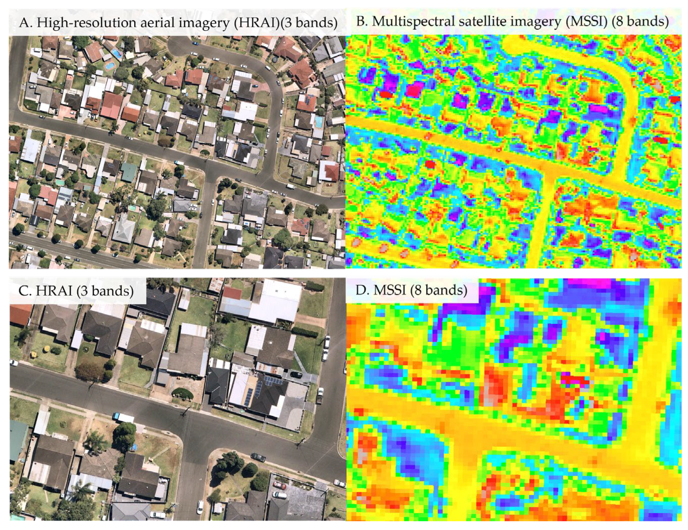
1.3. Remote Sensing Imagery
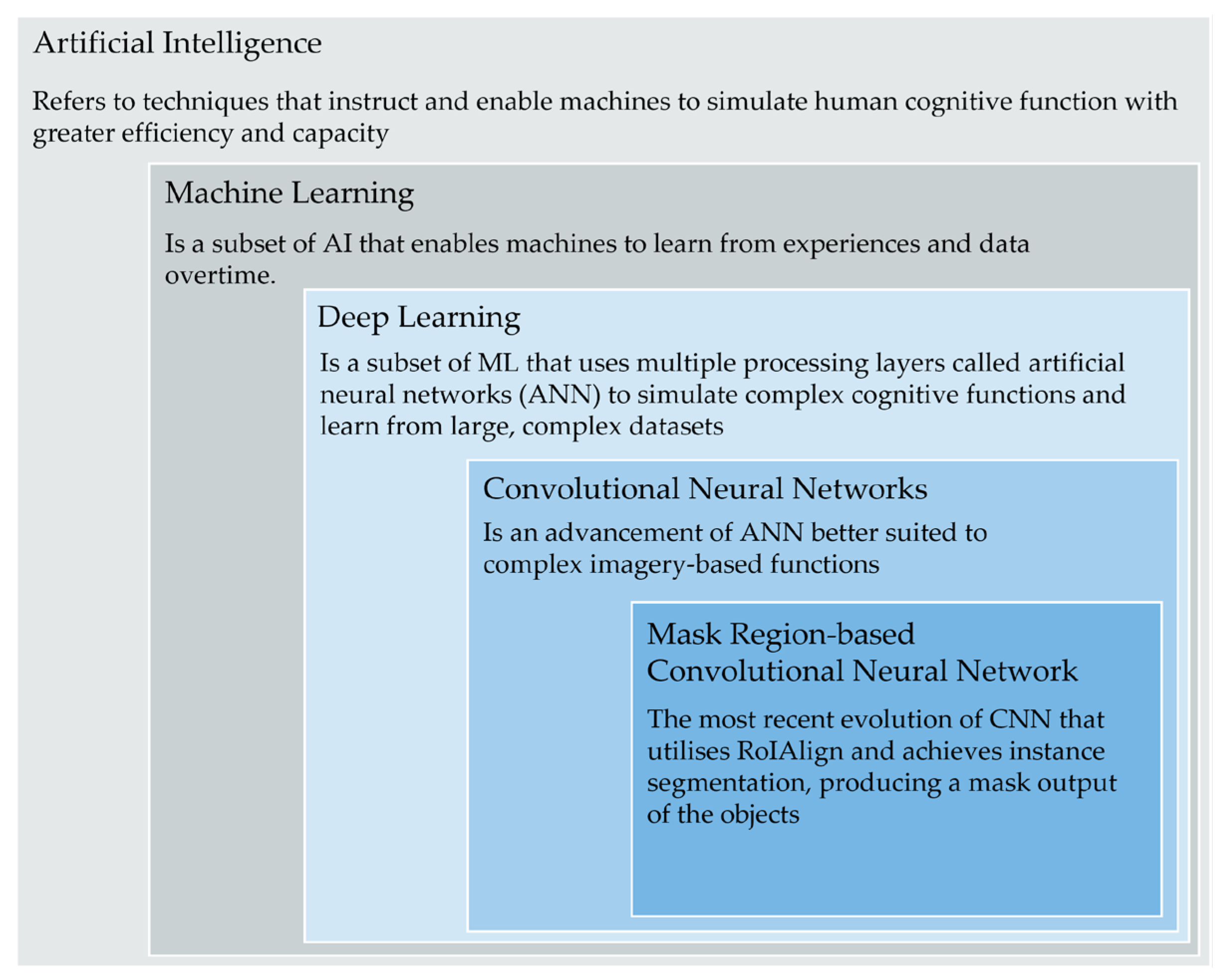
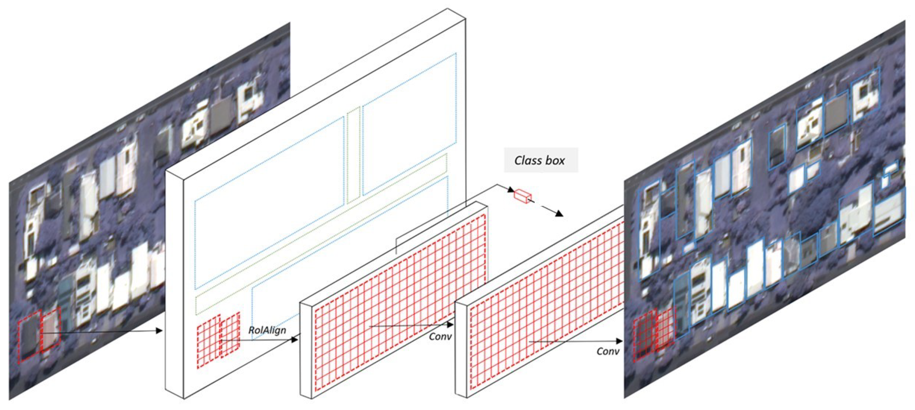
1.4. Mask Region-Based Convolutional Neural Network
1.5. Summary
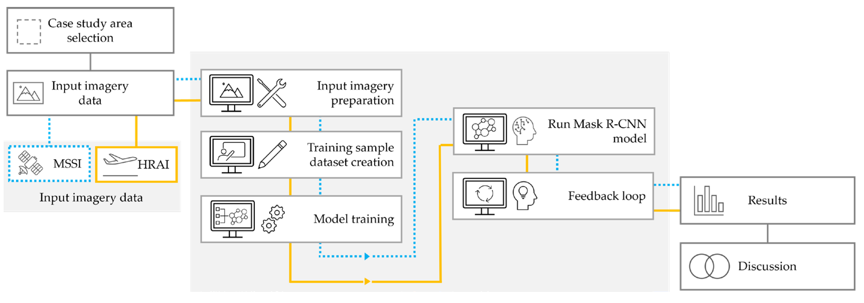
2. Methods
2.1. Overview
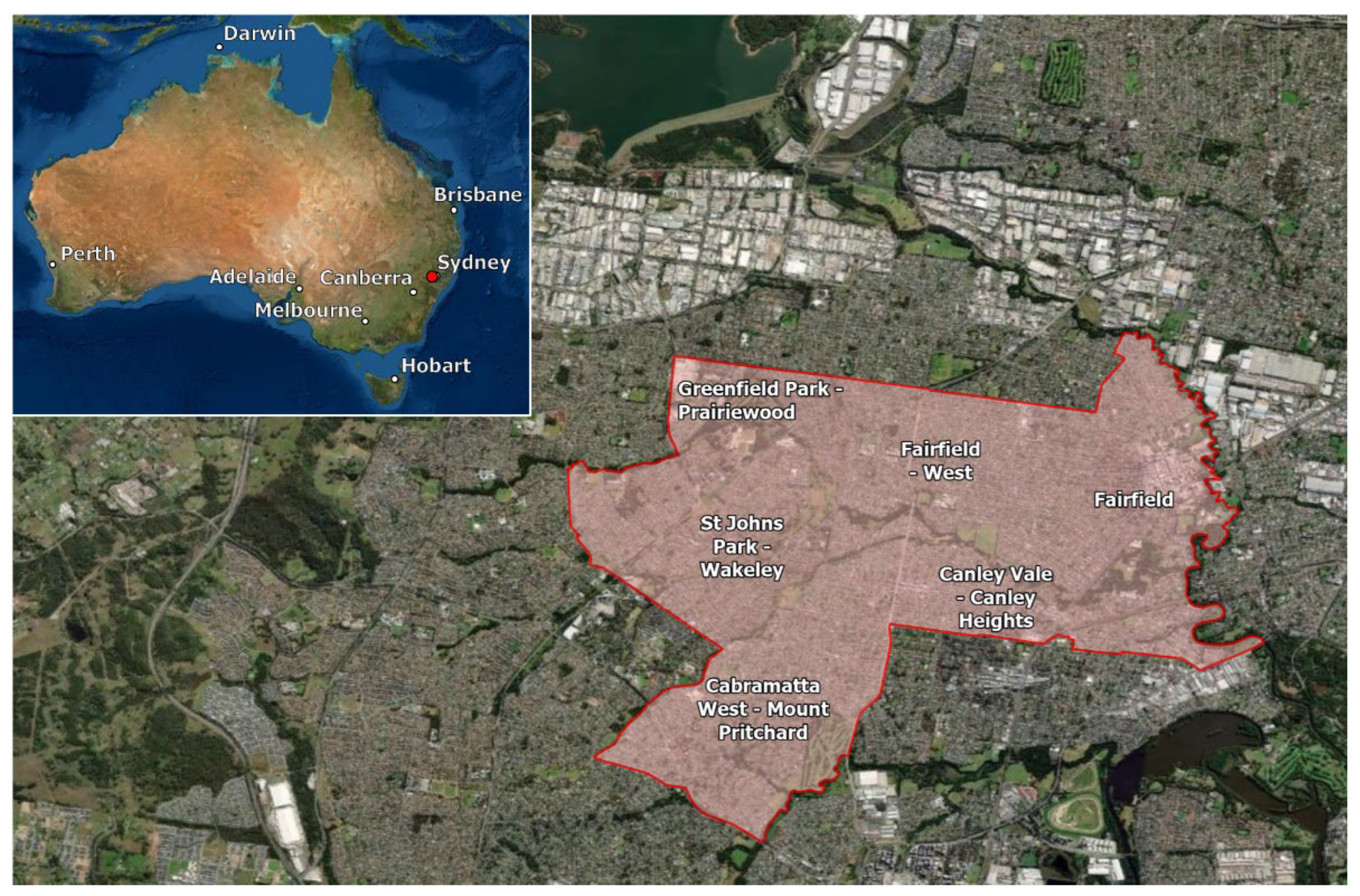
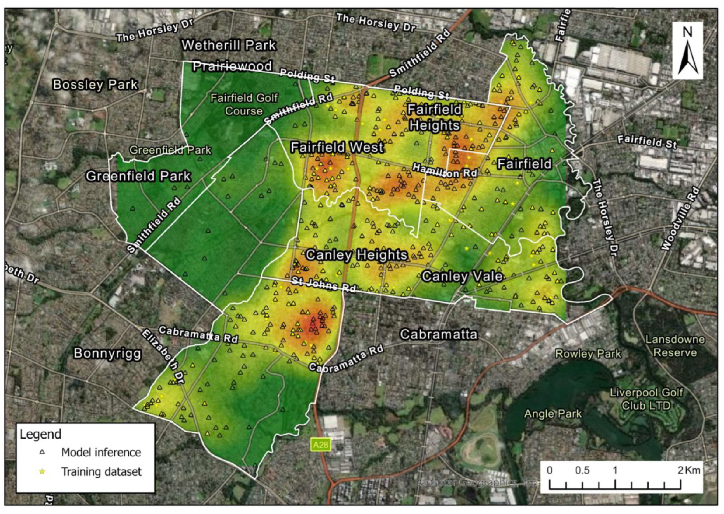
2.2. Case Study Area Selection
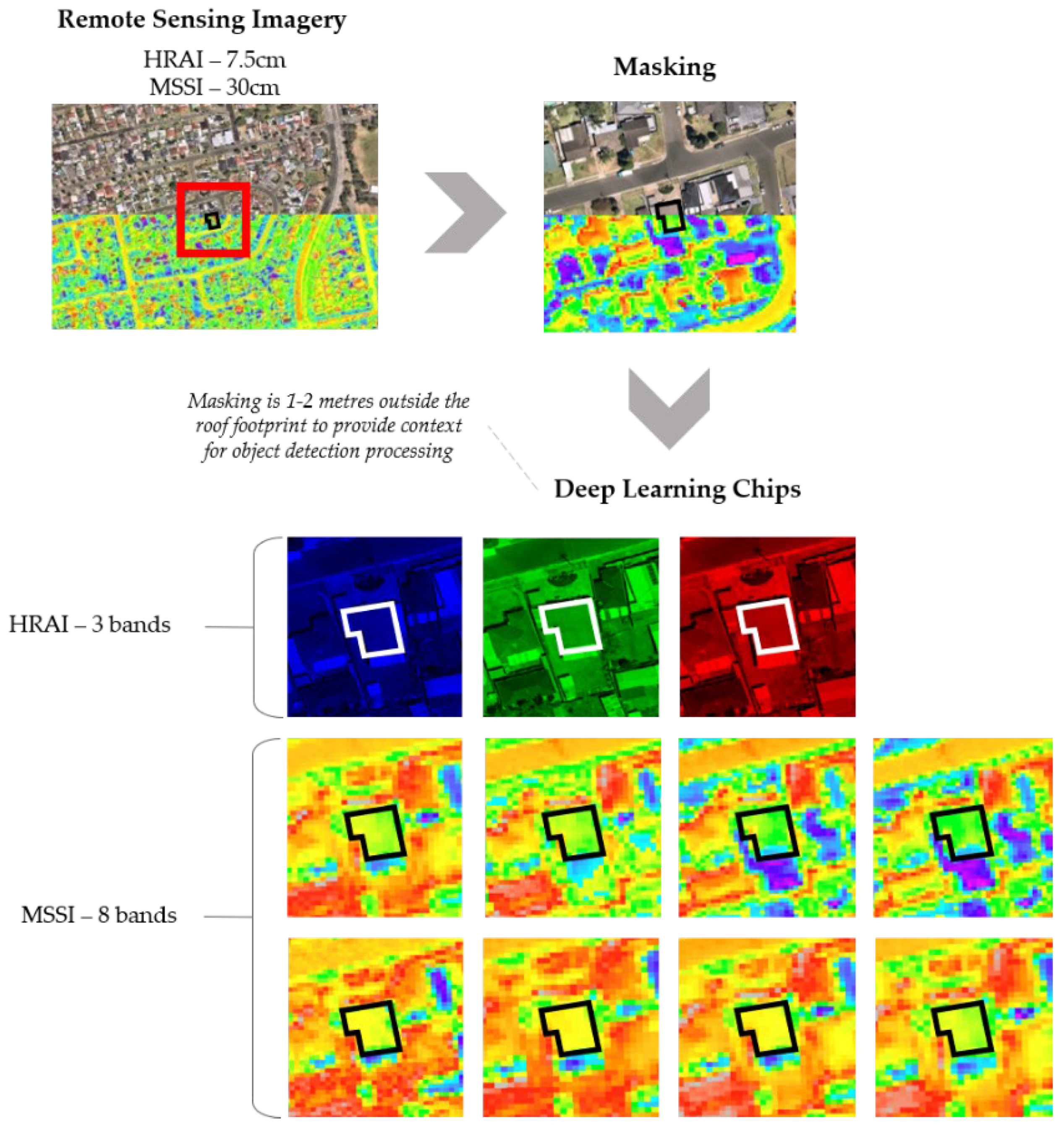
2.3. Input Imagery Data
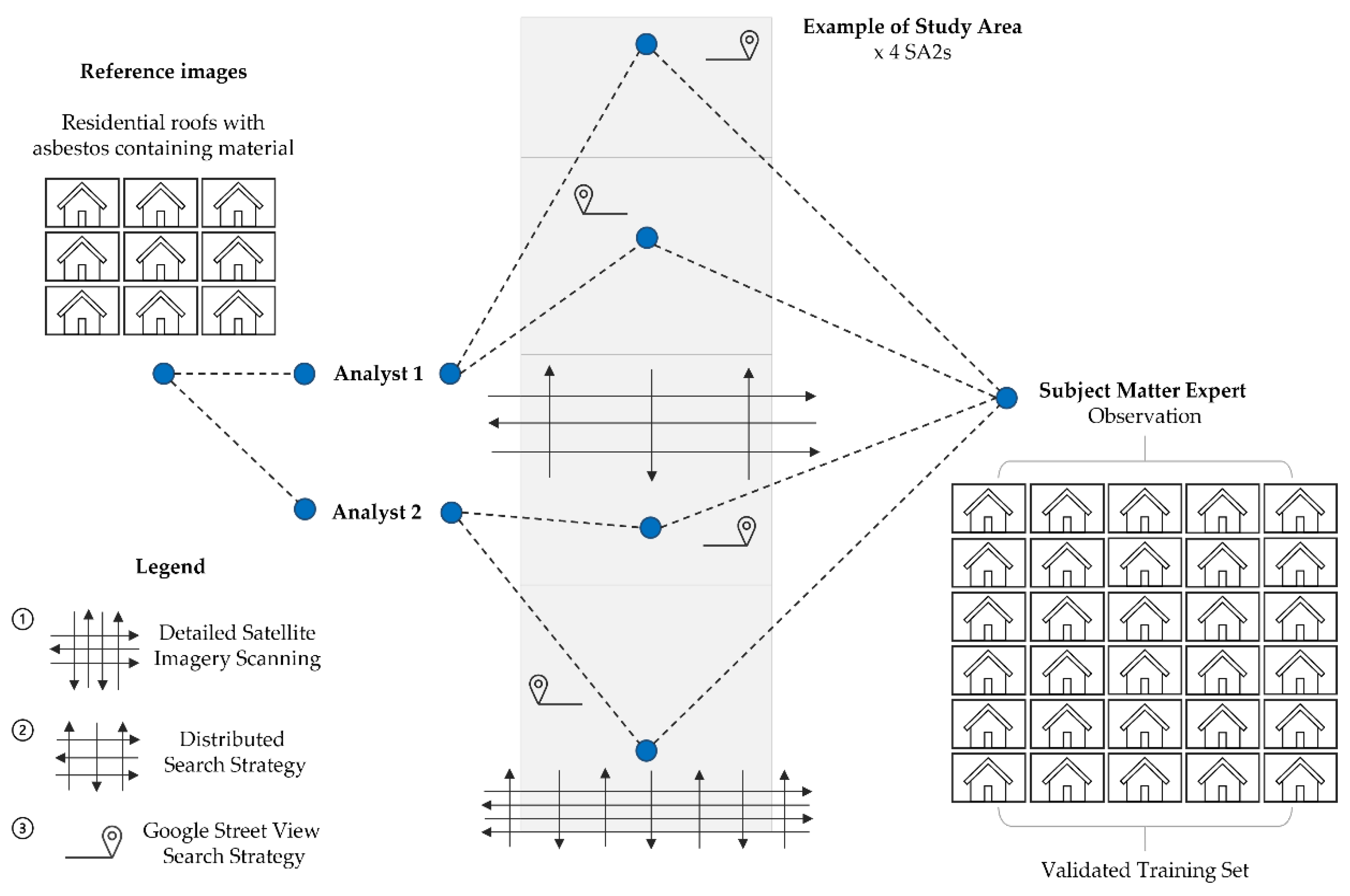
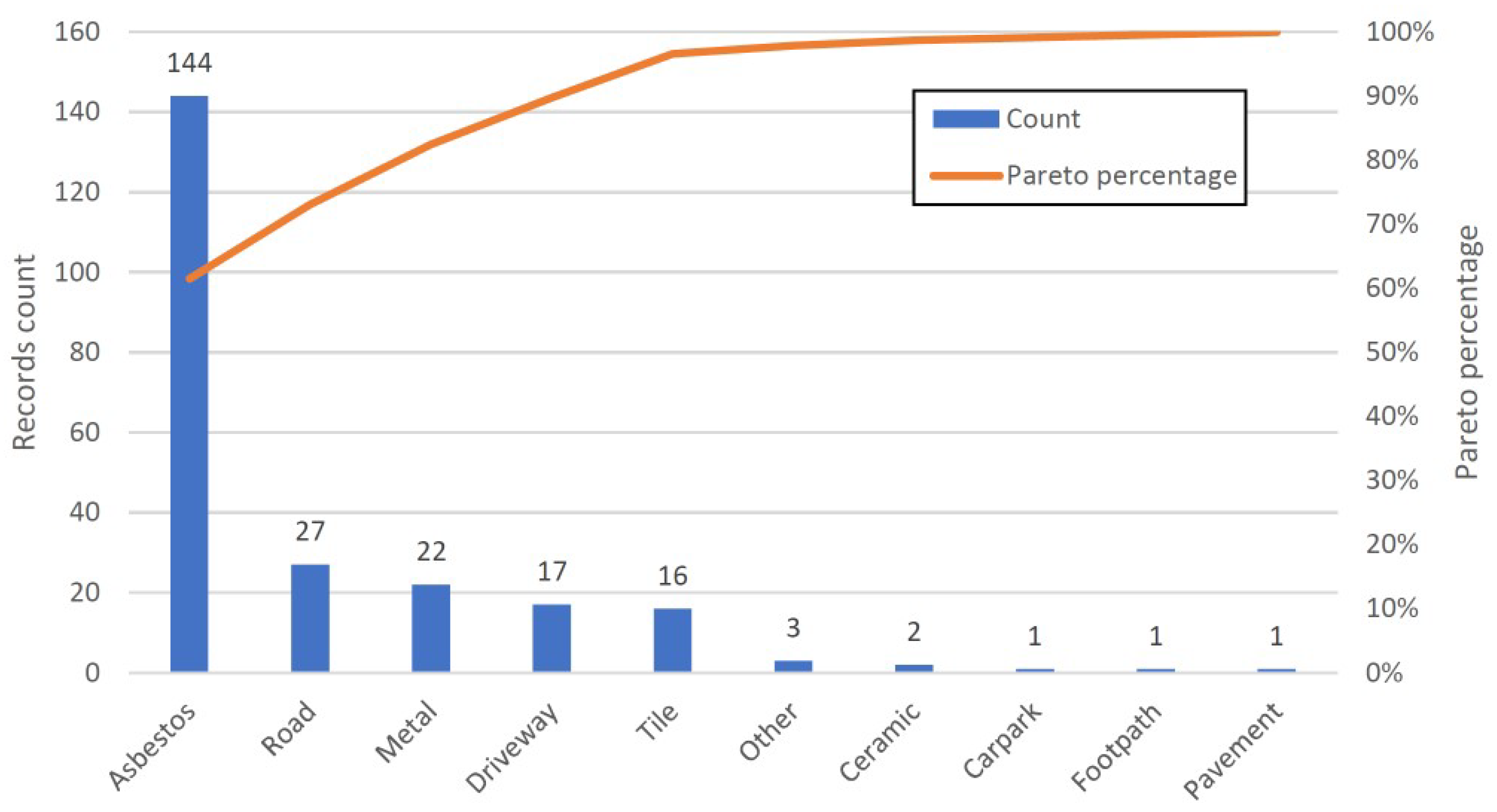
2.4. Training Sample Dataset Creation
- detailed aerial imagery searches scanning left to right across each urban block at different scales to identify different roofing materials depending on the imagery resolution,
- a more distributed search strategy to scan across a broader area to better observe patterns of streets and property sizes at a larger scale,
- ‘desktop-walking’ down the streets with ACM dwellings using Google Street-view to observe potential ACM roofing that could not be fully observed in aerial imagery.
2.5. Model Training
2.6. Run Mask R-CNN Model
2.7. Feedback Loop
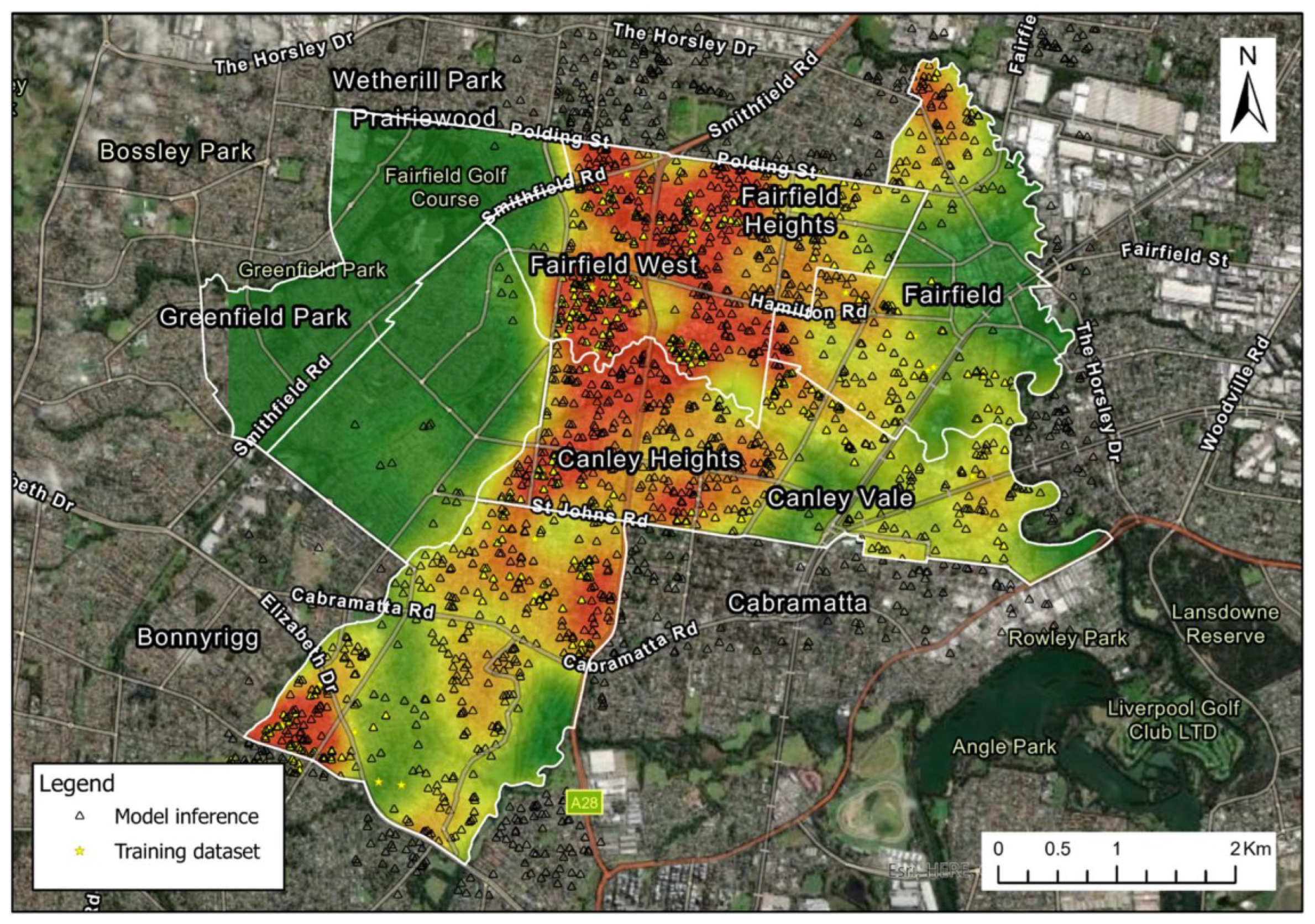
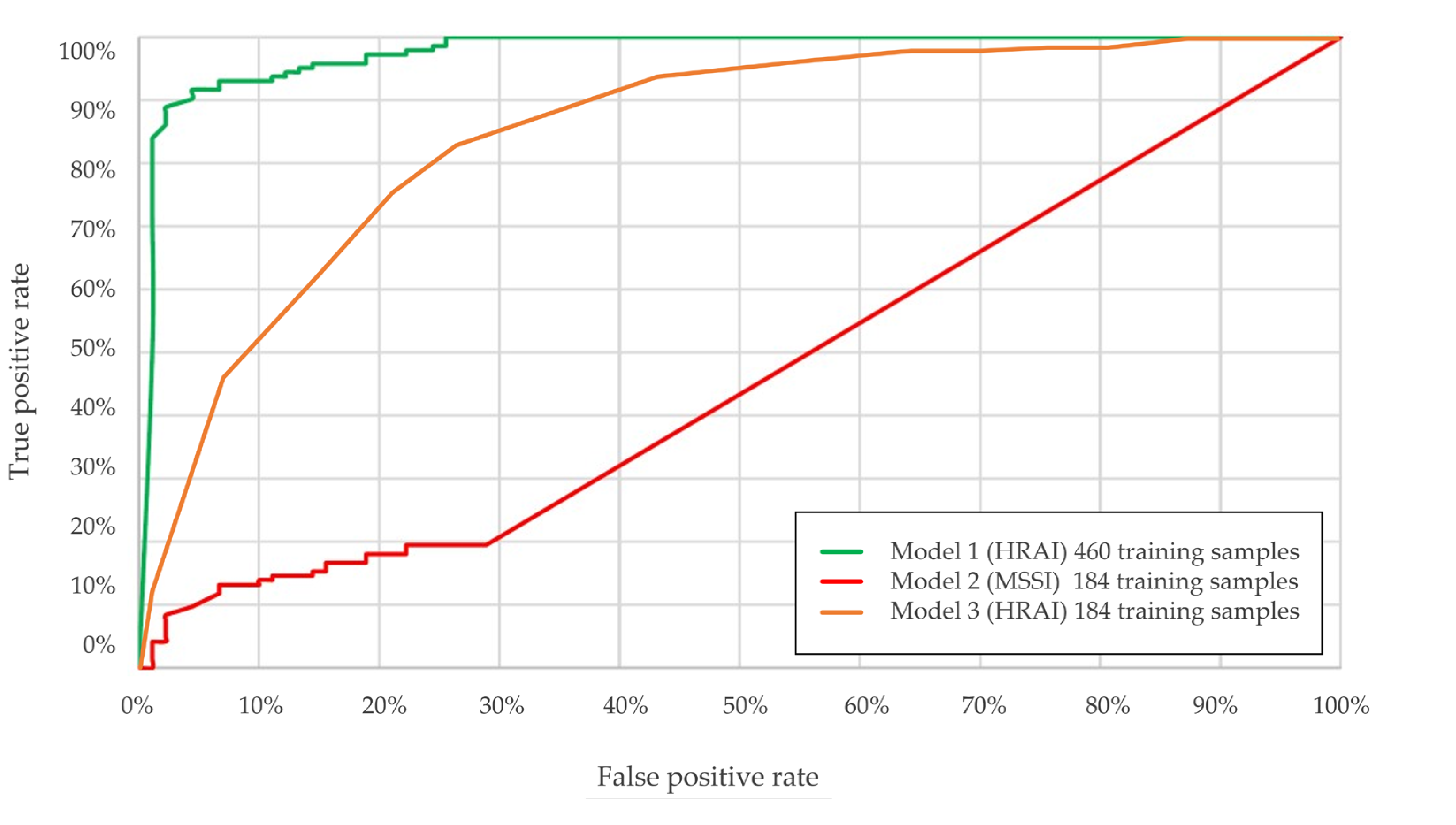
3. Results
4. Discussion
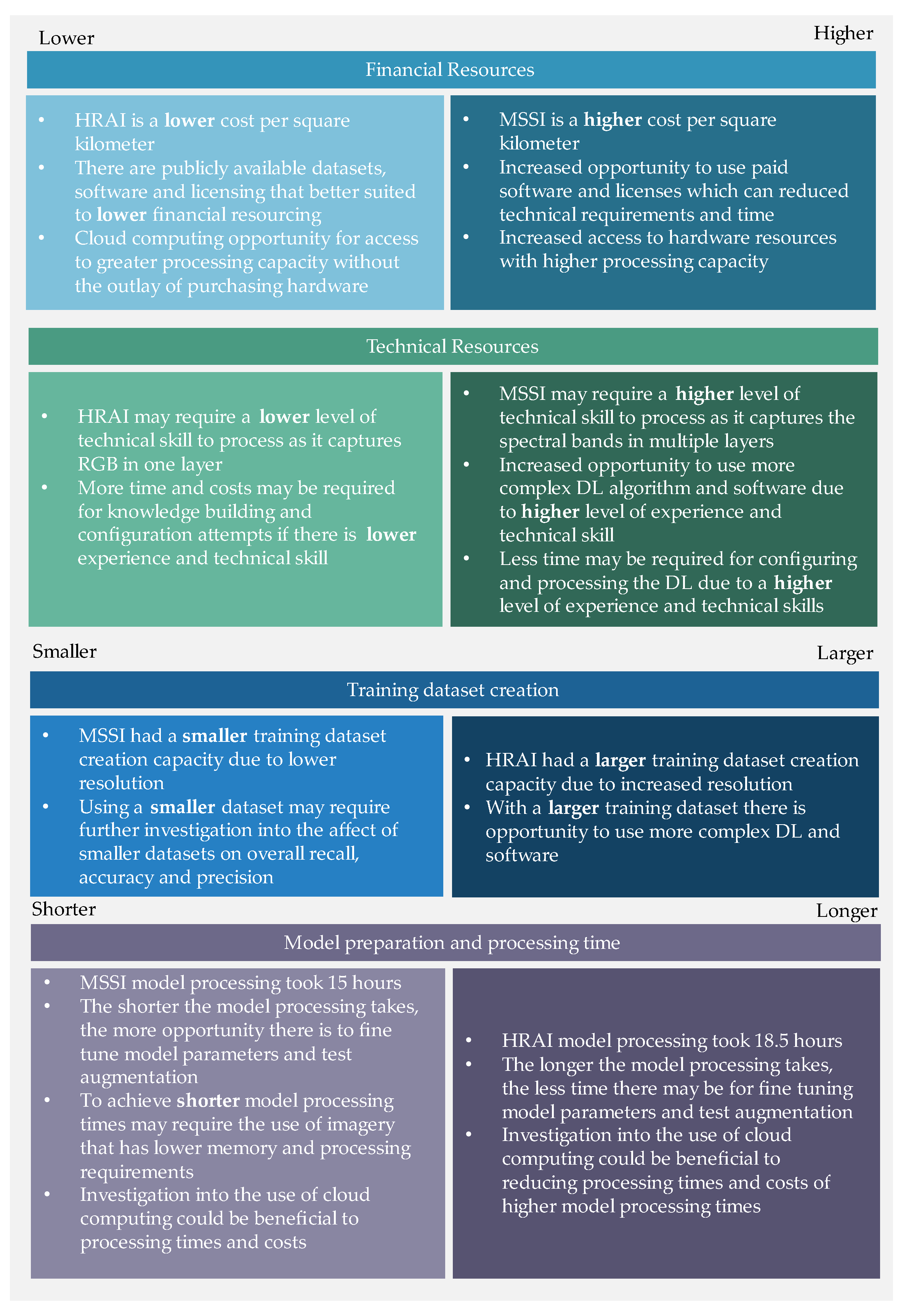
4.1. Financial and Technical Resources
4.2. Input Data Ownership and Usage Restrictions
4.3. Input Imagery Characteristics
4.4. Training Sample Dataset Creation and Size
4.5. Model Preparation and Processing Time
4.6. Application of Deep Learning
5. Conclusions
6. Future Research Direction
Author Contributions
Funding
Funding
Institutional Review Board Statement
Informed Consent Statement
Data Availability Statement
Conflicts of Interest
References
- Furuya, S.; Chimed-Ochir, O.; Takahashi, K.; David, A.; Takala, J. Global asbestos disaster. Int. J. Environ. Res. Public Health 2018, 15, 1000. [Google Scholar] [CrossRef] [PubMed] [Green Version]
- Frank, A. Global use of asbestos—Legitimate and illegitimate issues. J. Occup. Med. Toxicol. 2020, 15, 16. [Google Scholar] [CrossRef] [PubMed]
- International Agency for Research on Cancer (IARC). Arsenic, Metals, Fibres, and Dusts—Volume 100C Asbestos (Chrysotile, Amosite, Crocidolite, Tremolite, Actinolite, and Anthophyllite), in IARC Monographs on the Evaluation of Carcinogenic Risks to Humans. Available online: https://publications.iarc.fr/120 (accessed on 20 May 2022).
- Asbestos Safety and Eradication Agency (ASEA). National Asbestos Profile of Australia. 2017. Available online: https://www.asbestossafety.gov.au/sites/default/files/documents/2017-12/ASEA_National_Asbestos_Profile_interactive_Nov17.pdf (accessed on 11 May 2022).
- Asbestos Safety and Eradication Agency. Updated Asbestos Stocks and Flows Model. Available online: https://www.asbestossafety.gov.au/what-we-do/news-and-announcements/updated-asbestos-stocks-and-flows-model (accessed on 26 July 2022).
- Institute for Health Metrics and Evaluation. Global Burden of Disease (GBD). 2019. Available online: https://www.healthdata.org/gbd/gbd-2019-resources (accessed on 11 May 2022).
- Brown, B.; Hollins, I.; Pickin, J.; Donovan, S. Asbestos Stocks and Flows Legacy in Australia. Sustainability 2023, 15, 2282. [Google Scholar] [CrossRef]
- Abbasi, M.; Mostafa, S.; Vieira, A.S.; Patorniti, N.; Stewart, R.A. Mapping Roofing with Asbestos-Containing Material by Using Remote Sensing Imagery and Machine Learning-Based Image Classification: A State-of-the-Art Review. Sustainability 2022, 14, 8068. [Google Scholar] [CrossRef]
- Tommasini, M.; Bacciottini, A.; Gherardelli, M. A QGIS Tool for Automatically Identifying Asbestos Roofing. ISPRS Int. J. Geo-Inf. 2019, 8, 131. [Google Scholar] [CrossRef] [Green Version]
- Krówczyńska, M.; Raczko, E.; Staniszewska, N.; Wilk, E. Asbestos-cement roofing identification using remote sensing and convolutional neural networks (CNNs). Remote Sens. 2020, 12, 408. [Google Scholar] [CrossRef] [Green Version]
- Safe Work Australia. Model Work Health and Safety Regulations 2011, updated January 2021. Available online: https://www.safeworkaustralia.gov.au/doc/model-whs-regulations (accessed on 1 November 2022).
- Asbestos Safety and Eradication Agency. Asbestos in the Home. Available online: https://www.asbestossafety.gov.au/find-out-about-asbestos/asbestos-home (accessed on 11 May 2022).
- AS 4964-2004; Method for the Qualitative Identification of Asbestos in Bulk Samples. Standards Australia: Sydney, Australia, 2004. Available online: https://www.standards.org.au/standards-catalogue/sa-snz/other/ch-031/as-4964-2004 (accessed on 1 November 2022).
- Guo, W.; Yang, W.; Zhang, H.; Hua, G. Geospatial Object Detection in High-resolution Satellite Images Based on Multi-Scale Convolutional Neural Network. Remote Sens. 2018, 10, 131. [Google Scholar] [CrossRef] [Green Version]
- Zhang, L.; Zhang, L.; Du, B. Deep Learning for Remote Sensing Data. IEEE Xplore 2016, 4, 22–40. [Google Scholar]
- Bassani, C.; Maria, R.; Cavalcante, F.; Cuomo, V.; Palombo, A.; Pascucci, S.; Pignatti, S. Deterioration status of asbestos-cement roofing sheets assessed by analysing hyperspectral data. Remote Sens. 2017, 109, 361–378. [Google Scholar]
- Weih, R.C.; Riggan, N.D. Object-based classification vs. pixel-based classification: Comparative importance of multi-resolution imagery. ISPRS J. Photogramm. Remote Sens. 2008, 38, C7. [Google Scholar]
- Frassy, F.; Candiani, G.; Rusmini, M.; Maianti, P.; Marchesi, A.; Nodari, F.R.; Via, G.D.; Albonico, C.; Gianinetto, M. Mapping asbestos-cement roofing with hyperspectral remote sensing over a large mountain region of the Italian western alps. Sensors 2014, 14, 15900–15913. [Google Scholar] [CrossRef] [PubMed] [Green Version]
- Taherzadeh, E.; Shafri, H.Z.M. Development of a generic model for the detection of roof materials based on an object-based approach using WorldView-2 satellite imagery. Adv. Remote Sens. 2013, 2, 312–321. [Google Scholar] [CrossRef] [Green Version]
- Toth, C.; Jóźków, G. Remote sensing platforms and sensors: A survey. ISPRS J. Photogramm. Remote Sens. 2016, 115, 22–36. [Google Scholar] [CrossRef]
- Houborg, R.; Fisher, J.; Skidmore, A. Advances in remote sensing of vegetation function and traits. Int. J. App. Earth Obs. Geoinform. 2015, 43, 1–6. [Google Scholar] [CrossRef] [Green Version]
- Sarker, I. AI-Based Modeling: Techniques, Applications and Research Issues towards Automation, Intelligent and Smart Systems. SN Comput. Sci. 2022, 3, 158. [Google Scholar] [CrossRef]
- Iqbal, M.; Ali, H.; Tran, S.; Iqbal, T. Coconut trees detection and segmentation in aerial imagery using mask region-based convolution neural network. IET Comp. Vis. 2021, 15, 428–439. [Google Scholar] [CrossRef]
- Campbell, J.; Wynne, R. Introduction to Remote Sensing, 5th ed.; The Guildford Press: New York, NY, USA, 2011. [Google Scholar]
- Aerometrex. Key Factors to Consider When Choosing between Aerial and Satellite Imagery. Available online: https://aerometrex.com.au/resources/blog/key-factors-consider-when-choosing-between-aerial-satellite-imagery/ (accessed on 20 May 2022).
- Ose, K.; Corpetti, T.; Demagistri, L. Multispectral satellite image processing. In Optical Remote Sensing of Land Surface; Elsevier: Amsterdam, The Netherlands, 2016; pp. 57–124. [Google Scholar] [CrossRef]
- Apollo Mapping. High Resolution Satellite & Aerial Imagery. Available online: https://apollomapping.com/imagery/high-resolution-imagery (accessed on 21 May 2022).
- Digital Globe. Worldview-3. Available online: http://content.satimagingcorp.com.s3.amazonaws.com/media/pdf/WorldView-3-PDF-Download.pdf (accessed on 21 May 2022).
- Aerometrex. The Company. Available online: https://aerometrex.com.au/about/company/ (accessed on 2 August 2022).
- Nearmap. Current Aerial Maps Average. Available online: https://www.nearmap.com/au/en/current-aerial-maps-coverage (accessed on 2 August 2022).
- American Association for the Advancement of Science (AAAS). High Resolution Satellite Imagery Ordering and Analysis Handbook. Available online: https://www.aaas.org/resources/high-resolution-satellite-imagery-ordering-and-analysis-handbook (accessed on 20 May 2022).
- Harvey, M.; Pearson, S.; Alexander, K.; Rowland, J.; White, P. Unmanned aerial vehicles (UAV) for cost effective aerial orthophotos and digital surface models (DSM). In Proceedings of the New Zealand Geothermal Workshop, Auckland, New Zealand, 24–26 November 2014. [Google Scholar]
- Sarker, I. Deep Learning: A Comprehensive Overview on Techniques, Taxonomy, Applications and Research Directions. SN Comput. Sci. 2021, 2, 420. [Google Scholar] [CrossRef]
- Wang, D.; Liu, Z.; Gu, X.; Wu, W.; Chen, Y.; Wang, L. Automatic Detection of Pothole Distress in Asphalt Pavement Using Improved Convolutional Neural Networks. Remote Sens. 2022, 14, 3892. [Google Scholar] [CrossRef]
- Bharati, P.; Pramanik, A. Deep Learning Techniques—R-CNN to Mask R-CNN: A Survey. In Computational Intelligence in Pattern Recognition; Das, A., Nayak, J., Naik, B., Pati, S., Pelusi, D., Eds.; Springer: Singapore, 2019; Volume 999, pp. 657–668. [Google Scholar]
- Khanzode, C.A.; Sarode, R.D. Advantages and Disadvantages of Artificial Intelligence and Machine Learning: A Literature Review. Int. J. Lib. Inform. Sci. 2020, 9, 30–36. [Google Scholar]
- Hafiz, A.M.; Bhat, G.M. A survey on instance segmentation: State of the art. Int. J. Multimed. Inf. Retr. 2020, 9, 171–189. [Google Scholar] [CrossRef]
- Yu, K.; Hao, Z.; Post, C.J.; Mikhailova, E.A.; Lin, L.; Zhao, G.; Tian, S. Comparison of Classical Methods and Mask R-CNN for Automatic Tree Detection and Mapping Using UAV Imagery. Remote Sens. 2022, 14, 295. [Google Scholar] [CrossRef]
- 1270.0.55.001; Australian Statistical Geography Standard (ASGS): Volume 1—Main Structure and Greater Capital City Statistical Areas. Australia Bureau of Statistics: Canberra, Australia, 2016. Available online: https://www.abs.gov.au/ausstats/abs@.nsf/lookup/by%20subject/1270.0.55.001~july%202016~main%20features~statistical%20area%20level%202%20(sa2)~10014#:~:text=Their%20purpose%20is%20to%20represent,Australia%20without%20gaps%20or%20overlaps (accessed on 2 December 2021).
- Pinnegar, S.; Freestone, R.; Randolph, B. Suburban reinvestment through ‘knockdown rebuild’ in Sydney. In Suburbanization in Global Society (Research in Urban Sociology); Clapson, M., Hutchison, R., Eds.; Emerald Group Publishing Limited: Bingley, UK, 2010; pp. 205–229. [Google Scholar]
- Australia Bureau of Statistics Search Census Data. Available online: https://www.abs.gov.au/census/find-census-data/search-by-area (accessed on 2 December 2021).
- Gwyther, G. From Cowpastures to pigs’ heads: The development and character of western Sydney. Sydney J. 2008, 1, 51–74. [Google Scholar] [CrossRef] [Green Version]
- Fiumi, L.; Congedo, L.; Meoni, C. Developing expeditious methodology for mapping asbestos-cement roof coverings over the territory of Lazio Region. App. Geomat. 2014, 6, 37–48. [Google Scholar] [CrossRef]
- Xu, X.; Zhao, M.; Shi, P.; Ren, R.; He, X.; Wei, X.; Yang, H. Crack Detection and Comparison Study Based on Faster R-CNN and Mask R-CNN. Sensors 2022, 22, 1215. [Google Scholar] [CrossRef]
- Ramezan, C.A.; Warner, T.A.; Maxwell, A.E.; Price, B.S. Effects of Training Set Size on Supervised Machine-Learning Land-Cover Classification of Large-Area High-Resolution Remotely Sensed Data. Remote Sens. 2021, 13, 368. [Google Scholar] [CrossRef]
- Liu, Y.; Liu, J.; Pu, H.; Liu, Y.; Song, S. Instance Segmentation of Outdoor Sports Ground from High Spatial Resolution Remote Sensing Imagery Using the Improved Mask R-CNN. Int. J. Geosci. 2019, 10, 884–905. [Google Scholar] [CrossRef] [Green Version]
- Velásquez, N.; Estévez, E.C.; Pesado, P.M. Cloud computing, big data and the industry 4.0 reference architectures. J. Comp. Sci. Tech. 2018, 18, 258–266. [Google Scholar] [CrossRef]


| Attributes | MSSI | HRAI |
|---|---|---|
| Method of capture | Several photos of the same scene using different sensors attached to a satellite (see Figure 1B,D) [25]. | One photo taken of one scene until the desired area is covered using a high-resolution camera attached to an aerial vehicle (see Figure 1A,C) [24]. |
| Bands of the electromagnetic spectrum captured | Approximately 3 to 10 bands depending on the number of sensors. Bands can include red, green, blue (RGB), near-infrared, thermal infrared, short-wave infrared, panchromatic, cirrus and thermal infrared [26] | Three bands available: red, green, blue (RGB). |
| Available resolution | Three to four types of resolution are generally available.
| High to very high-resolution available ranging from 2.5 to 10–15 cm per pixel [25,27] |
| Weather | Generally, cannot guarantee cloud-free imagery, particularly over tropical areas. MSSI can be affected by atmospheric interference, which requires post-processing corrections [25]. | Flexible data capturing subject to the local weather, including altitude adjustments. This can guarantee cloud-free data and aerial imagery is not impacted by atmospheric interference [25]. |
| Location accuracy and accessibility | General accuracy is 10–20 m without ground control points, and accuracy is improving with new satellite technology [25]. | General horizontal accuracy is two pixels and the accuracy of aerial imagery is improving with the use of airborne ground positioning systems and post-processing. |
| Speed | Generally, capturing specific locations and time-sensitive events cannot be guaranteed within two to three days, as they are depending on the satellite’s position in orbit. Worldview-3 has an average revisit time of less than one day [28]. MSSI processing times are low as there is usually a smaller number of images to process due to the coverage. | HRAI is useful for specific locations or time-sensitive events depending on the availability of the equipment to the location. Processing times for this imagery are dependent on the number of images captured for coverage. This is improving with advancements in technology [25]. |
| Coverage and currency | MSSI can quickly cover large geographic areas when in the correct place. Worldview-3 can cover up to 680,000 km2 per day [28]. | HRAI can capture large amounts of data in a small quantity of data collection runs. Commercial aerial imagery providers in Australia update the coverage of metropolitan areas 2–6 times a year and can provide access up to 3900 to 130,100 per km2 [29,30]. |
| Cost | Varies depending on resolutions, accuracy and timeliness. Worldview-1 and Worldview-2 cost anywhere between AUD$14 1 and AUD$23 1 per km2 depending on the currency [27,31] | Varies depending on mobilisation costs, resolution, accuracy, timeliness and if manned or unmanned [25]. Commercial suppliers can charge AUD$5.91 1 per km2 for 15 cm resolution, archived, orthorectified, aerial imagery captured by a manned aerial vehicle [27]. Unmanned aerial vehicles (UAV) capture, such as using drones, can lower associated costs [32]. |
| Author | Resolution (Metres) | Bands | Capture |
|---|---|---|---|
| Weih and Riggan (2008) [17] | 1 m | 11 | Aerial & satellite |
| 1 m | 7 | Aerial & satellite | |
| 10 m | 8 | Satellite | |
| Bassani et al. (2007) * [16] | 3 m | 102 (hyperspectral) | Aerial |
| Frassy et al. (2014) * [18] | 4 m | 102 (hyperspectral) | Aerial |
| 6 m–9 m | 102 (hyperspectral) | Aerial | |
| Taherzadeh and Shafri (2013) * [19] | 0.5 m | 8 (visible and near-infrared) | Satellite |
| Guo et al. (2018) [14] | 0.5 m–2 m | 3 (RGB) | Satellite |
| 0.08 m | 2 (colour-infrared) | Satellite | |
| Krówczyńska et al. (2020) * [10] | 0.25 m | 5 (RBG & colour-infrared) | Aerial |
| Method | Format | Model | Data Created |
|---|---|---|---|
| Training Dataset Creation | |||
| Used SME observations, desktop analysis and imagery to outline potential ACM roofing locations | Polygon shapefile | Model 1 | 460 polygons of ACM roofing locations |
| Model 2 | 184 polygons of ACM roofing locations | ||
| Model 3 | 184 polygons of ACM roofing locations | ||
| Model training | |||
| Created ‘chips’ of imagery from the locations of the training dataset creation step and used them to train the model. | Tag Image Film Format (TIFF) | Model 1 | HRAI 7.5 cm resolution chips of ACM roofs |
| Model 2 | MSSI 30 cm resolution chips of ACM roofs | ||
| Model 3 | HRAI 7.5 cm resolution chips of ACM roofs | ||
| Model Parameters | Model 1—HRAI | Model 2—MSSI |
|---|---|---|
| Case Study Area Details | ||
| Area | Western Sydney | Western Sydney |
| Included SA2s | Cabramatta West—Mount Prichard, Canley Vale—Canley Heights, Fairfield, Fairfield—West, Greenfield Park—Prairiewood, St. Johns Park—Wakeley | Cabramatta West—Mount Prichard, Canley Vale—Canley Heights, Fairfield, Fairfield—West, Greenfield Park—Prairiewood, St. Johns Park—Wakeley |
| Population (2016) [41] | 93,944 | 93,944 |
| Dwelling Count (2016) [41] | 29,595 | 29,595 |
| Area (km2) (2016) [41] | 26.8 | 26.8 |
| Model input | ||
| Model type | Mask R-CNN | Mask R-CNN |
| Training sample size | 460 | 184 |
| Input imagery resolution | 7.5 cm | 30 cm & 1.24 m |
| Input imagery band types | 3 (RGB) | 8 (RGB, red-edge, coastal, near-infrared 1, near-infrared 2 & panchromatic) |
| Input imagery pre-processing | N/A | Pan-sharpening |
| Model processing | ||
| Processing unit | Graphics processing unit (GPU) | Graphics processing unit (GPU) |
| Processing time | 15 h | 18 h 30 min |
| Model output | ||
| Confidence threshold | 99.8% | 90% |
| Recall rate (inferences) | 1938 | 533 |
| Average precision | 94% | 63% |
| Model Parameters | Model 2—MSSI | Model 3—HRAI |
|---|---|---|
| Model Input | ||
| Model type | Mask R-CNN | Mask R-CNN |
| Training dataset size | 184 | 184 |
| Input imagery resolution | 30 cm & 1.24 m | 7.5 cm |
| Input imagery band types | 8 (RGB, red-edge, coastal, near-infrared 1, near-infrared 2 & panchromatic) | 3 (RGB) |
| Input imagery pre-processing | Pan-sharpening | N/A |
| Model processing | ||
| Processing unit | Graphics processing unit (GPU) | Graphics processing unit (GPU) |
| Processing time | 15 h | 10 h |
| Model output | ||
| Confidence threshold | 90% | 98% |
| Recall rate (inferences) | 533 | 1737 |
| Average precision | 63% | 62% |
Disclaimer/Publisher’s Note: The statements, opinions and data contained in all publications are solely those of the individual author(s) and contributor(s) and not of MDPI and/or the editor(s). MDPI and/or the editor(s) disclaim responsibility for any injury to people or property resulting from any ideas, methods, instructions or products referred to in the content. |
© 2023 by the authors. Licensee MDPI, Basel, Switzerland. This article is an open access article distributed under the terms and conditions of the Creative Commons Attribution (CC BY) license (https://creativecommons.org/licenses/by/4.0/).
Share and Cite
Hikuwai, M.V.; Patorniti, N.; Vieira, A.S.; Frangioudakis Khatib, G.; Stewart, R.A. Artificial Intelligence for the Detection of Asbestos Cement Roofing: An Investigation of Multi-Spectral Satellite Imagery and High-Resolution Aerial Imagery. Sustainability 2023, 15, 4276. https://doi.org/10.3390/su15054276
Hikuwai MV, Patorniti N, Vieira AS, Frangioudakis Khatib G, Stewart RA. Artificial Intelligence for the Detection of Asbestos Cement Roofing: An Investigation of Multi-Spectral Satellite Imagery and High-Resolution Aerial Imagery. Sustainability. 2023; 15(5):4276. https://doi.org/10.3390/su15054276
Chicago/Turabian StyleHikuwai, Mia V., Nicholas Patorniti, Abel S. Vieira, Georgia Frangioudakis Khatib, and Rodney A. Stewart. 2023. "Artificial Intelligence for the Detection of Asbestos Cement Roofing: An Investigation of Multi-Spectral Satellite Imagery and High-Resolution Aerial Imagery" Sustainability 15, no. 5: 4276. https://doi.org/10.3390/su15054276