Article

Coupling a Distributed Time Variant Gain Model into a Storm Water Management Model to Simulate Runoffs in a Sponge City

1
State Key Laboratory of Eco-Hydraulics in Northwest Arid Region, Xi’an University of Technology, Xi’an 710048, China
2
PowerChina Guiyang Engineering Corporation Limited, Guiyang 550081, China
3
State Key Laboratory of Water Resources and Hydropower Engineering Science, Wuhan University, Wuhan 430072, China
*
Author to whom correspondence should be addressed.
Sustainability 2023, 15(4), 3804; https://doi.org/10.3390/su15043804
Submission received: 16 January 2023 / Revised: 10 February 2023 / Accepted: 13 February 2023 / Published: 20 February 2023
(This article belongs to the Section Sustainable Urban and Rural Development)

Abstract

:
The storm water management model (SWMM) has been used extensively to plan, implement, control, and evaluate low impact development facilities and other drainage systems to solve storm-related problems in sponge cities. However, the calibration of SWMM involves a variety of sensitive parameters and may bring significant uncertainties. Here we incorporated the distributed time variant gain model (DTVGM), a model with a simple structure and few parameters, into the SWMM (called DTVGM-SWMM) to reduce the complexity but keep the mechanistic representation of the hydrological process. The DTVGM runoff module parameters were calibrated and validated using the Nash–Sutcliffe efficiency (NSE), based on measured data and the results of SWMM. It was then coupled with the SWMM routing module to estimate catchment runoffs and outflows. Finally, the performance was evaluated using NSE (0.57~0.94), relative errors of the flow depth (−7.59~19.79%), and peak flow rate (−33.68~54.37%) under different storm events. These implied that the DTVGM-SWMM simulations were generally consistent with those of the control group, but underperformed in simulating peak flows. Overall, the proposed framework could reasonably estimate the runoff, especially the outflow process in the urban catchment. This study provides a simple and reliable method for urban stormwater simulation.

1. Introduction

Rapid urbanization has caused various problems in constructed areas [1]. Increased surface runoff, frequent flooding, and water deterioration have significantly impacted the environment and the economy [2,3]. In the last decade, the Chinese government has launched sponge city construction [4], which often uses low impact development facilities (LIDs) as source control measurements [5]. A sponge city is a city with low impact development infrastructure, which aims to make the catchment hydrological response approach the pre-development status with minimum cost. In sponge cities, the runoff response to rainfall has significant nonlinear characteristics, which can be depicted by the storm water management model (SWMM), widely used in urban hydrology [6,7,8]. However, SWMM requires many parameters and much measured data; moreover, it operates in a complicated way.
On the other hand, the distributed time variant gain model (DTVGM) has few parameters and a simple structure for representing the rainfall-runoff response [9,10]. It can simulate complex nonlinear hydrological processes, but is generally used in large natural watersheds with low-intensity human activities under prolonged rainfalls. Thus far, DTVGM has rarely been used to simulate the rainfall runoff process in sponge cities as urban areas always have small areas, complicated land use and land cover, and, in most cases, short and intense storms. It would be questionable to apply it to a study subject with a small spatiotemporal scale [11]. Moreover, a direct reason for its rare usage is that DTVGM lacks a routing module for the drainage networks, which the SWMM can provide (written in C).
To this end, we aim to incorporate the runoff module of DTVGM into the routing module of SWMM for developing the DTVGM-SWMM to predict the runoff and outflow in a sponge city. The proposed model will contribute to the modeling and management of the rainfall-runoff process in sponge cities. This article is organized as follows: Section 2 presents the study area and data; Section 3 introduces the SWMM, DTVGM runoff module, coupling method, and performance indicators; Section 4 presents the results and a discussion from four perspectives; Section 5 summarizes the conclusions.

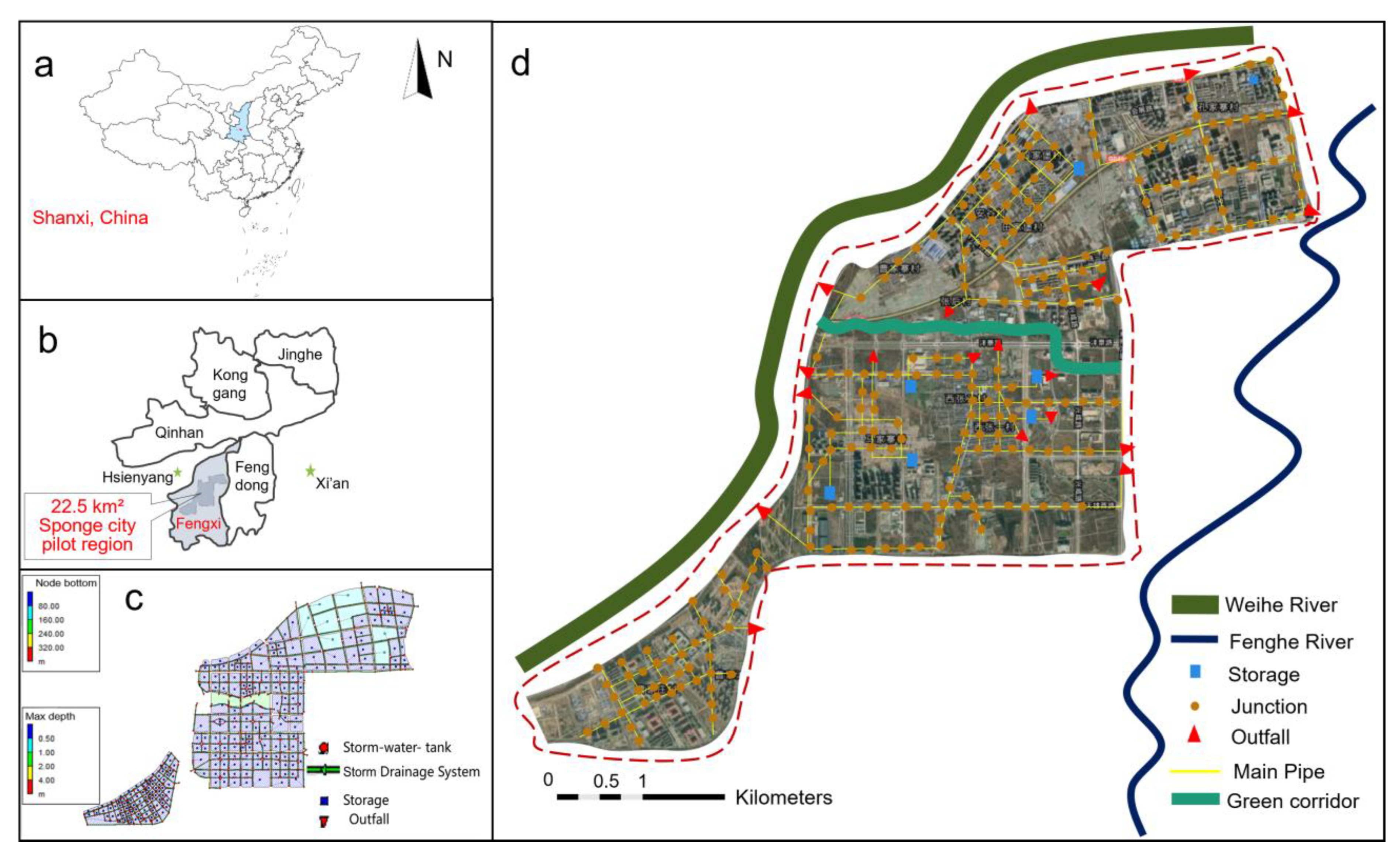
2. Study Area and Data

Fengxi New City is located between Xi’an and Xianyang (Figure 1b), Shaanxi Province, China (Figure 1a), with a total area of 143 km2. Since 2013, the study area (22.5 km2, Figure 1d) has been developed with a LID-based stormwater management system (Figure 1c). Fengxi was designated one of China’s pilot sponge cities in 2015 and a UNESCO global eco-hydrology demonstration site in 2019 (http://ecohydrology-ihp.org/demosites/view/1220 (accessed on 16 January 2023)), for featuring a temperate continental monsoon climate and nonself-weight collapsible loess land cover. The average annual temperature is about 13.6 °C, and the average annual rainfall depth is about 520.0 mm. Precipitation is mainly concentrated from July to September (50–60% of the annual amount), resulting in severe summer floods. The land cover includes built areas, roads, grasses, trees, bare grounds, water, etc. The study area has an average slope of 0.5%, with an elevation of 378.0–392.0 m, and outflows from outfalls are drained to the Weihe River and Fenghe River.
Most of the study area data, including measured rainfall and runoff data and the input file for SWMM, was provided by the Fengxi New City Management Committee; other data were collected or measured by our group. Table 1 lists the statistics of the storm events used to calibrate and validate the models.

3. Methodology

We ran the DTVGM and SWMM in the study area to account for rainfall-runoff heterogeneity between subcatchments (i.e., grid cells) within the catchment. A framework for coupling the DTVGM and SWMM was proposed to simulate runoffs and outflows in sponge cities (Figure 2). The flowchart consists of four parts: (1) the preprocessing and splitting of the observed storm events, including design storms and corresponding simulated flows, into a calibration group and a validation group; (2) calibration and validation of the SWMM model to simulate the rainfall runoff in subcatchments under storm events; (3) calibration of the DTVGM runoff module using a genetic algorithm [13]; (4) coupling the calibrated DTVGM runoff module with the SWMM routing module to develop the DTVGM-SWMM; (5) evaluating the coupling model using performance matrices.

3.1. Storm Water Management Model

SWMM is a widely used rainfall-runoff model developed by the US Environmental Protection Agency (https://www.epa.gov/water-research/storm-water-management-model-swmm (accessed on 16 January 2023)). The software consists of hydrological, hydrodynamic, and water quality modules and helps predict runoff quantity and quality from LIDs and drainage systems. It is free, open-source, and allows for the easy achievement of secondary development [14].
Based on the topography and underlying conditions, the study area was divided into 268 subcatchments (Figure 1c). In this paper, the SWMM model has 603 nodes, 603 sections of pipeline, and 25 outfalls (Figure 1d). Table 2 lists the values of the options and main hydrological parameters of SWMM [12,15]. Note that the SWMM used here was calibrated and validated with measured data, i.e., Event-20170820, Event-20170909, and Event-20170916.
Table 2. Values of options and main calibrated parameters for the storm water management model.
Options or ParametersValue 1
Infiltration modelHorton [16,17,18]
Routing modelDynwave [6,19,20,21,22,23,24,25,26,27]
Reporting time step (minute)1
Routing time step (second)10
Catchment slope (%)0.5
Imperviousness (%)65.0
Percent of the impervious area with no depression storage (%)35.0
Depression storage in impervious areas (mm)2.1
Depression storage in pervious areas (mm)3.6
Conduit roughness (s/m1/3)0.013
Surface roughness for overland flow in impervious area (s/m1/3)0.013
Surface roughness for overland flow in pervious area (s/m1/3)0.150
Minimum infiltration rate on Horton curve (mm/h)3.56
Maximum infiltration rate on Horton curve (mm/h)25.40
Decay rate constant of Horton curve (1/h)7
Drying time (day)7
1 Data from Yang et al. [12,28]. For more details on SWMM, please refer to Rossman [29,30].

3.2. Runoff Module of Distributed Time Variant Gain Model

The DTVGM divides the catchment into cell grids (i.e., subcatchments) based on GIS/DEM and applies the time variant gain model, a conceptual hydrological model, to each cell grid for runoff and routing calculations. Previous studies have shown that the DTVGM can perform well in large watersheds under prolonged rainfalls. In this section, we only explain the runoff module of DTVGM because the routing module of DTVGM is not used.
The number of grids in the DTVGM equals the number of subcatchments in the SWMM. For the ith subcatchment at time t, the runoff (Ri(t), mm) is the sum of the surface runoff ( R i S ( t ) , mm) and subsurface runoff ( R i S S ( t ) , mm). The surface runoff yielded in the subcatchment is calculated thus:
R i S ( t ) = G i ( t ) P i ( t )
where Pi(t) is the rainfall depth in the ith subcatchment at time t, mm. Gi(t) is the time variant gain factor (determined by soil moisture) in the ith subcatchment at time t:
G i ( t ) = g i 1 + g i 2 A P I i ( t )
where g i 1 and g i 2 are dimensionless time variant gain parameters of surface runoff for the ith subcatchment. APIi(t) is the antecedent precipitation index of the ith subcatchment at time t, which represents the recent soil moisture state of the subcatchment, mm [31,32,33]:
A P I i ( t ) = j = 1 t ( 1 e 1 K i ) e j K i P i ( t j + 1 )
where j is the time and t is the number of times; Ki, the dimensionless decay factor and is related to the soil property and evaporation within the ith catchment.
Lastly, for the ith subcatchment at time t, the subsurface runoff is calculated as:
R i S S ( t ) = g i 3 A P I i ( t )
where g i 3 is the dimensionless time variant gain parameter of subsurface runoff for the ith subcatchment.

3.3. Coupling Model

Though a monitoring system has been developed at a few sites in the catchment, there were no observed rainfall, runoff, and outflow data at a subcatchment scale. Thus, we calibrated the DTVGM runoff module using the genetic algorithm (https://ww2.mathworks.cn/help/gads/ga.html (accessed on 16 January 2023)) based on the subcatchments’ runoff time series calculated by SWMM. For the ith subcatchment, the decision variables of the optimization problem are g i 1 , g i 2 , g i 3 , and K i . Thus, we set the number of iterations to 8000, namely, 2000 times the number of decision variables.
The Nash-Sutcliffe efficiency (NSE) [28,34,35,36,37,38,39] was used to quantify the overall consistency between the hydrographs by DTVGM and observed values (including some hydrographs by SWMM). Note that NSE ranges from to 1, being equal to 1 if a perfect agreement exists. It is calculated as follows:
N S E i = 1 t = 1 N [ R i S W M M ( t ) R i D T V G M ( t ) ] 2 t = 1 N [ R i S W M M ( t ) R i S W M M ¯ ] 2
where N refers to the number of time steps of the runoff time series, min; Q i S W M M ( t ) and Q i D T V G M ( t ) are the runoff time series simulated by SWMM and DTVGM for the ith subcatchment at time step t, respectively, m3/s; Q i S W M M ¯ is the average value of runoff time series simulated by SWMM for the ith subcatchment, m3/s.
The objective function is to maximize the NSE value for the ith subcatchment. Here, the calibration was conducted 30 times, thus obtaining 30 sets of optimal parameters (decision variables) with corresponding NSE values. Thus, the optimization model for the calibration can be expressed as follows:
f i ( g i 1 , g i 2 , g i 3 , K i ) = m i n ( N S E i )
subject to:
1 g i 1 1 0 g i 2 2 0 g i 3 1 0 K i 100
Generally, developing a DTVGM-SWMM consists of three steps: (1) call the MATLAB engine (https://www.mathworks.com/help/matlab/calling-matlab-engine-from-c-programs-1.html?s_tid=CRUX_lftnav (accessed on 16 January 2023)) in Visual Studio (https://visualstudio.microsoft.com/ (accessed on 16 January 2023)) to run the runoff module of DTVGM that was developed in MATLAB by our group; (2) use the runoff results of DTVGM to replace the values of vOutflow in SWMM, which is a variable that refers to the rate of flow leaving from the catchment; (3) run the SWMM routing module to obtain catchment outflow time series.

3.4. Performance Criteria

We used three indicators, namely, the NSE (Equation (5)), the relative error of runoff depth ( δ R , Equation (8)), and that of peak runoff ( δ P , Equation (9)) to evaluate the coupling model. A higher NSE and a lower δR and δP indicate better performance. As defined in Equations (8) and (9), the values of δR and δP are positive when the DTVGM overestimates and are negative when it underestimates.
δ R ( i ) = [ R i D T V G M R i S W M M R i S W M M ] × 100 %
δ P ( i ) = [ m a x 1 t N R i D T V G M ( t ) m a x 1 t N R i S W M M ( t ) m a x 1 t N R i S W M M ( t ) ] × 100 %

4. Results and Discussion

4.1. Simulation of Storm Water Management Model

The relevant parameters of SWMM were adjusted; for details on the calibration and validation, please refer to Yang et al. [12]. In addition, we used a runoff coefficient-based method to verify the SWMM parameters. Theoretically, the integrated runoff coefficient for the study catchment is 0.45~0.60 because the site is densely built-up [40]. In fact, under Event-20170820, the subcatchment runoff coefficients calculated by the SWMM simulation were 0.52–0.57 for the no LIDs scenario and 0.18–0.28 for the LIDs scenario. Thus, the calibrated SWMM is satisfactory for calibrating and validating the DTVGM runoff module and the coupling model.

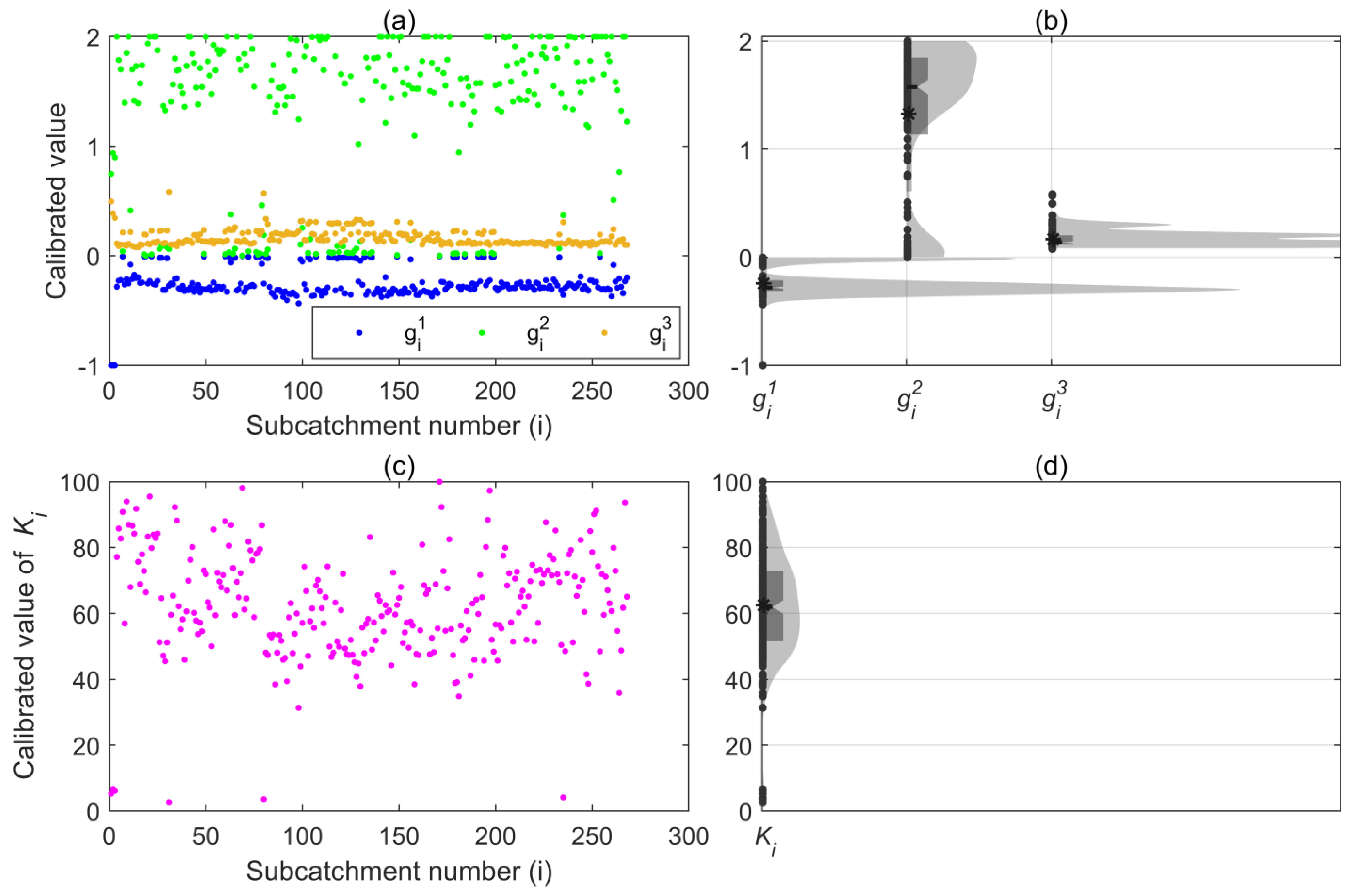
4.2. Performance of Distributed Time Variant Gain Model

Figure 3a shows the performance of the DTVGM-SWMM based on the NSE values of each subcatchment in the calibration phase (i.e., Chicago-1) and validation phase (i.e., Chicago-2 and Event-20170820). We can see that most subcatchments under the three storms have an NSE > 0.6, with only five exceptions: subcatchments 13, 31, 171, and 238 under Event-20170820. Figure 3b further illustrates these cases, displaying a positive correlation trend between the calibration and validation NSE values. For most subcatchments, especially the underperformed five subcathments, NSE values under Chicago-2 are greater than those under Event-20170820 because the former pattern is more similar to Chicago-1, which was used for calibration. Figure 3c presents the violin plot to analyze the statistical characteristics of the NSE values. We found that the average (median) NSE values for the runoff simulation under the three storm events were 0.92, 0.71, and 0.84 (0.91, 0.64, and 0.85), respectively, indicating an acceptable model performance. Overall, the DTVGM could simulate the runoff over 263 subcatchments (98.1% of all).
Figure 4 shows the calibrated parameters (g1, g2, g3, and K) of the DTVGM runoff module. The values of g1 and g3 for different subcatchments displayed more variance than the values of g2 (Figure 1a,b); the values of K had a considerable variation range (Figure 1c,d). In a subcatchment, the value of the four parameters reflected the complicated runoff generation characteristics in urban areas because g1 and g2 are gain parameters of surface runoff, and g3 is that of subsurface runoff. For example, in most subcatchments, a greater g1 value denotes a higher conversion from rainfall to runoff; for g2, a greater value denotes a greater impact of soil moisture on the surface runoff generation. However, to some extent, the four parameters were not entirely based on physical mechanisms, but were obtained using a statistical method. Further work should be conducted on the parameter explanation based on a detailed investigation of the hydrological conditions in each subcatchment.
Table 3 lists the statistics of the calibrated parameters of DTVGM for all subcatchments. We found that all the parameters’ values were within the range of variation, i.e., subjected to the constraints in Equation (7). Moreover, these calibrated parameters were consistent with other studies on DTVGM [10]. Overall, these results suggest that the calibration of DTVGM was reasonable.

4.3. Catchment Runoff and Outflow Simulations

The catchment runoff time series was calculated as the sum of the subcatchments’ runoff time series. For a subcatchment under a given storm event, two runoff time series were obtained by the SWMM simulation and the DTVGM-SWMM. Then, they were used to calculate the NSE with Equation (5), the relative error of runoff depth with Equation (8), and the relative error peak runoff with Equation (9). The calibrated DTVGM runoff module, determined based on the NSE values in Section 4.2, was used to generate the subcatchment runoff time series under different rainfalls. These series were finally used to drive the SWMM routing module to obtain the catchment outflow series.
We analyzed the applicability of DTVGM-SWMM by comparing the simulation results with those of SWMM in Figure 5, which illustrates the time series of rainfall, and the corresponding catchment runoff and outflow (simulated by DTVGM and SWMM) in calibration and validation phases. We found that the outflow time series were flattened after routing, and the times to peak were delayed. In addition, we found that the simulated hydrographs by DTVGM or DTVGM-SWMM demonstrated a good fit to those by SWMM under all storm events, especially in the rising and receding limbs.
However, there were gaps in the magnitudes of the peak runoffs of two simulations. Specifically, the DTVGM runoff module underestimated the peak runoff in the calibration phase of Chicago-1 (Figure 5a) and the validation phase of Event-20170909 (Figure 5d), but overestimated them in the validation phase of Chicago-2 and Event-20170820 (Figure 5b,c); similar phenomena were also found for the catchment outflow estimation by DTVGM-SWMM. No pattern of underestimation or overestimation was observed from these simulations. That is, the calibrated DTVGM demonstrated considerable uncertainty in predicting the peak rate of runoff. This can be explained by the fact that only the NSE, which reflects the accuracy and precision of the simulation for the entire time, was chosen as the objective function for calibrating the DTVGM runoff module. To conclude, the peak outflows of DTVGM-SWMM under three validation storms were very different from those of SWMM, one main reason being the poor simulation of peak runoff by DTVGM.

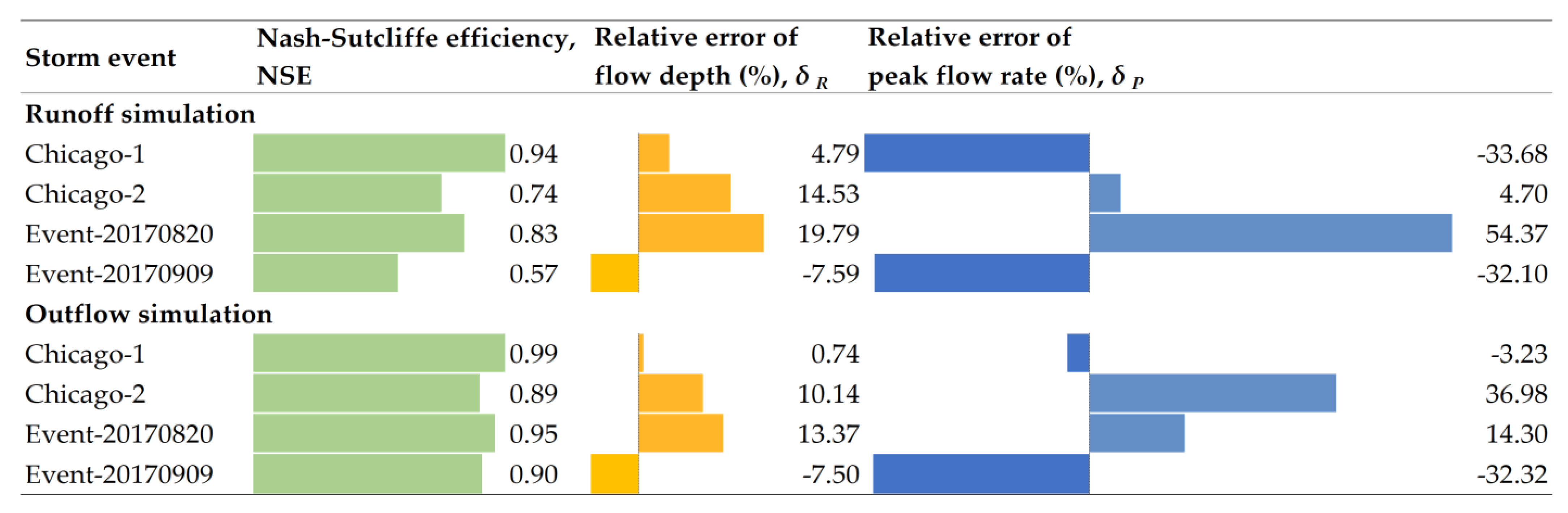
4.4. Performance of Coupling Model

Table 4 lists the statistics of the runoff and outflow time series simulated by SWMM and DTVGM-SWMM under different storms (illustrated in Figure 5). The depths and peak flow rates of runoffs and outflows were as given for the subsequent evaluation. We observed that the outflow depths might be greater than the runoff depths under a given storm for the SWMM model, but not for the DTVGM-SWMM model because SWMM considers the rainfall-derived inflow and infiltration into sewage infrastructure [41,42], while the coupling model neglects this.
Figure 6 summarizes the performance criteria of DTVGM-SWMM for estimating the runoff and outflow time series at a catchment scale under storm events (described in Table 1). We observed that:
First, the NSE values of the runoff and outflow simulations during the validation phase (Chicago-2, Event-20170820, and Event-20170909) were smaller than those for the calibration phase (Chicago-1), which is to be expected. The NSE minimum was 0.57 (runoff simulation under Event-20170909), suggesting a satisfactory accuracy for runoff and outflow simulations. In any case, for all storm events, the NSE value of the outflow simulation was higher than that of the runoff simulation. During the validation phase, the runoff simulation under Event-20170820 outperformed that under Chicago-2 and Event-20170909. The outflow simulation was similar. The NSE values of outflow simulation showed a strong correlation with the values of runoff simulation. In short, the NSE values indicate an acceptable performance for overall catchment runoff and outflow simulation.
Second, during validation, the absolute maxima of the relative error of flow depth (δR) were 19.79% for the runoff simulation and 13.37% for the outflow simulation; they were both under Event-20170820, which had the largest NSE values. We found that when the calibrated DTVGM-SWMM simulated runoff well in terms of overall fit, the runoff depth would be poorly estimated. A similar pattern could be found for the outflow simulation.
Third, δR values under Chicago-1, Chicago-2, and Event-20170820 were positive, indicating that estimations by DTVGM-SWMM were higher than those of SWMM; under Event-20170909, it was the opposite. For any storm event, the outflow depth simulation was better than the runoff depth simulation. Overall, the runoff and outflow depth simulations were reasonable and acceptable.
Fourth, the absolute maxima of the relative error of peak flow (δP) were 54.37% for runoff (under Event-20170820) and 36.98% for outflow (under Chicago-2). In most cases (7 out of 8), δ P was greater than δ R except in the runoff simulation under Chicago-2 (i.e., δP = 4.70, δR = 14.53).
Overall, the DTVGM-SWMM had a sizable relative error in runoff depth but a small relative error in the outflow depth after the routing process. The reason is that only the NSE was considered in the objective function for the model calibration without considering the accuracy of simulating the peak runoff where the duration is short. The DTVGM runoff module was well-calibrated for estimating the runoff process at the catchment scale, and the DTVGM-SWMM showed high accuracy in outflow simulation.

5. Conclusions

We proposed and validated the DTVGM-SWMM by combining the DTVGM runoff module with the SWMM routing module to develop a simple and efficient model for rainfall-runoff simulation in a sponge city. We conclude that: (1) the NSE and relative error of flow depth are good when using the calibrated coupling model to simulate the catchment runoff and outflow processes, especially for estimating outflows; (2) the relative errors of peak flow rate were significant for runoff and outflow simulation, indicating that the calibrated DTVGM-SWMM is bad in predicting peak flow rates for urban catchment. Overall, the proposed model can characterize the nonlinear characteristics of rainfall-runoff with few parameters; thus, it can be used for effective and efficient prediction, like machine learning models.
This research demonstrates that the DTVGM-SWMM excels in simulating catchment runoff and outflows in a sponge city. Future studies can be conducted on: (1) packaging the DTVGM-SWMM into software, like Mat-SWMM [14], and developing a feature that models the runoff for different underlying surfaces and the LIDs constructed in sponge cities; (2) improving the calibration by taking the peak flow rate as another objective function, as well as using more performance indicators; (3) investigating and quantifying the uncertainty (input data, structure, and parameters of the DTVGM and SWMM used), sensitivity, efficiency, and ease of development, and comparing them with other distributed models; and (4) developing and integrating a multi-objective decision-making tool for LIDs implementation [43,44].

Author Contributions

Conceptualization, Y.Y.; methodology, Y.Y.; software, Z.L.; validation, W.Z.; formal analysis, Z.L.; investigation, W.Z.; resources, J.X. and Q.H.; data curation, W.Z.; writing—original draft preparation, Y.Y.; writing—review and editing, Y.Y. and D.L.; visualization, W.Z. and D.L.; supervision, Q.H.; project administration, Y.Y.; funding acquisition, Y.Y. All authors have read and agreed to the published version of the manuscript.

Funding

This research was funded by the National Natural Science Foundation of China, grant numbers 52009099 and 52279025. The APC was funded by the China Postdoctoral Science Foundation Funded Project, grant number 2019M653882XB.

Institutional Review Board Statement

Not applicable.

Informed Consent Statement

Not applicable.

Data Availability Statement

Not applicable.

Acknowledgments

The authors acknowledge the Fengxi Management Committee for its assistance. We thank the editors and reviewers for their helpful comments and suggestions.

Conflicts of Interest

The authors declare no conflict of interest.

References

  1. Yang, Y. Study on Ideal Way of Water Environment Improvement by China’s Sponge City Construction. Doctoral Thesis, Nihon University, Tokyo, Japan, 2017. [Google Scholar]
  2. Thu Thuy, N.; Huu Hao, N.; Guo, W.; Wang, X.C.; Ren, N.; Li, G.; Ding, J.; Liang, H. Implementation of a specific urban water management—Sponge City. Sci. Total Environ. 2019, 652, 147–162. [Google Scholar] [CrossRef]
  3. Fang, C.; Cui, X.; Li, G.; Bao, C.; Wang, Z.; Ma, H.; Sun, S.; Liu, H.; Luo, K.; Ren, Y. Modeling regional sustainable development scenarios using the Urbanization and Eco-environment Coupler: Case study of Beijing Tianjin-Hebei urban agglomeration, China. Sci. Total Environ. 2019, 689, 820–830. [Google Scholar] [CrossRef] [PubMed]
  4. Hou, J.; Mao, H.; Li, J.; Sun, S. Spatial simulation of the ecological processes of stormwater for sponge cities. J. Environ. Manag. 2019, 232, 574–583. [Google Scholar] [CrossRef] [PubMed]
  5. Gong, Y.; Yin, D.; Fang, X.; Li, J. Factors Affecting Runoff Retention Performance of Extensive Green Roofs. Water 2018, 10, 1217. [Google Scholar] [CrossRef] [Green Version]
  6. Zakizadeh, F.; Moghaddam Nia, A.; Salajegheh, A.; Sanudo-Fontaneda, L.A.; Alamdari, N. Efficient Urban Runoff Quantity and Quality Modelling Using SWMM Model and Field Data in an Urban Watershed of Tehran Metropolis. Sustainability 2022, 14, 1086. [Google Scholar] [CrossRef]
  7. Rossman, L.A. SWMM-CAT User’s Guide. 2014. Available online: http://nepis.epa.gov/Adobe/PDF/P100KY8L.PDF (accessed on 16 January 2023).
  8. Palla, A.; Gnecco, I. Hydrologic modeling of Low Impact Development systems at the urban catchment scale. J. Hydrol. 2015, 528, 361–368. [Google Scholar] [CrossRef]
  9. Song, Z.H.; Xia, J.; Wang, G.S.; She, D.X.; Hu, C.; Hong, S. Regionalization of hydrological model parameters using gradient boosting machine. Hydrol. Earth Syst. Sci. 2022, 26, 505–524. [Google Scholar] [CrossRef]
  10. Hu, C.; Xia, J.; She, D.; Song, Z.; Zhang, Y.; Hong, S. A new urban hydrological model considering various land covers for flood simulation. J. Hydrol. 2021, 603, 126833. [Google Scholar] [CrossRef]
  11. Liu, Z. Coupled Study of Distributed Time Variant Gain Model and Storm Water Management Model. Master’s Thesis, Xi’an University of Technology, Xi’an, China, 2022. [Google Scholar]
  12. Yang, Y.; Li, J.; Huang, Q.; Xia, J.; Li, J.; Liu, D.; Tan, Q. Performance assessment of sponge city infrastructure on stormwater outflows using isochrone and SWMM models. J. Hydrol. 2021, 597, 126151. [Google Scholar] [CrossRef]
  13. Liu, D.; Huang, Q.; Yang, Y.Y.; Liu, D.F.; Wei, X.T. Bi-objective algorithm based on NSGA-II framework to optimize reservoirs operation. J. Hydrol. 2020, 585, 124830. [Google Scholar] [CrossRef]
  14. Riaño-Briceño, G.; Barreiro-Gomez, J.; Ramirez-Jaime, A.; Quijano, N.; Ocampo-Martinez, C. MatSWMM—An open-source toolbox for designing real-time control of urban drainage systems. Environ. Model. Softw. 2016, 83, 143–154. [Google Scholar] [CrossRef] [Green Version]
  15. Hou, J.; Li, D.; Wang, X.; Guo, K.; Tong, y.; Ma, Y. Simulation of the effect of pre-conditioning of LID measures on runoff regulation at the building plot scale. Adv. Water Sci. 2019, 30, 45–55. [Google Scholar] [CrossRef]
  16. Bai, T.; Mayer, A.L.; Shuster, W.D.; Tian, G. The Hydrologic Role of Urban Green Space in Mitigating Flooding (Luohe, China). Sustainability 2018, 10, 3584. [Google Scholar] [CrossRef] [PubMed] [Green Version]
  17. Dai, Y.; Jiang, J.; Gu, X.; Zhao, Y.; Ni, F. Sustainable Urban Street Comprising Permeable Pavement and Bioretention Facilities: A Practice. Sustainability 2020, 12, 8288. [Google Scholar] [CrossRef]
  18. Li, W.; Wang, H.; Zhou, J.; Yan, L.; Liu, Z.; Pang, Y.; Zhang, H.; Huang, T. Simulation and Evaluation of Rainwater Runoff Control, Collection, and Utilization for Sponge City Reconstruction in an Urban Residential Community. Sustainability 2022, 14, 12372. [Google Scholar] [CrossRef]
  19. Zhang, C.; Wang, Y.; Li, Y.; Ding, W. Vulnerability Analysis of Urban Drainage Systems: Tree vs. Loop Networks. Sustainability 2017, 9, 397. [Google Scholar] [CrossRef] [Green Version]
  20. Goncalves, M.L.R.; Zischg, J.; Rau, S.; Sitzmann, M.; Rauch, W.; Kleidorfer, M. Modeling the Effects of Introducing Low Impact Development in a Tropical City: A Case Study from Joinville, Brazil. Sustainability 2018, 10, 728. [Google Scholar] [CrossRef] [Green Version]
  21. Mora-Melia, D.; Lopez-Aburto, C.S.; Ballesteros-Perez, P.; Munoz-Velasco, P. Viability of Green Roofs as a Flood Mitigation Element in the Central Region of Chile. Sustainability 2018, 10, 1130. [Google Scholar] [CrossRef] [Green Version]
  22. Lee, S.; Kang, T.; Sun, D.; Park, J.-J. Enhancing an Analysis Method of Compound Flooding in Coastal Areas by Linking Flow Simulation Models of Coasts and Watershed. Sustainability 2020, 12, 6572. [Google Scholar] [CrossRef]
  23. Barbaro, G.; Miguez, M.G.; de Sousa, M.M.; Ribeiro da Cruz Franco, A.B.; Canedo de Magalhaes, P.M.; Foti, G.; Valadao, M.R.; Occhiuto, I. Innovations in Best Practices: Approaches to Managing Urban Areas and Reducing Flood Risk in Reggio Calabria (Italy). Sustainability 2021, 13, 3463. [Google Scholar] [CrossRef]
  24. de Farias Mesquita, J.B.; Lima Neto, I.E. Coupling Hydrological and Hydrodynamic Models for Assessing the Impact of Water Pollution on Lake Evaporation. Sustainability 2022, 14, 13465. [Google Scholar] [CrossRef]
  25. Lee, J.M.; Park, M.; Min, J.-H.; Kim, J.; Lee, J.; Jang, H.; Na, E.H. Evaluation of SWMM-LID Modeling Applicability Considering Regional Characteristics for Optimal Management of Non-Point Pollutant Sources. Sustainability 2022, 14, 14662. [Google Scholar] [CrossRef]
  26. Liu, B.; Xu, C.; Yang, J.; Lin, S.; Wang, X. Effect of Land Use and Drainage System Changes on Urban Flood Spatial Distribution in Handan City: A Case Study. Sustainability 2022, 14, 14610. [Google Scholar] [CrossRef]
  27. Quichimbo-Miguitama, F.; Matamoros, D.; Jimenez, L.; Quichimbo-Miguitama, P. Influence of Low-Impact Development in Flood Control: A Case Study of the Febres Cordero Stormwater System of Guayaquil (Ecuador). Sustainability 2022, 14, 7109. [Google Scholar] [CrossRef]
  28. Yang, Y.; Li, Y.; Huang, Q.; Xia, J.; Li, J. Surrogate-based multiobjective optimization to rapidly size low impact development practices for outflow capture. J. Hydrol. 2023, 616, 128848. [Google Scholar] [CrossRef]
  29. Rossman, L.A. Storm Water Management Model Reference Manual (Volume I—Hydrology). 2016. Available online: http://nepis.epa.gov/Exe/ZyPDF.cgi?Dockey=P100NYRA.txt (accessed on 16 January 2023).
  30. Rossman, L.A. Storm Water Management Model User’s Manual, Version 5.1 ed. 2015. Available online: https://www.epa.gov/water-research/storm-water-management-model-swmm-version-51-users-manual (accessed on 16 January 2023).
  31. Li, X.; Wei, Y.; Li, F. Optimality of antecedent precipitation index and its application. J. Hydrol. 2021, 595, 126027. [Google Scholar] [CrossRef]
  32. Rasheed, Z.; Aravamudan, A.; Gorji Sefidmazgi, A.; Anagnostopoulos, G.C.; Nikolopoulos, E.I. Advancing flood warning procedures in ungauged basins with machine learning. J. Hydrol. 2022, 609, 127736. [Google Scholar] [CrossRef]
  33. Fedora, M.A.; Beschta, R.L. Storm runoff simulation using an antecedent precipitation index (API) model. J. Hydrol. 1989, 112, 121–133. [Google Scholar] [CrossRef]
  34. Xu, S.; Chen, Y.; Zhang, Y.; Chen, L.; Sun, H.; Liu, J. Developing a Framework for Urban Flood Modeling in Data-poor Regions. J. Hydrol. 2022, 617, 128985. [Google Scholar] [CrossRef]
  35. Wang, W.; Liu, J.; Xu, B.; Li, C.; Liu, Y.; Yu, F. A WRF/WRF-Hydro coupling system with an improved structure for rainfall-runoff simulation with mixed runoff generation mechanism. J. Hydrol. 2022, 612, 128049. [Google Scholar] [CrossRef]
  36. Luan, G.; Hou, J.; Yang, L.; Wang, T.; Pan, Z.; Li, D.; Gao, X.; Fan, C. A High-resolution Comprehensive Water Quality Model Based on GPU Acceleration Techniques. J. Hydrol. 2022, 617, 128814. [Google Scholar] [CrossRef]
  37. Ichiba, A.; Gires, A.; Tchiguirinskaia, I.; Schertzer, D.; Bompard, P.; Ten Veldhuis, M.C. Scale effect challenges in urban hydrology highlighted with a distributed hydrological model. Hydrol. Earth Syst. Sci. 2018, 22, 331–350. [Google Scholar] [CrossRef] [Green Version]
  38. Avellaneda, P.M.; Jefferson, A.J.; Grieser, J.M.; Bush, S.A. Simulation of the cumulative hydrological response to green infrastructure. Water Resour. Res. 2017, 53, 3087–3101. [Google Scholar] [CrossRef]
  39. Brunetti, G.; Šimůnek, J.; Piro, P. A comprehensive numerical analysis of the hydraulic behavior of a permeable pavement. J. Hydrol. 2016, 540, 1146–1161. [Google Scholar] [CrossRef] [Green Version]
  40. Li, Y.; Mo, S.; Yang, Y.; Liu, D. Optimization of the proportion of LID facilities deployment in sponge cities based on NSGA-II algorithm. Water Wastewater Eng. 2021, 57, 475–481. [Google Scholar] [CrossRef]
  41. Diem, J.E.; Pangle, L.A.; Milligan, R.A.; Adams, E.A. How much water is stolen by sewers? Estimating watershed-level inflow and infiltration throughout a metropolitan area. J. Hydrol. 2022, 614, 128629. [Google Scholar] [CrossRef]
  42. Zhang, K.; Parolari, A.J. Impact of stormwater infiltration on rainfall-derived inflow and infiltration: A physically based surface–subsurface urban hydrologic model. J. Hydrol. 2022, 610, 127938. [Google Scholar] [CrossRef]
  43. Xie, M.; Cheng, Y.; Dong, Z. Study on Multi-Objective Optimization of Sponge Facilities Combination at Urban Block Level: A Residential Complex Case Study in Nanjing, China. Water 2022, 14, 3292. [Google Scholar] [CrossRef]
  44. Hassani, M.R.; Niksokhan, M.H.; Janbehsarayi, S.F.M.; Nikoo, M.R. Multi-objective robust decision-making for LIDs implementation under climatic change. J. Hydrol. 2023, 617, 128954. [Google Scholar] [CrossRef]
Figure 1. Map of the study site. (a) Location of Shannxi Province, China. (b) Fengxi sponge city pilot region, the study site for simulations. (c) Subcatchment divisions and generalized drainage system in the storm water management model with 210 green roofs, 257 porous pavements, and 268 bioretention cells. (d) Stormwater-related facilities. (Sources: Yang et al. [12]).
Sustainability 15 03804 g001
Figure 2. Framework of coupling DTVGM and SWMM. DTVGM, distributed time variant gain model; SWMM, storm water management model; DTVGM-SWMM, the runoff module of DTVGM with the routing module of SWMM; GA, genetic algorithm.
Sustainability 15 03804 g002
Figure 3. Nash–Sutcliffe efficiency (NSE) values by subcatchment of DTVGM-SWMM under three storm events. Note that the NSE value of a subcatchment in the graph is the largest one obtained from 30 iterations of DTVGM calibration, that is, the biggest NSE value during calibration. (a) NSE values of 268 subcatchments. (b) Five subcatchments that have NSE < 0.6. (c) Violin plot of NSE ranges by storm event. The markers * and—denote the mean value and median, respectively.
Sustainability 15 03804 g003
Figure 4. Calibrated parameters of distributed time variant gain model by subcatchment. (a) Values and (b) statistics of g i 1 , g i 2 , and g i 3 . (c) Values and (d) statistics of K i . The markers * and—denote the mean value and median, respectively.
Sustainability 15 03804 g004
Figure 5. Hyetograph of storm events for calibration and validation; hydrographs of catchment runoff and outflow simulated by storm water management model and the coupling model.
Sustainability 15 03804 g005
Figure 6. Performance indicators of goodness-of-fit for catchment runoff and outflow simulation using DTVGM-SWMM. Chicago-1 was used for calibrating, and the other storms were used for validation.
Sustainability 15 03804 g006
Table 1. Statistics of storm events used to calibrate and validate the SWMM and DTVGM-SWMM.
Storm
Event
Name
Return
Period
(Year)
Duration
(min)
Time-to-Peak
Coefficient
Depth (mm)Mean
Intensity
(mm/min)
Usage
Chicago-1 111200.3520.670.17Calibrate DTVGM-SWMM
Chicago-221200.3527.920.23Validate DTVGM-SWMM
Event-20170820 2n/a960.5713.400.14Calibrate SWMM and Validate DTVGM-SWMM
Event-20170909n/a9680.4716.000.02Calibrate SWMM and Validate DTVGM-SWMM
Event-20170916n/a7710.3611.400.01Calibrate SWMM
1 For simplicity, Chicago denotes a rainfall time series calculated using Equation (1) of Yang et al. [12]. 2 Event denotes a rainfall time series and the corresponding outflows recorded at that time.
Table 3. Statistics of calibrated parameters of distributed time variant gain model for all subcatchments.
VariableRange of VariationCalibrated Value
AverageMedianMinimumMaximum
g1[−1, 1]−0.241−0.281−1.000−0.004
g2[0, 2]1.3261.5750.0002.000
g3[0, 1]0.1690.1380.0780.583
K[0, 100]62.46961.9062.619100.000
Table 4. Depths and peak flow rates of runoff and outflow simulated by storm water management model and the coupling model under four storm events.
StormChicago-1Chicago-2Event-20170820Event-20170909
Precipitation (mm)20.6727.9213.4016.00
SWMM model
Runoff depth (mm)2.414.071.062.75
Outflow depth (mm)2.454.121.082.65
Peak runoff rate (m3/s)10.9023.541.998.72
Peak outflow rate (m3/s)3.627.760.983.72
DTVGM-SWMM model
Runoff depth (mm)2.534.671.272.54
Outflow depth (mm)2.474.531.222.45
Peak runoff rate (m3/s)7.2324.653.075.92
Peak outflow rate (m3/s)3.5010.631.122.52
Disclaimer/Publisher’s Note: The statements, opinions and data contained in all publications are solely those of the individual author(s) and contributor(s) and not of MDPI and/or the editor(s). MDPI and/or the editor(s) disclaim responsibility for any injury to people or property resulting from any ideas, methods, instructions or products referred to in the content.

