


Parameter Extraction of Solar Photovoltaic Cell and Module Models with Metaheuristic Algorithms: A Review

Abstract
:1. Introduction
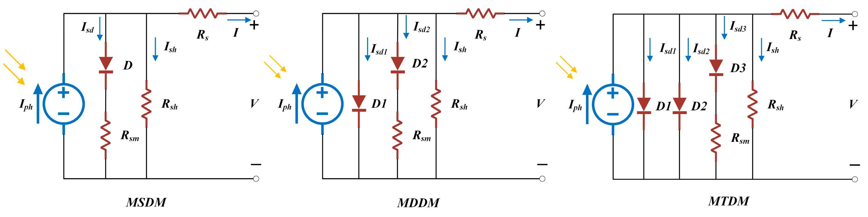
- The mathematical models of current commonly used SDM, DDM, TDM, and PV modules are explained;
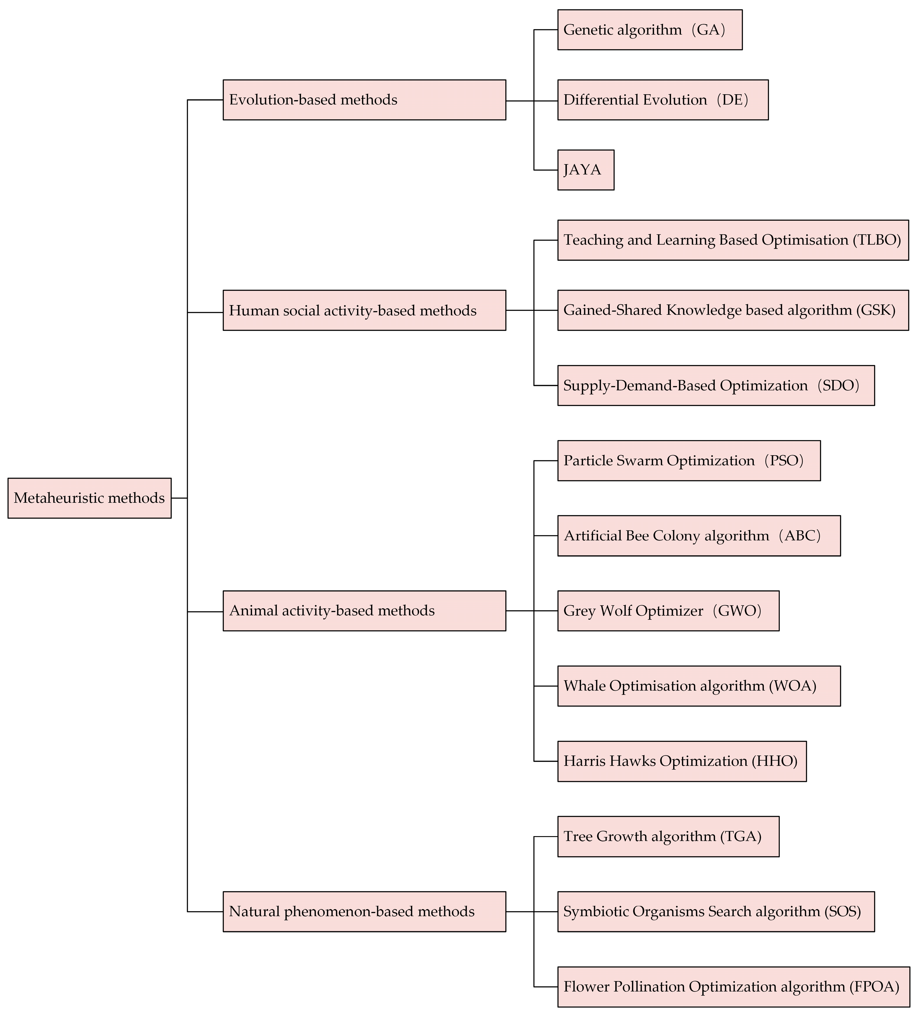
- The characteristics of each metaheuristic method and their enhancements and applications are outlined;
- The statistical results of RMSE, TNFES, SIAE and algorithmic settings of selected metaheuristics are summarized and compared;
- The output characteristics of the PV system are discussed for the dynamic temperature, irradiance, and partial shading, and the variation in parameters and RMSE are analyzed;
- Existing challenges and possible future work focuses are analyzed and provided.
2. PV Models and Problem Formulations
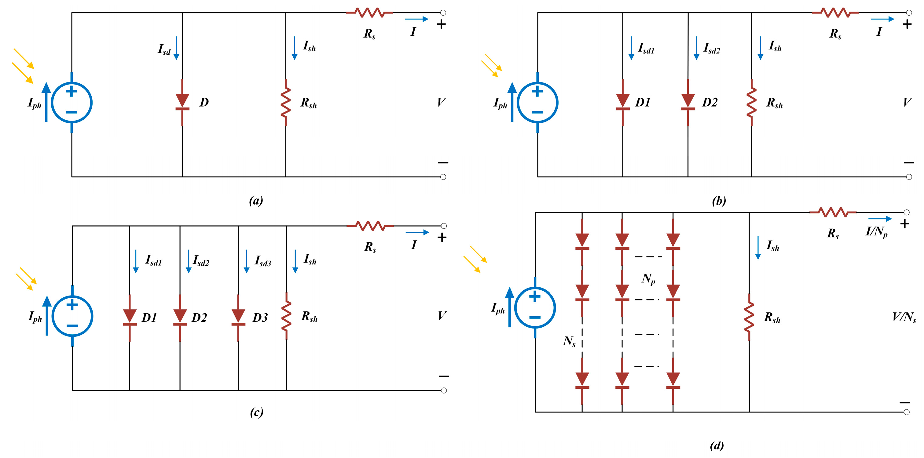
2.1. PV Models
2.1.1. SDM
2.1.2. DDM
2.1.3. TDM
2.1.4. PV Module
2.1.5. PV Model Review
2.2. Problem Formulations
2.3. Indicators Summary
- Friedman test (FT), Wilcoxon rank sum test (WRT), and Wilcoxon signed rank test (WST): they broaden evaluation scales from statistical perspectives;
- In addition, a few works in the literature also use evaluation indicators such as the sum of squares of power, current, and voltage errors (ERR) [61].
3. Methods and Results
3.1. GAs
3.2. DEs
3.3. PSOs
3.4. ABCs
3.5. GWOs
3.6. JAYAs
3.7. TLBOs
3.8. WOAs
3.9. Hybrids
3.10. Others
4. Whole Analysis and Research Prospects
4.1. Data Analysis
- The STD of RMSE reflects the results’ robustness, MIN RMSE means the results’ accuracy, and other RMSEs denote the range and sharpness of the fluctuations in the results. The SDM, DDM and Photowatt-PWP201 models of DEDIWPSO had the MIN RMSE (7.730062 × 10⁻⁴, 7.182306 × 10⁻⁴, and 2.03992 × 10⁻³), mean RMSE (7.730062 × 10⁻⁴, 7.187462 × 10⁻⁴, and 2.03992 × 10⁻³), MAX RMSE (7.730062 × 10⁻⁴, 7.3181 × 10⁻⁴, and 2.03992 × 10⁻³) and STD (5.18668 × 10⁻¹⁵, 2.486129 × 10⁻⁶, and 2.995389 × 10⁻¹⁵). It is followed by IGSK with MIN RMSE (9.8602188 × 10⁻⁴, 9.8248485 × 10⁻⁴, and 2.4250749 × 10⁻³), mean RMSE (9.8602188 × 10⁻⁴, 9.8272774 × 10⁻⁴, and 2.4250749 × 10⁻³), MAX MRSE (9.8602188 × 10⁻⁴, 9.8602188 × 10⁻⁴, and 2.4250749 × 10⁻³) and STD (3.5821018 × 10⁻¹⁷, 8.9578942 × 10⁻⁷, and 2.9226647 × 10⁻¹⁷). Then, EOTLBO, OLBGWO, CSOOJAYA, RLDE, ABC-TRR, IWOA, TLBOBSA, HSOA, and SOS followed.
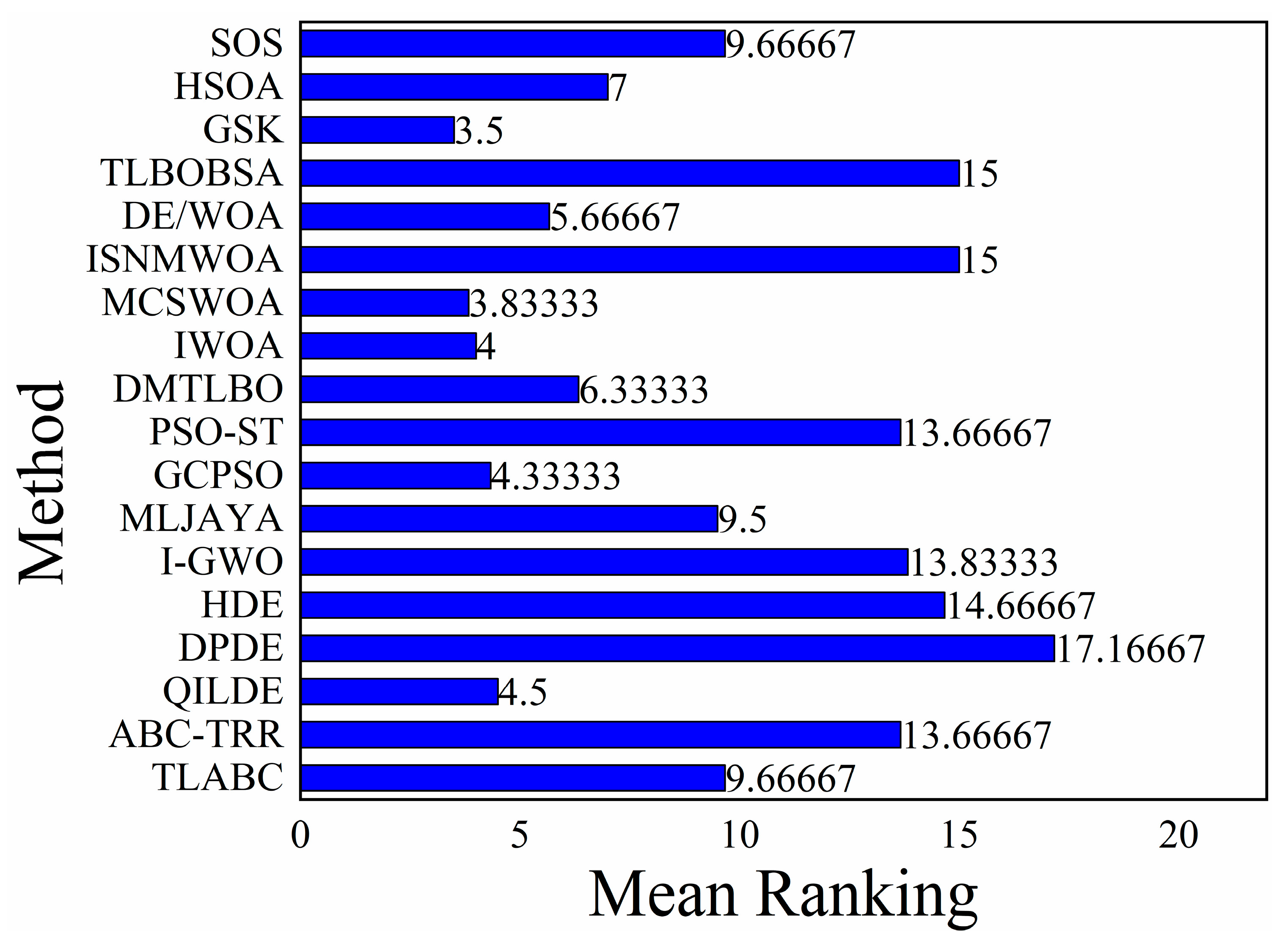
- Figure 4 shows the combined FT ranking for the SDM, DDM, and Photowatt-PWP201. It combines the absolute accuracy of the methods in a wide range of cases. GSK ranks first, followed by MCSWOA, IWOA, GCPSO, QILDE, DE/WOA, DMTLBO, HSOA, MLJAYA, SOS, TLABC, PSO-ST, ABC-TRR, I-GWO, HDE, TLBOBSA, ISNMWOA, and DPDE. GSK, as a new method achieving the highest accuracy, demonstrates the need to explore the performance of new schemes in this issue. It is worth noting that the rankings of the same methods in different PV models may differ, which indicates that different PV models have varied preferences for algorithms.
- TNFES is related to the computational resources consumed, with a lower TNFES representing a lower computational burden. For the SDM and module, ABC-TRR had the fewest TNFES (1000) while other methods basically used a TNFES of 50,000. For the DDM, ABC-TRR had the fewest TNFES (5000), while most of the rest consumed a TNFES of 50,000.
4.2. Analysis of Temperature and Irradiance Influences
4.2.1. Uniform Irradiance and Temperature
4.2.2. Partial Shade Conditions
4.3. Analysis of Modified Diode Models’ Works
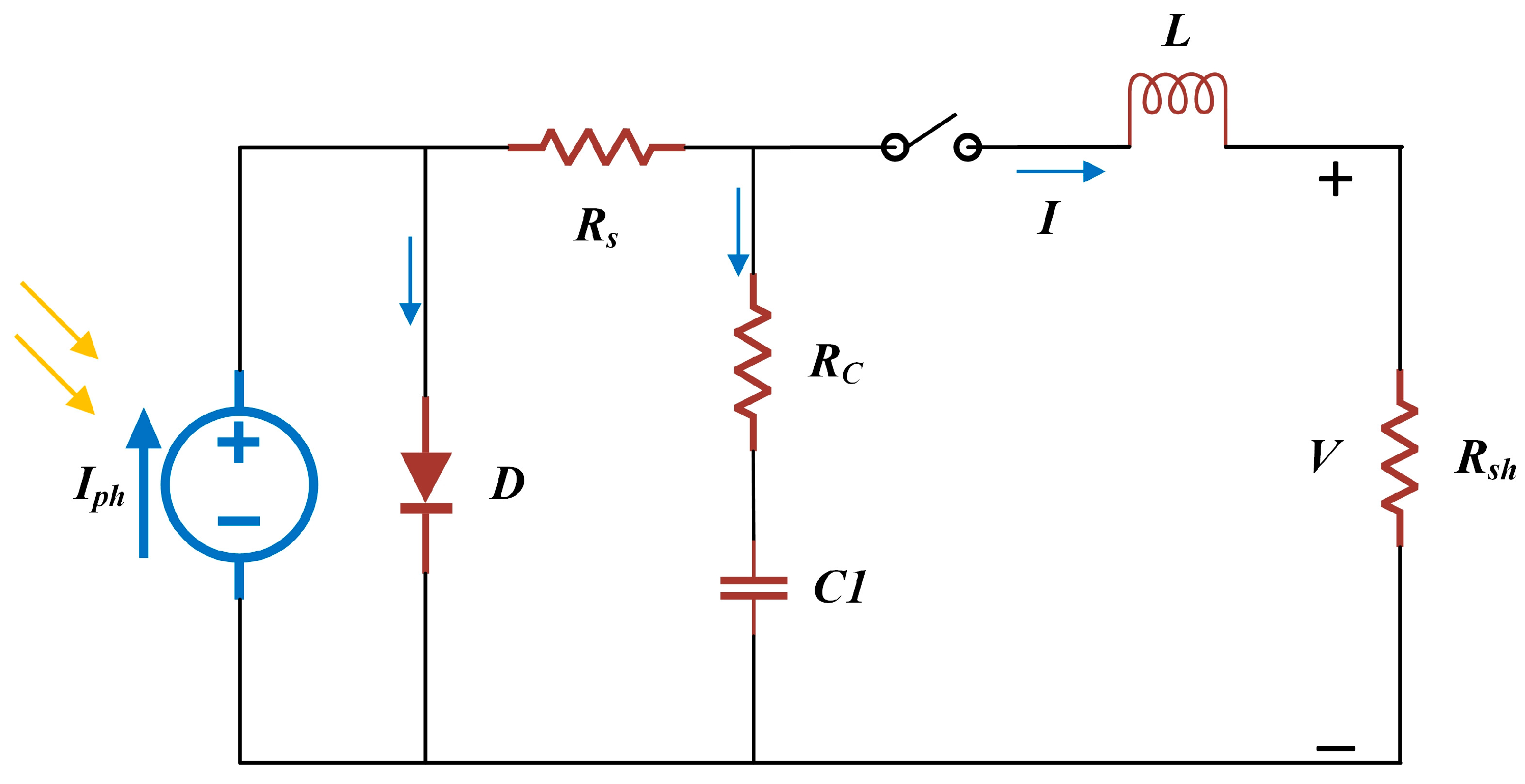
4.4. Analysis of Dynamic Models’ Works
4.5. Whole Analysis
- The promotion of GA has been rare in recent years, and accuracy is supposed to be enhanced.
- DE’s convergence rate and PSO’s accuracy could improve.
- ABC is weakly exploited and significant in parameter settings.
- GWO and WOA have few parameters and struggle with multi-dimensional issues.
- JAYA and TLBO’s promotions are flawed in accuracy.
- Hybrid approaches may complicate the implementation and introduce additional parameters.
- New approaches are not sufficiently balanced for specific issues. For example, GSK, SDO, TGA, and SOS are under-exploited, and HHO and FPOA are under-explored.
- TNFES is a sign of computational resources, yet its value is almost pitched at 50,000. Reducing TNFES without compromising accuracy is imperative.
- More diodes in the cell model may increase the extraction accuracy. Recently, a four diode model was proposed [47] and the results showed good fitting effect. However, more diodes also indicate more parameters that need to be extracted and solutions are also more intractable. Hence, selecting a suitable PV model for an algorithm is challenging.
- Some of the literature used too few PV cases to demonstrate metaheuristics’ generalizability.
- Metaheuristics’ effectiveness is devoid of practical engineering applications.
- More and exact measured data means more accurate extraction results, but obtaining sufficient high-precision measurements is challenging and costly.
- In engineering, running time is pivotal. Hence, cutting running times is a challenge.
- Multiple matrices are imperative to signal the competitiveness of metaheuristic results, yet some of the literature adopted few matrices for comparison.
4.6. Research Prospects
- Exploration techniques such as chaotic mapping and second-order oscillation mechanisms can be considered to incorporate into GA. They are envisaged to augment accuracy and robustness.
- DE might be combined with exploitation-based metaheuristics, such as the Search Backtracking Algorithm, or with search mechanisms that accelerate the convergence. PSO demands more diversity-raising search mechanisms such as trust region reflection, taboo search, and fitness distance balance. Additionally, studies on adapting their parameters are well-tried.
- ABC considers introducing neighborhood search and adaptive mechanisms to speed up the convergence.
- For GWO and WOA, adaptive operators could be inserted to improve applicability in the face of high-dimensional issues.
- JAYA and TLBO could borrow the exploration-type mechanisms in CSOOJAYA, MTLBO, and EBLSHADE to improve the overall performance.
- Hybrid methods can identify contributing components through component analysis and remove unimportant components to alleviate implementation redundancy.
- New methods can adopt adaptive learning, neighborhood search, chaotic mapping, and algorithmic blending techniques to enhance their behavior.
- For the parameter extraction, diminishing computational resources’ consumption is at stake. Reducing TNFES while maintaining the same accuracy by introducing different techniques, i.e., local search and reinforcement learning, is a direction worthy of further research.
- Some methods are feasible for low-dimensional issues, and some deliver better performance for high-dimensional issues. Meanwhile, the selection of MSDM, MDDM, MTDM, and FDM with 6, 8, 10, and 11 unknown parameters to be included in the cell model is a future research direction for further performance improvement. Hence, it would be interesting to pick the right algorithm improvement to render PV models with desirable accuracy.
- For the issue of too few employed cases, more cases are considered in future research to reveal the methods’ generalizability. Examples include cases at different temperatures and irradiances and cases in partial shade.
- The real-time extraction of PV models’ parameters at different operating conditions is highly suggested. It is excellent work to accurately model the dynamics of photovoltaics for practical engineering problems.
- Faced with the problem of little measured data, inserting deep learning techniques such as neural networks to eliminate erroneous data and expand the amount of data for metaheuristic methods is an effective way to facilitate the extraction accuracy.
- The graphical processing unit (GPU) allows different solutions to be updated simultaneously to raise the efficiency. Thus, metaheuristic methods’ speed improvements can be geared toward direct runtime reductions through GPU-like devices.
- More performance evaluation indicators can demonstrate metaheuristic methods’ overall effectiveness more comprehensively. Therefore, introducing more multifaceted indicators is necessary to enhance persuasiveness.
5. Conclusions
Author Contributions
Funding
Institutional Review Board Statement
Informed Consent Statement
Data Availability Statement
Conflicts of Interest
References
- Li, Y.; Chiu, Y.H.; Lin, T.Y. Research on New and Traditional Energy Sources in OECD Countries. Int. J. Environ. Res. Public Health 2019, 16, 1122. [Google Scholar] [CrossRef]
- Ridha, H.M.; Heidari, A.A.; Wang, M.; Chen, H. Boosted mutation-based Harris hawks optimizer for parameters identification of single-diode solar cell models. Energy Convers. Manag. 2020, 209, 112660. [Google Scholar] [CrossRef]
- You, V.; Kakinaka, M. Modern and traditional renewable energy sources and CO(2) emissions in emerging countries. Environ. Sci. Pollut. Res. 2022, 29, 17695–17708. [Google Scholar] [CrossRef] [PubMed]
- Xiong, G.; Li, L.; Mohamed, A.W.; Yuan, X.; Zhang, J. A new method for parameter extraction of solar photovoltaic models using gaining–sharing knowledge based algorithm. Energy Rep. 2021, 7, 3286–3301. [Google Scholar] [CrossRef]
- Lin, S.; Zhang, C.; Ding, L.; Zhang, J.; Liu, X.; Chen, G.; Wang, S.; Chai, J. Accurate Recognition of Building Rooftops and Assessment of Long-Term Carbon Emission Reduction from Rooftop Solar Photovoltaic Systems Fusing GF-2 and Multi-Source Data. Remote Sens. 2022, 14, 3144. [Google Scholar] [CrossRef]
- Dixit, S. Solar technologies and their implementations: A review. Mater. Today Proc. 2020, 28, 2137–2148. [Google Scholar] [CrossRef]
- Kant Bhatia, S.; Palai, A.K.; Kumar, A.; Kant Bhatia, R.; Kumar Patel, A.; Kumar Thakur, V.; Yang, Y.H. Trends in renewable energy production employing biomass-based biochar. Bioresour. Technol. 2021, 340, 125644. [Google Scholar] [CrossRef]
- Qazi, A.; Hussain, F.; Rahim, N.A.B.D.; Hardaker, G.; Alghazzawi, D.; Shaban, K.; Haruna, K. Towards Sustainable Energy: A Systematic Review of Renewable Energy Sources, Technologies, and Public Opinions. IEEE Access 2019, 7, 63837–63851. [Google Scholar] [CrossRef]
- Rojas, D.; Rivera, M.; Wheeler, P. Basic Principles of Solar Energy. In Proceedings of the 2021 IEEE CHILEAN Conference on Electrical, Electronics Engineering, Information and Communication Technologies (CHILECON), Valparaíso, Chile, 6–9 December 2021; pp. 1–6. [Google Scholar]
- Saidur, R.; BoroumandJazi, G.; Mekhlif, S.; Jameel, M. Exergy analysis of solar energy applications. Renew. Sustain. Energy Rev. 2012, 16, 350–356. [Google Scholar] [CrossRef]
- Zheng, Y.; Weng, Q. Modeling the Effect of Green Roof Systems and Photovoltaic Panels for Building Energy Savings to Mitigate Climate Change. Remote Sens. 2020, 12, 2402. [Google Scholar] [CrossRef]
- Chen, D.-Y.; Peng, L.; Zhang, W.-Y.; Wang, Y.-D.; Yang, L.-N. Research on Self-Supervised Building Information Extraction with High-Resolution Remote Sensing Images for Photovoltaic Potential Evaluation. Remote Sens. 2022, 14, 5350. [Google Scholar] [CrossRef]
- Humada, A.M.; Darweesh, S.Y.; Mohammed, K.G.; Kamil, M.; Mohammed, S.F.; Kasim, N.K.; Tahseen, T.A.; Awad, O.I.; Mekhilef, S. Modeling of PV system and parameter extraction based on experimental data: Review and investigation. Sol. Energy 2020, 199, 742–760. [Google Scholar] [CrossRef]
- Kumari, P.A.; Geethanjali, P. Parameter estimation for photovoltaic system under normal and partial shading conditions: A survey. Renew. Sustain. Energy Rev. 2018, 84, 1–11. [Google Scholar] [CrossRef]
- Pillai, D.S.; Rajasekar, N. Metaheuristic algorithms for PV parameter identification: A comprehensive review with an application to threshold setting for fault detection in PV systems. Renew. Sustain. Energy Rev. 2018, 82, 3503–3525. [Google Scholar] [CrossRef]
- Humada, A.M.; Hojabri, M.; Mekhilef, S.; Hamada, H.M. Solar cell parameters extraction based on single and double-diode models: A review. Renew. Sustain. Energy Rev. 2016, 56, 494–509. [Google Scholar] [CrossRef]
- Selem, S.I.; El-Fergany, A.A.; Hasanien, H.M. Artificial electric field algorithm to extract nine parameters of triple-diode photovoltaic model. Int. J. Energy Res. 2020, 45, 590–604. [Google Scholar] [CrossRef]
- Xiong, G.; Zhang, J.; Shi, D.; Zhu, L.; Yuan, X.; Yao, G. Modified Search Strategies Assisted Crossover Whale Optimization Algorithm with Selection Operator for Parameter Extraction of Solar Photovoltaic Models. Remote Sens. 2019, 11, 2795. [Google Scholar] [CrossRef]
- Abbassi, R.; Abbassi, A.; Jemli, M.; Chebbi, S. Identification of unknown parameters of solar cell models: A comprehensive overview of available approaches. Renew. Sustain. Energy Rev. 2018, 90, 453–474. [Google Scholar] [CrossRef]
- Li, S.; Gong, W.; Gu, Q. A comprehensive survey on meta-heuristic algorithms for parameter extraction of photovoltaic models. Renew. Sustain. Energy Rev. 2021, 141, 110828. [Google Scholar] [CrossRef]
- Xiong, G.; Zhang, J.; Shi, D.; Zhu, L.; Yuan, X. Parameter extraction of solar photovoltaic models with an either-or teaching learning based algorithm. Energy Convers. Manag. 2020, 224, 113395. [Google Scholar] [CrossRef]
- Ibrahim, H.; Anani, N. Evaluation of Analytical Methods for Parameter Extraction of PV modules. Energy Procedia 2017, 134, 69–78. [Google Scholar] [CrossRef]
- Chin, V.J.; Salam, Z. A New Three-point-based Approach for the Parameter Extraction of Photovoltaic Cells. Appl. Energy 2019, 237, 519–533. [Google Scholar]
- Abbassi, A.; Gammoudi, R.; Ali Dami, M.; Hasnaoui, O.; Jemli, M. An improved single-diode model parameters extraction at different operating conditions with a view to modeling a photovoltaic generator: A comparative study. Sol. Energy 2017, 155, 478–489. [Google Scholar] [CrossRef]
- Nguyen, H.; Nguyen, D.; Ngo, A.P.; Thomas, C. Solar PV Modeling with Lambert W Function: An Exponential Cone Programming Approach. In Proceedings of the 2022 IEEE Kansas Power and Energy Conference (KPEC), Manhattan, KS, USA, 25–26 April 2022; pp. 1–5. [Google Scholar]
- Sharadga, H.; Hajimirza, S.; Cari, E.P.T. A Fast and Accurate Single-Diode Model for Photovoltaic Design. IEEE J. Emerg. Sel. Top. Power Electron. 2021, 9, 3030–3043. [Google Scholar] [CrossRef]
- Tina, G.M.; Ventura, C.; Ferlito, S.; De Vito, S. A State-of-Art-Review on Machine-Learning Based Methods for PV. Appl. Sci. 2021, 11, 7550. [Google Scholar] [CrossRef]
- Eslami, M.; Akbari, E.; Seyed Sadr, S.T.; Ibrahim, B.F. A novel hybrid algorithm based on rat swarm optimization and pattern search for parameter extraction of solar photovoltaic models. Energy Sci. Eng. 2022, 10, 2689–2713. [Google Scholar] [CrossRef]
- Huang, T.; Zhang, C.; Ouyang, H.; Luo, G.; Li, S.; Zou, D. Parameter identification for photovoltaic models using an improved learning search algorithm. IEEE Access 2020, 8, 116292–116309. [Google Scholar] [CrossRef]
- Rizk-Allah, R.M.; Hassanien, A.E. Locomotion-based Hybrid Salp Swarm Algorithm for Estimation of Fuzzy Representation-based Photovoltaic Modules. J. Mod. Power Syst. Clean Energy 2021, 9, 384–394. [Google Scholar] [CrossRef]
- Yu, K.; Liang, J.J.; Qu, B.Y.; Cheng, Z.; Wang, H. Multiple learning backtracking search algorithm for estimating parameters of photovoltaic models. Appl. Energy 2018, 226, 408–422. [Google Scholar] [CrossRef]
- Oliva, D.; Elaziz, M.A.; Elsheikh, A.H.; Ewees, A.A. A review on meta-heuristics methods for estimating parameters of solar cells. J. Power Sources 2019, 435, 126683. [Google Scholar] [CrossRef]
- Venkateswari, R.; Rajasekar, N. Review on parameter estimation techniques of solar photovoltaic systems. Int. Trans. Electr. Energy Syst. 2021, 31, e13113. [Google Scholar] [CrossRef]
- Chen, Z.; Lin, W.; Wu, L.; Long, C.; Peijie, L.; Cheng, S. A capacitor based fast I-V characteristics tester for photovoltaic arrays. Energy Procedia 2018, 145, 381–387. [Google Scholar] [CrossRef]
- Toledo, F.J.; Blanes, J.M. Geometric properties of the single-diode photovoltaic model and a new very simple method for parameters extraction. Renew. Energy 2014, 72, 125–133. [Google Scholar] [CrossRef]
- Li, D.; Yang, B.; Li, L.; Li, Q.; Deng, J.; Guo, C. Recent Photovoltaic Cell Parameter Identification Approaches: A Critical Note. Front. Energy Res. 2022, 10, 902749. [Google Scholar] [CrossRef]
- Younis, A.; Bakhit, A.; Onsa, M.; Hashim, M. A comprehensive and critical review of bio-inspired metaheuristic frameworks for extracting parameters of solar cell single and double diode models. Energy Rep. 2022, 8, 7085–7106. [Google Scholar] [CrossRef]
- Sun, L.; Wang, J.; Tang, L. A Powerful Bio-Inspired Optimization Algorithm Based PV Cells Diode Models Parameter Estimation. Front. Energy Res. 2021, 9, 675925. [Google Scholar] [CrossRef]
- Shaheen, A.M.; El-Seheimy, R.A.; Xiong, G.; Elattar, E.; Ginidi, A.R. Parameter identification of solar photovoltaic cell and module models via supply demand optimizer. Ain Shams Eng. J. 2022, 13, 101705. [Google Scholar] [CrossRef]
- Qais, M.H.; Hasanien, H.M.; Alghuwainem, S. Parameters extraction of three-diode photovoltaic model using computation and Harris Hawks optimization. Energy 2020, 195, 117040. [Google Scholar] [CrossRef]
- Hu, Z.; Gong, W.; Li, S. Reinforcement learning-based differential evolution for parameters extraction of photovoltaic models. Energy Rep. 2021, 7, 916–928. [Google Scholar] [CrossRef]
- Jordehi, A.R. Parameter estimation of solar photovoltaic (PV) cells: A review. Renew. Sustain. Energy Rev. 2016, 61, 354–371. [Google Scholar] [CrossRef]
- Nishioka, K.; Sakitani, N.; Uraoka, Y.; Fuyuki, T. Analysis of multicrystalline silicon solar cells by modified 3-diode equivalent circuit model taking leakage current through periphery into consideration. Sol. Energy Mater. Sol. Cells 2007, 91, 1222–1227. [Google Scholar] [CrossRef]
- Suskis, P.; Galkin, I. Enhanced Photovoltaic Panel Model for MATLAB-Simulink Environment Considering Solar Cell Junction Capacitance. In Proceedings of the 2013 39th Annual Conference of the IEEE Industrial Electronics Society (IECON), Vienna, Austria, 10–13 November 2013; pp. 1613–1618. [Google Scholar]
- Soon, J.J.; Low, K.-S. Optimizing Photovoltaic Model for Different Cell Technologies Using a Generalized Multidimension Diode Model. IEEE Trans. Ind. Electron. 2015, 62, 6371–6380. [Google Scholar] [CrossRef]
- Rawa, M.; Calasan, M.; Abusorrah, A.; Alhussainy, A.A.; Al-Turki, Y.; Ali, Z.M.; Sindi, H.; Mekhilef, S.; Aleem, S.H.E.A.; Bassi, H. Single Diode Solar Cells—Improved Model and Exact Current–Voltage Analytical Solution Based on Lambert’s W Function. Sensors 2022, 22, 4173. [Google Scholar] [CrossRef] [PubMed]
- Singh, B.; Singla, M.K.; Nijhawan, P. Parameter estimation of four diode solar photovoltaic cell using hybrid algorithm. Energy Sources Part A Recovery Util. Environ. Eff. 2022, 44, 4597–4613. [Google Scholar] [CrossRef]
- Ramadan, A.; Kamel, S.; Hassan, M.H.; Khurshaid, T.; Rahmann, C. An Improved Bald Eagle Search Algorithm for Parameter Estimation of Different Photovoltaic Models. Processes 2021, 9, 1127. [Google Scholar] [CrossRef]
- Abdelminaam, D.S.; Said, M.; Houssein, E.H. Turbulent Flow of Water-Based Optimization Using New Objective Function for Parameter Extraction of Six Photovoltaic Models. IEEE Access 2021, 9, 35382–35398. [Google Scholar] [CrossRef]
- Di Piazza, M.C.; Luna, M.; Vitale, G. Dynamic PV Model Parameter Identification by Least-Squares Regression. IEEE J. Photovolt. 2013, 3, 799–806. [Google Scholar] [CrossRef]
- Abd Elaziz, M.; Thanikanti, S.B.; Ibrahim, I.A.; Lu, S.; Nastasi, B.; Alotaibi, M.A.; Hossain, M.A.; Yousri, D. Enhanced Marine Predators Algorithm for identifying static and dynamic Photovoltaic models parameters. Energy Convers. Manag. 2021, 236, 113971. [Google Scholar] [CrossRef]
- Yousri, D.; Allam, D.; Eteiba, M.B.; Suganthan, P.N. Static and dynamic photovoltaic models’ parameters identification using Chaotic Heterogeneous Comprehensive Learning Particle Swarm Optimizer variants. Energy Convers. Manag. 2019, 182, 546–563. [Google Scholar] [CrossRef]
- Wang, S.; Yu, Y.; Hu, W. Static and dynamic solar photovoltaic models’ parameters estimation using hybrid Rao optimization algorithm. J. Clean. Prod. 2021, 315, 128080. [Google Scholar] [CrossRef]
- Ginidi, A.R.; Shaheen, A.M.; El-Sehiemy, R.A.; Elattar, E. Supply demand optimization algorithm for parameter extraction of various solar cell models. Energy Rep. 2021, 7, 5772–5794. [Google Scholar] [CrossRef]
- Chen, H.; Jiao, S.; Wang, M.; Heidari, A.A.; Zhao, X. Parameters identification of photovoltaic cells and modules using diversification-enriched Harris hawks optimization with chaotic drifts. J. Clean. Prod. 2020, 244, 118778. [Google Scholar] [CrossRef]
- Song, S.; Wang, P.; Heidari, A.A.; Zhao, X.; Chen, H. Adaptive Harris hawks optimization with persistent trigonometric differences for photovoltaic model parameter extraction. Eng. Appl. Artif. Intell. 2022, 109, 104608. [Google Scholar] [CrossRef]
- Ridha, H.M.; Hizam, H.; Mirjalili, S.; Othman, M.L.; Ya’acob, M.E.; Ahmadipour, M.; Ismaeel, N.Q. On the problem formulation for parameter extraction of the photovoltaic model: Novel integration of hybrid evolutionary algorithm and Levenberg Marquardt based on adaptive damping parameter formula. Energy Convers. Manag. 2022, 256, 115403. [Google Scholar] [CrossRef]
- Mohammed Ridha, H.; Hizam, H.; Mirjalili, S.; Lutfi Othman, M.; Effendy Ya’acob, M.; Ahmadipour, M. Novel parameter extraction for Single, Double, and three diodes photovoltaic models based on robust adaptive arithmetic optimization algorithm and adaptive damping method of Berndt-Hall-Hall-Hausman. Sol. Energy 2022, 243, 35–61. [Google Scholar] [CrossRef]
- Xiong, G.; Zhang, J.; Shi, D.; Zhu, L.; Yuan, X.; Tan, Z. Winner-leading competitive swarm optimizer with dynamic Gaussian mutation for parameter extraction of solar photovoltaic models. Energy Convers. Manag. 2020, 206, 112450. [Google Scholar] [CrossRef]
- Ortiz-Conde, A.; Trejo, O.; Garcia-Sanchez, F.J. Direct Extraction of Solar Cell Model Parameters Using Optimization Methods. In Proceedings of the 2021 IEEE Latin America Electron Devices Conference (LAEDC), Mexico, Mexico, 19–21 April 2021; pp. 1–6. [Google Scholar]
- Biswas, P.P.; Suganthan, P.N.; Wu, G.; Amaratunga, G.A.J. Parameter estimation of solar cells using datasheet information with the application of an adaptive differential evolution algorithm. Renew. Energy 2019, 132, 425–438. [Google Scholar] [CrossRef]
- Katoch, S.; Chauhan, S.S.; Kumar, V. A review on genetic algorithm: Past, present, and future. Multimed Tools Appl. 2021, 80, 8091–8126. [Google Scholar] [CrossRef] [PubMed]
- Harrag, A.; Messalti, S. Extraction of Solar Cell Parameters Using Genetic Algorithm. In Proceedings of the 2015 4th International Conference on Electrical Engineering (ICEE), Boumerdes, Algeria, 13–15 December 2015; pp. 13–15. [Google Scholar]
- Kumari, P.A.; Geethanjali, P. Adaptive Genetic Algorithm Based Multi-Objective Optimization for Photovoltaic Cell Design Parameter Extraction. Energy Procedia 2017, 117, 432–441. [Google Scholar] [CrossRef]
- Wang, L.; Chen, Z.; Guo, Y.; Hu, W.; Chang, X.; Wu, P.; Han, C.; Li, J. Accurate Solar Cell Modeling via Genetic Neural Network-Based Meta-Heuristic Algorithms. Front. Energy Res. 2021, 9, 696204. [Google Scholar] [CrossRef]
- Storn, R.; Price, K. Differential Evolution-A Simple and Efficient Heuristic for Global Optimization over Continuous Spaces. J. Glob. Optim. 1997, 11, 341–359. [Google Scholar] [CrossRef]
- Luo, Q.; Peng, W.; Wu, G.; Xiao, Y. Orbital Maneuver Optimization of Earth Observation Satellites Using an Adaptive Differential Evolution Algorithm. Remote Sens. 2022, 14, 1966. [Google Scholar] [CrossRef]
- Jiang, L.L.; Maskell, D.L.; Patra, J.C. Parameter estimation of solar cells and modules using an improved adaptive differential evolution algorithm. Appl. Energy 2013, 112, 185–193. [Google Scholar] [CrossRef]
- Li, S.; Gu, Q.; Gong, W.; Ning, B. An enhanced adaptive differential evolution algorithm for parameter extraction of photovoltaic models. Energy Convers. Manag. 2020, 205, 112443. [Google Scholar] [CrossRef]
- Xiong, G.; Zhang, J.; Shi, D.; Zhu, L.; Yuan, X. Parameter extraction of solar photovoltaic models via quadratic interpolation learning differential evolution. Sustain. Energy Fuels 2020, 4, 5595–5608. [Google Scholar] [CrossRef]
- Song, Y.; Wu, D.; Wagdy Mohamed, A.; Zhou, X.; Zhang, B.; Deng, W.; Khalil, A.M. Enhanced Success History Adaptive DE for Parameter Optimization of Photovoltaic Models. Complexity 2021, 2021, 6660115. [Google Scholar] [CrossRef]
- Parida, S.M.; Rout, P.K. Differential evolution with dynamic control factors for parameter estimation of photovoltaic models. J. Comput. Electron. 2021, 20, 330–343. [Google Scholar] [CrossRef]
- Gao, S.; Wang, K.; Tao, S.; Jin, T.; Dai, H.; Cheng, J. A state-of-the-art differential evolution algorithm for parameter estimation of solar photovoltaic models. Energy Convers. Manag. 2021, 230, 113784. [Google Scholar] [CrossRef]
- Wang, D.; Sun, X.; Kang, H.; Shen, Y.; Chen, Q. Heterogeneous differential evolution algorithm for parameter estimation of solar photovoltaic models. Energy Rep. 2022, 8, 4724–4746. [Google Scholar] [CrossRef]
- Kharchouf, Y.; Herbazi, R.; Chahboun, A. Parameter’s extraction of solar photovoltaic models using an improved differential evolution algorithm. Energy Convers. Manag. 2022, 251, 114972. [Google Scholar] [CrossRef]
- Dang, J.; Wang, G.; Xia, C.; Jia, R.; Li, P. Research on the parameter identification of PV module based on fuzzy adaptive differential evolution algorithm. Energy Rep. 2022, 8, 12081–12091. [Google Scholar] [CrossRef]
- Zhang, Y.; Wang, S.; Ji, G. A Comprehensive Survey on Particle Swarm Optimization Algorithm and Its Applications. Math. Probl. Eng. 2015, 2015, 931256. [Google Scholar] [CrossRef]
- Dong, C.; Meng, X.; Guo, L.; Hu, J. 3D Sea Surface Electromagnetic Scattering Prediction Model Based on IPSO-SVR. Remote Sens. 2022, 14, 4657. [Google Scholar] [CrossRef]
- Ben Hmamou, D.; Elyaqouti, M.; Arjdal, E.; Chaoufi, J.; Saadaoui, D.; Lidaighbi, S.; Aqel, R. Particle swarm optimization approach to determine all parameters of the photovoltaic cell. Mater. Today Proc. 2022, 52, 7–12. [Google Scholar] [CrossRef]
- Ni, B.; Zou, P.; Chen, Y.; Zhang, Z. Identification of Solar Cell Model Parameters based on PSO with Adaptive Elite Mutation. In Proceedings of the 2018 Chinese Automation Congress (CAC), Xi’an, China, 30 November–2 December 2018; pp. 1340–1344. [Google Scholar]
- Merchaoui, M.; Sakly, A.; Mimouni, M.F. Particle swarm optimisation with adaptive mutation strategy for photovoltaic solar cell/module parameter extraction. Energy Convers. Manag. 2018, 175, 151–163. [Google Scholar] [CrossRef]
- Nunes, H.G.G.; Pombo, J.A.N.; Mariano, S.J.P.S.; Calado, M.R.A.; Felippe de Souza, J.A.M. A new high performance method for determining the parameters of PV cells and modules based on guaranteed convergence particle swarm optimization. Appl. Energy 2018, 211, 774–791. [Google Scholar] [CrossRef]
- Rezaee Jordehi, A. Enhanced leader particle swarm optimisation (ELPSO): An efficient algorithm for parameter estimation of photovoltaic (PV) cells and modules. Sol. Energy 2018, 159, 78–87. [Google Scholar] [CrossRef]
- Kiani, A.T.; Nadeem, M.F.; Ahmed, A.; Sajjad, I.A.; Haris, M.S.; Martirano, L. Optimal Parameter Estimation of Solar Cell using Simulated Annealing Inertia Weight Particle Swarm Optimization (SAIW-PSO). In Proceedings of the 2020 IEEE International Conference on Environment and Electrical Engineering and 2020 IEEE Industrial and Commercial Power Systems Europe (EEEIC/I&CPS Europe), Madrid, Spain, 9–12 June 2020; pp. 1–6. [Google Scholar]
- Kiani, A.T.; Nadeem, M.F.; Ahmed, A.; Khan, I.; Elavarasan, R.M.; Das, N. Optimal PV Parameter Estimation via Double Exponential Function-Based Dynamic Inertia Weight Particle Swarm Optimization. Energies 2020, 13, 4037. [Google Scholar] [CrossRef]
- Gao, S.; Xiang, C.; Lee, T.H. Highly Efficient Photovoltaic Parameter Estimation Using Parallel Particle Swarm Optimization on a GPU. In Proceedings of the 2021 IEEE 30th International Symposium on Industrial Electronics (ISIE), Kyoto, Japan, 20–23 June 2021; pp. 1–7. [Google Scholar]
- Kiani, A.T.; Nadeem, M.F.; Ahmed, A.; Khan, I.A.; Alkhammash, H.I.; Sajjad, I.A.; Hussain, B. An Improved Particle Swarm Optimization with Chaotic Inertia Weight and Acceleration Coefficients for Optimal Extraction of PV Models Parameters. Energies 2021, 14, 2980. [Google Scholar] [CrossRef]
- Fan, Y.; Wang, P.; Heidari, A.A.; Chen, H.; HamzaTurabieh; Mafarja, M. Random reselection particle swarm optimization for optimal design of solar photovoltaic modules. Energy 2022, 239, 121865. [Google Scholar] [CrossRef]
- Karaboga, D.; Basturk, B. A powerful and efficient algorithm for numerical function optimization: Artificial bee colony (ABC) algorithm. J. Glob. Optim. 2007, 39, 459–471. [Google Scholar] [CrossRef]
- Yan, J.; Chen, Y.; Zheng, J.; Guo, L.; Zheng, S.; Zhang, R. Multi-Source Time Series Remote Sensing Feature Selection and Urban Forest Extraction Based on Improved Artificial Bee Colony. Remote Sens. 2022, 14, 4859. [Google Scholar] [CrossRef]
- Chen, X.; Xu, B.; Mei, C.; Ding, Y.; Li, K. Teaching–learning–based artificial bee colony for solar photovoltaic parameter estimation. Appl. Energy 2018, 212, 1578–1588. [Google Scholar] [CrossRef]
- Wu, L.; Chen, Z.; Long, C.; Cheng, S.; Lin, P.; Chen, Y.; Chen, H. Parameter extraction of photovoltaic models from measured I-V characteristics curves using a hybrid trust-region reflective algorithm. Appl. Energy 2018, 232, 36–53. [Google Scholar] [CrossRef]
- Xu, L.; Bai, L.; Bao, H.; Jiang, J. Parameter Identification of Solar Cell Model Based on Improved Artificial Bee Colony Algorithm. In Proceedings of the 2021 13th International Conference on Advanced Computational Intelligence (ICACI), Wanzhou, China, 14–16 May 2021; pp. 239–244. [Google Scholar]
- Tefek, M.f.F. Artificial bee colony algorithm based on a new local search approach for parameter estimation of photovoltaic systems. J. Comput. Electron. 2021, 20, 2530–2562. [Google Scholar] [CrossRef]
- Garoudja, E.; Filali, W. Photovoltaic Module Parameters Extraction Using Best-so-Far ABC Algorithm. In Proceedings of the 2019 International Conference on Advanced Electrical Engineering (ICAEE), Algiers, Algeria, 19–21 November 2019; pp. 1–5. [Google Scholar]
- Duman, S.; Kahraman, H.T.; Sonmez, Y.; Guvenc, U.; Kati, M.; Aras, S. A powerful meta-heuristic search algorithm for solving global optimization and real-world solar photovoltaic parameter estimation problems. Eng. Appl. Artif. Intell. 2022, 111, 104763. [Google Scholar] [CrossRef]
- Faris, H.; Aljarah, I.; Al-Betar, M.A.; Mirjalili, S. Grey wolf optimizer: A review of recent variants and applications. Neural Comput. Appl. 2017, 30, 413–435. [Google Scholar] [CrossRef]
- Vinod, A.; Sinha, A.K. Estimation of parameters for one diode solar PV cell using grey wolf optimizer to obtain exact V-I characteristics. J. Eng. Res. 2019, 7, 1–19. [Google Scholar]
- AlShabi, M.; Ghenai, C.; Bettayeb, M.; Ahmad, F.F.; El Haj Assad, M. Multi-group grey wolf optimizer (MG-GWO) for estimating photovoltaic solar cell model. J. Therm. Anal. Calorim. 2020, 144, 1655–1670. [Google Scholar] [CrossRef]
- Xavier, F.J.; Pradeep, A.; Premkumar, M.; Kumar, C. Orthogonal Learning-Based Gray Wolf Optimizer for Identifying the Uncertain Parameters of Various Photovoltaic Models. Optik 2021, 247, 167973. [Google Scholar] [CrossRef]
- Yesilbudak, M. Parameter Extraction of Photovoltaic Cells and Modules Using Grey Wolf Optimizer with Dimension Learning-Based Hunting Search Strategy. Energies 2021, 14, 5735. [Google Scholar] [CrossRef]
- Ramadan, A.-E.; Kamel, S.; Khurshaid, T.; Oh, S.-R.; Rhee, S.-B. Parameter Extraction of Three Diode Solar Photovoltaic Model Using Improved Grey Wolf Optimizer. Sustainability 2021, 13, 6963. [Google Scholar] [CrossRef]
- Zitar, R.A.; Al-Betar, M.A.; Awadallah, M.A.; Doush, I.A.; Assaleh, K. An Intensive and Comprehensive Overview of JAYA Algorithm, its Versions and Applications. Arch. Comput. Methods Eng. 2022, 29, 763–792. [Google Scholar] [CrossRef] [PubMed]
- Yu, K.; Liang, J.J.; Qu, B.Y.; Chen, X.; Wang, H. Parameters identification of photovoltaic models using an improved JAYA optimization algorithm. Energy Convers. Manag. 2017, 150, 742–753. [Google Scholar] [CrossRef]
- Wang, L.; Huang, C. A novel Elite Opposition-based Jaya algorithm for parameter estimation of photovoltaic cell models. Optik 2018, 155, 351–356. [Google Scholar] [CrossRef]
- Luo, X.; Cao, L.; Wang, L.; Zhao, Z.; Huang, C. Parameter identification of the photovoltaic cell model with a hybrid Jaya-NM algorithm. Optik 2018, 171, 200–203. [Google Scholar] [CrossRef]
- Yu, K.; Qu, B.; Yue, C.; Ge, S.; Chen, X.; Liang, J. A performance-guided JAYA algorithm for parameters identification of photovoltaic cell and module. Appl. Energy 2019, 237, 241–257. [Google Scholar] [CrossRef]
- Luu, T.V.; Nguyen, N.S. Parameters extraction of solar cells using modified JAYA algorithm. Optik 2020, 203, 164034. [Google Scholar] [CrossRef]
- Jian, X.; Weng, Z. A logistic chaotic JAYA algorithm for parameters identification of photovoltaic cell and module models. Optik 2020, 203, 164041. [Google Scholar] [CrossRef]
- Zhang, Y.; Ma, M.; Jin, Z. Comprehensive learning Jaya algorithm for parameter extraction of photovoltaic models. Energy 2020, 211, 118644. [Google Scholar] [CrossRef]
- Yang, X.; Gong, W. Opposition-based JAYA with population reduction for parameter estimation of photovoltaic solar cells and modules. Appl. Soft Comput. 2021, 104, 107218. [Google Scholar] [CrossRef]
- Premkumar, M.; Jangir, P.; Sowmya, R.; Elavarasan, R.M.; Kumar, B.S. Enhanced chaotic JAYA algorithm for parameter estimation of photovoltaic cell/modules. ISA Trans. 2021, 116, 139–166. [Google Scholar] [CrossRef] [PubMed]
- Saadaoui, D.; Elyaqouti, M.; Assalaou, K.; hmamou, D.B.; Lidaighbi, S. Multiple learning JAYA algorithm for parameters identifying of photovoltaic models. Mater. Today Proc. 2022, 52, 108–123. [Google Scholar] [CrossRef]
- Jian, X.; Cao, Y. A Chaotic Second Order Oscillation JAYA Algorithm for Parameter Extraction of Photovoltaic Models. Photonics 2022, 9, 131. [Google Scholar] [CrossRef]
- Rao, R.V.; Savsani, V.J.; Vakharia, D.P. Teaching–learning-based optimization: A novel method for constrained mechanical design optimization problems. Comput.-Aided Des. 2011, 43, 303–315. [Google Scholar] [CrossRef]
- Chen, X.; Yu, K.; Du, W.; Zhao, W.; Liu, G. Parameters identification of solar cell models using generalized oppositional teaching learning based optimization. Energy 2016, 99, 170–180. [Google Scholar] [CrossRef]
- Yu, K.; Chen, X.; Wang, X.; Wang, Z. Parameters identification of photovoltaic models using self-adaptive teaching-learning-based optimization. Energy Convers. Manag. 2017, 145, 233–246. [Google Scholar] [CrossRef]
- Ramadan, A.; Kamel, S.; Korashy, A.; Yu, J. Photovoltaic Cells Parameter Estimation Using an Enhanced Teaching–Learning-Based Optimization Algorithm. Iran. J. Sci. Technol. Trans. Electr. Eng. 2019, 44, 767–779. [Google Scholar] [CrossRef]
- Abdel-Basset, M.; Mohamed, R.; Chakrabortty, R.K.; Sallam, K.; Ryan, M.J. An efficient teaching-learning-based optimization algorithm for parameters identification of photovoltaic models: Analysis and validations. Energy Convers. Manag. 2021, 227, 113614. [Google Scholar] [CrossRef]
- Li, L.; Xiong, G.; Yuan, X.; Zhang, J.; Chen, J. Parameter Extraction of Photovoltaic Models Using a Dynamic Self-Adaptive and Mutual- Comparison Teaching-Learning-Based Optimization. IEEE Access 2021, 9, 52425–52441. [Google Scholar] [CrossRef]
- Mohammed, H.M.; Umar, S.U.; Rashid, T.A. A Systematic and Meta-Analysis Survey of Whale Optimization Algorithm. Comput. Intell. Neurosci. 2019, 2019, 8718571. [Google Scholar] [CrossRef]
- Li, H.; Chang, J.; Xu, F.; Liu, Z.; Yang, Z.; Zhang, L.; Zhang, S.; Mao, R.; Dou, X.; Liu, B. Efficient Lidar Signal Denoising Algorithm Using Variational Mode Decomposition Combined with a Whale Optimization Algorithm. Remote Sens. 2019, 11, 126. [Google Scholar] [CrossRef] [Green Version]
- Xiong, G.; Zhang, J.; Shi, D.; He, Y. Parameter extraction of solar photovoltaic models using an improved whale optimization algorithm. Energy Convers. Manag. 2018, 174, 388–405. [Google Scholar] [CrossRef]
- Elazab, O.S.; Hasanien, H.M.; Elgendy, M.A.; Abdeen, A.M. Parameters estimation of single- and multiple-diode photovoltaic model using whale optimisation algorithm. IET Renew. Power Gener. 2018, 12, 1755–1761. [Google Scholar] [CrossRef]
- Pourmousa, N.; Ebrahimi, S.M.; Malekzadeh, M.; Gordillo, F. Using a novel optimization algorithm for parameter extraction of photovoltaic cells and modules. Eur. Phys. J. Plus 2021, 136, 470. [Google Scholar] [CrossRef]
- Peng, L.; He, C.; Heidari, A.A.; Zhang, Q.; Chen, H.; Liang, G.; Aljehane, N.O.; Mansour, R.F. Information sharing search boosted whale optimizer with Nelder-Mead simplex for parameter estimation of photovoltaic models. Energy Convers. Manag. 2022, 270, 116246. [Google Scholar] [CrossRef]
- Xiong, G.; Zhang, J.; Yuan, X.; Shi, D.; He, Y.; Yao, G. Parameter extraction of solar photovoltaic models by means of a hybrid differential evolution with whale optimization algorithm. Sol. Energy 2018, 176, 742–761. [Google Scholar] [CrossRef]
- Long, W.; Cai, S.; Jiao, J.; Xu, M.; Wu, T. A new hybrid algorithm based on grey wolf optimizer and cuckoo search for parameter extraction of solar photovoltaic models. Energy Convers. Manag. 2020, 203, 112243. [Google Scholar] [CrossRef]
- Rezk, H.; Arfaoui, J.; Gomaa, M.R. Optimal Parameter Estimation of Solar PV Panel Based on Hybrid Particle Swarm and Grey Wolf Optimization Algorithms. Int. J. Interact. Multimed. Artif. Intell. 2021, 6, 145. [Google Scholar] [CrossRef]
- Li, S.; Gong, W.; Wang, L.; Yan, X.; Hu, C. A hybrid adaptive teaching–learning-based optimization and differential evolution for parameter identification of photovoltaic models. Energy Convers. Manag. 2020, 225, 113474. [Google Scholar] [CrossRef]
- Ndi, F.E.; Perabi, S.N.; Ndjakomo, S.E.; Abessolo, G.O. Harris Hawk Optimization Combined with Differential Evolution for the Estimation of Solar Cell Parameter. Int. J. Photoenergy 2022, 2022, 7021658. [Google Scholar] [CrossRef]
- Yu, X.; Wu, X.; Luo, W. Parameter Identification of Photovoltaic Models by Hybrid Adaptive JAYA Algorithm. Mathematics 2022, 10, 183. [Google Scholar] [CrossRef]
- Devarapalli, R.; Rao, B.V.; Al-Durra, A. Optimal parameter assessment of Solar Photovoltaic module equivalent circuit using a novel enhanced hybrid GWO-SCA algorithm. Energy Rep. 2022, 8, 12282–12301. [Google Scholar] [CrossRef]
- Weng, X.; Liu, Y.; Heidari, A.A.; Cai, Z.; Lin, H.; Chen, H.; Liang, G.; Alsufyani, A.; Bourouis, S. Boosted backtracking search optimization with information exchange for photovoltaic system evaluation. Energy Sci. Eng. 2022, 11, 267–298. [Google Scholar] [CrossRef]
- Naeijian, M.; Rahimnejad, A.; Ebrahimi, S.M.; Pourmousa, N.; Gadsden, S.A. Parameter estimation of PV solar cells and modules using Whippy Harris Hawks Optimization Algorithm. Energy Rep. 2021, 7, 4047–4063. [Google Scholar] [CrossRef]
- Sallam, K.M.; Hossain, M.A.; Chakrabortty, R.K.; Ryan, M.J. An improved gaining-sharing knowledge algorithm for parameter extraction of photovoltaic models. Energy Convers. Manag. 2021, 237, 114030. [Google Scholar] [CrossRef]
- Xiong, G.; Zhang, J.; Shi, D.; Yuan, X. Application of Supply-Demand-Based Optimization for Parameter Extraction of Solar Photovoltaic Models. Complexity 2019, 2019, 3923691. [Google Scholar] [CrossRef]
- Diab, A.A.Z.; Sultan, H.M.; Aljendy, R.; Al-Sumaiti, A.S.; Shoyama, M.; Ali, Z.M. Tree Growth Based Optimization Algorithm for Parameter Extraction of Different Models of Photovoltaic Cells and Modules. IEEE Access 2020, 8, 119668–119687. [Google Scholar] [CrossRef]
- Abbassi, R.; Abbassi, A.; Heidari, A.A.; Mirjalili, S. An efficient salp swarm-inspired algorithm for parameters identification of photovoltaic cell models. Energy Convers. Manag. 2019, 179, 362–372. [Google Scholar] [CrossRef]
- Sharma, A.; Dasgotra, A.; Tiwari, S.K.; Sharma, A.; Jately, V.; Azzopardi, B. Parameter Extraction of Photovoltaic Module Using Tunicate Swarm Algorithm. Electronics 2021, 10, 878. [Google Scholar] [CrossRef]
- Gupta, J.; Nijhawan, P.; Ganguli, S. Parameter extraction of solar PV cell models using novel metaheuristic chaotic tunicate swarm algorithm. Int. Trans. Electr. Energy Syst. 2021, 31, 13244. [Google Scholar] [CrossRef]
- Ramadan, A.; Kamel, S.; Hussein, M.M.; Hassan, M.H. A New Application of Chaos Game Optimization Algorithm for Parameters Extraction of Three Diode Photovoltaic Model. IEEE Access 2021, 9, 51582–51594. [Google Scholar] [CrossRef]
- Long, W.; Jiao, J.; Liang, X.; Xu, M.; Tang, M.; Cai, S. Parameters estimation of photovoltaic models using a novel hybrid seagull optimization algorithm. Energy 2022, 249, 123760. [Google Scholar] [CrossRef]
- Shaban, H.; Houssein, E.H.; Pérez-Cisneros, M.; Oliva, D.; Hassan, A.Y.; Ismaeel, A.A.K.; AbdElminaam, D.S.; Deb, S.; Said, M. Identification of Parameters in Photovoltaic Models through a Runge Kutta Optimizer. Mathematics 2021, 9, 2313. [Google Scholar] [CrossRef]
- Chellaswamy, C.; Taha; Mohammed, S.; Rajasree, R.Y.; Mohammad, J.; Gulshan, S. A Novel Optimization Method for Parameter Extraction of Industrial Solar Cells. In Proceedings of the 2019 Innovations in Power and Advanced Computing Technologies (i-PACT), Vellore, India, 22–23 March 2019; pp. 1–6. [Google Scholar]
- Xiong, G.; Zhang, J.; Yuan, X.; Shi, D.; He, Y. Application of Symbiotic Organisms Search Algorithm for Parameter Extraction of Solar Cell Models. Appl. Sci. 2018, 8, 2155. [Google Scholar] [CrossRef]
- Chellaswamy, C.; Ramesh, R. Parameter extraction of solar cell models based on adaptive differential evolution algorithm. Renew. Energy 2016, 97, 823–837. [Google Scholar] [CrossRef]
- Heidari, A.A.; Mirjalili, S.; Faris, H.; Aljarah, I.; Mafarja, M.; Chen, H. Harris hawks optimization: Algorithm and applications. Future Gener. Comput. Syst. 2019, 97, 849–872. [Google Scholar] [CrossRef]


| Method | Main Contributors | Case | Algorithmic Parameter | Indicator | TNFES | Run |
|---|---|---|---|---|---|---|
| GA [63] | Harrag et al., CCNS Laboratory, Department of Electronics, Faculty of Technology, Ferhat Abbas University | 30XLS | NP = 100, CP = 0.5, MP = 0.02 | SE | 10,000 | - |
| 34XLS | ||||||
| AGA [64] | Kumari et al., School of Electrical Engineering, VIT University | - | C1 = 0.01, C2 = 0.001 | - | - | - |
| GNN [65] | Wang et al., Zhengzhou University of Aeronautics | SDM | NP = 30 | RMSE | 9000 | 80 |
| DDM | NP = 50 | RMSE | 15,000 | 80 |
| Method | Main Contributors | Case | Algorithmic Parameter | Indicator | TNFES | Run |
|---|---|---|---|---|---|---|
| IADE [68] | Jiang et al., School of Computer Engineering, Nanyang Technological University | SDM | Iteration = 8000, a = ln2, b = 0.5 | RMSE | - | 30 |
| Photowatt-PWP201 | 30 | |||||
| SL80CE-36M | - | |||||
| L-SHADE [61] | Biswas et al., School of Electrical and Electronic Engineering, Nanyang Technological University | Kyocera KC200GT | NP = 50, F = rand (0.1, 0.5), CR = rand (0.1, 0.5) | ERR | 50,000 | 30 |
| Shell SQ85 | ||||||
| Shell ST40 | ||||||
| DE3P [23] | Chin et al., Centre of Electrical Energy Systems, School of Electrical Engineering, Universiti Teknologi Malaysia | SDM | NP = 50, F = 0.7, CR = 0.8 | RMSE SIAE MIAE | 2500 | 35 |
| Photowatt-PWP201 | ||||||
| STM6-40/36 | ||||||
| STP6-120/36 | ||||||
| EJADE [69] | Li et al., School of Computer Engineering, Hubei University of Arts and Science | SDM | NPmax = 50, NPmin = 4 | RMSE | 10,000 | 30 |
| DDM | 20,000 | |||||
| Photowatt-PWP201 | 10,000 | |||||
| STM6-40/36 | 15,000 | |||||
| STP6-120/36 | 15,000 | |||||
| QILDE [70] | Xiong et al., Guizhou Key Laboratory of Intelligent Technology in Power System, College of Electrical Engineering, Guizhou University | SDM | F = rand (0.1, 1), CR = rand (0, 1) | RMSE FT | 10,000 | 50 |
| DDM | 20,000 | 50 | ||||
| Photowatt-PWP201 | 10,000 | 50 | ||||
| STM6-40/36 | 30,000 | 50 | ||||
| STP6-120/36 | 30,000 | 50 | ||||
| Sharp ND-R250A5 | 30,000 | 50 | ||||
| EBLSHADE [71] | Song et al., School of Computer Science and Technology, Shandong Technology and Business University | SDM | NP = 50, H = 100, w1 = 0.2, w2 = 0.6, pmin = 0.05, pmax = 0.2 | RMSE IAE | 4000 | 30 |
| DDM | 10,000 | 30 | ||||
| Photowatt-PWP201 | 5000 | 30 | ||||
| STM6-40/36 | 10,000 | 30 | ||||
| STP6-120/36 | 15,000 | 30 | ||||
| DEDCF [72] | Parida et al., Department of Electrical Engineering, ITER, Siksha O Anusandhan | SDM | NP = 10D, F = rand (0.1, 0.9), CR = rand (0, 1) | RMSE MIAE | 10,000 | 50 |
| DDM | 14,000 | 50 | ||||
| Photowatt-PWP201 | 10,000 | 50 | ||||
| DPDE [73] | Gao et al., Faculty of Engineering, University of Toyama | SDM | NP = 18D, H = 5, p = 0.11 | RMSE SIAE WRT FT | 50,000 | 30 |
| DDM | ||||||
| TDM | ||||||
| Photowatt-PWP201 | ||||||
| STM6-40/36 | ||||||
| STP6-120/36 | ||||||
| RLDE [41] | Hu et al., School of Computer Science, China University of Geosciences | SDM | NP = 30, f = −0.1 or 0 or 0.1, CR = 0.9 | RMSE | 30,000 | 30 |
| DDM | ||||||
| Photowatt-PWP201 | ||||||
| STM6-40/36 | ||||||
| STP6-120/36 | ||||||
| HDE [74] | Wang et al., School of Software, Yunnan University | SDM | NP = 30, p = 0.1 | RMSE WRT FT | 50,000 | 30 |
| DDM | ||||||
| TDM | ||||||
| Photowatt-PWP201 | ||||||
| STM6-40/36 | ||||||
| STP6-120/36 | ||||||
| MSDE [75] | Kharchouf et al., University Abdelmalek Essadi, FSTT | SDM | NP = 10D, F = 0.7, CR = 0.8 | RMSE | 10,000 | 30 |
| DDM | 14,000 | |||||
| Photowatt-PWP201 | 10,000 | |||||
| STM6-40/36 | 10,000 | |||||
| FADE [76] | Dang et al., Institute for Electrical Power and Integrated Energy of Shaanxi Province, Xi’an University of Technology | Photowatt-PWP201 | NP = 25, uFinit = 0.7, CRinit = 0.5 | RMSE SIAE | 75,000 | 30 |
| STM6-40/36 | ||||||
| STP6-120/36 |
| Method | Case | SIAE | MIN RMSE | Mean RMSE | MAX RMSE | STD of RMSE | Rank |
|---|---|---|---|---|---|---|---|
| IADE [68] | SDM | - | 9.8900 × 10⁻⁴ | - | - | - | N/A |
| Photowatt-PWP201 | - | 2.4000 × 10⁻³ | - | - | - | ||
| SL80CE-36M | - | 1.15 × 10⁻² | - | - | - | ||
| DE3P [23] | SDM | 0.0172 | 8.1291 × 10⁻⁴ | - | - | - | N/A |
| Photowatt-PWP201 | 0.0505 | 2.422747 × 10⁻³ | - | - | - | ||
| STM6-40/36 | 0.0210 | 1.774 × 10⁻³ | - | - | - | ||
| STP6-120/36 | 0.2091 | 1.4091 × 10⁻² | - | - | - | ||
| EJADE [69] | SDM | - | 9.8602 × 10⁻⁴ | 9.8602 × 10⁻⁴ | 9.8602 × 10⁻⁴ | 5.13 × 10⁻¹⁷ | 4.333 |
| DDM | - | 9.8248 × 10⁻⁴ | 9.8363 × 10⁻⁴ | 9.8602 × 10⁻⁴ | 1.36 × 10⁻⁶ | ||
| Photowatt-PWP201 | - | 2.4251 × 10⁻³ | 2.4251 × 10⁻³ | 2.4251 × 10⁻³ | 3.27 × 10⁻¹⁷ | ||
| STM6-40/36 | - | 1.7298 × 10⁻³ | 1.7298 × 10⁻³ | 1.7298 × 10⁻³ | 5.94 × 10⁻¹⁸ | ||
| STP6-120/36 | - | 1.6601 × 10⁻² | 1.6601 × 10⁻² | 1.6601 × 10⁻² | 2.33 × 10⁻¹⁷ | ||
| QILDE [70] | SDM | 0.01770381 | 9.8602 × 10⁻⁴ | 9.8603 × 10⁻⁴ | 9.8616 × 10⁻⁴ | 2.7839 × 10⁻⁸ | 4.333 |
| DDM | 0.01731807 | 9.8248 × 10⁻⁴ | 9.8480 × 10⁻⁴ | 9.8968 × 10⁻⁴ | 1.5868 × 10⁻⁶ | ||
| Photowatt-PWP201 | 0.04178701 | 2.4251 × 10⁻³ | 2.4257 × 10⁻³ | 2.4370 × 10⁻³ | 2.2436 × 10⁻⁶ | ||
| STM6-40/36 | 0.02177419 | 1.7298 × 10⁻³ | 1.7298 × 10⁻³ | 1.7298 × 10⁻³ | 1.1295 × 10⁻¹⁷ | ||
| STP6-120/36 | 0.27797426 | 1.6601 × 10⁻² | 1.6601 × 10⁻² | 1.6601 × 10⁻² | 2.8518 × 10⁻¹⁴ | ||
| Sharp ND-R250A5 | 0.21759981 | 1.1183 × 10⁻² | 1.1183 × 10⁻² | 1.1183 × 10⁻² | 5.1647 × 10⁻¹⁰ | ||
| EBLSHADE [71] | SDM | - | 9.8602 × 10⁻⁴ | 9.8602 × 10⁻⁴ | - | 1.9169 × 10⁻¹⁵ | 5.833 |
| DDM | - | 9.8295 × 10⁻⁴ | 9.8574 × 10⁻⁴ | - | 1.2825 × 10⁻⁶ | ||
| Photowatt-PWP201 | - | 2.4251 × 10⁻³ | 2.4251 × 10⁻³ | - | 2.8821 × 10⁻¹⁷ | ||
| STM6-40/36 | - | 1.7298 × 10⁻³ | 1.7298 × 10⁻³ | - | 6.40591 × 10⁻¹⁴ | ||
| STP6-120/36 | - | 1.6601 × 10⁻² | 1.6601 × 10⁻² | - | 8.0544 × 10⁻¹⁶ | ||
| DEDCF [72] | SDM | - | 7.730062 × 10⁻⁴ | - | - | - | 2 |
| DDM | - | 7.419648 × 10⁻⁴ | - | - | - | ||
| Photowatt-PWP201 | - | 2.05296 × 10⁻³ | - | - | - | ||
| DPDE [73] | SDM | 0.02153 | 9.86021877891470 × 10⁻⁴ | 9.86021877891542 × 10⁻⁴ | 9.86021877891588 × 10⁻⁴ | 2.57114481592195 × 10⁻¹⁷ | 5.333 |
| DDM | 0.021276 | 9.82484827161920 × 10⁻⁴ | 9.82549779378988 × 10⁻⁴ | 9.83081420487992 × 10⁻⁴ | 1.51333797156833 × 10⁻⁷ | ||
| TDM | 0.021275 | 9.82484851785319 × 10⁻⁴ | 9.83096769943567 × 10⁻⁴ | 9.86188097663681 × 10⁻⁴ | 1.02284590208062 × 10⁻⁶ | ||
| Photowatt-PWP201 | 0.048924 | 2.42507486809506 × 10⁻³ | 2.42507486809511 × 10⁻³ | 2.42507486809514 × 10⁻³ | 1.82238517018742 × 10⁻¹⁷ | ||
| STM6-40/36 | 0.021903 | 1.72981370994065 × 10⁻³ | 1.72981370994068 × 10⁻³ | 1.72981370994070 × 10⁻³ | 1.09732017119964 × 10⁻¹⁷ | ||
| STP6-120/36 | 0.317128 | 1.66006031250851 × 10⁻² | 1.66006031250854 × 10⁻² | 1.66006031250855 × 10⁻² | 7.66886076234863 × 10⁻¹⁷ | ||
| RLDE [41] | SDM | - | 9.8602 × 10⁻⁴ | 9.8602 × 10⁻⁴ | 9.8602 × 10⁻⁴ | 3.4834 × 10⁻¹⁷ | 4.333 |
| DDM | - | 9.8248 × 10⁻⁴ | 9.8695 × 10⁻⁴ | 9.8457 × 10⁻⁴ | 1.7498 × 10⁻⁶ | ||
| Photowatt-PWP201 | - | 2.4251 × 10⁻³ | 2.4251 × 10⁻³ | 2.4251 × 10⁻³ | 6.3084 × 10⁻¹⁷ | ||
| STM6-40/36 | - | 1.7298 × 10⁻³ | 1.7298 × 10⁻³ | 1.7298 × 10⁻³ | 1.5784 × 10⁻¹⁷ | ||
| STP6-120/36 | - | 1.6601 × 10⁻² | 1.6601 × 10⁻² | 1.6601 × 10⁻² | 1.9764 × 10⁻¹⁶ | ||
| HDE [74] | SDM | 0.021527 | 9.86021877891313 × 10⁻⁴ | 9.86021877891456 × 10⁻⁴ | 9.86021877891534 × 10⁻⁴ | 4.56994495305984 × 10⁻¹⁷ | 4.667 |
| DDM | 0.021275 | 9.82484851785123 × 10⁻⁴ | 9.84154478759700 × 10⁻⁴ | 9.86021877891565 × 10⁻⁴ | 1.67264373173134 × 10⁻⁶ | ||
| TDM | 0.021275 | 9.82484851785213 × 10⁻⁴ | 9.82852008467139 × 10⁻⁴ | 9.88358683960422 × 10⁻⁴ | 1.08111146060101 × 10⁻⁶ | ||
| Photowatt-PWP201 | 0.048924 | 2.42507486809496 × 10⁻⁴ | 2.42507486809504 × 10⁻⁴ | 2.42507486809510 × 10⁻³ | 3.15406568173825 × 10⁻¹⁷ | ||
| STM6-40/36 | 0.021903 | 1.72981370994065 × 10⁻³ | 1.72981370994068 × 10⁻³ | 1.72981370994070 × 10⁻³ | 7.89430228096153 × 10⁻¹⁸ | ||
| STP6-120/36 | 0.31713 | 1.66006031250847 × 10⁻² | 1.66006031250851 × 10⁻² | 1.66006031250855 × 10⁻² | 1.86128634500124 × 10⁻¹⁶ | ||
| MSDE [75] | SDM | - | 7.7692 × 10⁻⁴ | - | - | - | 1.333 |
| DDM | - | 7.63 × 10⁻⁴ | - | - | - | ||
| Photowatt-PWP201 | - | 1.7298 × 10⁻³ | - | - | - | ||
| STM6-40/36 | - | 2.0529 × 10⁻³ | - | - | - | ||
| FADE [76] | Photowatt-PWP201 | 0.0489237 | 2.42507 × 10⁻³ | 2.42507 × 10⁻³ | 2.42507 × 10⁻³ | - | N/A |
| STM6-40/36 | 0.0219033 | 1.72981 × 10⁻³ | 1.72981 × 10⁻³ | 1.72981 × 10⁻³ | - | ||
| STP6-120/36 | 0.3171278 | 1.66006 × 10⁻² | 1.66006 × 10⁻² | 1.66006 × 10⁻² | - |
| Method | Main Contributors | Case | Algorithmic Parameter | Indicator | TNFES | Run |
|---|---|---|---|---|---|---|
| PSO [79] | Ben et al., Laboratory of Electronics, Signal Processing and Physical Modeling, Faculty of Sciences of Agadir Ibn Zohr University | SDM | NP = 50, Iteration = 1000, w = 0.4, c1 = c2 = 2 | RMSE IAE | - | - |
| PSO-AEM [80] | Ni et al., Institute of Equipment Supervision and Inspection; Suzhou Nuclear Power Research Institute | - | NP = 50 | - | 10,000 | - |
| MPSO [81] | Merchaoui et al., Electrical Department, National Engineering School of Monastir, University of Monastir | SDM | NP = 60, Iteration = 2000, w = 0.4, c1 = c2 = 2 | RMSE IAE | - | - |
| DDM | ||||||
| Photowatt-PWP201 | ||||||
| IFRI250-60 | ||||||
| GCPSO [82] | Nunes et al., Department of Electromechanical Engineering, University of Beira Interior | SDM | NP = 20D, Iteration = 10,000, w = 0.55, c1 = 1, c2 = 2 | RMSE SIAE | - | 100 |
| DDM | ||||||
| Photowatt-PWP201 | ||||||
| Sharp ND-R250A5 | ||||||
| ELPSO [83] | Rezaee et al., Department of Electrical Engineering, Lashtenesha-Zibakenar Branch, Islamic Azad University | SDM | NP = 991, c1 = 1, c2 = 2 | RMSE IAE | 101,000 | 30 |
| DDM | NP = 1489, c1 = 1, c2 = 2 | 151,500 | ||||
| STM6-40/36 | NP = 991, c1 = 1, c2 = 2 | 101,000 | ||||
| SAIW-PSO [84] | Kiani et al., Department of Electrical Engineering, University of Engineering and Technology, Taxila | SDM | NP = 100, Iteration = 10,000, | RMSE | - | 100 |
| DDM | ||||||
| DEDIWPSO [85] | Kiani et al., Department of Electrical Engineering, University of Engineering and Technology, Taxila | SDM | NP = 100, Iteration = 10,000, winit = 0.8 | RMSE IAE | - | 30 |
| DDM | ||||||
| Photowatt-PWP201 | ||||||
| JKM330P-72 | ||||||
| PPSO [86] | Gao et al., Department of Electrical and Computer Engineering, National University of Singapore | SDM | DDM: NP = 6400, Others: NP = 3200, w = 0.5, c1 = 2.5, c2 = 1.6 | RMSE | 640,000 | 30 |
| DDM | 2,560,000 | |||||
| Photowatt-PWP201 | 640,000 | |||||
| PSO-ST [87] | Kiani et al., Department of Electrical Engineering, University of Engineering and Technology, Taxila | SDM | NP = 100, Iteration = 10,000, | RMSE SIAE | - | 30 |
| DDM | ||||||
| Photowatt-PWP201 | ||||||
| JKM330P-72 | ||||||
| PSOCS [88] | Fan et al., College of Electrical and Electronic Engineering, Wenzhou University | SDM | NP = 30 | RMSE | 20,000 | 30 |
| DDM | ||||||
| Photowatt-PWP201 | ||||||
| SM55 | - | |||||
| KC200GT | ||||||
| ST40 |
| Method | Case | SIAE | MIN RMSE | Mean RMSE | MAX RMSE | STD of RMSE | Rank |
|---|---|---|---|---|---|---|---|
| MPSO [81] | SDM | - | 7.7301 × 10⁻⁴ | - | - | - | 4 |
| DDM | - | 7.4444 × 10⁻⁴ | - | - | - | ||
| Photowatt-PWP201 | - | 2.0530 × 10⁻³ | - | - | - | ||
| IFRI250-60 | - | 7.5589 × 10⁻³ | - | - | - | ||
| GCPSO [82] | SDM | 0.01763274 | 7.730063 × 10⁻⁴ | 7.730063 × 10⁻⁴ | 7.730065 × 10⁻⁴ | 4.055839W-11 | 2.667 |
| DDM | 0.01637239 | 7.182745 × 10⁻⁴ | 7.301380 × 10⁻⁴ | 7.417141 × 10⁻⁴ | 5.371802 × 10⁻⁶ | ||
| Photowatt-PWP201 | 0.04400032 | 2.046535 × 10⁻³ | 2.046535 × 10⁻³ | 2.046536 × 10⁻³ | 1.105194 × 10⁻¹⁰ | ||
| Sharp ND-R250A5 | 0.21867809 | 7.697717 × 10⁻³ | 7.697717 × 10⁻³ | 7.697719 × 10⁻³ | 2.395516 × 10⁻¹⁰ | ||
| ELPSO [83] | SDM | - | 7.7301 × 10⁻⁴ | 7.7314 × 10⁻⁴ | 7.7455 × 10⁻⁴ | 3.4508 × 10⁻⁷ | N/A |
| DDM | - | 7.4240 × 10⁻⁴ | 7.5904 × 10⁻⁴ | 7.9208 × 10⁻⁴ | 9.4291 × 10⁻⁶ | ||
| STM6-40/36 | - | 2.1803 × 10⁻³ | 2.2503 × 10⁻³ | 3.7160 × 10⁻³ | 2.9211 × 10⁻⁴ | ||
| SAIW-PSO [84] | SDM | - | 7.73006 × 10⁻⁴ | 7.73006 × 10⁻⁴ | 7.73006 × 10⁻⁴ | 5.49562 × 10⁻¹⁵ | N/A |
| DDM | - | 7.41937 × 10⁻⁴ | 7.42261 × 10⁻⁴ | 7.54275 × 10⁻⁴ | 1.41853 × 10⁻⁶ | ||
| DEDIWPSO [85] | SDM | - | 7.730062 × 10⁻⁴ | 7.730062 × 10⁻⁴ | 7.730062 × 10⁻⁴ | 5.18668 × 10⁻¹⁵ | 1.5 |
| DDM | - | 7.182306 × 10⁻⁴ | 7.187462 × 10⁻⁴ | 7.318100 × 10⁻⁴ | 2.486129 × 10⁻⁶ | ||
| Photowatt-PWP201 | - | 2.03992 × 10⁻³ | 2.03992 × 10⁻³ | 2.03992 × 10⁻³ | 2.995389 × 10⁻¹⁵ | ||
| JKM330P-72 | - | 4.3113 × 10⁻² | 4.3113 × 10⁻² | 4.3113 × 10⁻² | - | ||
| PPSO [86] | SDM | - | 9.8602 × 10⁻⁴ | 9.8602 × 10⁻⁴ | 9.8602 × 10⁻⁴ | 7.0798 × 10⁻¹³ | 5.167 |
| DDM | - | 9.8248 × 10⁻⁴ | 9.8323 × 10⁻⁴ | 9.8602 × 10⁻⁴ | 1.3436 × 10⁻⁶ | ||
| Photowatt-PWP201 | - | 2.4250 × 10⁻³ | 2.4250 × 10⁻³ | 2.4250 × 10⁻³ | 2.8947 × 10⁻¹³ | ||
| PSO-ST [87] | SDM | 0.0214710 | 7.73006 × 10⁻⁴ | 7.73006 × 10⁻⁴ | 7.73006 × 10⁻⁴ | 5.18622 × 10⁻¹⁵ | 1.833 |
| DDM | 0.0212734 | 7.183701 × 10⁻⁴ | 7.187382 × 10⁻⁴ | 7.218291 × 10⁻⁴ | 1.318531 × 10⁻⁶ | ||
| Photowatt-PWP201 | 0.055499 | 2.03992 × 10⁻³ | 2.03992 × 10⁻³ | 2.03992 × 10⁻³ | 2.91529 × 10⁻¹⁵ | ||
| JKM330P-72 | - | 4.3114 × 10⁻² | 4.3114 × 10⁻² | 4.3114 × 10⁻² | 6.2983 × 10⁻¹⁷ | ||
| PSOCS [88] | SDM | - | 9.8602 × 10⁻⁴ | 9.8602 × 10⁻⁴ | 9.8603 × 10⁻⁴ | 1.7459 × 10⁻⁹ | 5.833 |
| DDM | - | 9.8297 × 10⁻⁴ | 1.0286 × 10⁻³ | 1.4133 × 10⁻⁴ | 9.9217 × 10⁻⁵ | ||
| Photowatt-PWP201 | - | 2.4251 × 10⁻³ | 2.4252 × 10⁻³ | 2.4282 × 10⁻³ | 5.9113 × 10⁻⁷ | ||
| SM55 | - | 3.8067 × 10⁻³ | - | - | - | ||
| KC200GT | - | 2.5402 × 10⁻² | - | - | - | ||
| ST40 | - | 7.3431 × 10⁻⁴ | - | - | - |
| Method | Main Contributors | Case | Algorithmic Parameter | Indicator | TNFES | Run |
|---|---|---|---|---|---|---|
| TLABC [91] | Chen et al., School of Electrical and Information Engineering, Jiangsu University | SDM | NP = 50, limit = 200, scale factor F = rand (0, 1) | RMSE SIAE | 50,000 | 30 |
| DDM | ||||||
| Photowatt-PWP201 | ||||||
| ABC-TRR [92] | Wu et al., College of Physics and Information Engineering, Fuzhou University | SDM | NP = 10, limit = 10 | RMSE SIAE | 1000 | 1000 |
| DDM | NP = 10, limit = 20 | 5000 | ||||
| Photowatt-PWP201 | NP = 10, limit = 10 | 1000 | ||||
| IABC [93] | Xu et al., College of Mathematics and Physics, Inner Mongolia University for Nationalities | SDM | NP = 50, limit = 50 | RMSE IAE | 50,000 | - |
| DDM | ||||||
| ABC-Ls [94] | Tefek et al., Department of Computer Engineering, Osmaniye Korkut Ata University | SDM | NP = 100, limit = 250 | RMSE IAE | 50,000 | 30 |
| DDM | NP = 100, limit = 500 | |||||
| Photowatt-PWP201 | NP = 100, limit = 250 | |||||
| Best-so-far ABC [95] | Garoudja et al., Centre de Développement des Technologies Avancées, CDTA | SDM | NP = 150, limit = 750 | RMSE | 35,000 | - |
| LG395N2W | ||||||
| FDB- TLABC [96] | Duman et al., Electrical Engineering, Engineering and Natural Sciences Faculty, Bandirma Onyedi Eylul University | SDM | NP = 50, limit = 200, scale factor F = rand (0, 1) | RMSE SIAE MIAE | 50,000 | 51 |
| DDM | 70,000 | 51 | ||||
| Photowatt-PWP201 | 50,000 | 51 | ||||
| STM6-40/36 | 50,000 | - | ||||
| STP6-120/36 | 50,000 | - |
| Method | Case | SIAE | MIN RMSE | Mean RMSE | MAX RMSE | STD of RMSE | Rank |
|---|---|---|---|---|---|---|---|
| TLABC [92] | SDM | 0.02152738 | 9.86022 × 10⁻⁴ | 9.98523 × 10⁻⁴ | 1.03970 × 10⁻³ | 1.86022 × 10⁻⁵ | 3.667 |
| DDM | 0.00135397 | 9.84145 × 10⁻⁴ | 1.05553 × 10⁻³ | 1.05553 × 10⁻³ | 1.55034 × 10⁻⁴ | ||
| Photowatt-PWP201 | 0.04880919 | 2.42507 × 10⁻³ | 2.42647 × 10⁻³ | 2.44584 × 10⁻³ | 3.99568 × 10⁻⁶ | ||
| ABC-TRR [92] | SDM | 0.02152687 | 9.860219 × 10⁻⁴ | 9.860219 × 10⁻⁴ | 9.860219 × 10⁻⁴ | 6.15 × 10⁻¹⁷ | 3 |
| DDM | 0.02127522 | 9.824849 × 10⁻⁴ | 9.825556 × 10⁻⁴ | 9.860219 × 10⁻⁴ | 4.95 × 10⁻⁷ | ||
| Photowatt-PWP201 | 0.04892367 | 2.425075 × 10⁻³ | 2.425075 × 10⁻³ | 2.425075 × 10⁻³ | 9.68 × 10⁻¹⁷ | ||
| IABC [93] | SDM | - | 9.8602 × 10⁻⁴ | - | - | - | N/A |
| DDM | - | 9.8248 × 10⁻⁴ | - | - | - | ||
| ABC-Ls [94] | SDM | - | 9.8602 × 10⁻⁴ | - | - | - | 2 |
| DDM | - | 9.8257 × 10⁻⁴ | - | - | - | ||
| Photowatt-PWP201 | - | 2.4251 × 10⁻⁴ | - | - | - | ||
| Best-so-far ABC [95] | SDM | - | 0.027 | - | - | - | N/A |
| LG395N2W | - | 0.013 | - | - | - | ||
| FDB- TLABC [96] | SDM | 0.017633 | 7.7301 × 10⁻⁴ | - | - | - | 1.333 |
| DDM | 0.017001 | 7.4194 × 10⁻⁴ | - | - | - | ||
| Photowatt-PWP201 | - | 2.054 × 10⁻³ | - | - | - | ||
| STM6-40/36 | - | 1.7319 × 10⁻³ | - | - | - | ||
| STP6-120/36 | - | 1.4251 × 10⁻² | - | - | - |
| Method | Main Contributors | Case | Algorithmic Parameter | Indicator | TNFES | Run |
|---|---|---|---|---|---|---|
| GWO [98] | Vinod et al., Department of Electrical Engineering, Speciality of Optmization in Engineering, National Institute of Technology, Silchar, India | SDM | NP = 50 | RMSE, IAE | 50,000 | - |
| MGGWO [99] | AlShabi et al., Mechanical and Nuclear Engineering Department, University of Sharjah, Sharjah, UAE | SDM | NP = 20 | RMSE, MIAE | 1,000,000 | - |
| OLBGWO [100] | Xavier et al., Bule Hora University | SDM | NP = 30, Orthogonal experiment levels: 3, Orthogonal experiment factors: 4 | RMSE SIAE WRT | 30,000 | 30 |
| DDM | ||||||
| Photowatt-PWP201 | ||||||
| ST40 | ||||||
| KC200GT | ||||||
| I-GWO [101] | Yesilbudak, Department of Electrical and Electronics Engineering, Faculty of Engineering and Architecture, Nevsehir Haci Bektas V eli University | SDM | NP = 15 | RMSE IAE | 25,000 | 50 |
| DDM | ||||||
| TDM | ||||||
| Photowatt-PWP201 | ||||||
| IGWO [102] | Ramadan et al., Department of Electrical Engineering, Faculty of Engineering, Aswan University | TDM | NP = 1000, Iteration = 5000, r1 = rand, r2 = rand | RMSE | - | 30 |
| Photowatt-PWP201 |
| Method | Case | SIAE | MIN RMSE | Mean RMSE | MAX RMSE | STD of RMSE | Rank |
|---|---|---|---|---|---|---|---|
| GWO [98] | SDM | - | 9.94378 × 10⁻⁴ | - | - | - | N/A |
| MGGWO [99] | SDM | - | 4 × 10⁻⁴ | - | - | - | N/A |
| OLBGWO [100] | SDM | - | 9.86 × 10⁻⁴ | 9.86 × 10⁻⁴ | 9.86 × 10⁻⁴ | 1.4 × 10⁻⁸ | 1.333 |
| DDM | - | 9.83 × 10⁻⁴ | 9.85 × 10⁻⁴ | 9.86 × 10⁻⁴ | 1.78 × 10⁻⁶ | ||
| Photowatt-PWP201 | - | 2.4 × 10⁻³ | 2.4 × 10⁻³ | 2.4 × 10⁻³ | 2.4284 × 10⁻⁹ | ||
| ST40 | - | 9.5666 × 10⁻⁴ | - | - | - | ||
| KC200GT | - | 2.48 × 10⁻² | - | - | - | ||
| I-GWO [101] | SDM | 0.02152728 | 9.8602 × 10⁻⁴ | - | - | - | 1.667 |
| DDM | 0.02127500 | 9.824852 × 10⁻⁴ | - | - | - | ||
| TDM | 0.02128348 | 9.8251 × 10⁻⁴ | - | - | - | ||
| Photowatt-PWP201 | 0.04892353 | 2.425075 × 10⁻³ | - | - | - | ||
| IGWO [102] | TDM | - | 9.8331 × 10⁻⁴ | 9.84 × 10⁻⁴ | 9.85 × 10⁻⁴ | 6.60404 × 10⁻⁷ | N/A |
| Photowatt-PWP201 | - | 2.4276291 × 10⁻³ | 2.432 × 10⁻³ | 2.438 × 10⁻³ | 5.26003 × 10⁻⁶ |
| Method | Main Contributors | Case | Algorithmic Parameter | Indicator | TNFES | Run |
|---|---|---|---|---|---|---|
| IJAYA [104] | Yu et al., School of Electrical Engineering, Zhengzhou University | SDM | NP = 20 | RMSE IAE | 50,000 | 30 |
| DDM | ||||||
| Photowatt-PWP201 | ||||||
| EO-Jaya [105] | Wang et al., Department of Systems Engineering and Engineering Management, City University of Hong Kong | SDM | NP = 150 | RMSE | 1,500,000 | 50 |
| DDM | ||||||
| Jaya-NM [106] | Luo et al., School of Computer and Communication Engineering, University of Science and Technology Beijing (USTB) | SDM | NP = 150 | RMSE | 1,500,000 | - |
| PGJAYA [107] | Yu et al., School of Electrical Engineering, Zhengzhou University | SDM | NP = 20 | RMSE | 50,000 | 30 |
| DDM | ||||||
| Photowatt-PWP201 | ||||||
| MJA [108] | Luu et al., Faculty of Electronics Technology, Industrial University of Ho Chi Minh City | SDM | NPinit = 10D, NPmin = D, r = rand (−0.5, 0.5), | RMSE | - | 30 |
| DDM | ||||||
| LCJAYA [109] | Jian et al., School of Optical Electrical and Computer Engineering, University of Shanghai for Science and Technology | SDM | NP = 20 | RMSE | 50,000 | 30 |
| DDM | ||||||
| Photowatt-PWP201 | ||||||
| CLJAYA [110] | Zhang et al., School of Electrical and Information Engineering, Tianjin University | SDM | NP = 20 | RMSE MIAE | 20,000 | - |
| DDM | 50,000 | |||||
| Photowatt-PWP201 | 30,000 | |||||
| EJAYA [111] | Yang et al., School of Computer Science, China University of Geosciences | SDM | NP = 30, rate Ra = 0.3 | RMSE WST | 30,000 | 30 |
| DDM | ||||||
| Photowatt-PWP201 | ||||||
| STM6-40/36 | ||||||
| STP6-120/36 | ||||||
| CJAYA [112] | Premkumar et al., Department of Electrical and Electronics Engineering, GMR Institute of Technology | SDM | NP = 30 | RMSE IAE WST | 50,000 | 30 |
| DDM | NP = 50 | |||||
| STM6-40/36 | NP = 80 | |||||
| STP6-120/36 | NP = 80 | |||||
| MLJAYA [113] | Saadaoui et al., Laboratory of Materials and Renewable Energies, Faculty of Science, Ibn Zohr University | SDM | NP = 30, F = 3randn | RMSE SIAE | - | 30 |
| DDM | ||||||
| Photowatt-PWP201 | ||||||
| CSOOJAYA [114] | Jian et al., School of Optical Electrical and Computer Engineering, University of Shanghai for Science and Technology | SDM | NP = 20 | RMSE IAE | 50,000 | 30 |
| DDM | ||||||
| Photowatt-PWP201 |
| Method | Case | SIAE | MIN RMSE | Mean RMSE | MAX RMSE | STD of RMSE | Rank |
|---|---|---|---|---|---|---|---|
| IJAYA [104] | SDM | - | 9.8603 × 10⁻⁴ | 9.9204 × 10⁻⁴ | 1.0622 × 10⁻³ | 1.4033 × 10⁻⁵ | 6.5 |
| DDM | - | 9.8293 × 10⁻⁴ | 1.0269 × 10⁻³ | 1.4055 × 10⁻³ | 9.8325 × 10⁻⁵ | ||
| Photowatt-PWP201 | - | 2.4251 × 10⁻³ | 2.4289 × 10⁻³ | 2.4393 × 10⁻³ | 3.7755 × 10⁻⁶ | ||
| EO-Jaya [105] | SDM | - | 9.8603 × 10⁻⁴ | - | - | - | N/A |
| DDM | - | 9.8262 × 10⁻⁴ | - | - | - | ||
| Jaya-NM [106] | SDM | - | 9.8602 × 10⁻⁴ | - | - | - | N/A |
| PGJAYA [107] | SDM | - | 9.8602 × 10⁻⁴ | 9.8602 × 10⁻⁴ | 9.8602 × 10⁻⁴ | 1.4485 × 10⁻⁹ | 3.833 |
| DDM | - | 9.8263 × 10⁻⁴ | 9.8582 × 10⁻⁴ | 9.9499 × 10⁻⁴ | 2.5375 × 10⁻⁶ | ||
| Photowatt-PWP201 | - | 2.425075 × 10⁻³ | 2.425144 × 10⁻³ | 2.426764 × 10⁻³ | 3.071420 × 10⁻⁷ | ||
| MJA [108] | SDM | - | 9.860218 × 10⁻⁴ | 9.860218 × 10⁻⁴ | 9.860218 × 10⁻⁴ | 1.99 × 10⁻¹⁷ | N/A |
| DDM | - | 9.824848 × 10⁻⁴ | 9.8260 × 10⁻⁴ | 9.860218 × 10⁻⁴ | 6.46 × 10⁻⁷ | ||
| LCJAYA [109] | SDM | - | 9.8602 × 10⁻⁴ | 9.8602 × 10⁻⁴ | 9.8602 × 10⁻⁴ | 5.6997 × 10⁻¹⁶ | 3.5 |
| DDM | - | 9.8250 × 10⁻⁴ | 9.8308 × 10⁻⁴ | 9.8602 × 10⁻⁴ | 1.3118 × 10⁻⁶ | ||
| Photowatt-PWP201 | - | 2.425075 × 10⁻³ | 2.425075 × 10⁻³ | 2.425075 × 10⁻³ | 2.415229 × 10⁻¹⁶ | ||
| CLJAYA [110] | SDM | - | 9.8602 × 10⁻⁴ | - | - | - | 3.167 |
| DDM | - | 9.8249 × 10⁻⁴ | - | - | - | ||
| Photowatt-PWP201 | - | 2.425075 × 10⁻³ | - | - | - | ||
| EJAYA [111] | SDM | - | 9.8602 × 10⁻⁴ | 9.8602 × 10⁻⁴ | 9.8602 × 10⁻⁴ | 6.80 × 10⁻¹⁷ | 3.5 |
| DDM | - | 9.8248 × 10⁻⁴ | 9.8448 × 10⁻⁴ | 9.8602 × 10⁻⁴ | 1.51 × 10⁻⁶ | ||
| Photowatt-PWP201 | - | 2.4251 × 10⁻³ | 2.4251 × 10⁻³ | 2.4251 × 10⁻⁴ | 6.39 × 10⁻¹⁷ | ||
| STM6-40/36 | - | 1.7298 × 10⁻³ | 1.7298 × 10⁻³ | 1.7298 × 10⁻³ | 1.47 × 10⁻¹⁷ | ||
| STP6-120/36 | - | 1.6601 × 10⁻² | 1.6601 × 10⁻² | 1.6601 × 10⁻² | 2.68 × 10⁻¹⁶ | ||
| CJAYA [112] | SDM | - | 9.8625 × 10⁻⁴ | 9.8878 × 10⁻⁴ | 9.8991 × 10⁻⁴ | 4.5584 × 10⁻⁸ | N/A |
| DDM | - | 1.0145 × 10⁻³ | 1.01458 × 10⁻³ | 1.0365 × 10⁻³ | 7.5514 × 10⁻⁵ | ||
| STM6-40/36 | - | 1.7242 × 10⁻³ | 1.7289 × 10⁻³ | 1.7845 × 10⁻³ | 1.4751 × 10⁻⁷ | ||
| STP6-120/36 | - | 1.6285 × 10⁻² | 1.6299 × 10⁻² | 1.6302 × 10⁻² | 3.2565 × 10⁻⁷ | ||
| MLJAYA [113] | SDM | 0.01781248 | 9.8602 × 10⁻⁴ | 9.8602 × 10⁻⁴ | 9.8602 × 10⁻⁴ | - | 3.667 |
| DDM | 0.0176 | 9.8294 × 10⁻⁴ | 1.0618 × 10⁻³ | 1.42102 × 10⁻³ | - | ||
| Photowatt-PWP201 | 0.04686375 | 2.4250748 × 10⁻³ | 2.44395 × 10⁻³ | 2.49419 × 10⁻³ | - | ||
| CSOOJAYA [114] | SDM | - | 9.860219 × 10⁻⁴ | 9.860219 × 10⁻⁴ | 9.860219 × 10⁻⁴ | 4.717305 × 10⁻¹⁷ | 3.833 |
| DDM | - | 9.824849 × 10⁻⁴ | 9.824849 × 10⁻⁴ | 9.824849 × 10⁻⁴ | 5.576332 × 10⁻¹⁷ | ||
| Photowatt-PWP201 | - | 2.425075 × 10⁻³ | 2.425075 × 10⁻³ | 2.425075 × 10⁻³ | 2.699858 × 10⁻¹⁷ |
| Method | Main Contributors | Case | Algorithmic Parameter | Indicator | TNFES | Run |
|---|---|---|---|---|---|---|
| GOTLBO [116] | Chen et al., School of Electrical and Information Engineering, Jiangsu University | SDM | NP = 20, SDM: Jr = 0.1, DDM: Jr = 0 | RMSE | 10,000 | 30 |
| DDM | 20,000 | |||||
| SATLBO [117] | Yu et al., Key Laboratory of Advanced Control and Optimization for Chemical Processes, Ministry of Education, East China University of Science and Technology | SDM | NP = 40 | RMSE | 50,000 | 30 |
| DDM | ||||||
| Photowatt-PWP201 | ||||||
| ETLBO [118] | Ramadan et al., Department of Electrical Engineering, Faculty of Engineering, Aswan University | SDM | NP = 200, Iteration = 5000, | RMSE IAE | - | - |
| DDM | ||||||
| STM6-40/36 | ||||||
| STP6-120/36 | ||||||
| EOTLBO [21] | Xiong et al., Guizhou Key Laboratory of Intelligent Technology in Power System, College of Electrical Engineering, Guizhou University | SDM | NP = 50 | RMSE WRT FT | 20,000 | 50 |
| DDM | ||||||
| Photowatt-PWP201 | ||||||
| Sharp ND-R250A5 | ||||||
| MTLBO [119] | Abdel-Basset et al., Faculty of Computers and Informatics, Zagazig University | SDM | NP = 50 | RMSE | 50,000 | 30 |
| DDM | ||||||
| Photowatt-PWP201 | ||||||
| STM6-40/36 | ||||||
| STP6-120/36 | ||||||
| DMTLBO [120] | Li et al., Guizhou Key Laboratory of Intelligent Technology in Power System, College of Electrical Engineering, Guizhou University | SDM | NP = 50 | RMSE SIAE | 50,000 | 30 |
| DDM | ||||||
| Photowatt-PWP201 | ||||||
| STM6-40/36 | ||||||
| STP6-120/36 |
| Method | Case | SIAE | MIN RMSE | Mean RMSE | MAX RMSE | STD of RMSE | Rank |
|---|---|---|---|---|---|---|---|
| GOTLBO [116] | SDM | - | 9.87442 × 10⁻⁴ | 1.33488 × 10⁻³ | 1.98244 × 10⁻³ | 2.99407 × 10⁻⁴ | N/A |
| DDM | - | 9.83177 × 10⁻⁴ | 1.24360 × 10⁻³ | 1.78774 × 10⁻³ | 2.09115 × 10⁻⁴ | ||
| SATLBO [117] | SDM | - | 9.86022 × 10⁻⁴ | 9.87795 × 10⁻⁴ | 9.94939 × 10⁻⁶ | 2.30015 × 10⁻⁶ | 3.667 |
| DDM | - | 9.828037 × 10⁻⁴ | 9.981111 × 10⁻⁴ | 1.047045 × 10⁻³ | 1.951533 × 10⁻⁵ | ||
| Photowatt-PWP201 | - | 2.425075 × 10⁻³ | 2.425428 × 10⁻³ | 2.429130 × 10⁻³ | 7.410517 × 10⁻⁷ | ||
| ETLBO [118] | SDM | - | 9.86022 × 10⁻⁴ | - | - | - | N/A |
| DDM | - | 9.8241 × 10⁻⁴ | - | - | - | ||
| STM6-40/36 | - | 1.7759 × 10⁻³ | - | - | - | ||
| STP6-120/36 | - | 1.6172 × 10⁻² | - | - | - | ||
| EOTLBO [21] | SDM | - | 9.86021878 × 10⁻⁴ | 9.86021878 × 10⁻⁴ | 9.86021878 × 10⁻⁴ | 4.12665088 × 10⁻¹⁷ | 1.667 |
| DDM | - | 9.82484852 × 10⁻⁴ | 9.84733697 × 10⁻⁴ | 9.89424104 × 10⁻⁴ | 1.69176118 × 10⁻⁶ | ||
| Photowatt-PWP201 | - | 2.42507487 × 10⁻³ | 2.42507487 × 10⁻³ | 2.42507487 × 10⁻³ | 3.61995116 × 10⁻¹⁷ | ||
| Sharp ND-R250A5 | - | 1.11833356 × 10⁻² | 1.11839904 × 10⁻² | 1.12154997 × 10⁻² | 4.54767027 × 10⁻⁶ | ||
| MTLBO [119] | SDM | - | 9.860219 × 10⁻⁴ | 9.860219 × 10⁻⁴ | 9.860219 × 10⁻⁴ | 1.9292748 × 10⁻¹⁷ | 2.667 |
| DDM | - | 9.824849 × 10⁻⁴ | 9.824855 × 10⁻⁴ | 9.825026 × 10⁻⁴ | 3.3000000 × 10⁻⁹ | ||
| Photowatt-PWP201 | - | 2.4250749 × 10⁻³ | 2.4250749 × 10⁻³ | 2.4250749 × 10⁻³ | 1.3070107 × 10⁻¹⁷ | ||
| STM6-40/36 | - | 1.7298137 × 10⁻³ | 1.7298137 × 10⁻³ | 1.7298137 × 10⁻³ | 5.9363718 × 10⁻¹⁸ | ||
| STP6-120/36 | - | 1.66006031 × 10⁻² | 1.66006031 × 10⁻² | 1.66006031 × 10⁻² | 8.0041380 × 10⁻¹⁷ | ||
| DMTLBO [120] | SDM | 0.0178 | 9.8602 × 10⁻⁴ | 9.8602 × 10⁻⁴ | 9.8602 × 10⁻⁴ | 2.07 × 10⁻¹⁷ | 2 |
| DDM | 0.0176 | 9.8248 × 10⁻⁴ | 9.8406 × 10⁻⁴ | 9.8638 × 10⁻⁴ | 1.53 × 10⁻⁶ | ||
| Photowatt-PWP201 | 0.0411 | 2.4251 × 10⁻³ | 2.4251 × 10⁻³ | 2.4251 × 10⁻³ | 2.15 × 10⁻¹⁷ | ||
| STM6-40/36 | 0.0215 | 1.7298 × 10⁻³ | 1.7298 × 10⁻³ | 1.7298 × 10⁻³ | 5.74 × 10⁻¹⁴ | ||
| STP6-120/36 | 0.2741 | 1.6601 × 10⁻² | 1.6601 × 10⁻² | 1.6601 × 10⁻² | 4.55 × 10⁻¹⁰ |
| Method | Main Contributors | Case | Algorithmic Parameter | Indicator | TNFES | Run |
|---|---|---|---|---|---|---|
| WOA [124] | Elazab et al., Electrical Power and Machines Department, Faculty of Engineering, Ain Shams University | KC200GT | NP = 30, Iteration = 500, | - | 15,000 | - |
| IWOA [123] | Xiong et al., Guizhou Key Laboratory of Intelligent Technology in Power System, College of Electrical Engineering, Guizhou University | SDM | NP = 50, Iteration = 2000, | RMSE SIAE WRT, FT | - | 50 |
| DDM | ||||||
| Photowatt-PWP201 | ||||||
| MCSWOA [18] | Xiong et al., Guizhou Key Laboratory of Intelligent Technology in Power System, College of Electrical Engineering, Guizhou University | SDM | NP = 50 | RMSE SIAE FT | 50,000 | 50 |
| DDM | ||||||
| Photowatt-PWP201 | ||||||
| STM6-40/36 | ||||||
| STP6-120/36 | ||||||
| Sharp ND-R250A5 | ||||||
| SWOA [125] | Pourmousa et al., Department of Electrical Engineering, Iran University of Science and Technology | SDM | NP = 30, Iteration = 5000, | RMSE IAE | - | 30 |
| DDM | ||||||
| TDM | ||||||
| Photowatt-PWP201 | ||||||
| ISNMWOA [126] | Peng et al., Department of Computer Science and Artificial Intelligence, Wenzhou University | SDM | NP = 30 | RMSE SIAE | 20,000 | - |
| DDM | ||||||
| TDM | ||||||
| Photowatt-PWP201 |
| Method | Case | SIAE | MIN RMSE | Mean RMSE | MAX RMSE | STD of RMSE | Rank |
|---|---|---|---|---|---|---|---|
| IWOA [123] | SDM | 0.01770338 | 9.860219 × 10⁻⁴ | 9.860219 × 10⁻⁴ | 9.860219 × 10⁻⁴ | 5.12 × 10⁻¹⁶ | 2.667 |
| DDM | 0.01735511 | 9.824849 × 10⁻⁴ | 9.826140 × 10⁻⁴ | 9.860219 × 10⁻⁴ | 9.86 × 10⁻⁵ | ||
| Photowatt-PWP201 | 0.04176116 | 2.425075 × 10⁻³ | 2.425075 × 10⁻³ | 2.425075 × 10⁻³ | 2.90 × 10⁻¹⁷ | ||
| MCSWOA [18] | SDM | 0.01770381 | 9.8602 × 10⁻⁴ | 9.8602 × 10⁻⁴ | 9.8602 × 10⁻⁴ | 4.8373 × 10⁻¹⁰ | 3.167 |
| DDM | 0.01730633 | 9.8250 × 10⁻⁴ | 1.0078 × 10⁻³ | 1.1903 × 10⁻³ | 3.7264 × 10⁻⁵ | ||
| Photowatt-PWP201 | 0.04178694 | 2.4251 × 10⁻³ | 2.4252 × 10⁻³ | 2.4270 × 10⁻³ | 3.2927 × 10⁻⁷ | ||
| STM6-40/36 | 0.02177346 | 1.7298 × 10⁻³ | 1.7311 × 10⁻³ | 1.7364 × 10⁻³ | 1.0774 × 10⁻⁶ | ||
| STP6-120/36 | 0.27780418 | 1.6601 × 10⁻² | 1.6632 × 10⁻² | 1.6741 × 10⁻² | 2.6486 × 10⁻⁵ | ||
| Sharp ND-R250A5 | 0.21759970 | 1.1183 × 10⁻² | 1.1187 × 10⁻² | 1.1244 × 10⁻² | 9.1358 × 10⁻⁶ | ||
| SWOA [125] | SDM | - | 9.8602 × 10⁻⁴ | 9.8602 × 10⁻⁴ | 9.8602 × 10⁻⁴ | - | 2 |
| DDM | - | 9.8249 × 10⁻⁴ | 9.8250 × 10⁻⁴ | 9.8251 × 10⁻⁴ | - | ||
| TDM | - | 9.8033 × 10⁻⁴ | 9.8051 × 10⁻⁴ | 9.8154 × 10⁻⁴ | - | ||
| Photowatt-PWP201 | - | 2.4250 × 10⁻³ | 2.4250 × 10⁻³ | 2.4250 × 10⁻³ | - | ||
| ISNMWOA [126] | SDM | 0.021527008 | 9.8602 × 10⁻⁴ | - | - | - | 2.167 |
| DDM | 0.021275213 | 9.8248 × 10⁻⁴ | - | - | - | ||
| TDM | 0.021275347 | 9.8248 × 10⁻⁴ | - | - | - | ||
| Photowatt-PWP201 | 0.048923833 | 2.4251 × 10⁻³ | - | - | - |
| Method | Main Contributors | Case | Algorithmic Parameter | Indicator | TNFES | Run |
|---|---|---|---|---|---|---|
| DE/WOA [127] | Xiong et al., Guizhou Key Laboratory of Intelligent Technology in Power System, College of Electrical Engineering, Guizhou University | SDM | NP = 40, F = rand (0.1, 1), CR = rand (0, 1) | RMSE MIAE | 50,000 | 50 |
| DDM | ||||||
| Photowatt-PWP201 | ||||||
| GWOCS [128] | Long et al., Key Laboratory of Economics System Simulation, Guizhou University of Finance and Economics | SDM | NP = 30 | RMSE IAE FT | 50,000 | 30 |
| DDM | ||||||
| Photowatt-PWP201 | ||||||
| STM6-40/36 | ||||||
| PSOGWO [129] | Rezk et al., College of Engineering at Wadi Addawaser, Prince Sattam Bin Abdulaziz University | Photowatt-PWP201 | Iteration = 1200 | RMSE MIAE | - | - |
| STE4/100 | Iteration = 6000 | |||||
| FSM | Iteration = 2000 | |||||
| ATLDE [130] | Li et al., School of Computer Science, China University of Geosciences | SDM | NP = 50, F = rand, CR = 0.9 | RMSE SIAE WRT | 30,000 | 30 |
| DDM | ||||||
| STM6-40/36 | ||||||
| STP6-120/36 | ||||||
| HHODE [131] | Ndi et al., Technology and Applied Sciences Laboratory, University of Douala | SDM | Iteration = 3000 | RMSE | - | 20 |
| DDM | ||||||
| HAJAYADE [132] | Yu et al., School of Management Science and Engineering, Nanjing University of Information Science and Technology | SDM | NP = 20, CR = 0.5 | RMSE WST | 50,000 | 30 |
| DDM | ||||||
| Photowatt-PWP201 | ||||||
| STM6-40/36 | ||||||
| STP6-120/36 | ||||||
| EHGWOSCA [133] | Devarapalli et al., Department of EEE, Lendi Institute of Engineering and Technology | SDM | Iteration = 500 | ERR | - | 30 |
| DDM | ||||||
| Shell S75 | ||||||
| Shell CS6K280M | ||||||
| Shell ST40 | ||||||
| HPSODOX [47] | Singh et al., Electrical and Instrumentation Engineering Department, Thapar Institute of Engineering and Technology | SDM | - | RMSE FT | - | - |
| DDM | ||||||
| TDM | ||||||
| FDM | ||||||
| TLBOBSA [134] | Weng et al., Department of Computer Science and Artificial Intelligence, Wenzhou University | SDM | NP = 30 | RMSE SIAE | 20,000 | 30 |
| DDM | ||||||
| TDM | ||||||
| Photowatt-PWP201 |
| Method | Case | SIAE | MIN RMSE | Mean RMSE | MAX RMSE | STD of RMSE | Rank |
|---|---|---|---|---|---|---|---|
| DE/WOA [127] | SDM | 0.01770392 | 9.860219 × 10⁻⁴ | 9.860219 × 10⁻⁴ | 9.860219 × 10⁻⁴ | 3.545178 × 10⁻¹⁷ | 2.333 |
| DDM | 0.01731808 | 9.824849 × 10⁻⁴ | 9.829703 × 10⁻⁴ | 9.860377 × 10⁻⁴ | 9.152178 × 10⁻⁷ | ||
| Photowatt-PWP201 | 0.04178725 | 2.425075 × 10⁻³ | 2.425092 × 10⁻³ | 2.425442 × 10⁻³ | 6.270718 × 10⁻⁸ | ||
| GWOCS [128] | SDM | - | 9.8607 × 10⁻⁴ | 9.8874 × 10⁻⁴ | 9.9095 × 10⁻⁴ | 2.4696 × 10⁻⁶ | 3.5 |
| DDM | - | 9.8334 × 10⁻⁴ | 9.9411 × 10⁻⁴ | 1.0017 × 10⁻³ | 9.5937 × 10⁻⁶ | ||
| Photowatt-PWP201 | - | 2.4251 × 10⁻³ | 2.4261 × 10⁻³ | 2.4275 × 10⁻³ | 1.1967 × 10⁻⁶ | ||
| STM6-40/36 | - | 1.7337 × 10⁻³ | 1.7457 × 10⁻³ | 1.7528 × 10⁻³ | 1.0447 × 10⁻⁵ | ||
| PSOGWO [129] | Photowatt-PWP201 | 0.06292 | 3.06 × 10⁻³ | - | - | - | N/A |
| STE4/100 | 0.00384 | 3.0574 × 10⁻⁴ | - | - | - | ||
| FSM | 0.16023 | 9.14 × 10⁻³ | - | - | - | ||
| ATLDE [130] | SDM | 0.0177 | 9.8602 × 10⁻⁴ | 9.8602 × 10⁻⁴ | 9.8602 × 10⁻⁴ | 2.44 × 10⁻¹⁷ | N/A |
| DDM | 0.0173 | 9.8218 × 10⁻⁴ | 9.8372 × 10⁻⁴ | 9.8603 × 10⁻⁴ | 1.37 × 10⁻⁶ | ||
| STM6-40/36 | 0.0218 | 1.7298 × 10⁻³ | 1.7298 × 10⁻³ | 1.7298 × 10⁻³ | 8.22 × 10⁻¹⁸ | ||
| STP6-120/36 | 0.2780 | 1.6601 × 10⁻² | 1.6601 × 10⁻² | 1.6601 × 10⁻² | 1.02 × 10⁻¹⁶ | ||
| HHODE [131] | SDM | - | 1.4664 × 10⁻³ | - | - | - | N/A |
| DDM | - | 1.5978 × 10⁻³ | - | - | - | ||
| HAJAYADE [132] | SDM | - | 9.8602 × 10⁻⁴ | 9.8602 × 10⁻⁴ | 9.8602 × 10⁻⁴ | 0 | 2.833 |
| DDM | - | 9.8294 × 10⁻⁴ | 9.8641 × 10⁻⁴ | 9.96 × 10⁻⁴ | 2.8534 × 10⁻⁶ | ||
| Photowatt-PWP201 | - | 2.4251 × 10⁻³ | 2.4251 × 10⁻³ | 2.4251 × 10⁻³ | 3.2215 × 10⁻¹⁵ | ||
| STM6-40/36 | - | 1.7298 × 10⁻³ | 1.7298 × 10⁻³ | 1.7298 × 10⁻³ | 3.6569 × 10⁻¹⁶ | ||
| STP6-120/36 | - | 1.6601 × 10⁻² | 1.6601 × 10⁻² | 1.6606 × 10⁻² | 9.2421 × 10⁻⁷ | ||
| HPSODOX [47] | SDM | - | 6.4923 × 10⁻⁹ | - | - | - | N/A |
| DDM | - | 6.5120 × 10⁻⁹ | - | - | - | ||
| TDM | - | 6.5424 × 10⁻⁹ | - | - | - | ||
| FDM | - | 6.5656 × 10⁻⁹ | - | - | - | ||
| TLBOBSA [134] | SDM | 0.021526887 | 9.86902 × 10⁻⁴ | 9.8602 × 10⁻⁴ | 9.8603 × 10⁻⁴ | 5.64965 × 10⁻¹⁰ | 1.667 |
| DDM | 0.021312577 | 9.8155 × 10⁻⁴ | 1.1334 × 10⁻³ | 2.2181 × 10⁻³ | 3.0012 × 10⁻⁴ | ||
| TDM | 0.021263898 | 9.82553 × 10⁻⁴ | 1.2081 × 10⁻³ | 3.0608 × 10⁻³ | 4.9433 × 10⁻⁴ | ||
| Photowatt-PWP201 | 0.048923676 | 2.42507 × 10⁻³ | 2.42535 × 10⁻³ | 2.43167 × 10⁻³ | 1.21238 × 10⁻⁶ |
| Method | Main Contributors | Case | Algorithmic Parameter | Indicator | TNFES | Run |
|---|---|---|---|---|---|---|
| WHHO [135] | Naeijian et al., Department of Electrical Engineering, Babol Noshirvani University of Technology | SDM | NP = 30, Iteration = 5000, | RMSE IAE | - | 30 |
| DDM | ||||||
| TDM | ||||||
| Photowatt-PWP201 | ||||||
| GSK [4] | Xiong et al., Guizhou Key Laboratory of Intelligent Technology in Power System, College of Electrical Engineering, Guizhou University | SDM | NP = 30, kr = 0.9, kf = 0.5, K = 10, p = 0.1 | RMSE SIAE FT | 30,000 | 30 |
| DDM | 50,000 | |||||
| Photowatt-PWP201 | 30,000 | |||||
| STM6-40/36 | 30,000 | |||||
| STP6-120/36 | 30,000 | |||||
| IGSK [136] | Sallam et al., The Faculty of Computers and Information, Zagazig University | SDM | NPinit = 25, kr = 0.9, kf = 0.5, K = 10, p = 0.1 | RMSE WST | 10,000 | 30 |
| DDM | 20,000 | |||||
| Photowatt-PWP201 | 10,000 | |||||
| STM6-40/36 | 15,000 | |||||
| STP6-120/36 | 15,000 | |||||
| SDO [137] | Xiong et al., Guizhou Key Laboratory of Intelligent Technology in Power System, College of Electrical Engineering, Guizhou University | SDM | NP = 20 | RMSE SIAE WRT FT | 50,000 | 50 |
| DDM | ||||||
| PVM 752 GaAs | ||||||
| STM6-40/36 | ||||||
| STP6-120/36 | ||||||
| TGA [138] | Diab et al., Electrical Engineering Department, Faculty of Engineering, Minia University | SDM | NP = 500, Iteration = 500, | RMSE | - | - |
| DDM | ||||||
| TDM | ||||||
| PVM 752 GaAs | ||||||
| Photowatt-PWP201 | ||||||
| STE 20/100 | ||||||
| SSA [139] | Abbassi et al., University of Kairouan, Institute of Applied Sciences and Technology of Kasserine (ISSATKas) | TITAN-12-50 | NP = 30, Iteration = 100, | RMSE IAE | - | 30 |
| TSA [140] | Sharma et al., Research and Development Department, University of Petroleum and Energy Studies | Photowatt-PWP201 | NP = 30 | RMSE, SIAE, FT | 50,000 | 30 |
| CGO [142] | Ramadan et al., Department of Electrical Engineering, Faculty of Engineering, Aswan University | TDM | Iteration = 1000 | RMSE IAE | - | 15 |
| Photowatt-PWP201 | ||||||
| HSOA [143] | Long et al., Key Laboratory of Economics System Simulation, Guizhou University of Finance and Economics | SDM | NP = 30, fcmax = 2, fcmin = 0, F = 0.5 | RMSE SIAE FT | 50,000 | 20 |
| DDM | ||||||
| Photowatt-PWP201 | ||||||
| RUN [144] | Shaban et al., Faculty of Computers and Information, Minia University | SDM | NP = 30, Iteration = 1000, a = 20, b = 12 | RMSE IAE FT | - | 30 |
| DDM | ||||||
| TDM | ||||||
| FPOA [145] | Chellaswamy et al., Department of ECE, Lords Institute of Engineering and Technology | Sample2, Sample5 | β = 1.45, Sp = 0.85 | MIAE | - | - |
| CTSA [141] | Gupta et al., Electrical and Instrumentation Engineering Department, Thapar Institute of Engineering and Technology | DDM | NP = 50, Iteration = 1000 | RMSE SIAE | - | - |
| TDM | ||||||
| SOS [146] | Xiong et al., Guizhou Key Laboratory of Intelligent Technology in Power System, College of Electrical Engineering, Guizhou University | SDM | NP = 50 | RMSE SIAE WRT | 50,000 | 50 |
| DDM | ||||||
| Photowatt-PWP201 |
| Method | Case | SIAE | MIN RMSE | Mean RMSE | MAX RMSE | STD of RMSE | Rank |
|---|---|---|---|---|---|---|---|
| WHHO [135] | SDM | - | 9.8602 × 10⁻⁴ | 9.8602 × 10⁻⁴ | 9.8602 × 10⁻⁴ | - | 2.667 |
| DDM | - | 9.82487 × 10⁻⁴ | 9.8249 × 10⁻⁴ | 9.8250 × 10⁻⁴ | - | ||
| TDM | - | 9.80751 × 10⁻⁴ | 9.8085 × 10⁻⁴ | 9.8149 × 10⁻⁴ | - | ||
| Photowatt-PWP201 | - | 2.4250 × 10⁻³ | 2.4250 × 10⁻³ | 2.4250 × 10⁻³ | - | ||
| GSK [4] | SDM | 0.0174 | 9.8602 × 10⁻⁴ | 9.8602 × 10⁻⁴ | 9.8602 × 10⁻⁴ | 2.18 × 10⁻¹⁷ | 3 |
| DDM | 0.0175 | 9.8248 × 10⁻⁴ | 9.8280 × 10⁻⁴ | 9.8602 × 10⁻⁴ | 8.72 × 10⁻⁷ | ||
| Photowatt-PWP201 | 0.0411 | 2.4251 × 10⁻³ | 2.4251 × 10⁻³ | 2.4251 × 10⁻³ | 1.04 × 10⁻⁹ | ||
| STM6-40/36 | 0.0218 | 1.7298 × 10⁻³ | 1.7298 × 10⁻³ | 1.7298 × 10⁻³ | 6.25 × 10⁻¹⁸ | ||
| STP6-120/36 | 0.2829 | 1.6601 × 10⁻² | 1.6601 × 10⁻² | 1.6601 × 10⁻² | 1.44 × 10⁻¹⁶ | ||
| IGSK [136] | SDM | - | 9.8602188 × 10⁻⁴ | 9.8602188 × 10⁻⁴ | 9.8602188 × 10⁻⁴ | 3.5821018 × 10⁻¹⁷ | 3.33 |
| DDM | - | 9.8248485 × 10⁻⁴ | 9.8272774 × 10⁻⁴ | 9.8602188 × 10⁻⁴ | 8.9578942 × 10⁻⁷ | ||
| Photowatt-PWP201 | - | 2.4250749 × 10⁻³ | 2.4250749 × 10⁻³ | 2.4250749 × 10⁻³ | 2.9226647 × 10⁻¹⁷ | ||
| STM6-40/36 | - | 1.7298137 × 10⁻³ | 1.7298137 × 10⁻³ | 1.7298137 × 10⁻³ | 7.0155794 × 10⁻¹⁸ | ||
| STP6-120/36 | - | 1.6600603 × 10⁻² | 1.6600603 × 10⁻² | 1.6600603 × 10⁻² | 1.7069489 × 10⁻¹⁶ | ||
| SDO [137] | SDM | 0.01770381 | 9.8602 × 10⁻⁴ | 9.8603 × 10⁻⁴ | 9.8616 × 10⁻⁴ | 2.5141 × 10⁻⁸ | N/A |
| DDM | 0.01730620 | 9.8250 × 10⁻⁴ | 9.8822 × 10⁻⁴ | 1.0271 × 10⁻³ | 8.8518 × 10⁻⁶ | ||
| PVM 752 GaAs | 0.00593491 | 2.3487 × 10⁻⁴ | 3.1727 × 10⁻⁴ | 3.7700 × 10⁻⁴ | 2.7687 × 10⁻⁵ | ||
| STM6-40/36 | 0.02177419 | 1.7298 × 10⁻³ | 1.7703 × 10⁻³ | 1.9500 × 10⁻³ | 4.5108 × 10⁻⁵ | ||
| STP6-120/36 | 0.27797428 | 1.6601 × 10⁻² | 1.6683 × 10⁻² | 1.6866 × 10⁻² | 7.1751 × 10⁻⁵ | ||
| TGA [138] | SDM | - | 9.750530454421328 × 10⁻⁴ | - | - | - | 2.667 |
| DDM | - | 8.488244232381 × 10⁻⁴ | - | - | - | ||
| TDM | - | 8.251052783901371 × 10⁻⁴ | - | - | - | ||
| PVM 752 GaAs | - | 9.037521972258222 × 10⁻⁴ | - | - | - | ||
| Photowatt-PWP201 | - | 3.819491771269 × 10⁻³ | - | - | - | ||
| STE 20/100 | - | 9.28071173 × 10⁻⁴ | - | - | - | ||
| SSA [139] | TITAN-12-50(366) | - | 2.9681 × 10−04 | - | - | - | N/A |
| TITAN-12-50(810.2) | - | 1.5777 × 10−06 | - | - | - | ||
| TSA [140] | Photowatt-PWP201 | 0.0594 | 5.06 × 10⁻⁴ | 1.45 × 10⁻³ | 2.34 × 10⁻² | 1.25 × 10⁻³ | N/A |
| CGO [142] | TDM | - | 9.82 × 10⁻⁴ | 9.82 × 10⁻⁴ | 9.82 × 10⁻⁴ | 1.24841 × 10⁻⁹ | N/A |
| Photowatt-PWP201 | - | 2.425075 × 10⁻³ | 2.425092 × 10⁻³ | 2.4251 × 10⁻³ | 1.44688 × 10⁻⁸ | ||
| HSOA [143] | SDM | 0.0177065 | 9.8602 × 10⁻⁴ | 1.0479 × 10⁻³ | 1.1683 × 10⁻³ | 5.3832 × 10⁻⁵ | 4 |
| DDM | 0.017402 | 9.8376 × 10⁻⁴ | 1.1175 × 10⁻³ | 1.7642 × 10⁻³ | 1.9107 × 10⁻⁴ | ||
| Photowatt-PWP201 | 0.041788 | 2.4251 × 10⁻³ | 2.4251 × 10⁻³ | 2.4253 × 10⁻³ | 4.1556 × 10⁻⁸ | ||
| RUN [144] | SDM | - | 9.86242 × 10⁻⁴ | 1.479894 × 10⁻³ | 2.444572 × 10⁻³ | 4.30699 × 10⁻⁴ | N/A |
| DDM | - | 9.87168 × 10⁻⁴ | 1.481762 × 10⁻³ | 2.947571 × 10⁻³ | 5.14117 × 10⁻⁴ | ||
| TDM | - | 9.89133 × 10⁻⁴ | 1.581238 × 10⁻³ | 6.239595 × 10⁻³ | 1.078762 × 10⁻³ | ||
| CTSA [141] | DDM | 0.2621 | 1.0239 × 10⁻⁸ | 2.1185 × 10⁻⁸ | 9.6017 × 10⁻⁸ | 3.9865 × 10⁻⁸ | N/A |
| TDM | 0.0075 | 1.0036 × 10⁻⁶ | 3.4906 × 10⁻⁶ | 9.4766 × 10⁻⁶ | 2.7057 × 10⁻⁶ | ||
| SOS [146] | SDM | 0.0181 | 9.8609 × 10⁻⁴ | 1.0245 × 10⁻³ | 1.1982 × 10⁻³ | 5.2184 × 10⁻⁵ | 5.333 |
| DDM | 0.0182 | 9.8518 × 10⁻⁴ | 1.0627 × 10⁻³ | 1.3498 × 10⁻³ | 9.6141 × 10⁻⁵ | ||
| Photowatt-PWP201 | 0.0421 | 2.4251 × 10⁻³ | 2.4361 × 10⁻³ | 2.5103 × 10⁻³ | 1.7503 × 10⁻⁵ |
| Method | Case | MIN RMSE | Mean RMSE | MAX RMSE | STD of RMSE | Rank |
|---|---|---|---|---|---|---|
| ABC-TRR [92] | SDM | 9.860219 × 10⁻⁴ | 9.860219 × 10⁻⁴ | 9.860219 × 10⁻⁴ | 6.15 × 10⁻¹⁷ | 5.958 |
| DDM | 9.824849 × 10⁻⁴ | 9.825556 × 10⁻⁴ | 9.860219 × 10⁻⁴ | 4.95 × 10⁻⁷ | ||
| Photowatt-PWP201 | 2.425075 × 10⁻³ | 2.425075 × 10⁻³ | 2.425075 × 10⁻³ | 9.68 × 10⁻¹⁷ | ||
| RLDE [41] | SDM | 9.8602 × 10⁻⁴ | 9.8602 × 10⁻⁴ | 9.8602 × 10⁻⁴ | 3.4834 × 10⁻¹⁷ | 5.125 |
| DDM | 9.8248 × 10⁻⁴ | 9.8695 × 10⁻⁴ | 9.8457 × 10⁻⁴ | 1.7498 × 10⁻⁶ | ||
| Photowatt-PWP201 | 2.4251 × 10⁻³ | 2.4251 × 10⁻³ | 2.4251 × 10⁻³ | 6.3084 × 10⁻¹⁷ | ||
| OLBGWO [100] | SDM | 9.86 × 10⁻⁴ | 9.86 × 10⁻⁴ | 9.86 × 10⁻⁴ | 1.4 × 10⁻⁸ | 4.583 |
| DDM | 9.83 × 10⁻⁴ | 9.85 × 10⁻⁴ | 9.86 × 10⁻⁴ | 1.78 × 10⁻⁶ | ||
| Photowatt-PWP201 | 2.4 × 10⁻³ | 2.4 × 10⁻³ | 2.4 × 10⁻³ | 2.4284 × 10⁻⁹ | ||
| CSOOJAYA [114] | SDM | 9.860219 × 10⁻⁴ | 9.860219 × 10⁻⁴ | 9.860219 × 10⁻⁴ | 4.717305 × 10⁻¹⁷ | 4.917 |
| DDM | 9.824849 × 10⁻⁴ | 9.824849 × 10⁻⁴ | 9.824849 × 10⁻⁴ | 5.576332 × 10⁻¹⁷ | ||
| Photowatt-PWP201 | 2.425075 × 10⁻³ | 2.425075 × 10⁻³ | 2.425075 × 10⁻³ | 2.699858 × 10⁻¹⁷ | ||
| DEDIWPSO [85] | SDM | 7.730062 × 10⁻⁴ | 7.730062 × 10⁻⁴ | 7.730062 × 10⁻⁴ | 5.18668 × 10⁻¹⁵ | 2.5 |
| DDM | 7.182306 × 10⁻⁴ | 7.187462 × 10⁻⁴ | 7.318100 × 10⁻⁴ | 2.486129 × 10⁻⁶ | ||
| Photowatt-PWP201 | 2.03992 × 10⁻³ | 2.03992 × 10⁻³ | 2.03992 × 10⁻³ | 2.995389 × 10⁻¹⁵ | ||
| EOTLBO [21] | SDM | 9.86021878 × 10⁻⁴ | 9.86021878 × 10⁻⁴ | 9.86021878 × 10⁻⁴ | 4.12665088 × 10⁻¹⁷ | 4.5 |
| DDM | 9.82484852 × 10⁻⁴ | 9.84733697 × 10⁻⁴ | 9.89424104 × 10⁻⁴ | 1.69176118 × 10⁻⁶ | ||
| Photowatt-PWP201 | 2.42507487 × 10⁻³ | 2.42507487 × 10⁻³ | 2.42507487 × 10⁻³ | 3.61995116 × 10⁻¹⁷ | ||
| IWOA [123] | SDM | 9.860219 × 10⁻⁴ | 9.860219 × 10⁻⁴ | 9.860219 × 10⁻⁴ | 5.12 × 10⁻¹⁶ | 6.375 |
| DDM | 9.824849 × 10⁻⁴ | 9.826140 × 10⁻⁴ | 9.860219 × 10⁻⁴ | 9.86 × 10⁻⁵ | ||
| Photowatt-PWP201 | 2.425075 × 10⁻³ | 2.425075 × 10⁻³ | 2.425075 × 10⁻³ | 2.90 × 10⁻¹⁷ | ||
| TLBOBSA [134] | SDM | 9.86902 × 10⁻⁴ | 9.8602 × 10⁻⁴ | 9.8603 × 10⁻⁴ | 5.64965 × 10⁻¹⁰ | 8.292 |
| DDM | 9.8155 × 10⁻⁴ | 1.1334 × 10⁻³ | 2.2181 × 10⁻³ | 3.0012 × 10⁻⁴ | ||
| Photowatt-PWP201 | 2.42507 × 10⁻³ | 2.42535 × 10⁻³ | 2.43167 × 10⁻³ | 1.21238 × 10⁻⁶ | ||
| IGSK [136] | SDM | 9.8602188 × 10⁻⁴ | 9.8602188 × 10⁻⁴ | 9.8602188 × 10⁻⁴ | 3.5821018 × 10⁻¹⁷ | 4.333 |
| DDM | 9.8248485 × 10⁻⁴ | 9.8272774 × 10⁻⁴ | 9.8602188 × 10⁻⁴ | 8.9578942 × 10⁻⁷ | ||
| Photowatt-PWP201 | 2.4250749 × 10⁻³ | 2.4250749 × 10⁻³ | 2.4250749 × 10⁻³ | 2.9226647 × 10⁻¹⁷ | ||
| HSOA [143] | SDM | 9.8602 × 10⁻⁴ | 1.0479 × 10⁻³ | 1.1683 × 10⁻³ | 5.3832 × 10⁻⁵ | 9.333 |
| DDM | 9.8376 × 10⁻⁴ | 1.1175 × 10⁻³ | 1.7642 × 10⁻³ | 1.9107 × 10⁻⁴ | ||
| Photowatt-PWP201 | 2.4251 × 10⁻³ | 2.4251 × 10⁻³ | 2.4253 × 10⁻³ | 4.1556 × 10⁻⁸ | ||
| SOS [146] | SDM | 9.8609 × 10⁻⁴ | 1.0245 × 10⁻³ | 1.1982 × 10⁻³ | 5.2184 × 10⁻⁵ | 10.083 |
| DDM | 9.8518 × 10⁻⁴ | 1.0627 × 10⁻³ | 1.3498 × 10⁻³ | 9.6141 × 10⁻⁵ | ||
| Photowatt-PWP201 | 2.4251 × 10⁻³ | 2.4361 × 10⁻³ | 2.5103 × 10⁻³ | 1.7503 × 10⁻⁵ |
| Radiation /W/m2 | Temperature /°C | Iph/A | Issd/μA | n | Rs/Ω | Rsh/Ω | RMSE |
|---|---|---|---|---|---|---|---|
| Variable | Fixed | ||||||
| 1000 | 25 | 8.22920506 | 2.19226333 × 10⁻¹⁰ | 0.34555194 | 149.79495733 | 52.64769156 | 2.87908987 × 10⁻³ |
| 800 | 25 | 6.58249378 | 2.57655463 × 10⁻¹⁰ | 0.34314866 | 190.38069917 | 52.99842155 | 2.40659465 × 10⁻³ |
| 600 | 25 | 4.93738274 | 2.27177693 × 10⁻¹⁰ | 0.34433472 | 250.19011038 | 52.72470592 | 3.70428705 × 10⁻³ |
| 400 | 25 | 3.29180014 | 1.99109819 × 10⁻¹⁰ | 0.34972198 | 372.27107651 | 52.42424407 | 1.44743443 × 10⁻³ |
| 200 | 25 | 1.64555637 | 2.50815014 × 10⁻¹⁰ | 0.34381397 | 769.17560620 | 52.94945965 | 1.23547582 × 10⁻³ |
| Fixed | Variable | ||||||
| 1000 | 25 | 8.22811095 | 2.49012735 × 10⁻¹⁰ | 0.34410634 | 152.34953496 | 52.92528529 | 5.10117026 × 10⁻³ |
| 1000 | 40 | 8.30308470 | 2.50259970 × 10⁻⁹ | 0.34496529 | 149.56870789 | 52.70878667 | 4.12556209 × 10⁻³ |
| 1000 | 55 | 8.37565108 | 2.31628311 × 10⁻⁸ | 0.34480573 | 153.53100022 | 52.79148663 | 8.96621362 × 10⁻³ |
| 1000 | 70 | 8.45187588 | 1.62391869 × 10⁻⁷ | 0.34518787 | 146.10502751 | 52.62434432 | 1.10992599 × 10⁻² |
| Method | Case | Radiation | Temperature | Describe |
|---|---|---|---|---|
| FDB-TLABC [96] | SM55, ST40, KC200GT | √ | √ | Experiments were designed for five sets of irradiances at 25 °C and three sets of temperature at 1000 W/m2, with RMSEs consistently lying in the order of 1 × 10⁻⁵ in the three modules, much better than L-SHADE, LSHADE-EPSIN, and LSHADE-SPACMA. |
| IADE [68] | SL80CE-36M | √ | √ | Four sets of discriminative parameters and minimum RMSEs (0.0115, 0.006, 0.0071, 0.0154) were obtained from experiments fitting PV data for four different sets of environmental parameters at two temperatures and two irradiances in random combinations. |
| DE3P [23] | SM55, RSM50, ST40 | √ | √ | Experiments were carried out with five sets of irradiances at constant temperature and three sets of temperature at constant irradiance, with a maximum RMSE of 0.0148 in the results, which is still an acceptable error. |
| EJADE [69] | SM55, KC200GT | √ | √ | The optimal average RMSE was obtained consistently with eight competing algorithms for experiments at different irradiances and temperatures. The RMSEs were of order 1 × 10⁻⁴ at 25 °C for 200~800 W/m2 and 1 × 10⁻³ for the other experiments. |
| AGA [64] | - | - | √ | A PV cell fitting experiment at different temperatures was designed, and the initial and post-simulation parameter values for the standard case were given. |
| GWO [98] | - | - | √ | Ten sets of experiments at different temperatures (−5 °C~45 °C) were designed and showed an enormous advantage in comparison experiments with MMA, with RMSEs almost of order 1 × 10⁻³ overall. |
| OLBGWO [100] | ST40, KC200GT | √ | √ | The experimental design was the same as that of FDB-TLABC. The ST40 module’s RMSEs were at or near the 1 × 10⁻⁴ order of magnitude. In the KC200GT module, the RMSEs were at or near the 1 × 10⁻³ order of magnitude. |
| EJAYA [111] | SM55, KC200GT | √ | √ | The experimental design was the same as EJADE. The SM55 experiments’ RMSEs were in order 1 × 10⁻⁴, and the other experiments’ RMSEs were in order 1 × 10⁻³. |
| MPSO [81] | SM55, ST40, KC200GT | √ | √ | The experimental design was the same as FDB-TLABC. In the KC200GT, the RMSEs were of order 1 × 10⁻³; in the other experiments, the RMSEs were of order 1 × 10⁻⁴. |
| GCPSO [82] | Sharpe ND-R250A5 | √ | √ | Five experiments with different temperatures and irradiances were designed to obtain high fitting accuracy, with an RMSE of order 1 × 10⁻³. |
| DEDIWPSO [85] | JKM330P | √ | √ | Experiments were designed for five different irradiances and temperatures, RMSE values were obtained consistently, and all RMSEs were of order 1 × 10⁻³. |
| PSO-ST [87,88] | JKM330P | √ | √ | The same experimental design as DEDIWPSO, with RMSEs of order 1 × 10⁻³ and standard deviations of RMSEs on order 1 × 10⁻¹⁷. |
| PSOCS [88] | SM55, ST40, KC200GT | √ | √ | The experimental design was the same as FDB-TLABC, with RMSE concentrated at the order of magnitude 1 × 10⁻² and 1 × 10⁻³. |
| EOTLBO [21] | Sharpe ND-R250A5 | √ | √ | The experimental design was the same as GCPSO, with RMSEs concentrated at orders 1 × 10⁻² and 1 × 10⁻³, and significantly better than the ten comparative algorithms in the text. |
| MTLBO [119] | SM55, ST40 | √ | √ | The experimental design was the same as FDB-TLABC, whose RMSEs were concentrated on orders 1 × 10⁻³ and 1 × 10⁻⁴ and converged slightly faster than ITLBO. |
| WOA [124] | KC200GT | √ | √ | The fitting experiments were implemented with SDM, DDM, and TDM. The SDM error was 1.6%, the DDM error was 0.3%, and the TDM error was 0.08%. It indicates that, with sufficient computational resources, TDM > DDM > SDM in terms of accuracy. |
| ISNMWOA [126] | SM55, ST40, KC200GT | √ | √ | The experimental design was the same as FDB-TLABC, with the RMSEs concentrated on orders 1 × 10⁻³ and 1 × 10⁻⁴. It showed that ISNMWOA still has high accuracy at low temperatures and irradiance. |
| SWOA [125] | SM55, SW255, KC200GT | √ | √ | Experiments were designed for five irradiances and seven temperatures. The RMSEs were concentrated around 1 × 10⁻² for the irradiance experiments and around 1 × 10⁻³ for the temperature experiments. |
| DE/WOA [127] | JAM6-60-295W-4BB | √ | √ | Experiments with five irradiances and four temperatures were implemented. Significantly better RMSEs were consistently achieved compared to seven competing algorithms, and all results were concentrated around 1 × 10⁻⁵. |
| HPSODOX [47] | - | \ | √ | Seven sets of experiments from −5 to 25 °C were designed. Of these, the RMSEs were located in order 1 × 10⁻⁹ at 25 °C and in order 1 × 10⁻⁸ at different temperatures. |
| TLBOBSA [134] | SM55, KC200GT | √ | √ | The experimental design was the same as EJADE. The experimental results were similar to EJAYA and slightly worse overall. |
| IGSK [136] | SM55, ST40 | √ | √ | The experimental design was the same as MTLBO, with 11 RMSEs at the 1 × 10⁻⁴ order of magnitude and 6 RMSEs at the 1 × 10⁻³ order of magnitude in 17 experiments. |
| Case | Iph/A | Issd/μA | n | Rs/Ω | Rsh/Ω | RMSE |
|---|---|---|---|---|---|---|
| STC | 8.22879884 | 2.32498946 × 10⁻¹⁰ | 1.37930864 × 100 | 602.77198763 | 211.10041272 | 1.31085496 × 10⁻⁶ |
| PSC-1 | 8.40661915 | 3.20394383 × 10⁻¹⁵ | 1.62587931 × 10⁻¹⁶ | 18.94997935 | 149.17780560 | 6.96889061 × 10⁻¹ |
| PSC-2 | 6.93947342 | 1.16187272 × 10⁻¹⁴ | 2.40441463 × 10⁻¹⁶ | 20.81282985 | 155.76285151 | 3.71532656 × 10⁻¹ |
| PSC-3 | 6.52880635 | 5.19579219 × 10⁻¹² | 1.10570546 × 10⁻¹⁴ | 28.77275463 | 188.22179994 | 4.55796025 × 10⁻¹ |
| Parameter | IBES MSDM | TFWO MSDM | IBES MDDM | TFWO MDDM | IBES MTDM | TFWO MTDM |
|---|---|---|---|---|---|---|
| Iph/A | 0.760713 | 0.760774525 | 0.760494 | 0.760783023 | 0.760473235 | 0.760780283 |
| Rs/Ω | 0.032091 | 0.037372671 | 0.015196 | 0.036835645 | 0.013865736 | 0.036749141 |
| Rsh/Ω | 54.30519 | 53.7186078 | 54.05261 | 55.8909553 | 55.47156858 | 55.52672891 |
| Rsm/Ω | 0.00352 | 0.5 | 0.02792 | 0.01025276 | 0.027870684 | 0.5 |
| Issd1/μA | 3.71 × 10⁻⁷ | 3.23 × 10⁻⁷ | 1.00 × 10⁻¹⁰ | 9.17 × 10⁻⁷ | 1.00 × 10⁻¹⁰ | 7.63 × 10⁻⁷ |
| Issd2/μA | - | - | 6.69 × 10⁻⁷ | 2.07 × 10⁻⁷ | 7.52 × 10⁻⁷ | 2.47 × 10⁻⁹ |
| Issd3/μA | - | - | - | - | 1.00 × 10⁻¹⁰ | 2.24 × 10⁻⁷ |
| n1 | 1.4835 | 1.48118376 | 1.00 | 1.999992291 | 1.133059042 | 2 |
| n2 | - | - | 1.525277 | 1.443600817 | 1.537322148 | 2 |
| n3 | - | - | - | - | 1.004574508 | 1.450312839 |
| PE5DSSE | - | 2.5278 × 10⁻⁵ | - | 2.51 × 10⁻⁵ | - | 2.509 × 10⁻⁵ |
| MIN RMSE | 9.61 × 10⁻⁴ | - | 7.49 × 10⁻⁴ | - | 7.39055 × 10⁻⁴ | - |
| Mean RMSE | 1.507 × 10⁻³ | - | 1.201 × 10⁻³ | - | 7.64 × 10⁻⁴ | - |
| MAX RMSE | 2.847 × 10⁻³ | - | 3.378 × 10⁻³ | - | 7.81 × 10⁻⁴ | - |
| STD of RMSE | 7.61 × 10⁻⁴ | - | 8.95 × 10⁻⁴ | - | 2.21 × 10⁻⁵ | - |
| Type | Positive | Negative |
|---|---|---|
| GAs |
| |
| DEs |
|
|
| PSOs |
|
|
| ABCs |
| |
| GWOs |
| |
| JAYAs |
| |
| TLBOs |
| |
| WOAs |
|
|
| GSKs |
| |
| SDOs |
|
|
| HHOs |
| |
| TGAs |
|
|
| SOSs |
|
|
| FPOAs |
|
|
Disclaimer/Publisher’s Note: The statements, opinions and data contained in all publications are solely those of the individual author(s) and contributor(s) and not of MDPI and/or the editor(s). MDPI and/or the editor(s) disclaim responsibility for any injury to people or property resulting from any ideas, methods, instructions or products referred to in the content. |
© 2023 by the authors. Licensee MDPI, Basel, Switzerland. This article is an open access article distributed under the terms and conditions of the Creative Commons Attribution (CC BY) license (https://creativecommons.org/licenses/by/4.0/).
Share and Cite
Gu, Z.; Xiong, G.; Fu, X. Parameter Extraction of Solar Photovoltaic Cell and Module Models with Metaheuristic Algorithms: A Review. Sustainability 2023, 15, 3312. https://doi.org/10.3390/su15043312
Gu Z, Xiong G, Fu X. Parameter Extraction of Solar Photovoltaic Cell and Module Models with Metaheuristic Algorithms: A Review. Sustainability. 2023; 15(4):3312. https://doi.org/10.3390/su15043312
Chicago/Turabian StyleGu, Zaiyu, Guojiang Xiong, and Xiaofan Fu. 2023. "Parameter Extraction of Solar Photovoltaic Cell and Module Models with Metaheuristic Algorithms: A Review" Sustainability 15, no. 4: 3312. https://doi.org/10.3390/su15043312