
Heuristic Surface Path Planning Method for AMV-Assisted Internet of Underwater Things

Abstract
:1. Introduction
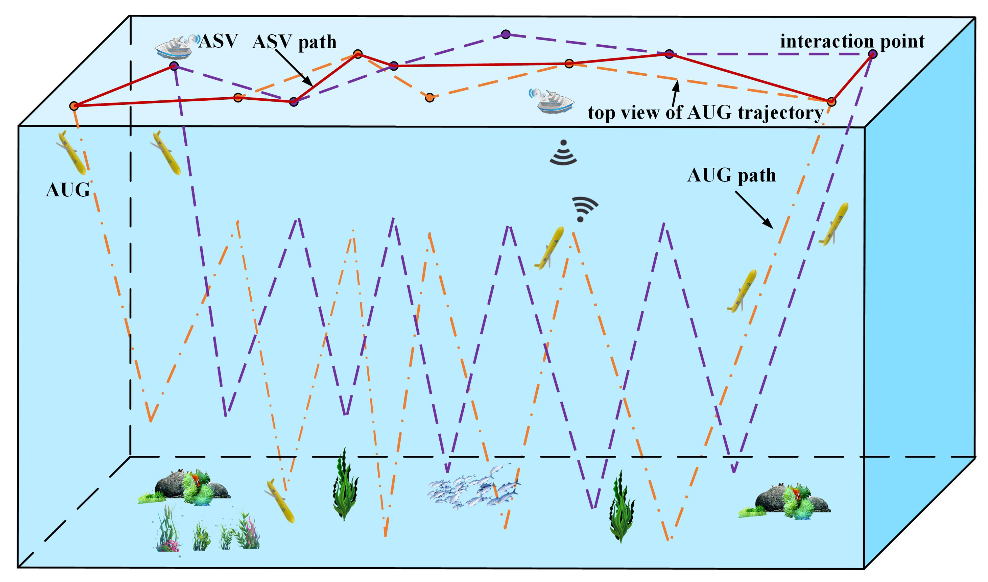
- A surface path planning method for underwater data collection with heterogeneous AMVs, named HSPP-HA, is proposed, which targets an application scenario where underwater data are collected through the collaboration of an ASV on the surface and multiple AUGs underwater based on underwater wireless communication and applies a modified SFLA to schedule the data collection between ASV and AUGs for the time-sensitive interactions between them;
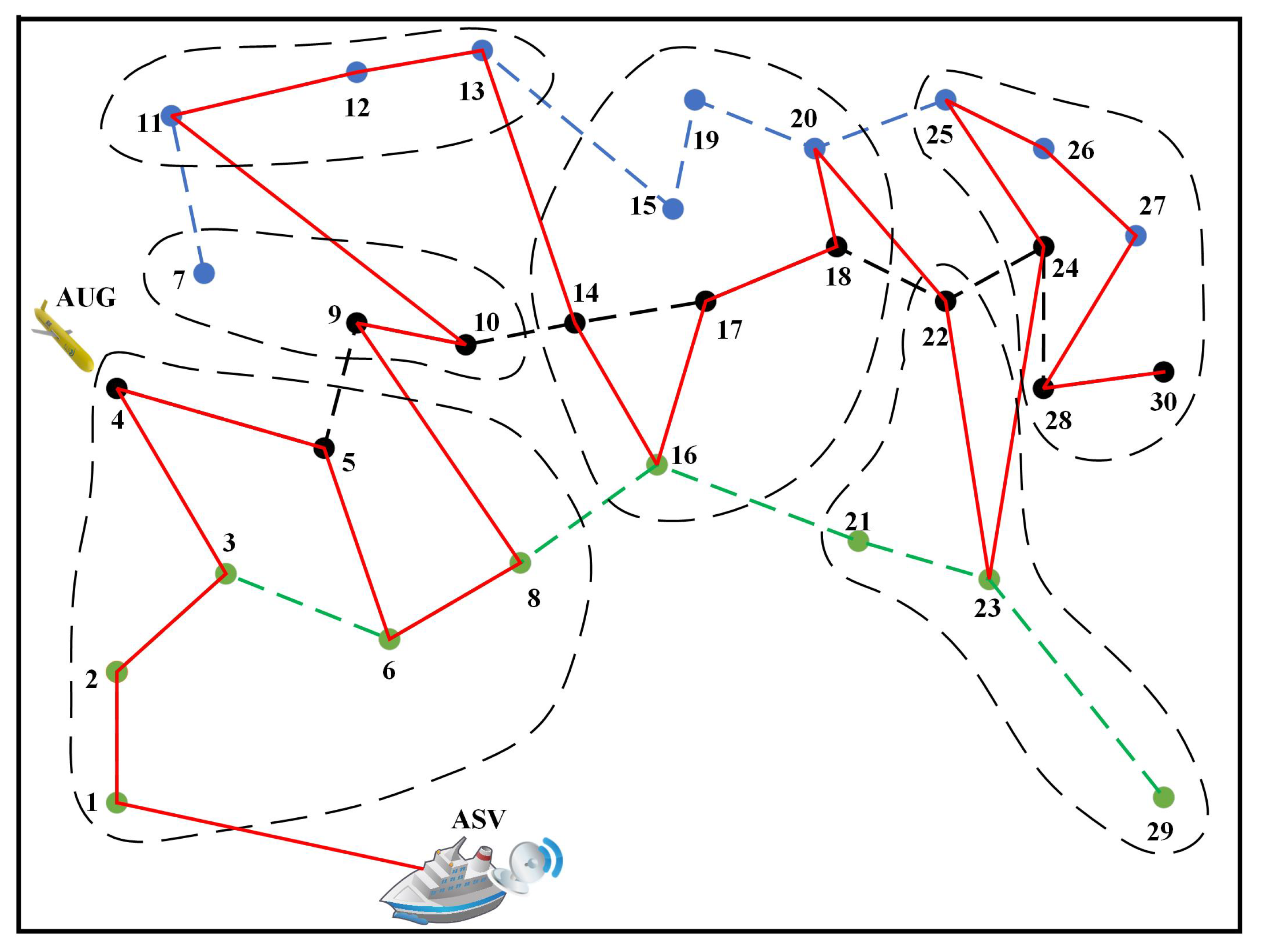
- An improved SFLA is designed with a spatial-temporal k-means algorithm and an adaptive iteration approach. The spatial-temporal k-means algorithm clusters the interaction points by their coordinates and times of occurrence to initialize the local searches; meanwhile, an adaptive iteration factor enables balanced local and global searches in optimizing the sequence of interactions and, furthermore, improves the convergence ability.
2. Related Works
3. System Model
3.1. Task Model
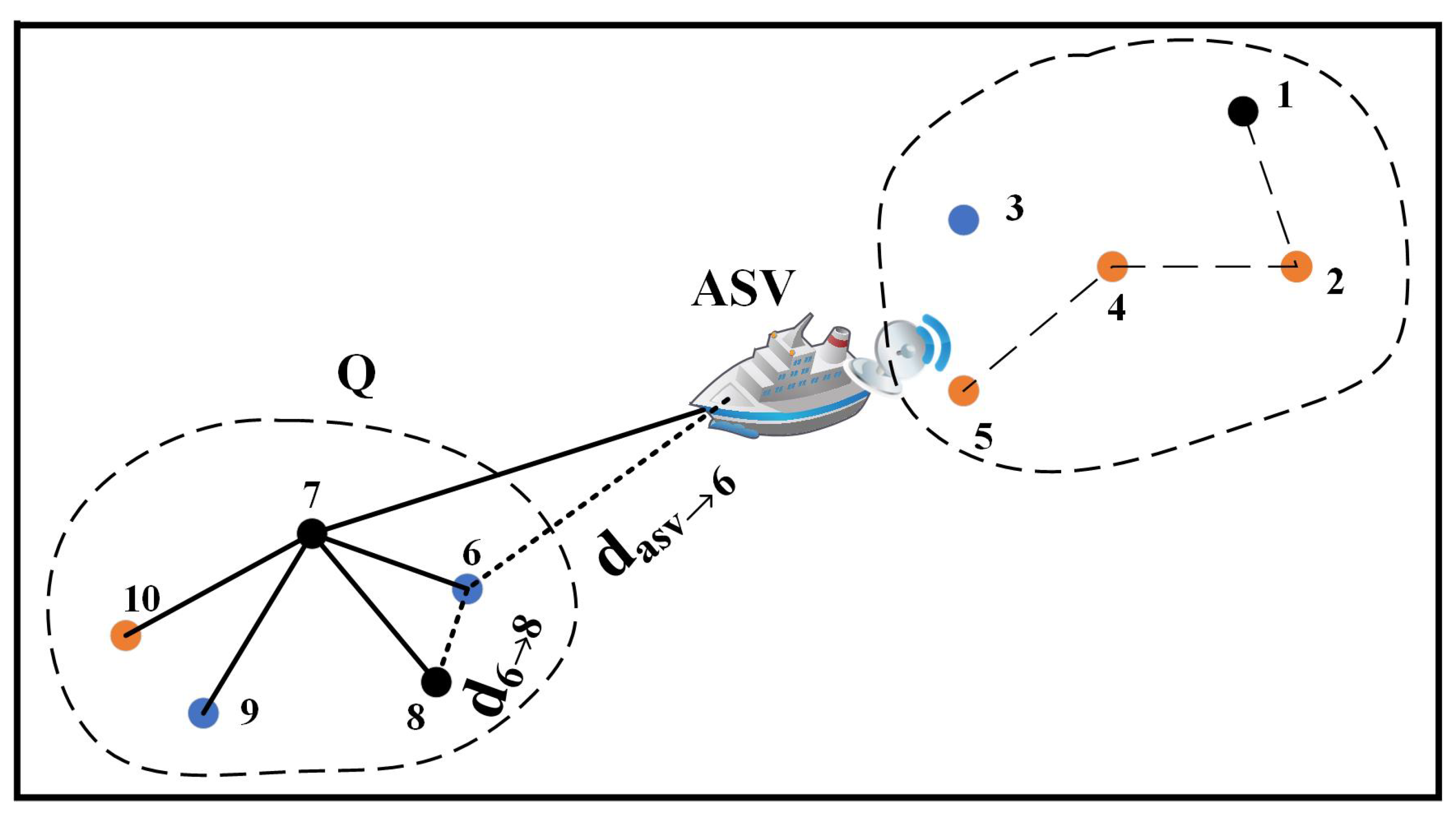
3.2. Constraint Model
3.3. Objective Optimization Model
4. Heuristic Surface Path Planning Method for Underwater Data Collection
4.1. Spatial-Temporal Clustering
| Algorithm 1: Spatial-temporal k-means clustering. |
 |
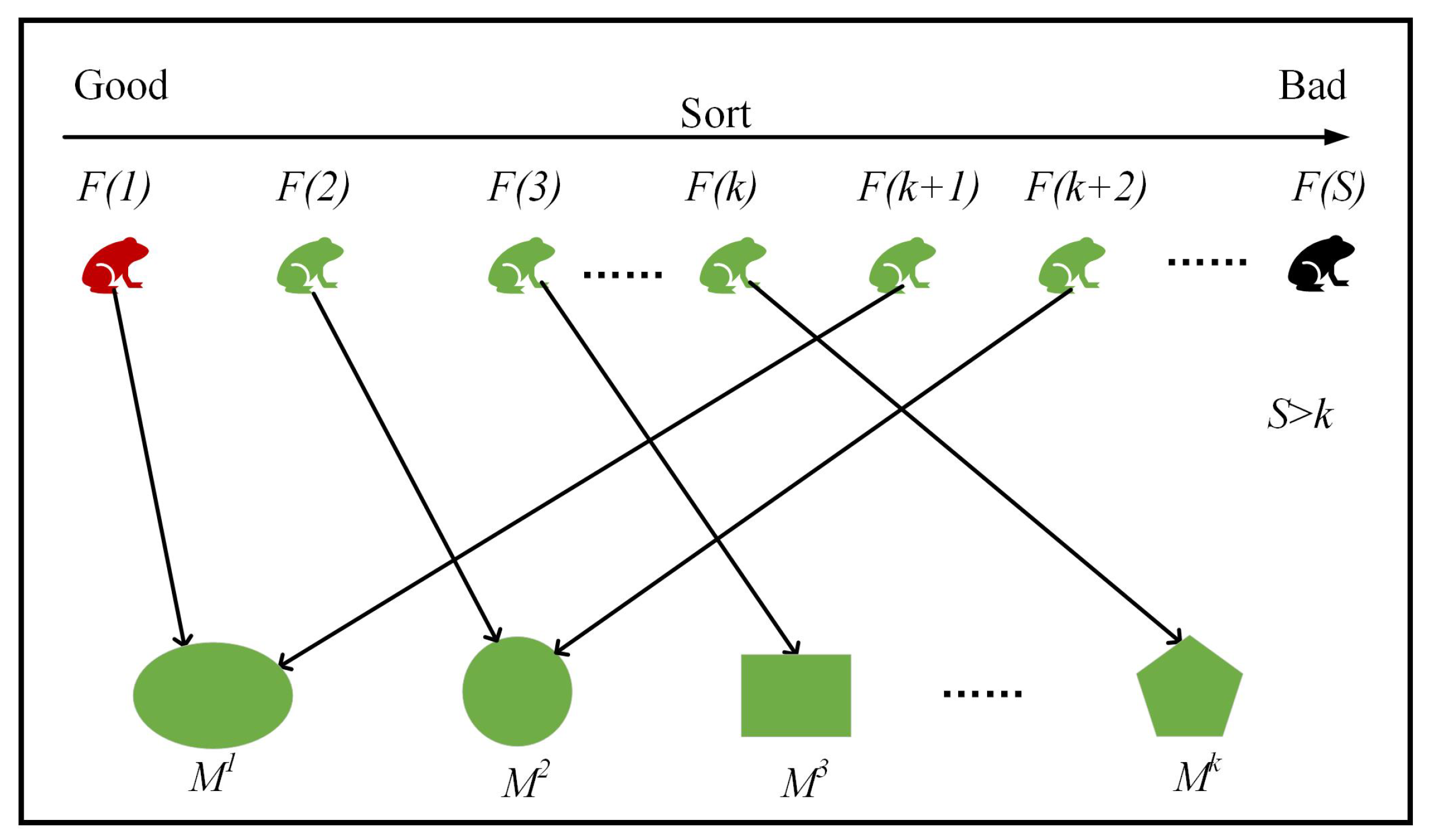
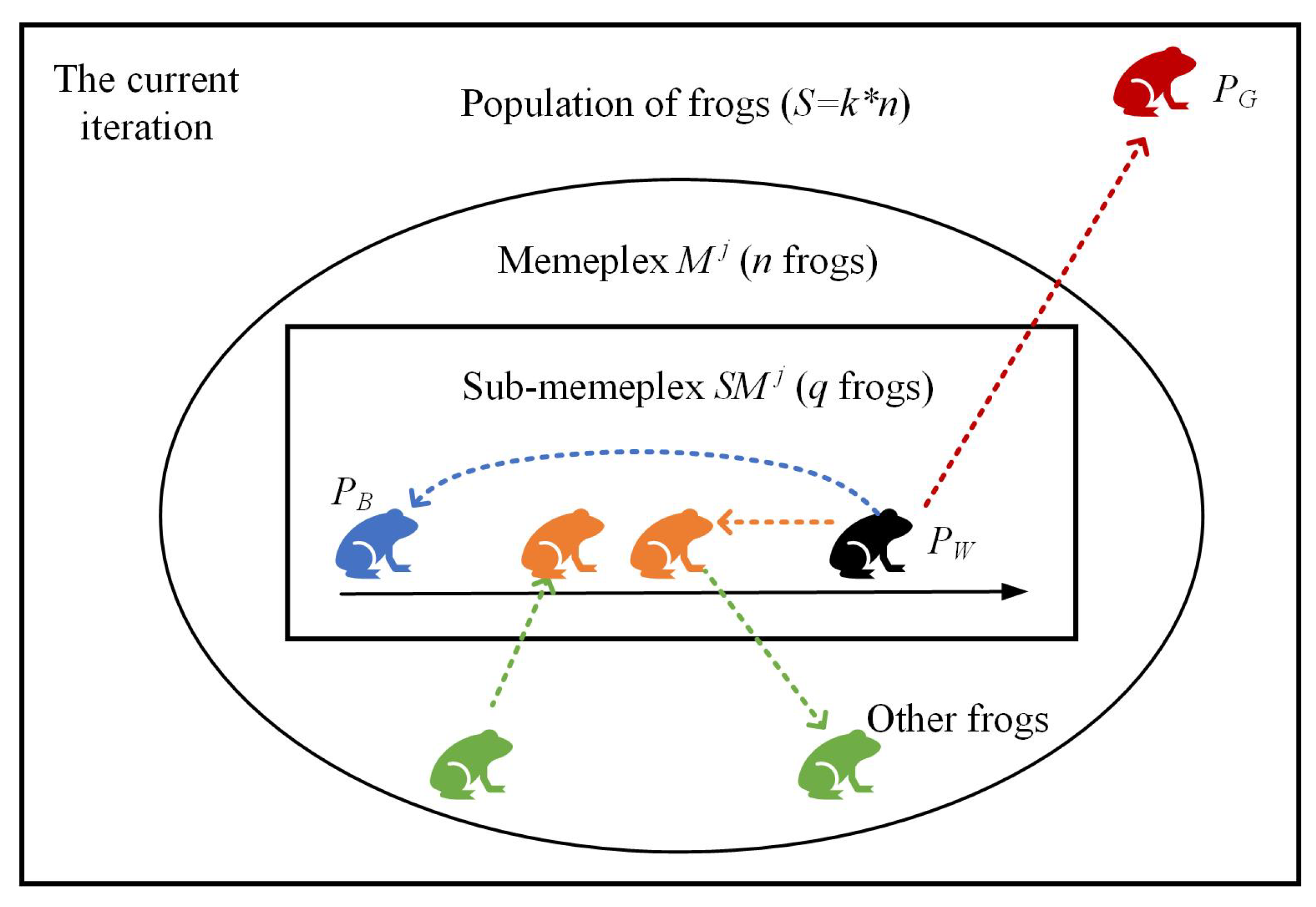
4.2. Shuffled Frog-Leaping with Adaptive Iteration Factor
| Algorithm 2: The overall process of HSPP-HA. |
 |
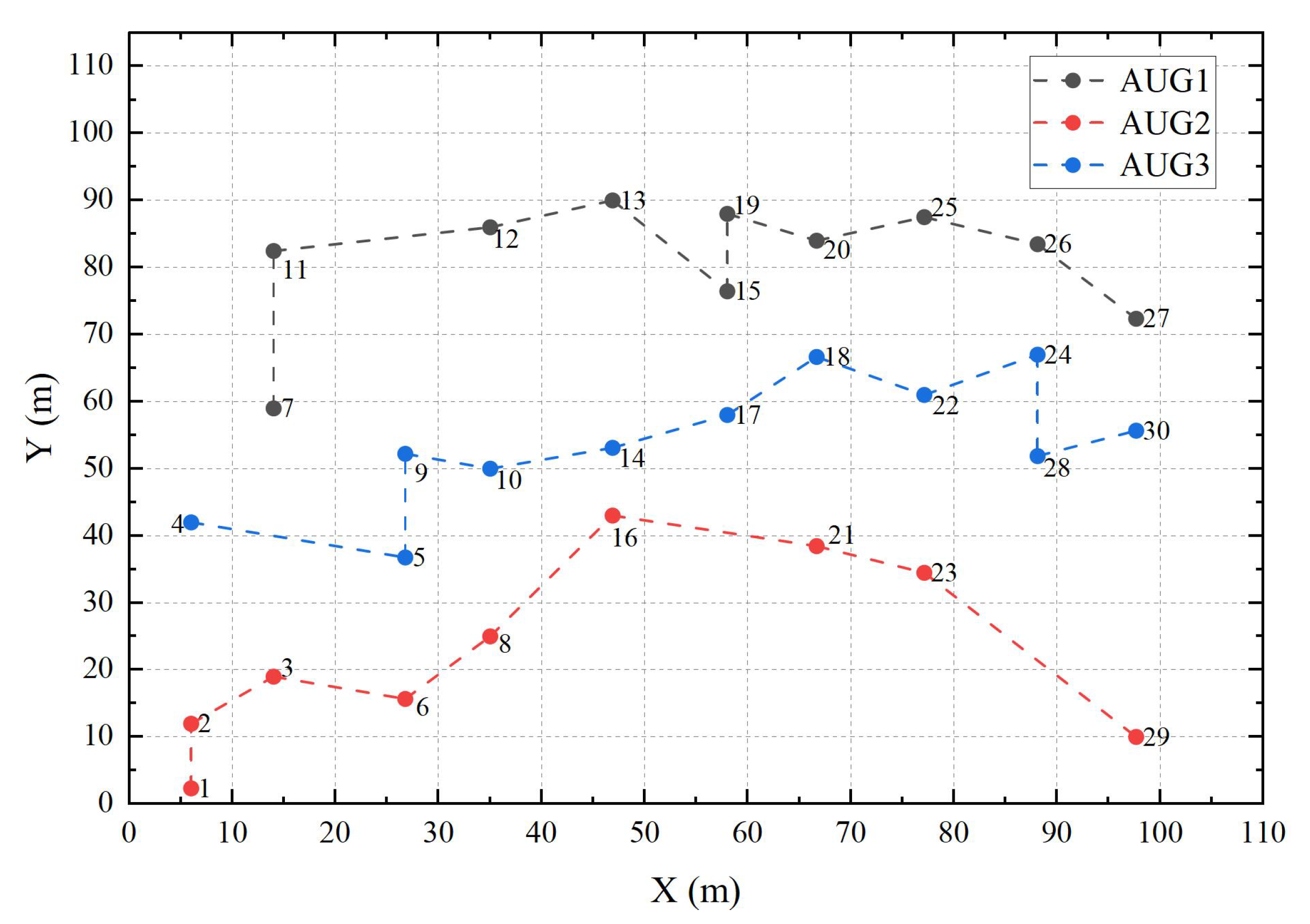
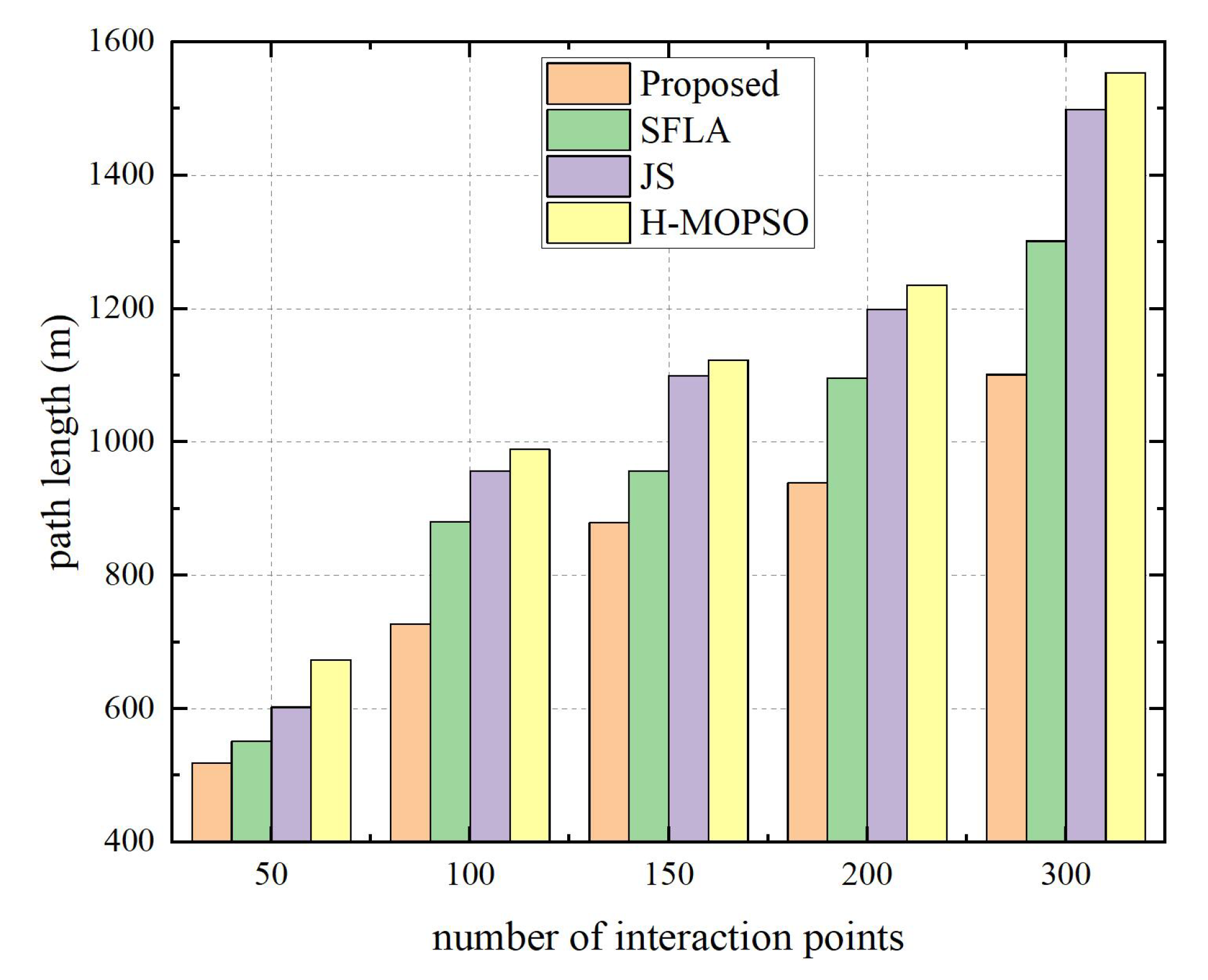
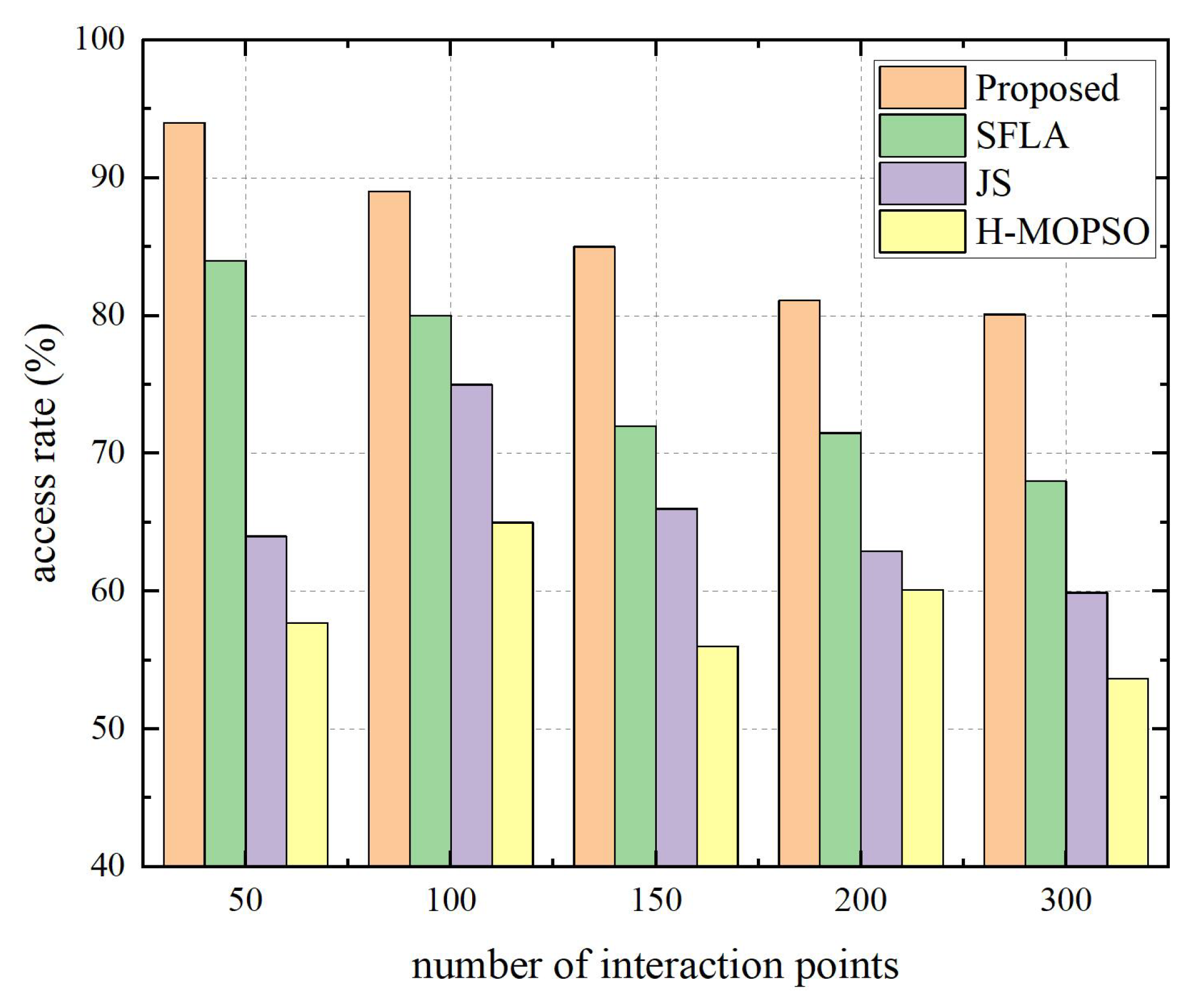
5. Simulation and Analysis
6. Conclusions
Author Contributions
Funding
Institutional Review Board Statement
Informed Consent Statement
Data Availability Statement
Conflicts of Interest
References
- Oceanix. Available online: https://oceanix.com/ (accessed on 1 January 2023).
- Tao, S.; Liu, H.; Wang, S.; Li, C. Construction of Smart Coastal Cities Based on Digital Government. J. Coast. Res. 2020, 110, 154–158. [Google Scholar] [CrossRef]
- Atham, S.B.; Guleria, K. Smart City in Underwater Wireless Sensor Networks. In Energy-Efficient Underwater Wireless Communications and Networking; IGI Global: Hershey, PA, USA, 2021; pp. 287–301. [Google Scholar]
- McMahon, J.; Plaku, E. Autonomous Data Collection With Dynamic Goals and Communication Constraints for Marine Vehicles. IEEE Trans. Autom. Sci. Eng. 2022, 1–14. [Google Scholar] [CrossRef]
- Han, G.; Qi, X.; Peng, Y.; Lin, C.; Zhang, Y.; Lu, Q. Early Warning Obstacle Avoidance-Enabled Path Planning for Multi-AUV-Based Maritime Transportation Systems. IEEE Trans. Intell. Transp. Syst. 2022. [Google Scholar] [CrossRef]
- Han, G.; Gong, A.; Wang, H.; Martínez-García, M.; Peng, Y. Multi-AUV Collaborative Data Collection Algorithm Based on Q-Learning in Underwater Acoustic Sensor Networks. IEEE Trans. Veh. Technol. 2021, 70, 9294–9305. [Google Scholar] [CrossRef]
- Chu, Z.; Wanf, F.; Lei, T.; Luo, C. Path Planning based on Deep Reinforcement Learning for Autonomous Underwater Vehicles under Ocean Current Disturbance. IEEE Trans. Intell. Veh. 2022, 8, 108–120. [Google Scholar] [CrossRef]
- Yang, J.; Huo, J.; Xi, M.; He, J.; Li, Z.; Song, H. A Time-saving Path Planning Scheme for Autonomous Underwater Vehicles with Complex Underwater Conditions. IEEE Internet Things J. 2023, 10, 1001–1013. [Google Scholar] [CrossRef]
- Zhang, J.; Sha, J.; Han, G.; Liu, J.; Qian, Y. A Cooperative-Control-Based Underwater Target Escorting Mechanism With Multiple Autonomous Underwater Vehicles for Underwater Internet of Things. IEEE Internet Things J. 2022, 8, 4403–4416. [Google Scholar] [CrossRef]
- Yu, F.; Chen, Y. Cyl-iRRT*: Homotopy Optimal 3D Path Planning for AUVs by Biasing the Sampling into a Cylindrical Informed Subset. IEEE Trans. Ind. Electron. 2022. [Google Scholar] [CrossRef]
- Wen, J.; Yang, J.; Li, Y.; He, J.; Li, Z.; Song, H. Behavior-Based Formation Control Digital Twin for Multi-AUG in Edge Computing. IEEE Trans. Netw. Sci. Eng. 2022. [Google Scholar] [CrossRef]
- Wen, J.; Yang, J.; Wei, W.; Lv, Z. Intelligent Multi-AUG Ocean Data Collection Scheme in Maritime Wireless Communication Network. IEEE Trans. Netw. Sci. Eng. 2022, 9, 3067–3079. [Google Scholar] [CrossRef]
- Hu, W.; Chen, F.; Xiang, L.; Chen, G. Multi-ASV Coordinated Tracking With Unknown Dynamics and Input Underactuation via Model-Reference Reinforcement Learning Control. IEEE Trans. Cybern. 2022, 1–10. [Google Scholar] [CrossRef] [PubMed]
- Jeong, M.; Lee, E.; Lee, M. An Adaptive Route Plan Technique with Risk Contour for Autonomous Navigation of Surface Vehicles. In Proceedings of the OCEANS MTS/IEEE Charleston, Charleston, SC, USA, 22–25 October 2018; pp. 1–4. [Google Scholar]
- Dubey, R.; Louis, S. VORRT-COLREGs: A Hybrid Velocity Obstacles and RRT Based COLREGs-Compliant Path Planner for Autonomous Surface Vessels. In Proceedings of the OCEANS 2021: San Diego—Porto, San Diego, CA, USA, 20–23 September 2021; pp. 1–8. [Google Scholar]
- Vagale, A.; Bye, R.; Osen, O. Evaluation of Path Planning Algorithms of Autonomous Surface Vehicles Based on Safety and Collision Risk Assessment. In Proceedings of the Global Oceans 2020: Singapore—U.S. Gulf Coast, Biloxi, MS, USA, 5–30 October 2020; pp. 1–8. [Google Scholar]
- Yu, Z.; Si, Z.; Li, X.; Wang, D.; Song, H. A Novel Hybrid Particle Swarm Optimization Algorithm for Path Planning of UAVs. IEEE Internet Things J. 2022, 9, 22547–22558. [Google Scholar] [CrossRef]
- Qadir, Z.; Zafar, M.; Moosavi, S.; Le, K.; Mahmud, M. Autonomous UAV Path-Planning Optimization Using Metheuristic Approach for Predisaster Assessment. IEEE Internet Things J. 2022, 9, 12505–12514. [Google Scholar] [CrossRef]
- Kaveh, A.; Dadras, A. A novel meta-heuristic optimization algorithm: Thermal exchange optimization. Adv. Eng. Softw. 2017, 110, 69–84. [Google Scholar] [CrossRef]
- Kaveh, A.; Dadras Eslamlou, A. Water strider algorithm: A new metaheuristic and applications. Structures 2020, 25, 520–541. [Google Scholar] [CrossRef]
- Muzaffar, E.; Kevin, L.; Fayzul, P. Shuffled frog-leaping algorithm: A memetic meta-heuristic for discrete optimization. Eng. Optim. 2006, 38, 129–154. [Google Scholar]
- Yang, J.; Ni, J.; Xi, M.; Wen, J.; Li, Y. Intelligent Path Planning of Underwater Robot Based on Reinforcement Learning. IEEE Trans. Autom. Sci. Eng. 2022. [Google Scholar] [CrossRef]
- Abbasi, A.; MahmoudZadeh, S.; Yazdani, A. A Cooperative Dynamic Task Assignment Framework for COTSBot AUVs. IEEE Trans. Autom. Sci. Eng. 2022, 19, 1163–1179. [Google Scholar] [CrossRef]
- Scott, D.; Manyam, S.; Casbeer, D.; Kumar, M. A Lagrangian Algorithm for Multiple Depot Traveling Salesman Problem With Revisit Period Constraints. IEEE Trans. Autom. Sci. Eng. 2022. [Google Scholar] [CrossRef]
- Chen, M.; Zhu, D. A Workload Balanced Algorithm for Task Assignment and Path Planning of Inhomogeneous Autonomous Underwater Vehicle System. IEEE Trans. Cogn. Dev. Syst. 2019, 11, 483–493. [Google Scholar] [CrossRef]
- Zhu, D.; Zhou, B.; Yang, S. A Novel Algorithm of Multi-AUVs Task Assignment and Path Planning Based on Biologically Inspired Neural Network Map. IEEE Trans. Intell. Veh. 2021, 6, 333–342. [Google Scholar] [CrossRef]
- Wu, J.; Song, C.; Ma, J.; Wu, J.; Han, G. Reinforcement Learning and Particle Swarm Optimization Supporting Real-Time Rescue Assignments for Multiple Autonomous Underwater Vehicles. IEEE Trans. Intell. Transp. Syst. 2022, 23, 6807–6820. [Google Scholar] [CrossRef]
- Wang, N.; Xu, H. Dynamics-Constrained Global-Local Hybrid Path Planning of an Autonomous Surface Vehicle. IEEE Trans. Veh. Technol. 2020, 69, 6928–6942. [Google Scholar] [CrossRef]
- Hu, L.; Naeem, W.; Rajabally, E.; Watson, G.; Mills, T.; Bhuiyam, Z.; Raeburn, C.; Salter, I.; Pekcan, C. A Multiobjective Optimization Approach for COLREGs-Compliant Path Planning of Autonomous Surface Vehicles Verified on Networked Bridge Simulators. IEEE Trans. Intell. Transp. Syst. 2020, 21, 1167–1179. [Google Scholar] [CrossRef]
- Jian, S.; Hsieh, S. A Niching Regression Adaptive Memetic Algorithm for Multimodal Optimization of the Euclidean Traveling Salesman Problem. IEEE TRansactions Evol. Comput. 2022. [Google Scholar] [CrossRef]
- Xin, C.; Kang, W.; Yi, M.; Zheng, L.; Jun, Z.; Qing, Z. Decomposition-based Lin-Kernighan Heuristic with Neighborhood Structure Transfer for Multi/Many-objective Traveling Salesman Problem. IEEE Trans. Evol. Comput. 2022. [Google Scholar] [CrossRef]
- Zhang, Z.; Liu, H.; Zhou, M.; Wang, J. Solving Dynamic Traveling Salesman Problems With Deep Reinforcement Learning. IEEE Trans. Neural Netw. Learn. Syst. 2021. [Google Scholar] [CrossRef] [PubMed]
- Sanyal, S.; Roy, K. Neuro-Ising: Accelerating Large-Scale Traveling Salesman Problems via Graph Neural Network Guided Localized Ising Solvers. IEEE Trans. Comput.-Aided Des. Integr. Circuits Syst. 2022, 41, 5408–5420. [Google Scholar] [CrossRef]
- Mei, H.; Wang, H.; Shen, X.; Bai, W. An Adaptive MAC Protocol for Underwater Acoustic Sensor Networks With Dynamic Traffic. In Proceedings of the OCEANS MTS/IEEE Charleston of the Conference, Charleston, SC, USA, 22–25 October 2018; pp. 1–4. [Google Scholar]
- Qiao, G.; Zhao, Y.; Liu, S.; Ahmed, N. The Effect of Acoustic-Shell Coupling on Near-End Self-Interference Signal of In-Band Full-Duplex Underwater Acoustic Communication Modem. In Proceedings of the 17th International Bhurban Conference on Applied Sciences and Technology (IBCAST) of the Conference, Natl Ctr Phys, Islamabad, Pakistan, 14–18 January 2020; pp. 606–610. [Google Scholar]
- Eghbal, M.; Saha, T.; Hasan, K. Transmission expansion planning by meta-heuristic techniques: A comparison of Shuffled Frog Leaping Algorithm, PSO and GA. In Proceedings of the 2011 IEEE Power and Energy Society General Meeting of the Conference, Detroit, MI, USA, 24–28 July 2011; pp. 1–8. [Google Scholar]
- Duarte, B.; de Oliveira, L.; Teixeira, M.; Barbosa, M. A comparison of Genetic and Memetic Algorithms applied to the Traveling Salesman Problem with Draft Limits. In Proceedings of the 47th Latin American Computing Conference (CLEI) of the Conference, Cartago, Costa Rica, 25–29 October 2021. [Google Scholar]
- Huang, M.; Zhang, K.; Zeng, Z.; Wang, T.; Liu, Y. An AUV-Assisted Data Gathering Scheme Based on Clustering and Matrix Completion for Smart Ocean. IEEE Internet Things J. 2020, 7, 9904–9918. [Google Scholar] [CrossRef]
- Jui, C.; Dinh, T. A novel metaheuristic optimizer inspired by behavior of jellyfish in ocean. Appl. Math. Comput. 2021, 289, 125535. [Google Scholar]


| Parameters | Definition |
|---|---|
| Clustered memeplexes, | |
| k | Number of clusters |
| n | Number of frogs in a cluster |
| S | Frog populations = |
| A frog, | |
| Path fitness value of a frog, | |
| q | Number of selected frogs in a local search |
| Sub-memeplex with q frogs, | |
| Leaping vector of the best frog in each iteration | |
| Leaping vector of the local optimal frog in an | |
| Leaping vector of the local worst frog in an | |
| The local worst frog in an | |
| New frog after updates, | |
| Path fitness value of , |
| Algorithms | Parameters | Values |
|---|---|---|
| JS | ||
| SFLA | ||
| H-MOPSO | ||
| Proposed | ||
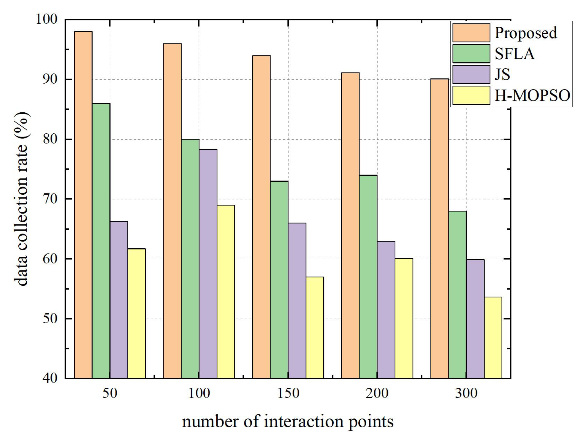
| Algorithms | Number of Interaction Points | Path Length (m) | Access Rate (%) | Data Collection Rate (%) | Time Complexity |
|---|---|---|---|---|---|
| H-MOPSO | 30 | 547.80 | 76.67 | 86.67 | |
| 100 | 989.35 | 65.00 | 69.00 | ||
| 200 | 1234.68 | 60.00 | 60.00 | ||
| JS | 30 | 501.30 | 66.67 | 93.33 | |
| 100 | 956.49 | 75.00 | 78.00 | ||
| 200 | 1199.16 | 63.00 | 62.00 | ||
| SFLA | 30 | 436.80 | 70.00 | 93.33 | |
| 100 | 880.41 | 80.00 | 80.00 | ||
| 200 | 1096.13 | 71.00 | 74.00 | ||
| Proposed | 30 | 411.60 | 73.33 | 100.00 | |
| 100 | 727.58 | 89.00 | 96.00 | ||
| 200 | 939.23 | 82.00 | 90.00 |
Disclaimer/Publisher’s Note: The statements, opinions and data contained in all publications are solely those of the individual author(s) and contributor(s) and not of MDPI and/or the editor(s). MDPI and/or the editor(s) disclaim responsibility for any injury to people or property resulting from any ideas, methods, instructions or products referred to in the content. |
© 2023 by the authors. Licensee MDPI, Basel, Switzerland. This article is an open access article distributed under the terms and conditions of the Creative Commons Attribution (CC BY) license (https://creativecommons.org/licenses/by/4.0/).
Share and Cite
Zhang, J.; Wang, Z.; Han, G.; Qian, Y. Heuristic Surface Path Planning Method for AMV-Assisted Internet of Underwater Things. Sustainability 2023, 15, 3137. https://doi.org/10.3390/su15043137
Zhang J, Wang Z, Han G, Qian Y. Heuristic Surface Path Planning Method for AMV-Assisted Internet of Underwater Things. Sustainability. 2023; 15(4):3137. https://doi.org/10.3390/su15043137
Chicago/Turabian StyleZhang, Jie, Zhengxin Wang, Guangjie Han, and Yujie Qian. 2023. "Heuristic Surface Path Planning Method for AMV-Assisted Internet of Underwater Things" Sustainability 15, no. 4: 3137. https://doi.org/10.3390/su15043137