
A Spatial Model of Landslides with A Micro-Topography and Vegetation Approach for Sustainable Land Management in the Volcanic Area

Abstract
:1. Introduction
2. Materials and Methods
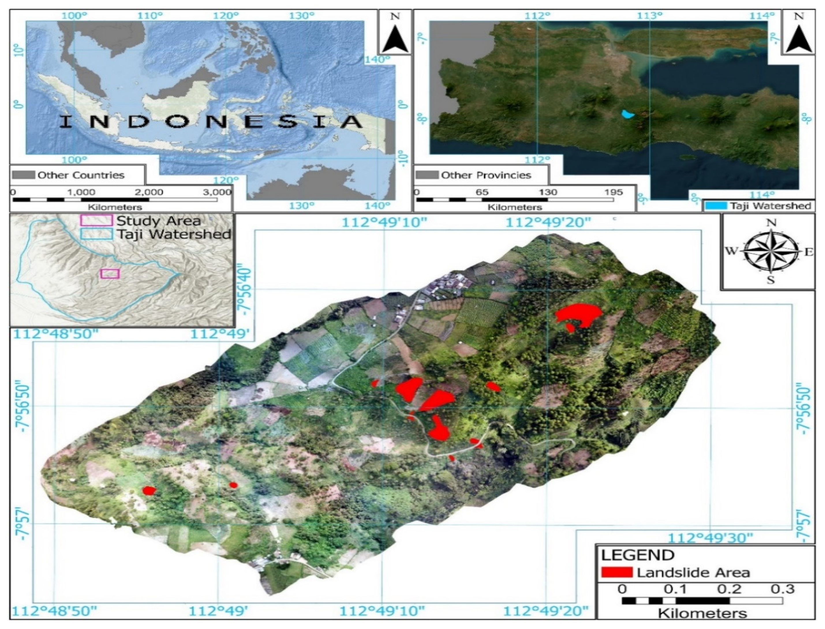
2.1. Study Area
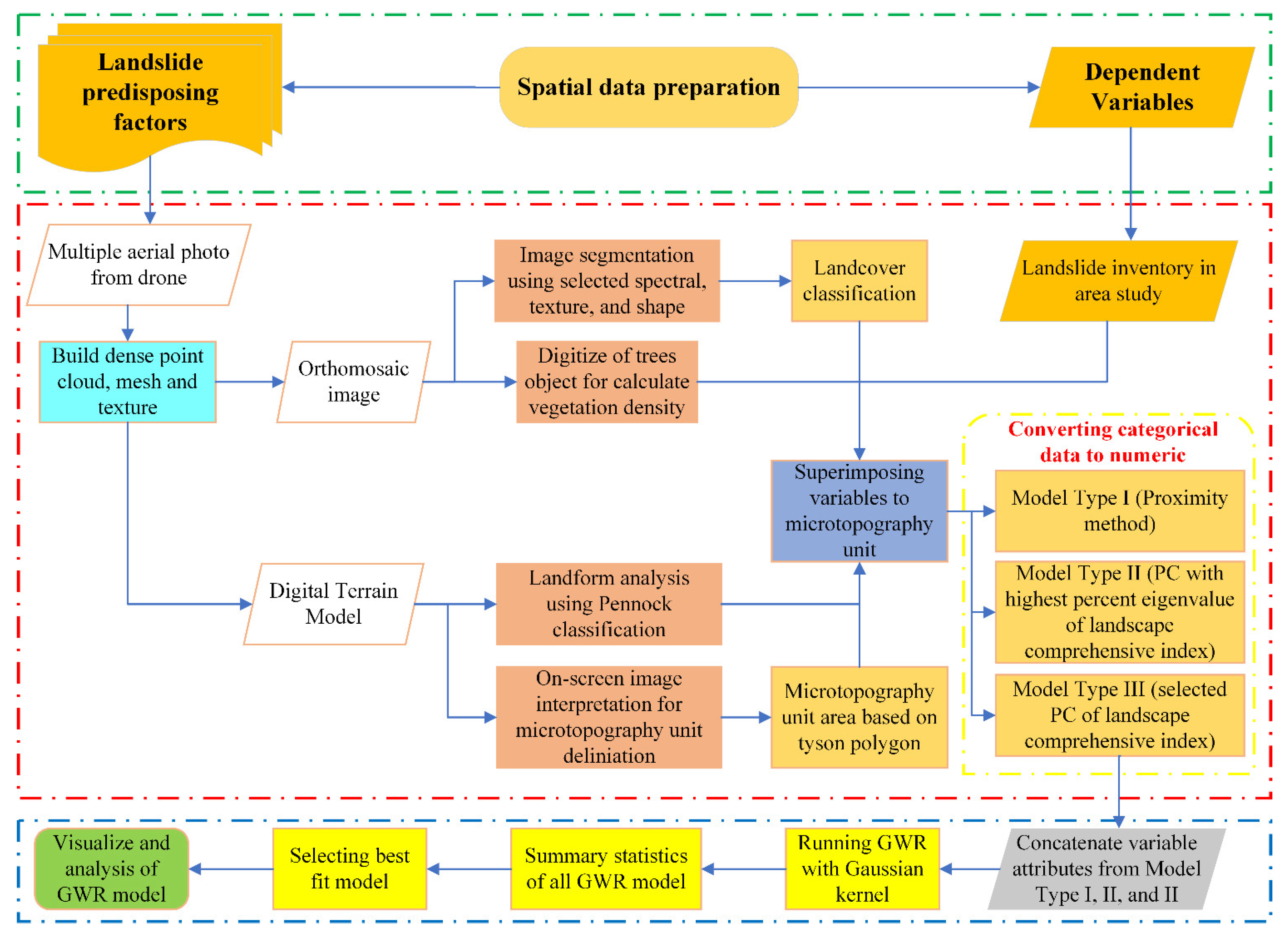
2.2. Methodology
2.3. Data Collection and Processing
2.3.1. Orthomosaic Image and Digital Terrain Model (DTM) from Unmanned Aerial Vehicle (UAV)
2.3.2. Landslide Inventory
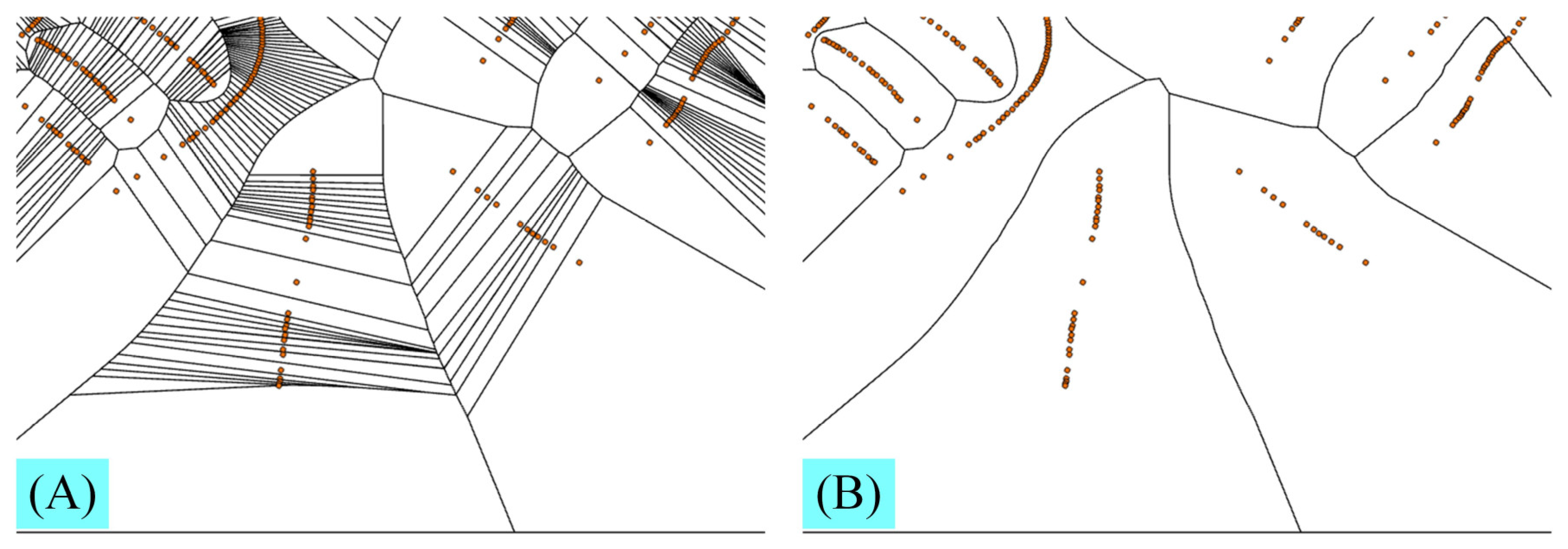
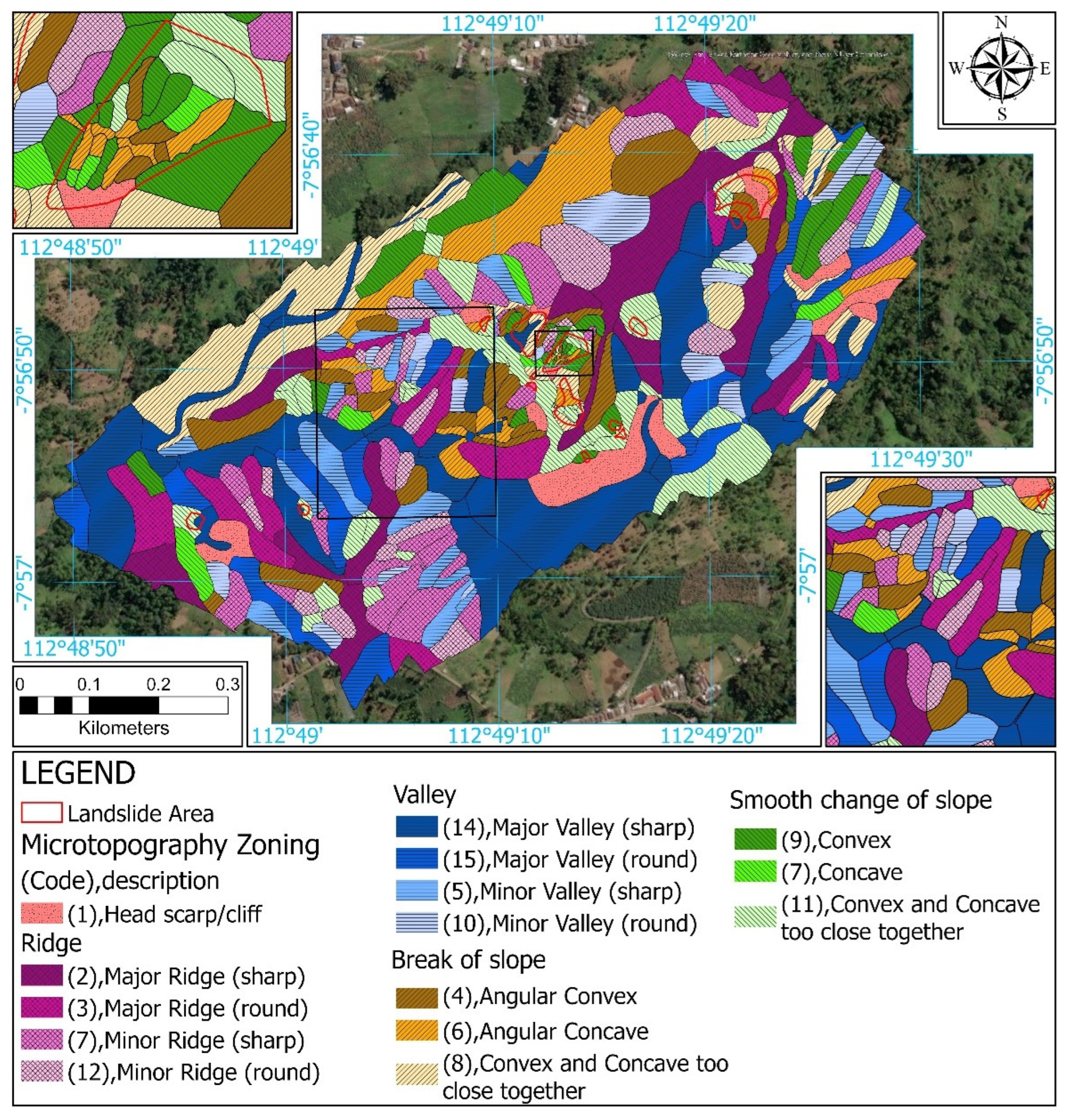
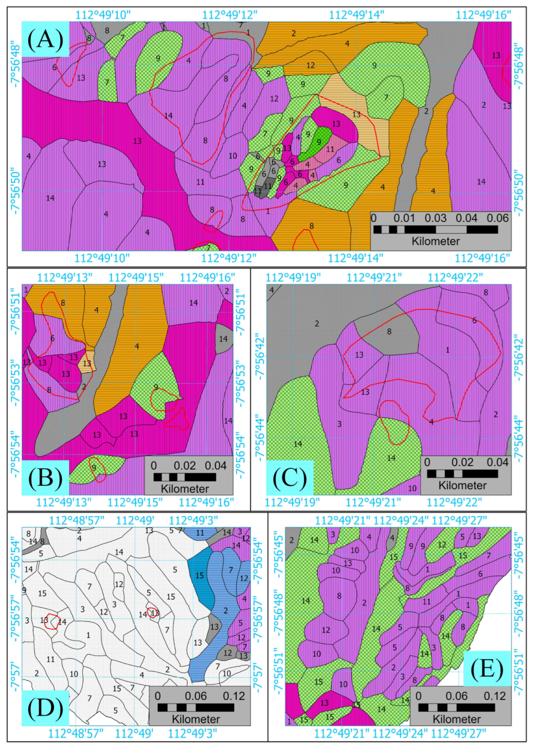
2.3.3. Microtopographic Zoning
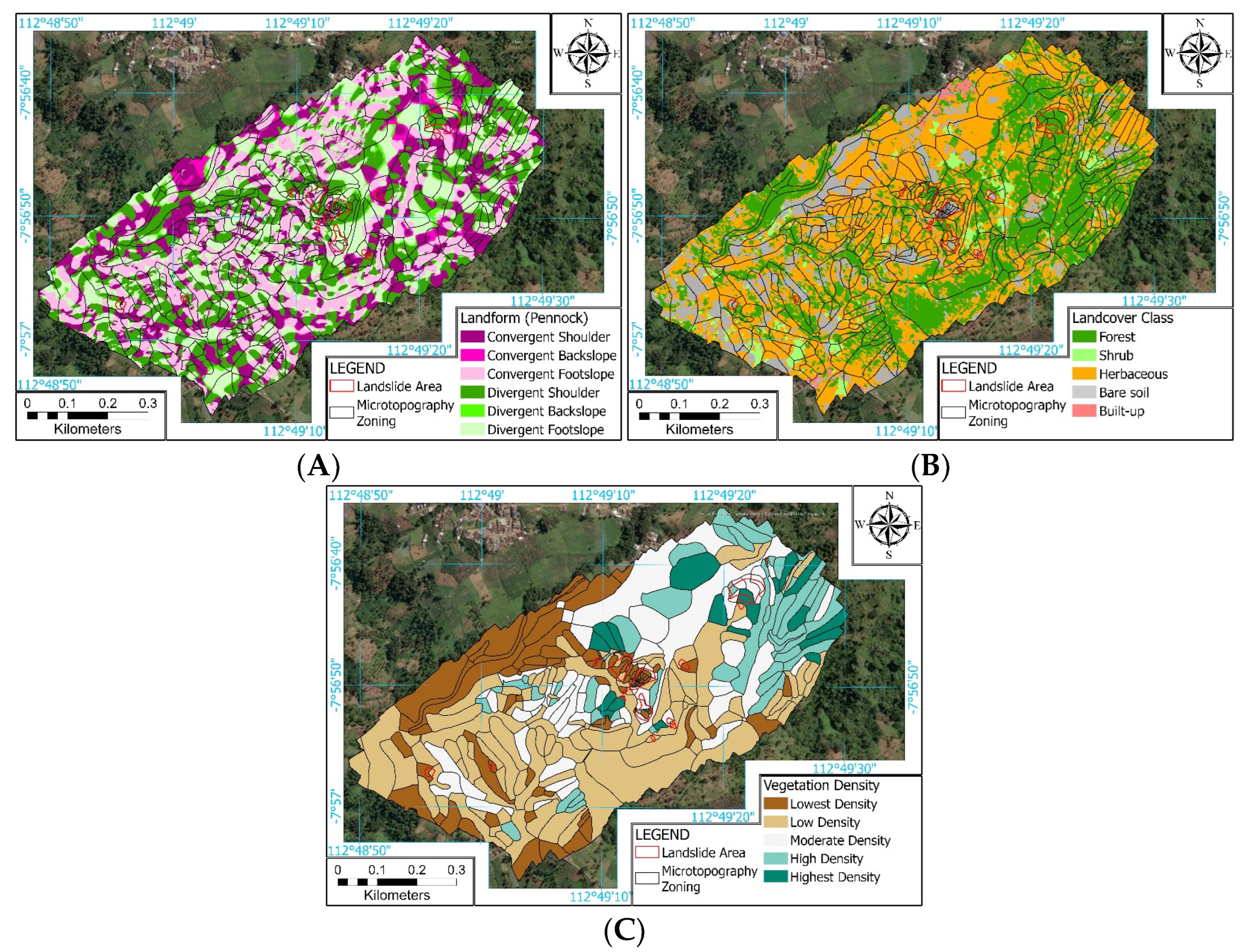
2.3.4. Landforms of the Pennock Classification System
2.3.5. Land Cover Classification
2.3.6. Vegetation Density
2.4. Transformation of Categorical Data into Numeric on Microtopography, Landform and Land Cover
2.4.1. Type I Data Transformation
2.4.2. Type II Data Transformation
2.4.3. Type III Data Transformation
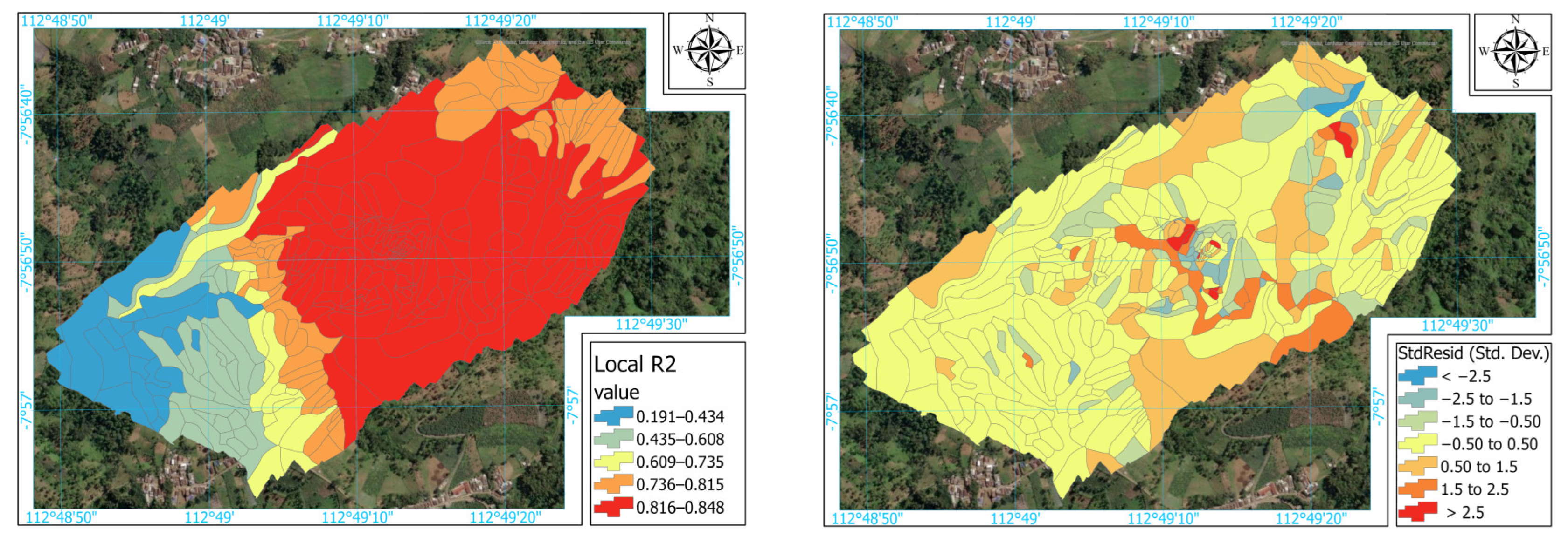
2.5. Geographically Weighted Regression Model Analysis
3. Results
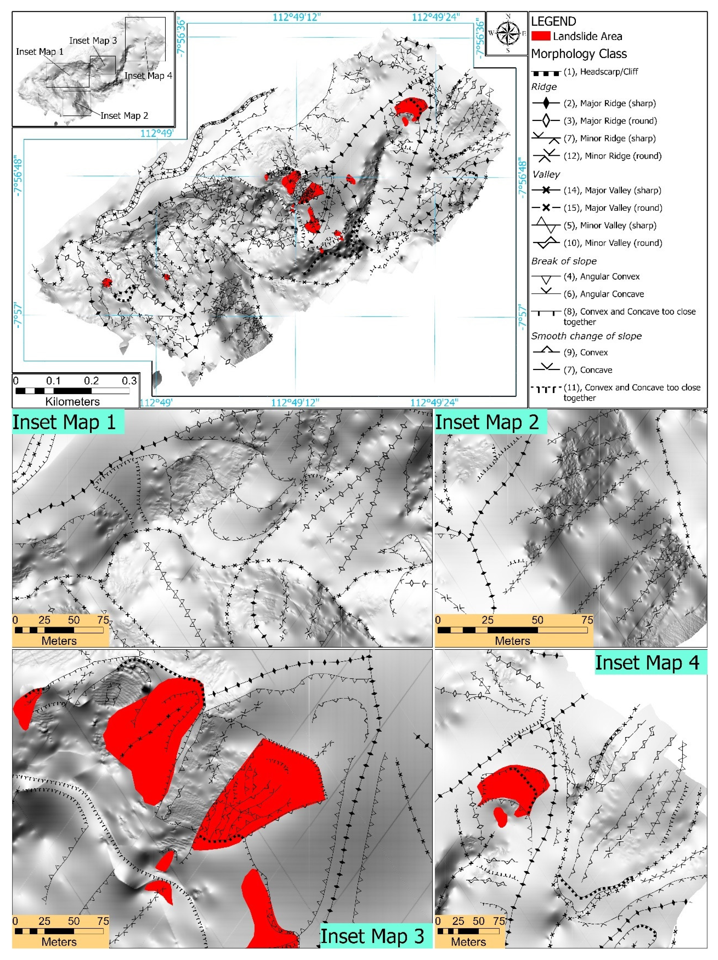
3.1. Results of Mapping Microtopographic Zoning, Landforms, Land Cover, and Vegetation Density
3.2. Comprehensive Index Analysis of Landscape Metrics on Landform and Land Cover
3.3. Model the Local Spatial Relationship between the Landslide and the Selected Independent Variable Model Type for Priority Land Management Sustainability
4. Discussion
4.1. Mapping Microtopography, Landforms, Land Cover, and Vegetation Density
4.2. GWR Model Implementation with Different Independent Variable Data Transformation
4.3. Modeling Local Spatial Relationships of Landslides
4.4. Research Implications and Limitations
5. Conclusions
Author Contributions
Funding
Institutional Review Board Statement
Informed Consent Statement
Data Availability Statement
Conflicts of Interest
References
- Chalise, D.; Kumar, L.; Kristiansen, P. Land degradation by soil erosion in Nepal: A review. Soil Syst. 2019, 3, 12. [Google Scholar] [CrossRef]
- Kirui, O.K.; Mirzabaev, A.; von Braun, J. Assessment of land degradation ‘on the ground’ and from ‘above’. SN Appl. Sci. 2021, 3, 318. [Google Scholar] [CrossRef]
- Chasek, P. From land degradation to land restoration. Policy Briefs 2022, 29, 2. [Google Scholar]
- AGU. The Human Cost of Landslides in 2016. The Landslide Blog—AGU Blogosphere. 2017. Available online: https://blogs.agu.org/landslideblog/2017/01/30/human-cost-of-landslides-2016/ (accessed on 7 January 2023).
- BNPB. Data Informasi Bencana Indonesia (DIBI). 2008. Available online: https://gis.bnpb.go.id/ (accessed on 7 January 2023).
- Setiawan, H.; Wilopo, W.; Wiyoso, T.; Fathani, T.F.; Karnawati, D. Investigation and numerical simulation of the 22 February 2018 landslide-triggered long-traveling debris flow at Pasir Panjang Village, Brebes Regency of Central Java, Indonesia. Landslides 2019, 16, 2219–2232. [Google Scholar] [CrossRef]
- Karnawati, D.; Fathani, T.F.; Ignatius, S.; Andayani, B.; Legono, D.; Burton, P.W. Landslide hazard and community-based risk reduction effort in Karanganyar and the surrounding area, central Java, Indonesia. J. Mt. Sci. 2011, 8, 149–153. [Google Scholar] [CrossRef]
- Bachr, I.S.; Stötter, J.; Monreal, M.; Sartohadi, J. The calamity of eruptions, or an eruption of benefits? Mt. Bromo human–volcano system a case study of an open-risk perception. Nat. Hazards Earth Syst. Sci. 2015, 15, 277–290. [Google Scholar] [CrossRef]
- Marc, O.; Stumpf, A.; Malet, J.-P.; Gosset, M.; Uchida, T.; Chiang, S.-H. Initial insights from a global database of rainfall-induced landslide inventories: The weak influence of slope and strong influence of total storm rainfall. Earth Surf. Dyn. 2018, 6, 903–922. [Google Scholar] [CrossRef]
- Bachri, S.; Shrestha, R.P.; Yulianto, F.; Sumarmi, S.; Utomo, K.S.B.; Aldianto, Y.E. Mapping Landform and Landslide Susceptibility Using Remote Sensing, GIS and Field Observation in the Southern Cross Road, Malang Regency, East Java, Indonesia. Geosciences 2020, 11, 4. [Google Scholar] [CrossRef]
- Van Westen, C.J.; Soeters, R.; Sijmons, K. Digital geomorphological landslide hazard mapping of the Alpago area, Italy. Int. J. Appl. Earth Obs. Geoinf. 2000, 2, 51–60. [Google Scholar] [CrossRef]
- Mallet, C.; David, N. Digital Terrain Models Derived from Airborne LiDAR Data. In Optical Remote Sensing of Land Surface; Elsevier: Amsterdam, The Netherlands, 2016; pp. 299–319. [Google Scholar]
- Tempa, K.; Peljor, K.; Wangdi, S.; Ghalley, R.; Jamtsho, K.; Ghalley, S.; Pradhan, P. UAV technique to localize landslide susceptibility and mitigation proposal: A case of Rinchending Goenpa landslide in Bhutan. Nat. Hazards Res. 2021, 1, 171–186. [Google Scholar] [CrossRef]
- Pellicani, R.; Argentiero, I.; Manzari, P.; Spilotro, G.; Marzo, C.; Ermini, R.; Apollonio, C. UAV and Airborne LiDAR Data for Interpreting Kinematic Evolution of Landslide Movements: The Case Study of the Montescaglioso Landslide (Southern Italy). Geosciences 2019, 9, 248. [Google Scholar] [CrossRef]
- Granados-Bolaños, S.; Quesada-Román, A.; Alvarado, G.E. Low-cost UAV applications in dynamic tropical volcanic landforms. J. Volcanol. Geotherm. Res. 2021, 410, 107143. [Google Scholar] [CrossRef]
- Sofia, G. Combining geomorphometry, feature extraction techniques and Earth-surface processes research: The way forward. Geomorphology 2020, 355, 107055. [Google Scholar] [CrossRef]
- Nagamatsu, D.; Miura, O. Soil disturbance regime in relation to micro-scale landforms and its effects on vegetation structure in a hilly area in Japan. Plant Ecol. 1997, 133, 191–200. [Google Scholar] [CrossRef]
- Chimner, R.A.; Hart, J.B. Hydrology and microtopography effects on northern white-cedar regeneration in Michigan’s Upper Peninsula. Can. J. For. Res. 1996, 26, 389–393. [Google Scholar] [CrossRef]
- Schaetzl, R.J.; Follmer, L.R. Longevity of treethrow microtopography: Implications for mass wasting. Geomorphology 1990, 3, 113–123. [Google Scholar] [CrossRef]
- Kabrick, J.M.; Meyers, N.L.; McSweeney, K. Comparison of Sampling Methods for Estimating Pit and Mound Microtopography. Soil Sci. Soc. Am. J. 1997, 61, 1423–1427. [Google Scholar] [CrossRef]
- Wang, J.; Zhu, Q.K.; Qin, W.; Zhang, H.Z.; Yun, L.; Xie, J.; Kuang, G.M. Differentiation of vegetation characteristics on slope micro-topography of fenced watershed in loess area of north Shaanxi province, Northwest China. J. Appl. Ecol. 2012, 23, 694–700. [Google Scholar]
- Zhu, Q.K.; Zhang, Y.; Zhao, L.L. Vegetation Restoration and Simulated Natural Forestation in the Loess Plateau, Northern Shaanxi, China; Beijing Science Press: Beijing, China, 2012. [Google Scholar]
- Zhao, W.; Zhang, Y.; Zhu, Q.; Qin, W.; Peng, S.; Li, P.; Zhao, Y.; Ma, H.; Wang, Y. Effects of microtopography on spatial point pattern of forest stands on the semi-arid Loess Plateau, China. J. Arid Land 2015, 7, 370–380. [Google Scholar] [CrossRef]
- Sakai, A.; Ohsawa, M. Topographical pattern of the forest vegetation on a river basin in a warm-temperate hilly region, central Japan. Ecol. Res. 1994, 9, 269–280. [Google Scholar] [CrossRef]
- Sakai, A.; Ohsawa, M. Vegetation pattern and microtopography on a landslide scar of Mt Kiyosumi, central Japan. Ecol. Res. 1993, 8, 47–56. [Google Scholar] [CrossRef]
- Knight, J.; Mitchell, W.A.; Rose, J. Geomorphological Field Mapping. In Geomorphological Mapping Methods and Application, 1st ed.; Smith, M.J., Paron, P., Griffiths, J.S., Eds.; Elsevier: Amsterdam, Netherlands, 2011; pp. 151–187. [Google Scholar]
- Pisano, L.; Zumpano, V.; Malek, Ž.; Rosskopf, C.M.; Parise, M. Variations in the susceptibility to landslides, as a consequence of land cover changes: A look to the past, and another towards the future. Sci. Total Environ. 2017, 601, 1147–1159. [Google Scholar] [CrossRef] [PubMed]
- Pourghasemi, H.; Gayen, A.; Park, S.; Lee, C.-W.; Lee, S. Assessment of Landslide-Prone Areas and Their Zonation Using Logistic Regression, LogitBoost, and NaïveBayes Machine-Learning Algorithms. Sustainability. 2018, 10, 3697. [Google Scholar] [CrossRef]
- Jones, S.; Kasthurba, A.K.; Bhagyanathan, A.; Binoy, B.V. Impact of anthropogenic activities on landslide occurrences in southwest India: An investigation using spatial models. J. Earth Syst. Sci. 2021, 130, 70. [Google Scholar] [CrossRef]
- Shu, H.; Hürlimann, M.; Molowny-Horas, R.; González, M.; Pinyol, J.; Abancó, C.; Ma, J. Relation between land cover and landslide susceptibility in Val d’Aran, Pyrenees (Spain): Historical aspects, present situation and forward prediction. Sci. Total Environ. 2019, 693, 133557. [Google Scholar] [CrossRef]
- Akgun, A.; Türk, N. Landslide susceptibility mapping for Ayvalik (Western Turkey) and its vicinity by multicriteria decision analysis. Environ. Earth Sci. 2010, 61, 595–611. [Google Scholar] [CrossRef]
- Castellanos Abella, E.A.; van Westen, C.J. Qualitative landslide susceptibility assessment by multicriteria analysis: A case study from San Antonio del Sur, Guantánamo, Cuba. Geomorphology 2008, 94, 453–466. [Google Scholar] [CrossRef]
- Guzzetti, F.; Carrara, A.; Cardinali, M.; Reichenbach, P. Landslide hazard evaluation: A review of current techniques and their application in a multi-scale study, Central Italy. Geomorphology 1999, 31, 181–216. [Google Scholar] [CrossRef]
- Zhang, W.; Liu, S.; Wang, L.; Samui, P.; Chwała, M.; He, Y. Landslide Susceptibility Research Combining Qualitative Analysis and Quantitative Evaluation: A Case Study of Yunyang County in Chongqing, China. Forests 2022, 13, 1055. [Google Scholar] [CrossRef]
- Pourghasemi, H.R.; Kariminejad, N.; Gayen, A.; Komac, M. Statistical functions used for spatial modelling due to assessment of landslide distribution and landscape-interaction factors in Iran. Geosci. Front. 2020, 11, 1257–1269. [Google Scholar] [CrossRef]
- Brunsdon, C.; Fotheringham, S.; Charlton, M. Geographically Weighted Regression. J. R. Stat. Soc. Ser. D Stat. 1998, 47, 431–443. [Google Scholar] [CrossRef]
- Wang, H.B.; Sassa, K. Comparative evaluation of landslide susceptibility in Minamata area, Japan. Environ. Geol. 2005, 47, 956–966. [Google Scholar] [CrossRef]
- Pix4D. Pix4Dcapture; Pix4D: Renens, Switzerland, 2022; Available online: https://www.pix4d.com/ (accessed on 1 August 2022).
- Dandois, J.; Olano, M.; Ellis, E. Optimal Altitude, Overlap, and Weather Conditions for Computer Vision UAV Estimates of Forest Structure. Remote Sens. 2015, 7, 13895–13920. [Google Scholar] [CrossRef]
- Agisoft LLC. Agisoft PhotoScan; Agisoft LLC: Saint Petersburg, Russia, 2022; Available online: https://www.agisoft.com/ (accessed on 1 August 2022).
- Kaimaris, D.; Patias, P.; Sifnaiou, M. UAV and the comparison of image processing software. Int. J. Intell. Unmanned Syst. 2017, 5, 18–27. [Google Scholar] [CrossRef]
- Nebiker, S.; Lack, N.; Deuber, M. Building Change Detection from Historical Aerial Photographs Using Dense Image Matching and Object-Based Image Analysis. Remote Sens. 2014, 6, 8310–8336. [Google Scholar] [CrossRef]
- Goodbody, T.; Coops, N.; Hermosilla, T.; Tompalski, P.; Pelletier, G. Vegetation Phenology Driving Error Variation in Digital Aerial Photogrammetrically Derived Terrain Models. Remote Sens. 2018, 10, 1554. [Google Scholar] [CrossRef]
- Yilmaz, V.; Konakoglu, B.; Serifoglu, C.; Gungor, O.; Gökalp, E. Image classification-based ground filtering of point clouds extracted from UAV-based aerial photos. Geocarto Int. 2018, 33, 310–320. [Google Scholar] [CrossRef]
- Cooke, R.U.; Doornkamp, J.C. Geomorphology in Environmental Management; Clarendon Press: Oxford, UK, 1974. [Google Scholar]
- Rashid, I.; Romshoo, S.A.; Hajam, J.A.; Abdullah, T. A semi-automated approach for mapping geomorphology in mountainous terrain, Ferozpora watershed (Kashmir Himalaya). J. Geol. Soc. India 2016, 88, 206–212. [Google Scholar] [CrossRef]
- Yang, H.; Zhao, Z.; Jiang, C.; Wen, Y.; Muneeb Abid, M. Spatially Varying Relation between Built Environment and Station-Level Subway Passenger-Distance. J. Adv. Transp. 2022, 2022, 1–18. [Google Scholar] [CrossRef]
- Pennock, D.J.; Zebarth, B.J.; de Jong, E. Landform classification and soil distribution in hummocky terrain, Saskatchewan, Canada. Geoderma 1987, 40, 297–315. [Google Scholar] [CrossRef]
- Evans, D.A.; Williard, K.W.J.; Schoonover, J.E. Comparison of Terrain Indices and Landform Classification Procedures in Low-Relief Agricultural Fields. J. Geospat. Appl. Nat. Resour. 2016, 1, 1. [Google Scholar]
- Pradhan, B.; Chaudhari, A.; Adinarayana, J.; Buchroithner, M.F. Soil erosion assessment and its correlation with landslide events using remote sensing data and GIS: A case study at Penang Island, Malaysia. Environ. Monit. Assess. 2012, 184, 715–727. [Google Scholar] [CrossRef] [PubMed]
- Blaschke, T. Object based image analysis for remote sensing. ISPRS J. Photogramm. Remote Sens. 2010, 65, 2–16. [Google Scholar] [CrossRef]
- Modica, G.; de Luca, G.; Messina, G.; Praticò, S. Comparison and assessment of different object-based classifications using machine learning algorithms and UAVs multispectral imagery: A case study in a citrus orchard and an onion crop. Eur. J. Remote Sens. 2021, 54, 431–460. [Google Scholar] [CrossRef]
- BBlaschke, T.; Hay, G.J.; Kelly, M.; Lang, S.; Hofmann, P.; Addink, E.; Feitosa, R.Q.; van der Meer, F.; van der Werff, H.; van Coillie, F.; et al. Geographic Object-Based Image Analysis—Towards a new paradigm. ISPRS J. Photogramm. Remote Sens. 2014, 87, 180–191. [Google Scholar] [CrossRef]
- Torres-Sánchez, J.; López-Granados, F.; Peña, J.M. An automatic object-based method for optimal thresholding in UAV images: Application for vegetation detection in herbaceous crops. Comput. Electron. Agric. 2015, 114, 43–52. [Google Scholar] [CrossRef]
- De Castro, A.; Torres-Sánchez, J.; Peña, J.; Jiménez-Brenes, F.; Csillik, O.; López-Granados, F. An Automatic Random Forest-OBIA Algorithm for Early Weed Mapping between and within Crop Rows Using UAV Imagery. Remote Sens. 2018, 10, 285. [Google Scholar] [CrossRef]
- Hall, M.A.; Holmes, G. Benchmarking attribute selection techniques for discrete class data mining. IEEE Trans. Knowl. Data Eng. 2003, 15, 1437–1447. [Google Scholar] [CrossRef]
- Ma, L.; Fu, T.; Blaschke, T.; Li, M.; Tiede, D.; Zhou, Z.; Ma, X.; Chen, D. Evaluation of Feature Selection Methods for Object-Based Land Cover Mapping of Unmanned Aerial Vehicle Imagery Using Random Forest and Support Vector Machine Classifiers. ISPRS Int. J. Geo-Inf. 2017, 6, 51. [Google Scholar] [CrossRef]
- Breiman, L. Random Forests. Mach. Learn. 2001, 45, 5–32. [Google Scholar] [CrossRef]
- Li, M.; Ma, L.; Blaschke, T.; Cheng, L.; Tiede, D. A systematic comparison of different object-based classification techniques using high spatial resolution imagery in agricultural environments. Int. J. Appl. Earth Obs. Geoinf. 2016, 49, 87–98. [Google Scholar] [CrossRef]
- Ma, L.; Li, M.; Ma, X.; Cheng, L.; Du, P.; Liu, Y. A review of supervised object-based land-cover image classification. ISPRS J. Photogramm. Remote Sens. 2017, 130, 277–293. [Google Scholar] [CrossRef]
- De Luca, G.N.; Silva, J.M.; Cerasoli, S.; Araújo, J.; Campos, J.; di Fazio, S.; Modica, G. Object-Based Land Cover Classification of Cork Oak Woodlands using UAV Imagery and Orfeo ToolBox. Remote Sens. 2019, 11, 1238. [Google Scholar] [CrossRef]
- Stehman, S.V. Estimating the kappa coefficient and its variance under stratified random sampling. Photogramm. Eng. Remote Sens. 1996, 62, 401–407. [Google Scholar]
- Congalton, R.G.; Green, K. Assessing the Accuracy of Remotely Sensed Data; CRC Press: Boca Raton, FL, USA, 2019. [Google Scholar]
- McGarigal, K.; Cushman, S.A.; Neel, M.C.; Ene, E. FRAGSTATS: Spatial Pattern Analysis Program for Categorical Maps. Computer Software Program Produced by the Authors at the University of Massachusetts, Amherst. 2002. Available online: https://fragstats.software.informer.com/4.2/ (accessed on 23 July 2022).
- Schultz, C.; Alegría, A.C.; Cornelis, J.; Sahli, H. Comparison of spatial and aspatial logistic regression models for landmine risk mapping. Appl. Geogr. 2016, 66, 52–63. [Google Scholar] [CrossRef]
- Alzaga, V.; Tizzani, P.; Acevedo, P.; Ruiz-Fons, F.; Vicente, J.; Gortázar, C. Deviance partitioning of host factors affecting parasitization in the European brown hare (Lepus europaeus). Naturwissenschaften 2009, 96, 1157–1168. [Google Scholar] [CrossRef] [PubMed]
- Romero, D.; Olivero, J.; Real, R. Comparative assessment of different methods for using land-cover variables for distribution modelling of Salamandra salamandra longirotris. Environ. Conserv. 2013, 40, 48–59. [Google Scholar] [CrossRef]
- Uuemaa, E.; Mander, Ü.; Marja, R. Trends in the use of landscape spatial metrics as landscape indicators: A review. Ecol Indic. 2013, 28, 100–106. [Google Scholar] [CrossRef]
- Wang, X.; Zhang, F. Multi-scale analysis of the relationship between landscape patterns and a water quality index (WQI) based on a stepwise linear regression (SLR) and geographically weighted regression (GWR) in the Ebinur Lake oasis. Environ. Sci. Pollut. Res. 2018, 25, 7033–7048. [Google Scholar] [CrossRef]
- Dinesh, S. Analysis of Landform Metrics of Mountains Extracted from Multiscale Digital Elevation Models. Aust. J. Basic Appl. Sci. 2009, 3, 3997–4010. [Google Scholar]
- Galicia, L.; Zarco-Arista, A.E.; Mendoza-Robles, K.I.; Palacio-Prieto, J.L.; García-Romero, A. Land use/cover, landforms and fragmentation patterns in a tropical dry forest in the southern Pacific region of Mexico. Singap. J. Trop. Geogr. 2008, 29, 137–154. [Google Scholar] [CrossRef]
- Ramachandra, T.V.; Bharath, A.H.; Sowmyashree, M.V. Monitoring urbanization and its implications in a mega city from space: Spatiotemporal patterns and its indicators. J. Environ. Manag. 2015, 148, 67–81. [Google Scholar] [CrossRef] [PubMed]
- Hesselbarth, M.H.K.; Sciaini, M.; With, K.A.; Wiegand, K.; Nowosad, J. Landscapemetrics: An open-source R tool to calculate landscape metrics. Ecography 2019, 42, 1648–1657. [Google Scholar] [CrossRef]
- Frazier, A.E.; Kedron, P. Landscape Metrics: Past Progress and Future Directions. Curr. Landsc. Ecol. Rep. 2017, 2, 63–72. [Google Scholar] [CrossRef]
- Liu, S.; Li, X.; Chen, L.; Zhao, Q.; Zhao, C.; Hu, X.; Li, J. A New Approach to Investigate the Spatially Heterogeneous in the Cooling Effects of Landscape Pattern. Land 2022, 11, 239. [Google Scholar] [CrossRef]
- Odhiambo Omuya, E.; Onyango Okeyo, G.; Waema Kimwele, M. Feature Selection for Classification using Principal Component Analysis and Information Gain. Expert Syst. Appl. 2021, 174, 114765. [Google Scholar] [CrossRef]
- Kononenko, I. Estimating attributes: Analysis and extensions of RELIEF. In ECML-94; Bergadano, F., de Raedt, L., Eds.; Machine Learning; Springer: Berlin/Heidelberg, Germany, 1994; pp. 171–182. [Google Scholar]
- Kira, K.; Rendell, L.A. A Practical Approach to Feature Selection. In Machine Learning Proceedings 1992; Sleeman, D., Edwards, P., Eds.; Elsevier: Amsterdam, The Netherlands, 1992; pp. 249–256. [Google Scholar]
- Fotheringham, A.S.; Brunsdon, C.; Charlton, M. Geographically Weighted Regression: The Analysis of Spatially Varying Relationships; John Wiley & Sons: Hoboken, NJ, USA, 2002. [Google Scholar]
- Li, Y.; Liu, X.; Han, Z.; Dou, J. Spatial Proximity-Based Geographically Weighted Regression Model for Landslide Susceptibility Assessment: A Case Study of Qingchuan Area, China. Appl. Sci. 2020, 10, 1107. [Google Scholar] [CrossRef]
- Yang, X.; Tang, G.; Meng, X.; Xiong, L. Classification of Karst Fenglin and Fengcong Landform Units Based on Spatial Relations of Terrain Feature Points from DEMs. Remote Sens. 2019, 11, 1950. [Google Scholar] [CrossRef]
- Prasannakumar, V.; Vijith, H.; Geetha, N. Terrain evaluation through the assessment of geomorphometric parameters using DEM and GIS: Case study of two major sub-watersheds in Attapady, South India. Arab. J. Geosci. 2013, 6, 1141–1151. [Google Scholar] [CrossRef]
- Lillesand, T.M.; Kiefer, R.W. Remote Sensing and Image Interpretation, 4th ed.; John Wiley & Sons: New York, NY, USA, 2000; p. 469. [Google Scholar]
- Hu, X.; Xu, C.; Chen, J.; Lin, Y.; Lin, S.; Wu, Z.; Qiu, R. A Synthetic Landscape Metric to Evaluate Urban Vegetation Quality: A Case of Fuzhou City in China. Forests 2022, 13, 1002. [Google Scholar] [CrossRef]
- Jolliffe, I.T. A Note on the Use of Principal Components in Regression. Appl. Stat. 1982, 31, 300. [Google Scholar] [CrossRef]
- Mason, R.L.; Gunst, R.F. Selecting principal components in regression. Stat. Probab. Lett. 1985, 3, 299–301. [Google Scholar] [CrossRef]
- Hadi, A.S.; Ling, R.F. Some Cautionary Notes on the Use of Principal Components Regression. Am. Stat. 1998, 52, 15–19. [Google Scholar]
- Sato, H.P.; Hasegawa, H.; Fujiwara, S.; Tobita, M.; Koarai, M.; Une, H.; Iwahashi, J. Interpretation of landslide distribution triggered by the 2005 Northern Pakistan earthquake using SPOT 5 imagery. Landslides 2007, 4, 113–122. [Google Scholar] [CrossRef]
- Wang, H.B.; Li, J.M.; Zhou, B.; Zhou, Y.; Yuan, Z.Q.; Chen, Y.P. Application of a hybrid model of neural networks and genetic algorithms to evaluate landslide susceptibility. Geoenvironmental Disasters 2017, 4, 15. [Google Scholar] [CrossRef]
- Havenith, H.-B.; Strom, A.; Caceres, F.; Pirard, E. Analysis of landslide susceptibility in the Suusamyr region, Tien Shan: Statistical and geotechnical approach. Landslides 2006, 3, 39–50. [Google Scholar] [CrossRef]
- Ray, R.L.; Jacobs, J.M. Relationships among remotely sensed soil moisture, precipitation and landslide events. Nat. Hazards 2007, 43, 211–222. [Google Scholar] [CrossRef]


| Profile Curvature (°/m) | Kemiringan Lereng (°) | Plan Curvature (°/m) | Elemen Bentuklahan |
|---|---|---|---|
| Concave (<−0.10) Linear (>−0.10, <0.10) Convex (>0.10) | >3.0 | Concave (<0.0) | Convergent Shoulder |
| >3.0 | Concave (<0.0) | Convergent Backslope | |
| >3.0 | Concave (<0.0) | Convergent Footslope | |
| >3.0 | Convex (>0.0) | Divergent Shoulder | |
| >3.0 | Convex (>0.0) | Divergent Backslope | |
| >3.0 | Convex (>0.0) | Divergent Footslope |
| Metrik | Rumus | Range |
|---|---|---|
| Aggregation index (AI) | ||
| Class area (CA) | ||
| Clumpiness index (CLUMPY) | ||
| Patch cohesion index (COHESION) | ||
| Landscape division index (DIVISION) | ||
| Edge density (ED) | ||
| Largest patch index (LPI) | ||
| Landscape shape index (LSI) | ||
| Number of patches (NP) | ||
| Patch density (PD) | ||
| Percentage of class (PLAND) |
| Landcover | Forest | Shrub | Herbaceous | Bare Soil | Built-up | Total | User Accuracy (%) |
|---|---|---|---|---|---|---|---|
| Forest | 816 | 0 | 2 | 1 | 0 | 819 | 99.63 |
| Shrub | 4 | 177 | 5 | 1 | 0 | 187 | 94.65 |
| Herbaceous | 7 | 0 | 1050 | 2 | 0 | 1059 | 99.15 |
| Bare soil | 7 | 0 | 7 | 371 | 0 | 385 | 96.36 |
| Built-up | 3 | 0 | 3 | 3 | 125 | 134 | 93.28 |
| Total | 837 | 177 | 1067 | 378 | 125 | Overall = 98.26% | |
| Producer Accuracy (%) | 97.49 | 100 | 98.4 | 98.15 | 100 | Kappa = 0.97 | |
| LF1 | LF2 | LF3 | LF4 | LF5 | LF6 | ||
|---|---|---|---|---|---|---|---|
| PC1 | Eigen | 4.18 | 4.52 | 3.89 | 3.81 | 4.99 | 4.51 |
| % Eigen | 37.98% | 41.12% | 35.42% | 34.64% | 45.44% | 40.96% | |
| AM | 0.0147 | −0.0005 | −0.0003 | 0.009 | −0.0002 | 0.0094 | |
| PC2 | Eigen | 2.36 | 2.19 | 2.28 | 2.58 | 1.9 | 2.23 |
| % Eigen | 21.44% | 19.86% | 20.74% | 23.48% | 17.30% | 20.29% | |
| AM | 0.0059 | 0.01218 | −0.0041 | 0.0016 | 0.00944 | 0.002 | |
| PC3 | Eigen | 1.92 | 1.81 | 1.65 | 1.77 | 1.78 | 1.63 |
| % Eigen | 17.42% | 16.43% | 15.02% | 16.09% | 16.19% | 14.86% | |
| AM | 0.0108 | −0.0042 | 0.01716 | 0.0264 | −0.0001 | 0.0025 | |
| PC4 | Eigen | 1.55 | 1.36 | 1.41 | 1.45 | 1.28 | 1.56 |
| % Eigen | 14.08% | 12.36% | 12.81% | 13.21% | 11.67% | 14.23% | |
| AM | −0.003 | −0.0054 | −0.007 | 0.0049 | −0.0011 | 0.0037 | |
| PC5 | Eigen | 0.44 | 0.56 | 0.88 | 0.53 | 0.44 | 0.42 |
| % Eigen | 4.00% | 5.16% | 8.04% | 4.82% | 4.05% | 3.83% | |
| AM | −0.003 | −0.0067 | −0.0012 | 0.0187 | 0.00039 | 7 × 10⁻⁵ | |
| PC6 | Eigen | 0.21 | 0.29 | 0.46 | 0.44 | 0.29 | 0.28 |
| % Eigen | 1.91% | 2.68% | 4.32% | 4.07% | 2.71% | 2.58% | |
| AM | 0.0269 | 0.00359 | −0.008 | 0.0154 | 0.00863 | 0.0241 | |
| LC1 | LC2 | LC3 | LC4 | LC5 | ||
|---|---|---|---|---|---|---|
| PC1 | Eigen | 4.87 | 7.39 | 3.45 | 4.47 | 6.63 |
| % Eigen | 44.27% | 67.22% | 31.33% | 40.67% | 60.29% | |
| Merit | −0.004 | −0.0123 | −0.003 | 0.0033 | −0.0117 | |
| PC2 | Eigen | 2.24 | 1.69 | 3.1 | 2.72 | 1.84 |
| % Eigen | 20.38% | 15.45% | 28.22% | 24.70% | 16.69% | |
| Merit | −0.005 | −0.013 | 0.01053 | 0.0405 | −0.0119 | |
| PC3 | Eigen | 1.91 | 0.98 | 1.75 | 1.39 | 1.52 |
| % Eigen | 17.38% | 8.95% | 15.89% | 12.67% | 13.82% | |
| Merit | −0.01 | −0.0147 | −0.0012 | 0.0006 | −0.0129 | |
| PC4 | Eigen | 1.15 | 0.56 | 0.98 | 0.95 | 0.64 |
| % Eigen | 10.42% | 5.11% | 8.98% | 8.59% | 5.81% | |
| Merit | 0.0038 | −0.0145 | 0.00085 | 0.0334 | −0.0141 | |
| PC5 | Eigen | 0.42 | - | 0.88 | 0.64 | - |
| % Eigen | 3.89% | - | 7.97% | 5.78% | - | |
| Merit | 0.0033 | - | 0.00503 | 0.0232 | - | |
| PC6 | Eigen | - | - | 0.5 | 0.46 | - |
| % Eigen | - | - | 4.57% | 4.19% | - | |
| Merit | - | - | 0.00644 | 0.0219 | - | |
| Model | Model Types | Global Regression vs. GWR | ||||||
|---|---|---|---|---|---|---|---|---|
| AICc | Significance Test (with 99% Confident Interval) | R2, Adjusted R | ||||||
| OLS | GWR | Diff. | F-Statistic | p-Value | OLS | GWR | ||
| MT | Type I | 2759.16 | 2625.24 | 133.92 | 5.52 | <0.001 | R2 = 0.36, adj R2 = 0.32 | R2 = 0.80, adj R2 = 0.71 |
| LF | Type I | 2854.12 | 2738.12 | 116 | 4.08 | <0.001 | R2 = 0.07, adj R2 = 0.05 | R2 = 0.67, adj R2 = 0.51 |
| Type II | 2796.78 | 2681.95 | 114.83 | 4.15 | <0.001 | R2 = 0.23, adj R2 = 0.21 | R2 = 0.69, adj R2 = 0.57 | |
| Type III | 2701.27 | 2667.08 | 34.19 | 2.66 | <0.001 | R2 = 0.44, adj R = 0.43 | R2 = 0.59, adj R2 = 0.52 | |
| LC | Type I | 2788.88 | 2478.33 | 310.55 | 10.12 | <0.001 | R2 = 0.24, adj R2 = 0.23 | R2 = 0.85, adj R2 = 0.79 |
| Type II | 2764.29 | 2630.03 | 134.26 | 4.6 | <0.001 | R2 = 0.30, adj R2 = 0.29 | R2 = 0.73, adj R2 = 0.64 | |
| Type III | 2619.84 | 2515.51 | 104.33 | 3.94 | <0.001 | R2 = 0.57, adj R2 = 0.56 | R2 = 0.81, adj R2 = 0.75 | |
| VD | - | 2850.2 | 2659.06 | 191.14 | 8.21 | <0.001 | R2 = 0.05, adj R2 = 0.04 | R2 = 0.61, adj R2 = 0.54 |
| LF + LC | Type I | 2775.45 | 2588.26 | 187.19 | 6.08 | <0.001 | R2 = 0.31, adj R2 = 0.28 | R2 = 0.87, adj R2 = 0.77 |
| Type II | 2748.56 | 2674.62 | 73.94 | 3.36 | <0.001 | R2 = 0.37, adj R2 = 0.34 | R2 = 0.66, adj R2 = 0.56 | |
| Type III | 2598.19 | 2565.58 | 32.61 | 2.44 | <0.001 | R2 = 0.62, adj R2 = 0.60 | R2 = 0.75, adj R2 = 0.68 | |
| LF + LC + VD | Type I | 2776.41 | 2612.5 | 163.91 | 5.6 | <0.001 | R2 = 0.31, adj R2 = 0.28 | R2 = 0.87, adj R2 = 0.76 |
| Type II | 2748.15 | 2679.12 | 69.03 | 3.21 | <0.001 | R2 = 0.37, adj R2 = 0.34 | R2 = 0.66, adj R2 = 0.55 | |
| Type III | 2600.37 | 2573.24 | 27.13 | 2.3 | <0.001 | R2 = 0.62, adj R2 = 0.60 | R2 = 0.75, adj R2 = 0.68 | |
| MT + LF + LC + VD | Type I | 2662.22 | 2608.1 | 54.12 | 3.08 | <0.001 | R2 = 0.58, adj R2 = 0.54 | R2 = 0.77, adj R2 = 0.68 |
| Type II | 2667.68 | 2651.18 | 16.5 | 2.17 | <0.001 | R2 = 0.57, adj R2 = 0.53 | R2 = 0.68, adj R2 = 0.59 | |
| Type III | 2566 | 2526.38 | 39.62 | 2.72 | <0.001 | R2 = 0.69, adj R2 = 0.66 | R2 = 0.83, adj R2 = 0.75 | |
| Variables | Coefficients | ||||
|---|---|---|---|---|---|
| Code | Description | Min | Mean | Max | StdDev |
| Intercept | −0.54209 | 23.27006 | 41.68737 | 8.60305 | |
| Microtopography | |||||
| Micro1 | Head scarp/cliff | −2.03661 | 0.29145 | 1.11392 | 0.64287 |
| Ridge | |||||
| Micro2 | Major Ridge (sharp) | −0.24350 | −0.11556 | −0.01758 | 0.06421 |
| Micro3 | Major Ridge (round) | −0.07844 | 0.00832 | 0.07987 | 0.03425 |
| Micro7 | Minor Ridge (sharp) | −0.00361 | 0.11336 | 0.25198 | 0.07270 |
| Micro12 | Minor Ridge (round) | −0.18980 | −0.01034 | 0.18657 | 0.10481 |
| Valley | |||||
| Micro14 | Major Valley (sharp) | −0.13701 | 0.03425 | 0.23303 | 0.09773 |
| Micro15 | Major Valley (round) | −0.09968 | 0.08097 | 0.24498 | 0.08325 |
| Micro5 | Minor Valley (sharp) | −0.07213 | −3.2 × 10⁻⁵ | 0.11751 | 0.04632 |
| Micro10 | Minor Valley (round) | −0.16003 | −0.02185 | 0.17120 | 0.08092 |
| Break of Slope | |||||
| Micro4 | Angular Convex | −0.01100 | 0.08009 | 0.20867 | 0.05505 |
| Micro6 | Angular Concave | −0.46316 | −0.21412 | −0.01252 | 0.13734 |
| Micro8 | Convex and concave too close together | −0.30881 | −0.08370 | −0.01487 | 0.05277 |
| Smooth Change in Slope | |||||
| Micro9 | Convex | −0.02343 | 0.14797 | 0.40619 | 0.11046 |
| Micro11 | Concave | −1.19064 | −0.36578 | 2.03376 | 0.63251 |
| Micro13 | Convex and concave too close together | −0.52585 | −0.22090 | 0.02616 | 0.15946 |
| Landform | |||||
| LF1 | Convergent Shoulder | −4.28159 | −1.66346 | 2.41592 | 1.45241 |
| LF2 | Convergent Backslope | −1.86977 | 0.27553 | 4.02760 | 1.89846 |
| LF3 | Convergent Footslope | −4.01443 | −2.83184 | −1.87514 | 0.49353 |
| LF4 | Divergent Shoulder | 0.48987 | 1.22543 | 1.99219 | 0.31014 |
| LF5 | Divergent Backslope | −0.39145 | 0.35599 | 1.88111 | 0.46366 |
| LF6 | Divergent Footslope | 1.65203 | 4.29289 | 6.70036 | 1.07773 |
| Landcover | |||||
| LC1 | Forest | −2.62464 | −1.12012 | 1.43396 | 1.26063 |
| LC2 | Shrub | −1.25680 | 0.69419 | 2.43403 | 1.19657 |
| LC3 | Herbaceous | −7.27211 | −4.94960 | −0.54137 | 1.69933 |
| LC4 | Bare soil | −6.25056 | −3.49079 | 0.20763 | 2.19209 |
| LC5 | Built-up | −0.89751 | 0.30802 | 1.46729 | 0.65149 |
| VD | Vegetation Density | −2.41 × 10⁻⁴ | 7.00 × 10⁻⁶ | 2.34 × 10⁻⁴ | 1.04 × 10⁻⁴ |
| Microtopography Class | Significant Count of Units | |||||||||
|---|---|---|---|---|---|---|---|---|---|---|
| Positive Sign | Negative Sign | |||||||||
| Code | Description | MT | LF2 | LC2 | LF6 | Sum | MT | LC3 | LC4 | Sum |
| Micro1 | Head scarp/cliff | - | - | - | 9 | 9 | - | 12 | - | 12 |
| Ridge | ||||||||||
| Micro2 | Major Ridge (sharp) | - | 1 | 1 | 3 | 5 | 1 | 7 | - | 8 |
| Micro3 | Major Ridge (round) | - | - | 1 | 5 | 6 | - | 10 | - | 10 |
| Micro7 | Minor Ridge (sharp) | 6 | 1 | 2 | 8 | 17 | - | 19 | - | 19 |
| Micro12 | Minor Ridge (round) | 3 | 1 | - | 7 | 11 | - | 16 | 16 | |
| Valley | ||||||||||
| Micro14 | Major Valley (sharp) | 7 | - | - | 10 | 17 | - | 24 | - | 24 |
| Micro15 | Major Valley (round) | 7 | 1 | - | 1 | 9 | - | 8 | - | 8 |
| Micro5 | Minor Valley (sharp) | 1 | - | - | 10 | 11 | - | 15 | - | 15 |
| Micro10 | Minor Valley (round) | - | - | 1 | 10 | 11 | - | 13 | - | 13 |
| Break of Slope | ||||||||||
| Micro4 | Angular Convex | - | - | 6 | 14 | 20 | - | 23 | 3 | 26 |
| Micro6 | Angular Concave | - | - | - | 12 | 12 | 3 | 15 | - | 18 |
| Micro8 | Convex and concave too close together | - | - | 1 | 14 | 15 | - | 24 | - | 24 |
| Smooth Change in Slope | ||||||||||
| Micro9 | Convex | 14 | - | - | 6 | 20 | - | 21 | 1 | 22 |
| Micro11 | Concave | - | 1 | 1 | 3 | 5 | - | 4 | 3 | 7 |
| Micro13 | Convex and concave too close together | - | - | 3 | 19 | 22 | 13 | 13 | - | 26 |
| Total | 38 | 5 | 16 | 131 | 190 | 17 | 224 | 7 | 248 | |
Disclaimer/Publisher’s Note: The statements, opinions and data contained in all publications are solely those of the individual author(s) and contributor(s) and not of MDPI and/or the editor(s). MDPI and/or the editor(s) disclaim responsibility for any injury to people or property resulting from any ideas, methods, instructions or products referred to in the content. |
© 2023 by the authors. Licensee MDPI, Basel, Switzerland. This article is an open access article distributed under the terms and conditions of the Creative Commons Attribution (CC BY) license (https://creativecommons.org/licenses/by/4.0/).
Share and Cite
Masruroh, H.; Soemarno, S.; Kurniawan, S.; Leksono, A.S. A Spatial Model of Landslides with A Micro-Topography and Vegetation Approach for Sustainable Land Management in the Volcanic Area. Sustainability 2023, 15, 3043. https://doi.org/10.3390/su15043043
Masruroh H, Soemarno S, Kurniawan S, Leksono AS. A Spatial Model of Landslides with A Micro-Topography and Vegetation Approach for Sustainable Land Management in the Volcanic Area. Sustainability. 2023; 15(4):3043. https://doi.org/10.3390/su15043043
Chicago/Turabian StyleMasruroh, Heni, Soemarno Soemarno, Syahrul Kurniawan, and Amin Setyo Leksono. 2023. "A Spatial Model of Landslides with A Micro-Topography and Vegetation Approach for Sustainable Land Management in the Volcanic Area" Sustainability 15, no. 4: 3043. https://doi.org/10.3390/su15043043