
A Machine-Learning Approach for Monitoring Water Distribution Networks (WDNs)


DICEA, Sapienza University of Rome, 00184 Rome, Italy
*
Author to whom correspondence should be addressed.
Sustainability 2023, 15(4), 2981; https://doi.org/10.3390/su15042981
Submission received: 31 December 2022
/
Revised: 19 January 2023
/
Accepted: 3 February 2023
/
Published: 7 February 2023
(This article belongs to the Topic Hydrology and Water Resources Management)
Abstract
:The knowledge of the simultaneous nodal pressure values in a water distribution network (WDN) can favor its correct management, with advantages for both water utilities and end users, and guarantee higher sustainability in the use of the water resource. However, monitoring pressure in all the nodes is not feasible, so it can be useful to develop methods that allow us to estimate the whole pressure field based on data from a limited number of nodes. For this purpose, the work employed an artificial neural network (ANN) as a machine-learning regression algorithm. Uncertainty of water demand is modeled through scaling laws, linking demand statistics to the number of users served by each node. Three groups of demand scenarios are generated by using a Latin Hypercube Random Sampling with three different cross-correlations matrices of the nodal demands. Each of the corresponding groups of pressure scenarios is employed for the training of an ANN, whose performance parameter is preliminarily used to solve the sampling design for the WDN. Most of the so-derived monitoring nodes coincide in the three cases. The performance of each ANN appears to be strongly influenced by cross-correlation values, with the best results provided by the ANN relating to the most correlated demands.
1. Introduction
Water distribution networks (WDNs) are designed to fulfill peak demand with pressure values that are suitable to guarantee service efficiency. Indeed, insufficient pressure can impede the functioning of some equipment, make the service of other equipment unsatisfactory, or even not allow water supply to end users. At the same time, excessive pressure can cause excessive stress on the network, leading to cracks in the pipes, damage to sealing gaskets on the joints, and hence an increase in water leaks [1]. High pressure also contributes to an undesired increase in consumption [2]; hence, pressure control in water distribution networks represents an important challenge, which can provide advantages for both water supply companies and final users, also guaranteeing higher sustainability in using water resources.
Pressure control in WDNs can be achieved through the correct management of some of their components—pumps, tanks, and regulation valves—following more or less closely the natural variability of water demand. Water demand represents the ‘active force’ in the functioning of a WDN, but its markedly aleatory nature produces uncertainty for all the parameters that are related to it: specifically, flows in the pipes and pressures at the nodes. The study of water-demand variability and the characterization of its related uncertainty are deeply relevant to the management of pressure in the network.
In the last years, the diffusion of the technology of smart meters for user connections in WDNs has allowed a wide availability of high-frequency water consumption data. The scientific literature provides heterogeneous data on consumption at several spatial scales, varying from the city/neighborhood to the single house or single water equipment, with different sampling frequencies, from monthly to sub-daily ones: hourly, by minute, or by second [3]. In this context, residential water demand, which makes up over 70% of urban consumption [4], is the most frequently monitored one. The availability of this large quantity of data serves as a support for designers and managers to choose the most suitable design solutions and operative strategies.
A significant data quantity can allow us to extract different information according to the methods that are employed to analyze them; these methods are normally divided into descriptive and predictive. In particular, the descriptive analysis provides information on the past, answering the question of what happened [5]. Instead, the predictive analysis uses available past information to analyze and identify the probability of an unknown future result, answering the question of what might happen tomorrow [5]. The prescriptive analysis is another approach to water-demand data analysis which combines the results of descriptive and predictive analyses with decisional strategies. Simulation, probability maximization, and optimization belong to this category.
Often, descriptive and predictive analyses cannot be distinguished from each other. Statistical and data-mining tools, which are key in the analysis of uncertain data, can be for example simply used to ‘describe’ available data samples or to generalize and predict based on these data, as happens in predictive analysis.
Applying these methodologies to water-demand data allows us to determine the statistical characterization of their variability. The statistical approach in the analysis of water demand has been developed since the 1990s, following the diffusion of smart meters. In this context, stochastic simulation models have become widely diffuse; among them is the fundamental work by Buchberger and Wu [6], in which the instant water consumption of residential users was modeled as a Poisson rectangular pulse (PRP) stochastic process. This research line also includes the works by Guercio et al. [7], Alvisi et al. [8], and Arandia-Perez et al. [9]. A stochastic end-use model that was based on the assumption of a strong correlation between water usage time and users’ sleep–wake rhythm was proposed by Blokker et al. [10]. The works by Magini et al. [11] and Vertommen et al. [12] analyzed water consumption data of residential users with high sampling frequency at different levels of spatial and temporal aggregation. The results showed the presence of non-negligible scaling of second-order statistics with the number of users. In particular, they highlighted that the scaling law of variance depends on the cross-correlation between user consumptions, as well as on the autocorrelation and sampling time frame of the signals.
Other authors have followed a different approach: starting from time series, observed at small scales of spatial and temporal aggregation, they developed descriptive analyses for generating synthetic or instant time series of water consumption in the network coherently with the measurements. These include the works by Alvisi et al. [13], Kossieris et al. [14], Creaco et Al. (2020) [15], Magini et al. [16] and, Creaco et al. [17]. Beta, gamma, and Weibull distributions have proven to be the most suitable probabilistic models for the representation of the analyzed datasets.
Then, using hydraulic models, it is possible to transfer demand variability to pressure heads and to perform predictions on them. These predictions are evidence-based; that is, they are based on pressure data measured in a limited number of nodes. For this purpose, supervised-machine-learning algorithms can be used: they permit the construction of predictive models that ‘learn’ from observations. The predictive performance of these models improves if they are supported by a higher amount of evidence. In brief, a supervised-machine-learning algorithm takes a known set of known data (input) and known data responses (outputs) and trains a model to generate reasonable predictions to determine the responses to new data.
Artificial neural networks (ANNs) are one of the most used methodologies among supervised-machine-learning algorithms and are widely applied to solve technical issues. A review of the application of ANNs for the various problems related to water supply networks has been provided in a report by the American Society of Civil Engineers [18].
Concerning the application of ANNs to pressure management in WDNs is Ridolfi et al.’s paper [19], which explores the use of an ANN to estimate pressure distribution by using the available data from monitored nodes as an input. The optimal subset of monitored nodes is chosen through an entropy-based method. Finally, pressure values are compared with synthetic pressure measurements, estimated through a demand-driven hydraulic model (DDA). Dawidowicz [20] shows the employment of an ANN for the analysis of pressure loads and pressure zones in a WDN. ANNs have also been applied in methods for the estimation of water leaks (Jang et al. [21] and Momeni et al. [22]) and, in some cases, as a meta-model that substitutes the hydraulic network model to reduce computation time, as in Nazif et al.’s work [23].
The methodology presented in this article takes moves from the results of a descriptive/predictive analysis of water-demand data that allow us to define their probability distribution and related statistical parameters in each node of the WDN and accomplished the following:
(a) It transfers the uncertainty of demand to pressure. For this purpose, 10,000 snapshots of water nodal demand in WDN are generated first, with an opportune correlation between the values in the various nodes. The snapshots represent the input data for a pressure-driven hydraulic model (PDA), which allows for generating the corresponding snapshots of pressure in WDN.
(b) With the pressure snapshots, it trains an artificial neural network (ANN) to estimate the pressure in non-monitored nodes by using pressure at the monitored nodes and total flow entering the network as input data. ANN training is also used to define the nodes to be monitored (sampling design); for this purpose, a greedy procedure that is based on the performance parameter of the ANN is used.
The ANN that is obtained in this way can be used to estimate pressure distribution in all the nodes of the WDN, hence facilitating management operations.
2. Materials and Tools
2.1. Water-Demand Modeling: The ‘Scaling Law’ Approach
Water-demand variability represents the main source of uncertainty for the hydraulic modeling of a WDN. Water-demand uncertainty affects the overall reliability of the model and transfers this uncertainty to the output data: nodal pressures, pipe flows, and water-quality parameters. The first level of uncertainty, as defined by Walker et al. [24], is just above deterministic knowledge and involves statistical uncertainty, the type of uncertainty that can be best described in statistical terms. The statistical analysis of water-consumption data has revealed the presence of a non-negligible scaling of second-order moments with the number of users, hence allowing the formulation of specific laws based on the assumption that water demand follows a homogeneous and stationary process (see Magini et al. [11] and Vertommen et al. [12]). Users must belong to the same category (residential, commercial, industrial, etc.), and statistical parameters of water consumption, i.e., mean and variance, are considered constant in the considered time period. The results obtained from this analysis have highlighted that an increase in the number of users corresponds to a linear increase in the mean of water consumption and a non-linear increase in second-order statistics: variance and covariance. These two can be expressed with power laws, whose exponent is between 1 and 2 according to whether consumption data are perfectly uncorrelated or perfectly correlated. Partial correlations lead to exponents being between the two limit values.
Therefore, the water-demand statistics can be obtained for the nodes of the WDN through scaling laws derived from the analysis of consumptions. Given a network with i = 1, 2, 3,…, N nodes, with ni = n1, n2,…, nN users at each node. Given that, in a T time interval, the demand of each user can be described by a stationary stochastic process, with μ1 mean and variance, the demand of each node in the network is described by a process whose corresponding statistics depend on the number of users at the node.
The expected value for the mean of the aggregate process at the i-th node is given by the following equation:
The expected value of variance in the same node is as follows:
with depending on the value of cross-correlation between the single users.
Previous studies [12] have also highlighted that the Pearson cross-correlation coefficient in the time-interval T depends on the number of aggregated users. Assuming that the ρ1 cross-correlation coefficient between single users of the same typology is the same within the considered set of users, adopting the same notation of mean and variance, the expected value of cross-correlation between all the nodes of the network is provided by the square matrix N × N, whose elements are given by the following:
with i,j = 1, 2, 3,…, N, and where, for example, ρ(n1,n2) is the cross-correlation coefficient between the demand of the n1 users at Node 1 and the demand of the n2 users at Node 2.
Equations (1) and (2) provide first-order and second-order statistics of the network node demand and, hence, the parameters of the pdf if they depend only on mean and variance. Moreover, they define the structure of the correlation between the demands in the various nodes.
2.2. Generation of Water-Demand Scenarios
To generate snapshots of water-demand values, i.e., simultaneous values of demand in all the nodes of the WDN, it is necessary to perform one more hypothesis concerning the function that best fits the probability distribution of node demand values. Concerning demands at peak hours, Gargano et al. [25], using wide datasets related to different numbers of residential users and various sampling intervals, verified the effectiveness of log-normal, Gumbel, and log-logistic distributions. Kossieris et al. [14] highlighted the validity of the gamma function in representing residential peak demand data. For these functions, the parameters of the chosen pdf can be estimated based on first-order and second-order statistics, provided by the scaling laws. In this way, it is possible to define marginal probability distributions at the nodes of the WDN. The generation of snapshots of demands, which we here refer to as scenarios from now on, can be achieved through a method of random sampling. The sampling of the joint distribution cannot be realized due to the difficulty of defining the distribution itself. Considering that the demands at the various nodes are correlated to each other, an alternative to sampling the joint distribution is to make use of the marginal distributions and the linear or rank correlation matrix through a coupling procedure, according to which the generated scenarios comply with a structure of arbitrary dependency based on the employed procedure.
Each demand scenario, Du, can be represented through the N dimensional vector:
where u = 1, 2,…; NS is the index that identifies the different scenarios; di,u is the demand at node i in the scenario uth; and Su represents a unidimensional stochastic data process.
The proposed procedure adopts the Latin Hypercube Sampling (LHS) (McKay et al. [26]), coupled with the NORTA model (Cario and Nelson [27]) to induce the correlation of known nodal demand values. The LHS is a stratified sampling technique which produces an improved description of input probability distributions with fewer iterations, compared to simple random sampling. The NORTA model is a two-phase process which first transforms a multivariate normal vector, Z, into a multivariate uniform vector, U, and then transforms the latter into a desired input vector, X. The joint distribution of U is a copula, and any joint distribution can be represented as the transformation of a copula. To improve compliance with the correlation structure of the network demand, the restricted Iman–Conover [28] coupling technique is applied to the NORTA results, inducing rank correlation by mixing finite-dimension samples obtained from NORTA. A detailed description of the procedure can be found in Magini et al. [16].
2.3. Pressure-Driven Hydraulic Modeling
Hydraulic models, which are commonly used for simulating WDN, are usually based on a demand-driven approach (demand-driven analysis, DDA). This underlies the assumption that the nodal-supplied flow rates are equal to demands, independently from network pressure, with the implicit hypothesis that nodal piezometric levels can fulfill them. The results provided by these models are correct only if, at each node, the real load is higher or equal to the minimum value required to fulfill the demand. The parameters that described the hydraulic behavior of the system, i.e., nodal pressures and pipe flows, are obtained by solving energy conservation equations on the pipes and continuity equations with fixed demand at the nodes; any relation between demand and pressure is neglected, hypothesizing that demands are always fulfilled.
This assumption is not realistic and represents the main weakness of the DDA approach. The need to calculate real water flows also in conditions of insufficient pressure requires the adoption of a different approach, commonly called head-driven analysis, or pressure-driven analysis (PDA), which can individuate the solution to fulfill canonical energy conservation equations on the pipes and continuity equations at the nodes, as well as the load-flow equations di,u = F(pi,u) that relate the water flow di,u at the i-th node in the u-th scenario with the real available pressure at the node.
Here, the EPANET–MATLAB Toolkit was used for hydraulic simulations. It is an open-source software tool that was originally developed by the KIOS Research Center for Intelligent Systems and Networks of the University of Cyprus [29]. With the MATLAB environment as a coding interface for the latest version of the modeling software, EPANET 2.2. EPANET [30] uses the Global Gradient Algorithm (GGA) by Todini and Pilati [31] to solve the system of energy-conservation equations on the pipes and continuity equations at the nodes. For the PDA, it uses the following formulation by Wagner [32]:
where Di,u is the real demand at the i-th node, and in the u-th scenario, di,u is the corresponding base demand; pi,u is the pressure at the i-th node, and in the u-th scenario, Pf is the value above which the base demand is fully supplied; and P0 is the bottom pressure threshold, below which the flow at the node is null.
In EPANET 2.2, as in the previous DDA-based versions, it is possible to calculate the leakage flow, qLi,u, through the orifice equation , where Ci is the emitter coefficient at the i-th node and is the exponent, which is equal to 0.5 by default.
2.4. Supervised-Machine-Learning Algorithm and Sampling Design
Machine-learning (ML) algorithms perform an analysis through which it is possible to estimate output values for given input data. The main processes of ML algorithms are classification and regression. In this work, the ML approach was used as a regression algorithm, through which it was possible to obtain the simultaneous pressure values of the non-monitored nodes of the WDN to the pressure values of the limited monitored nodes. For this purpose, an artificial neural network (ANN) was used. The ANN has a three-layer structure. The first layer is also called the input layer. In our case, input data are represented by the pressures at the monitored nodes of the WDN. The second layer—the hidden layer—can have different sizes. Finally, the third level defines the output layer, where the values simulated by the ANN are obtained. In our case, the output is represented by the pressures in the remaining non-monitored nodes of the WDN. In this work, the ANN was constructed by using the NS’ pressure scenarios provided by the hydraulic model in correspondence with the NS demand scenarios, with NS’ ≤ NS. A total of 70% of these pressure data are used to train the ANN, 15% of them are used to validate the results, and 15% are used to test them. For the construction of the ANN, the ‘Deep Learning Toolbox’ by MATLAB was employed. In particular, the ‘fitnet’ function was used to set the size of the hidden layer to 20. In fact, some tests carried out have shown that a further increase of the hidden-layer dimension would have produced an irrelevant improvement in ANN’s performance but resulted a significant increase in computation time. The training function was set to ‘trainbr’, which uses ‘Bayesian regularization’ to minimize a linear combination of square errors and weights (MacKay [33] and Foresee and Hagan [34]). The training algorithm based on Bayesian regularization improves ANN performance regarding the estimation of target values but is more burdensome in terms of computation time. The ‘trainbr’ function uses the Jacobian for the calculations; this implies that performances are a mean or a summation of square errors. Hence, the networks trained with this function use MSE or SSE as a performance index: MSE is the Mean Square Error, and SSE is the Sum of Square Errors. The MSE performance index of the ANN was used to solve the sampling design (SD) issue: after defining the number of nodes to monitor, the choice of their location was performed with a greedy procedure, aimed at minimizing the MSE, that is used to maximize the ANN performance.
3. Experimental Setup and Results
3.1. WDN Layout and Water-Demand Data
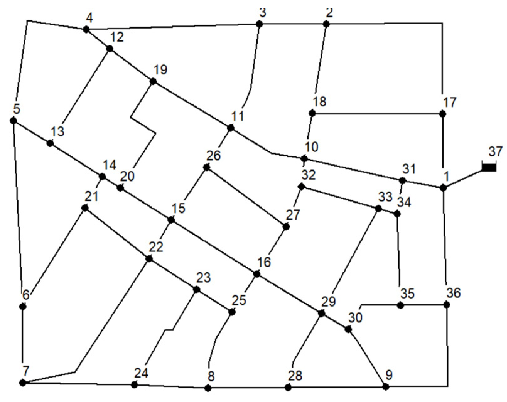
The proposed methodology was applied to the benchmark network Fossolo (FOS) [35], which is composed of 58 pipes, 36 demand nodes, and a reservoir (ID37) with a 121 m head (Figure 1). The material of all the pipes is polyethylene, with a Hazen–Williams coefficient of C = 150. Pressure P0, below which no demand is supplied, is set to 15 m at every node, while pressure Pf, above which demand is fully supplied, is set to 50 m.
It is assumed that all users belong to the residential typology and that nodal demand has a gamma-type pdf, whose mean was that used for the sizing of the WDN [35] and then related to peak-hour demand. The parameters of the scaling law are derived from the dataset analyzed by Magini et al. [11] relating to users of the same type and sampled in peak hour, with a sampling interval of 5 min (Table 1).
Given the demand at the i-th node and the corresponding expected value of the single user demand, μ1, and considering the linear dependency between demand and number of users, the latter is calculated in each node through . Table 2 reports the number of users and the mean demand at each node.
3.2. Generation of Water-Demand Scenarios
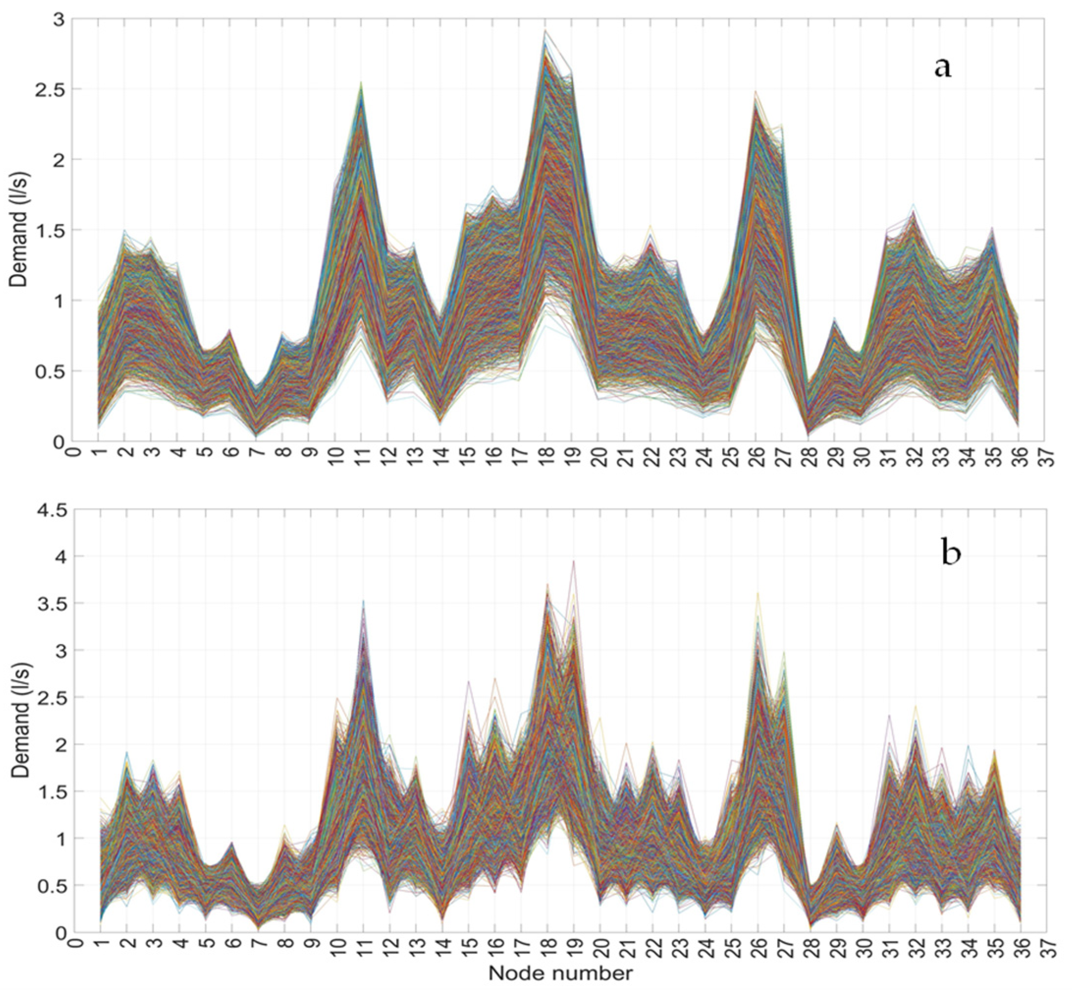
In the first phase of the proposed methodology, a high number of water-demand scenarios are generated based on the statistics estimated through scaling laws, under the hypothesis that, at each node, demand has a gamma-type probability distribution. For the generation of scenarios, a relevant parameter is the correlation between demands at the various nodes. Scaling laws [12] show that this parameter, which is expressed through the Pearson correlation coefficient, depends on the number of users and the mean correlation coefficient between single users, and it increases with the number of aggregated users. The correlation between demands takes a significant role in the analysis of the functioning of a WDN. Filion et al. [36] highlighted that the cross-correlation between nodal demands affects the hydraulic performances of these systems and their reliability. In detail, these authors concluded that the cross-correlation between demands significantly affects the standard deviation of nodal pressure. Therefore, it was decided to examine the influence of this parameter on the performances of the ANN, hence generating two different groups of water-demand scenarios that are characterized by different values of demand cross-correlation: the first group consisted of 10,000 strongly correlated scenarios, obtained by setting the value of cross-correlation between unit users to ρ1 = 0.08; the second group consisted of 10,000 weakly correlated scenarios, with ρ1 = 0.0008 cross-correlation. Figure 2 shows the two groups of generated scenarios.
As a result, the mean value of the cross-correlation coefficient for the nodal demands of the first group of scenarios is ρ = 0.45, while for the second group, it is ρ = 0.0009.
3.3. Pressure Heads Scenarios
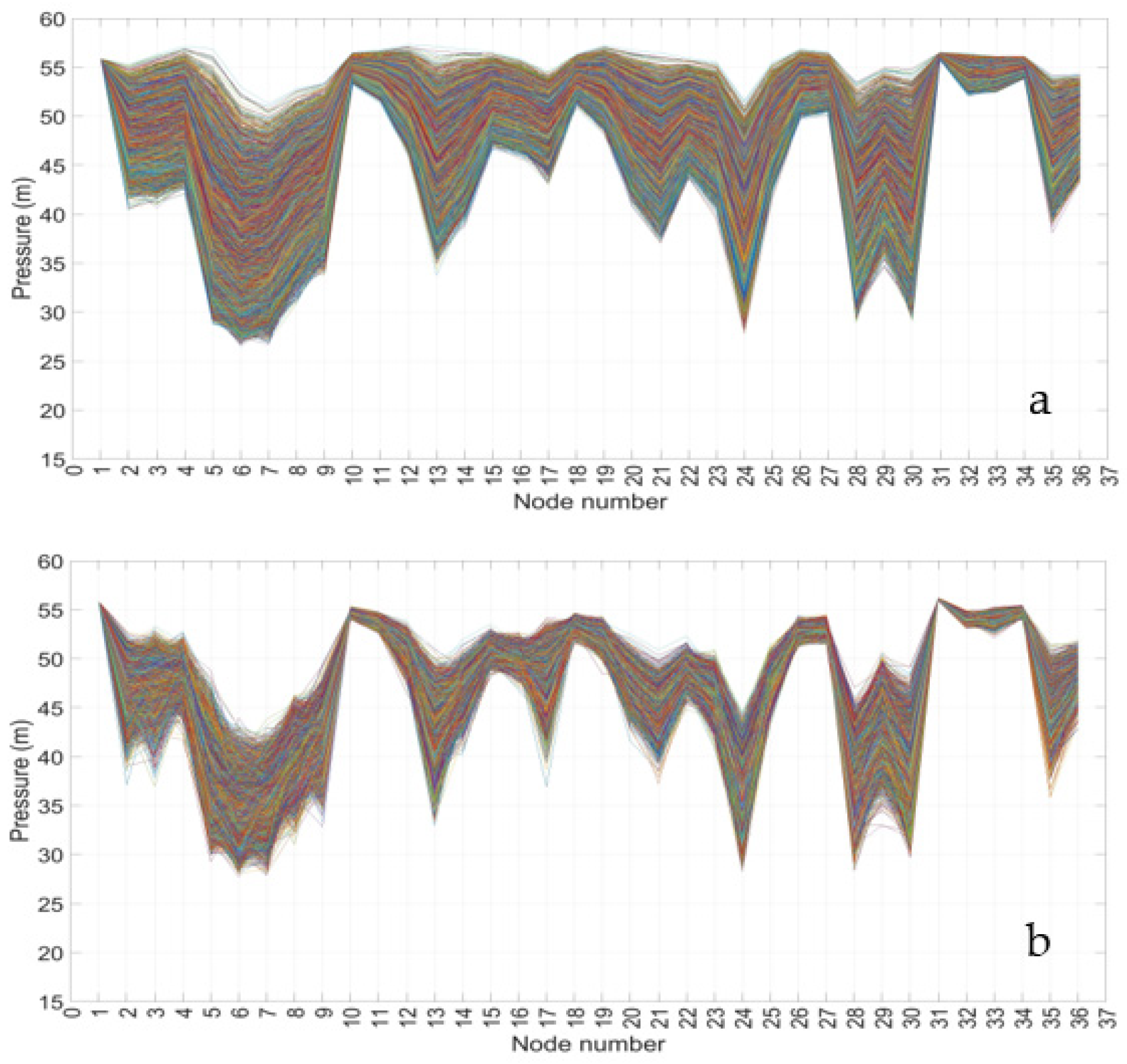
Based on these water-demand scenarios, the corresponding pressure scenarios for the nodes of the WDN were obtained by using the PDA by the hydraulic model Epanet 2.2 [30]. For the 10,000 demand scenarios, the simulations provided, respectively, 8968 and 9372 pressure scenarios that fulfill the service conditions for the two groups, differing by demand cross-correlation. The results are illustrated in Figure 3.
The values of the pressure cross-correlation coefficient are higher for the scenarios corresponding to strongly correlated demands, while they are lower for pressure scenarios obtained from weakly correlated demands. In accordance with the results by Filion et al. [36], the standard deviation of the first group of pressure scenarios (std = 2.6 m) is higher than that of the second group, which is std = 1.4 m.
3.4. Sampling Design for Monitoring the WDN
The goal of this study was the construction of an ANN to estimate the load pressures at each node of the WDN based on the availability of measurements of this parameter in a limited number of nodes. The preliminary step for the construction of the ANN is the choice of the number and the locations of the monitoring sensors. This choice must be made with the aim of achieving the maximum amount of information so that the pressure values provided by the ANN are as similar as possible to the real ones. For this reason, the employed method is based on the optimization of the performance index of the ANN. Here, the latter is calculated through the mean square error (MSE). In this respect, a greedy approach was used which reaches the solution of the problem by selecting the optimal location of the monitored nodes by sequential steps starting from one single location up to the fixed maximum number of locations. This algorithm overlooks the fact that the best result might not coincide with the optimal global solution, and hence it might provide only a suboptimal solution. However, the algorithm results in being easily implementable, and it is scarcely burdensome concerning computation times. Specifically, the previously described ANN was used. The training data were represented by the pressures obtained from the simulations with the generated demand scenarios. The SD procedure starts by considering a single monitoring location, which coincides with each demand node. For each node, the performance index of the ANN is evaluated. Then the node with the best performance is selected. Subsequently, further locations are added one by one, selecting the node that provides the best performance. It is hypothesized that the maximum number of monitored locations is 12, which is around 1/3 of the nodes in the network. The procedure is applied 3 times, respectively, considering the ANN as built from (a) the pressures obtained from strongly correlated demand scenarios; (b) the pressures from the weakly correlated demand scenarios; and (c) all the pressure scenarios from the previous cases, randomly mixed.
The IDs of the nodes selected in the three different cases are reported in Table 3, Table 4 and Table 5, respectively.
The results show that the case corresponding to strongly correlated demand scenarios provides, with the same number of locations, the best performance index, i.e., the smallest value of MSE. Moreover, worst performances are associated with weakly correlated demands (Figure 4).
The choice of monitoring locations is different among the three cases, but they share many nodes. In particular, Cases (a) and (b) share 8 locations out of 12, Cases (a) and (c) share 9 locations out of 12, and Cases (b) and (c) share 11 out of 12. However, there are differences in the ranking orders of the greedy selection. It must be noted that, in all three cases, the nodes that were selected first are characterized by higher values of standard deviation and smaller values of the Pearson cross-correlation coefficient for nodal pressure.
3.5. ANN Results
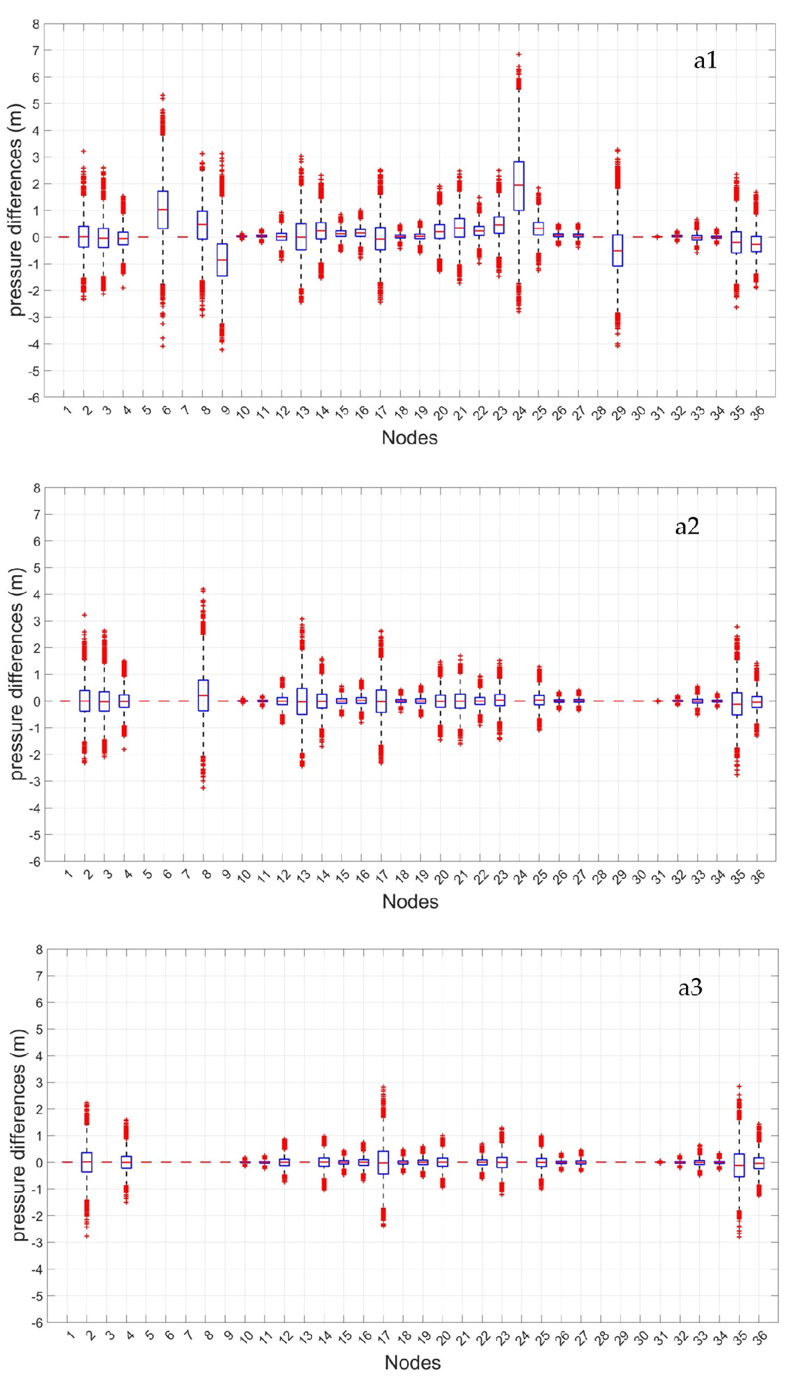
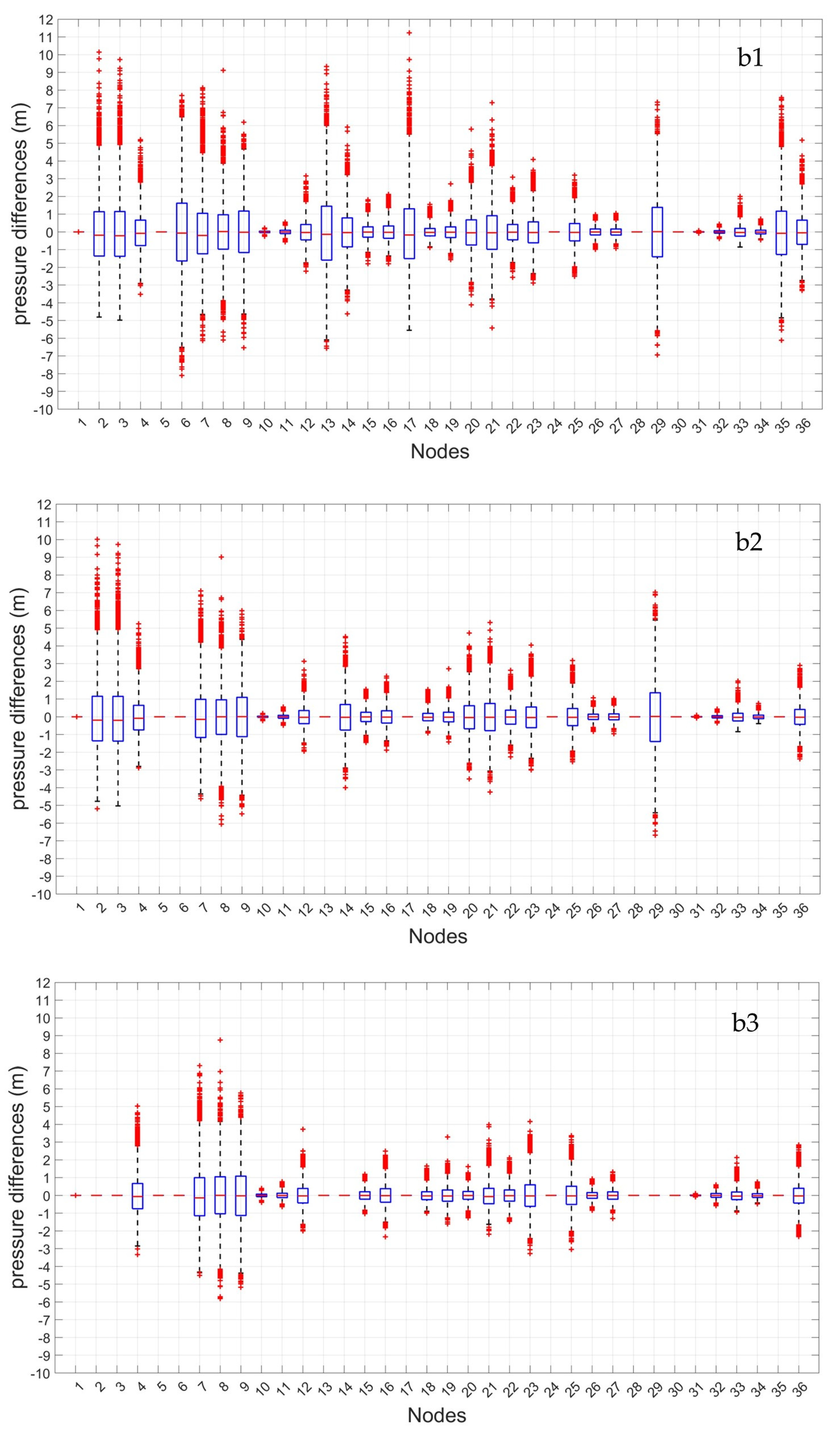
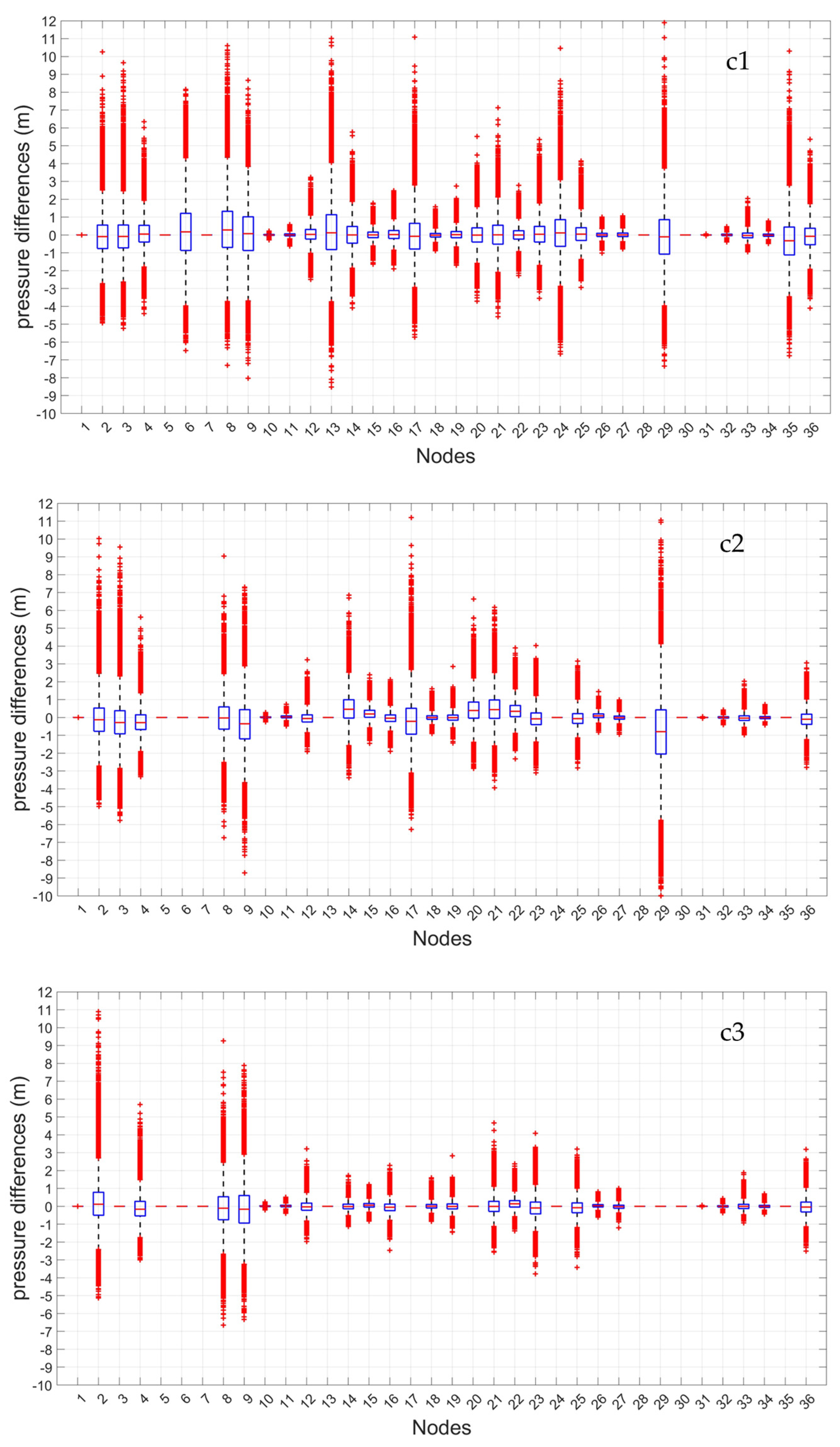
After performing the choice of the number and the position of monitoring locations, the ANN network was used to determine the pressure values at all the nodes of the WDN. Synthetic pressure data were used, generated through the previously described procedure, in the three cases, Cases (a), (b), and (c), related to the different cross-correlation values between water demands. Figure 5, Figure 6 and Figure 7 report the differences between the pressure value estimated by the ANN and the real one for each node, through
The box-plot analysis shows the degree of dispersion of the values of these differences by quartile values. The central box groups 50% of differences. The central red line represents the median (mean quartile); half of the differences are higher or equal to this value, while the other half is lower. If the median is 0, the positive and negative differences between estimated and real pressure values are perfectly balanced. The upper and lower parts of each box represent the sample’s 25th and 75th percentiles. The difference between each box’s lower and upper parts is the interquartile range. The dashed lines above and below each box—the whiskers—stretch from the end of the interquartile range to the most distant value within the whiskers’ length (the adjacent value). Pressure differences beyond the whiskers’ length are marked as outlier values. A value is considered an outlier if its distance from the box’s lower or upper part is higher than 1.5 times the interquartile range and is represented in the following as a red + sign.
The results, which are reported for the cases with 4, 8, and 12 monitoring locations, highlight that, in all three considered cases, the interquartile range and the whiskers’ length decrease significantly with the number of monitoring locations. In particular, in Case (a), with strongly correlated demand scenarios, the maximum interquartile range decreases from around 2 m (Node 24) to less than 1 m (Nodes 2, 17, and 35), respectively, with 4 and 12 monitored nodes. In Case (b), with non-correlated demands, the maximum interquartile range is progressively wider but decreases from 3 m (Nodes 6 and 29) to around 2 m (Nodes 7, 8, and 9), with the increase of monitoring locations. The same result appears in Case (c)—demands with mixed correlation—in which the width of interquartile ranges decreases, and the maximum value is slightly above 2 m (Nodes 6 and 8) for 4 monitoring locations but is lower than 2 m (Node 9) for 12 locations. The whiskers’ length does not significantly change in the three considered cases. In Case (c), there is an increase in the number of outliers, which exceeds 10% of the total in some nodes, while in Cases (a) and (b), it is always lower than 3%. In Cases (b) and (c), the outliers of the differences between estimated and real pressure values are generally quite relevant, also with 12 monitored nodes. The median line tends to coincide with zero in all the nodes of the network as the number of monitoring locations increases.
4. Conclusions
This work employed an artificial neural network to simulate the distribution of water pressure in all the nodes of a WDN, with the availability of pressure values for a limited number of nodes. The ANN was built with synthetic pressure values, which were obtained through a pressure-driven hydraulic model, and demand values for each node, which were randomly sampled from a gamma distribution, with parameters depending on the number of users, derived from the on-field data of residential users. Random sampling was performed by respecting the cross-correlation between nodal demands. The values of the cross-correlation coefficient were also considered as being dependent on the number of served users, being defined as the cross-correlation coefficient for couples of single users. Three different ANNs were examined, each being built with demand scenarios that were differently correlated. The choice of the monitored nodes was performed according to the optimization of the performance parameter of the ANN, as defined by the MSE. The analysis of the results highlighted that the performance of the neural network sensibly improves with the number of monitoring locations in all the considered cases. With the same number of monitored nodes, the performance of the network appears to be strongly influenced by the cross-correlation values between the nodal demands. Markedly better results are produced by strongly correlated scenarios, with a lower width of the interquartile range of the distribution of differences between estimated and real pressure values. In this case, the whiskers in the box-plot representation resulted in being less wide, and the number of outliers was lower. In all three considered cases, for higher numbers of monitoring locations, the null value of the median in the box-plot representation highlights that the statistical centralities of the estimated pressure values and of the real pressure values coincide, confirming that the ANN can perform a significant simulation of the distribution of nodal pressures. The proposed approach turns out to also be useful for the simulation of pressure values bypassing the WDN hydraulic modeling. Future studies will be conducted to verify the influence on the performance of the ANN of the topological structure of the WDN and on the possibility of using more performing machine-learning algorithms.
Author Contributions
Conceptualization, R.M. and R.G.; methodology, R.M. and M.A.B.; software, M.M. and R.M.; validation, M.A.B., M.M. and R.M.; formal analysis, R.M.; investigation, R.M., M.M. and M.A.B.; resources, R.M.; data curation, R.G.; writing—original draft preparation, M.M.; writing—review and editing, R.M.; supervision, R.G.; project administration, R.M.; funding acquisition, R.M. All authors have read and agreed to the published version of the manuscript.
Funding
This research was funded by ‘Sapienza University of Rome’ Progetti di Ricerca (Piccoli, Medi)—Progetti Piccoli, 2020. Protocol number: RP120172B8AB55B7.
Informed Consent Statement
Not applicable.
Data Availability Statement
Water demand data cannot be shared.
Conflicts of Interest
The authors declare no conflict of interest.
References
- Lambert, A.O.; Fantozzi, M. Recent Developments in Pressure Management. In Proceedings of the IWA Conference Water Loss 2010, Sao Paulo, Brazil, 6 June 2010. [Google Scholar]
- Vicente, D.J.; Garrote, L.; Sánchez, R.; Santillán, D. Pressure Management in Water Distribution Systems: Current Status, Proposals, and Future Trends. J. Water Resour. Plan. Manag. 2016, 142, 04015061. [Google Scholar] [CrossRef]
- Di Mauro, A.; Cominola, A.; Castelletti, A.; Di Nardo, A. Urban Water Consumption at Multiple Spatial and Temporal Scales. A Review of Existing Datasets. Water 2020, 13, 36. [Google Scholar] [CrossRef]
- Bruce Billings, R.; Jones, C.V. Forecasting Urban Water Demand; American Water Works Association: Denver, CO, USA, 2011; ISBN 9781613000700. [Google Scholar]
- Maier, H.R.; Guillaume, J.H.A.; van Delden, H.; Riddell, G.A.; Haasnoot, M.; Kwakkel, J.H. An Uncertain Future, Deep Uncertainty, Scenarios, Robustness and Adaptation: How Do They Fit Together? Environ. Model. Softw. 2016, 81, 154–164. [Google Scholar] [CrossRef]
- Buchberger, S.G.; Wu, L. Model for Instantaneous Residential Water Demands. J. Hydraul. Eng. 1995, 121, 232–246. [Google Scholar] [CrossRef]
- Guercio, R.; Magini, R.; Pallavicini, I. Instantaneous Residential Water Demand as Stochastic Point Process. WIT Trans. Ecol. Environ. 2001, 48, 1–10. [Google Scholar] [CrossRef]
- Alvisi, S.; Franchini, M.; Marinelli, A. A Stochastic Model for Representing Drinking Water Demand at Residential Level. Water Resour. Manag. 2003, 17, 197–222. [Google Scholar] [CrossRef]
- Arandia-Perez, E.; Uber, J.G.; Boccelli, D.L.; Janke, R.; Hartman, D.; Lee, Y. Modeling Automatic Meter Reading Water Demands as Nonhomogeneous Point Processes. J. Water Resour. Plan. Manag. 2014, 140, 55–64. [Google Scholar] [CrossRef]
- Blokker, E.J.M.; Vreeburg, J.H.G. Monte Carlo Simulation of Residential Water Demand: A Stochastic End-Use Model. Impacts Glob. Clim. Change 2005, 1–12. [Google Scholar] [CrossRef]
- Magini, R.; Pallavicini, I.; Guercio, R. Spatial and Temporal Scaling Properties of Water Demand. J. Water Resour. Plan. Manag. 2008, 134, 276–284. [Google Scholar] [CrossRef]
- Vertommen, I.; Magini, R.; da Conceição Cunha, M. Scaling Water Consumption Statistics. J. Water Resour. Plan. Manag. 2015, 141, 04014072. [Google Scholar] [CrossRef] [Green Version]
- Alvisi, S.; Ansaloni, N.; Franchini, M. Generation of Synthetic Water Demand Time Series at Different Temporal and Spatial Aggregation Levels. Urban Water J. 2014, 11, 297–310. [Google Scholar] [CrossRef]
- Kossieris, P.; Tsoukalas, I.; Makropoulos, C.; Savic, D. Simulating Marginal and Dependence Behaviour of Water Demand Processes at Any Fine Time Scale. Water 2019, 11, 885. [Google Scholar] [CrossRef]
- Creaco, E.; De Paola, F.; Fiorillo, D.; Giugni, M. Bottom-up Generation of Water Demands to Preserve Basic Statistics and Rank Cross-Correlations of Measured Time Series. J. Water Resour. Plan. Manag. 2020, 146, 06019011. [Google Scholar] [CrossRef]
- Magini, R.; Boniforti, M.A.; Guercio, R. Generating Scenarios of Cross-Correlated Demands for Modelling Water Distribution Networks. Water 2019, 11, 493. [Google Scholar] [CrossRef]
- Creaco, E.; Galuppini, G.; Campisano, A.; Franchini, M. Bottom-Up Generation of Peak Demand Scenarios in Water Distribution Networks. Sustain. Sci. Pract. Policy 2020, 13, 31. [Google Scholar] [CrossRef]
- Lingireddy, S.; Brion, G.M. Artificial Neural Networks in Water Supply Engineering; ASCE: Reston, VA, USA, 2005; ISBN 9780784475607. [Google Scholar]
- Ridolfi, E.; Servili, F.; Magini, R.; Napolitano, F.; Russo, F.; Alfonso, L. Artificial Neural Networks and Entropy-Based Methods to Determine Pressure Distribution in Water Distribution Systems. Procedia Eng. 2014, 89, 648–655. [Google Scholar] [CrossRef]
- Dawidowicz, J. Evaluation of a Pressure Head and Pressure Zones in Water Distribution Systems by Artificial Neural Networks. Neural Comput. Appl. 2018, 30, 2531–2538. [Google Scholar] [CrossRef] [PubMed]
- Jang, D.; Park, H.; Choi, G. Estimation of Leakage Ratio Using Principal Component Analysis and Artificial Neural Network in Water Distribution Systems. Sustain. Sci. Pract. Policy 2018, 10, 750. [Google Scholar] [CrossRef]
- Momeni, A.; Piratla, K.R. A Proof-of-Concept Study for Hydraulic Model-Based Leakage Detection in Water Pipelines Using Pressure Monitoring Data. Front. Water 2021, 3, 648622. [Google Scholar] [CrossRef]
- Nazif, S.; Karamouz, M.; Tabesh, M.; Moridi, A. Pressure Management Model for Urban Water Distribution Networks. Water Resour. Manag. 2010, 24, 437–458. [Google Scholar] [CrossRef]
- Walker, W.E.; Harremoës, P.; Rotmans, J.; van der Sluijs, J.P.; van Asselt, M.B.A.; Janssen, P.; Krayer von Krauss, M.P. Defining Uncertainty: A Conceptual Basis for Uncertainty Management in Model-Based Decision Support. Integr. Assess. 2003, 4, 5–17. [Google Scholar] [CrossRef]
- Gargano, R.; Tricarico, C.; Granata, F.; Santopietro, S.; De Marinis, G. Probabilistic Models for the Peak Residential Water Demand. Water 2017, 9, 417. [Google Scholar] [CrossRef]
- McKay, M.D.; Beckman, R.J.; Conover, W.J. A Comparison of Three Methods for Selecting Values of Input Variables in the Analysis of Output from a Computer Code. Technometrics 1979, 21, 239. [Google Scholar]
- Cario, M.C.; Nelson, B.L. Modeling and Generating Random Vectors with Arbitrary Marginal Distributions and Correlation Matrix; Department of Industrial Engineering and Management Science, Northwestern University: Evanston, IL, USA, 1997. [Google Scholar]
- Iman, R.L.; Conover, W.J. A Distribution-Free Approach to Inducing Rank Correlation among Input Variables. Commun. Stat.—Simul. Comput. 1982, 11, 311–334. [Google Scholar] [CrossRef]
- Eliades, D.G.; Kyriakou, M.; Vrachimis, S.; Polycarpou, M.M. EPANET-MATLAB Toolkit: An Open-Source Software for Interfacing EPANET with MATLAB. In Proceedings of the Computer Control for Water Industry (CCWI 2016), Amsterdam, The Netherlands, 7–9 November 2016. [Google Scholar] [CrossRef]
- Rossman, L.A.; Boulos, P.F.; Altman, T. Discrete Volume-element Method for Network Water-quality Models. J. Water Resour. Plan. Manag. 1993, 119, 505–517. [Google Scholar] [CrossRef]
- Todini, E.; Pilati, S. A Gradient Algorithm for the Analysis of Pipe Networks. In Computer Applications in Water Supply; Coulbeck, B., Orr, C.H., Eds.; John Wiley & Sons: London, UK, 1988; pp. 1–20. [Google Scholar]
- Wagner, J.M.; Shamir, U.; Marks, D.H. Water Distribution Reliability: Simulation Methods. J. Water Resour. Plan. Manag. 1988, 114, 253–275. [Google Scholar] [CrossRef]
- MacKay, D.J.C. Bayesian Interpolation. Neural Comput. 1992, 4, 415–447. [Google Scholar] [CrossRef]
- Foresee, F.D.; Dan Foresee, F.; Hagan, M.T. Gauss-Newton Approximation to Bayesian Learning. In Proceedings of the International Conference on Neural Networks (ICNN’97), Houston, TX, USA, 9–12 June 1997. [Google Scholar]
- Bragalli, C.; D’Ambrosio, C.; Lee, J.; Lodi, A.; Toth, P. Optimizing the Design of Water Distribution Networks Using Mathematical Optimization. In Case Studies in Operations Research; Murty, K., Ed.; International Series in Operations Research & Management Science; Springer: New York, NY, USA, 2015; Volume 212. [Google Scholar] [CrossRef]
- Filion, Y.; Adams, B.; Karney, B.W. Cross Correlation of Demands in Water Distribution Network Design. J. Water Resour. Plan. Manag. 2007, 133, 137–144. [Google Scholar] [CrossRef] [Green Version]
Figure 1.
FOS network layout with nodes’ ID.

Figure 2.
Generated water-demand scenarios: (a) strongly correlated scenarios, ρ1 = 0.08; and (b) weakly correlated scenarios, ρ1 = 0.0008.
Figure 2.
Generated water-demand scenarios: (a) strongly correlated scenarios, ρ1 = 0.08; and (b) weakly correlated scenarios, ρ1 = 0.0008.

Figure 3.
Simulated pressure heads with the different water-demand scenarios: (a) strongly correlated scenarios, ρ1 = 0.08; and (b) weakly correlated scenarios, ρ1 = 0.0008.
Figure 3.
Simulated pressure heads with the different water-demand scenarios: (a) strongly correlated scenarios, ρ1 = 0.08; and (b) weakly correlated scenarios, ρ1 = 0.0008.

Figure 4.
Comparison of the MSE indices for the three different pressure scenarios and different number of monitoring locations: Case (a), green bar; Case (b), red bar; and Case (c), blue bar.
Figure 4.
Comparison of the MSE indices for the three different pressure scenarios and different number of monitoring locations: Case (a), green bar; Case (b), red bar; and Case (c), blue bar.

Figure 5.
Case (a), box plots of the differences between the measured pressures and the pressures estimated by the ANN for different number of monitored nodes: (a1) 4 nodes, (a2) 8 nodes, and (a3) 12 nodes.
Figure 5.
Case (a), box plots of the differences between the measured pressures and the pressures estimated by the ANN for different number of monitored nodes: (a1) 4 nodes, (a2) 8 nodes, and (a3) 12 nodes.

Figure 6.
Case (b), box plots of the differences between the measured pressures and the pressures estimated by the ANN for different number of monitored nodes: (b1) 4 nodes, (b2) 8 nodes, and (b3) 12 nodes.
Figure 6.
Case (b), box plots of the differences between the measured pressures and the pressures estimated by the ANN for different number of monitored nodes: (b1) 4 nodes, (b2) 8 nodes, and (b3) 12 nodes.

Figure 7.
Case (c), box plots of the differences between the measured pressures and the pressures estimated by the ANN for different number of monitored nodes: (c1) 4 nodes, (c2) 8 nodes, and (c3) 12 nodes.
Figure 7.
Case (c), box plots of the differences between the measured pressures and the pressures estimated by the ANN for different number of monitored nodes: (c1) 4 nodes, (c2) 8 nodes, and (c3) 12 nodes.


Table 1.
Scaling-law parameters (Magini et al. [11]).
Table 1.
Scaling-law parameters (Magini et al. [11]).
| Statistical Parameter | Value |
|---|---|
| μ1(L/min) | 0.704 |
| σ1(L/min) | 1.01 |
| Scaling-law exponent α | 1.23 |
Table 2.
Number of users and mean demand at each node.
| Node ID | Number of Users | Mean Peak Demand (L/s) | Node ID | Number of Users | Mean Peak Demand (L/s) |
|---|---|---|---|---|---|
| 1 | 126 | 0.49 | 19 | 483 | 1.89 |
| 2 | 267 | 1.04 | 20 | 240 | 0.94 |
| 3 | 261 | 1.02 | 21 | 246 | 0.96 |
| 4 | 210 | 0.82 | 22 | 249 | 0.97 |
| 5 | 162 | 0.63 | 23 | 222 | 0.87 |
| 6 | 204 | 0.80 | 24 | 174 | 0.68 |
| 7 | 69 | 0.27 | 25 | 198 | 0.77 |
| 8 | 150 | 0.59 | 26 | 435 | 1.70 |
| 9 | 141 | 0.55 | 27 | 366 | 1.43 |
| 10 | 285 | 1.11 | 28 | 78 | 0.31 |
Table 3.
Case (a): selected locations for different number of monitoring nodes.
| 4 Nodes | 5 Nodes | 6 Nodes | 7 Nodes | 8 Nodes | 9 Nodes | 10 Nodes | 11 Nodes | 12 Nodes |
|---|---|---|---|---|---|---|---|---|
| 5 | 5 | 5 | 5 | 5 | 5 | 5 | 5 | 5 |
| 7 | 7 | 7 | 7 | 7 | 7 | 7 | 7 | 7 |
| 28 | 28 | 28 | 28 | 28 | 28 | 28 | 28 | 28 |
| 30 | 30 | 30 | 30 | 30 | 30 | 30 | 30 | 30 |
| 6 | 6 | 6 | 6 | 6 | 6 | 6 | 6 | |
| 24 | 24 | 24 | 24 | 24 | 24 | 24 | ||
| 29 | 29 | 29 | 29 | 29 | 29 | |||
| 9 | 9 | 9 | 9 | 9 | ||||
| 13 | 13 | 13 | 13 | |||||
| 8 | 8 | 8 | ||||||
| 21 | 21 | |||||||
| 3 |
Table 4.
Case (b): selected locations for different number of monitoring nodes.
| 4 Nodes | 5 Nodes | 6 Nodes | 7 Nodes | 8 Nodes | 9 Nodes | 10 Nodes | 11 Nodes | 12 Nodes |
|---|---|---|---|---|---|---|---|---|
| 5 | 5 | 5 | 5 | 5 | 5 | 5 | 5 | 5 |
| 28 | 28 | 28 | 28 | 28 | 28 | 28 | 28 | 28 |
| 30 | 30 | 30 | 30 | 30 | 30 | 30 | 30 | 30 |
| 24 | 24 | 24 | 24 | 24 | 24 | 24 | 24 | 24 |
| 6 | 6 | 6 | 6 | 6 | 6 | 6 | 6 | |
| 13 | 13 | 13 | 13 | 13 | 13 | 13 | ||
| 17 | 17 | 17 | 17 | 17 | 17 | |||
| 35 | 35 | 35 | 35 | 35 | ||||
| 3 | 3 | 3 | 3 | |||||
| 29 | 29 | 29 | ||||||
| 2 | 2 | |||||||
| 14 |
Table 5.
Case (c): selected locations for different number of monitoring nodes.
| 4 Nodes | 5 Nodes | 6 Nodes | 7 Nodes | 8 Nodes | 9 Nodes | 10 Nodes | 11 Nodes | 12 Nodes |
|---|---|---|---|---|---|---|---|---|
| 30 | 30 | 30 | 30 | 30 | 30 | 30 | 30 | 30 |
| 5 | 5 | 5 | 5 | 5 | 5 | 5 | 5 | 5 |
| 28 | 28 | 28 | 28 | 28 | 28 | 28 | 28 | 28 |
| 7 | 7 | 7 | 7 | 7 | 7 | 7 | 7 | 7 |
| 6 | 6 | 6 | 6 | 6 | 6 | 6 | 6 | |
| 13 | 13 | 13 | 13 | 13 | 13 | 13 | ||
| 24 | 24 | 24 | 24 | 24 | 24 | |||
| 35 | 35 | 35 | 35 | 35 | ||||
| 17 | 17 | 17 | 17 | |||||
| 29 | 29 | 29 | ||||||
| 3 | 3 | |||||||
| 20 |
Disclaimer/Publisher’s Note: The statements, opinions and data contained in all publications are solely those of the individual author(s) and contributor(s) and not of MDPI and/or the editor(s). MDPI and/or the editor(s) disclaim responsibility for any injury to people or property resulting from any ideas, methods, instructions or products referred to in the content. |
© 2023 by the authors. Licensee MDPI, Basel, Switzerland. This article is an open access article distributed under the terms and conditions of the Creative Commons Attribution (CC BY) license (https://creativecommons.org/licenses/by/4.0/).
Share and Cite
MDPI and ACS Style
Magini, R.; Moretti, M.; Boniforti, M.A.; Guercio, R. A Machine-Learning Approach for Monitoring Water Distribution Networks (WDNs). Sustainability 2023, 15, 2981. https://doi.org/10.3390/su15042981
AMA Style
Magini R, Moretti M, Boniforti MA, Guercio R. A Machine-Learning Approach for Monitoring Water Distribution Networks (WDNs). Sustainability. 2023; 15(4):2981. https://doi.org/10.3390/su15042981
Chicago/Turabian StyleMagini, Roberto, Manuela Moretti, Maria Antonietta Boniforti, and Roberto Guercio. 2023. "A Machine-Learning Approach for Monitoring Water Distribution Networks (WDNs)" Sustainability 15, no. 4: 2981. https://doi.org/10.3390/su15042981
Note that from the first issue of 2016, this journal uses article numbers instead of page numbers. See further details here.