Potassium Simulation Using HYDRUS-1D with Satellite-Derived Meteorological Data under Boro Rice Cultivation

Abstract

Potassium (K) is a critical nutrient for crops, as it is a major constituent in fertilizer formulations. With increasing concentrations of K in agricultural soil, it is necessary to understand its movement and retention in the soil. Sub-surface modeling is an alternative method to overcome the exhausting and uneconomical methods to study and determine the actual concentration of K in soil. HYDRUS-1D is considered an effective finite-element model which is suitable for sub-surface modeling. This model requires the input of ground-station meteorological (GM) data taken at a daily timestep for the simulation period. It can be a limiting factor in the absence of ground stations. The study compares K predictions in surface and sub-surface soil layers under Boro rice cultivation obtained with the usage of different meteorological datasets. Thus, the main hypothesis of the study was to validate that, in the absence of GM data, satellite-based meteorological data could be utilized for simulating the K concentration in soil. The two meteorological datasets that are considered in the study included the GM and satellite-derived NASA-Power (NP) meteorological datasets. The usage of a satellite meteorological product at a field scale may help in applying the method to other regions where GM data is not available. The numerical model results were validated with field experiments from four experimental fields which included varied K doses. The concentration in soil was assessed at the regular depths (0–5, 5–10, 10–15, 15–30, 30–45 and 45–60 cm), and at various stages of crop growth, from bare soil and sowing, to the tillering stages. The concentration of K was measured in the laboratory and also simulated through the optimized model. The modeled values were compared with measured values statistically using relative root mean square error (RMSER) and Nash–Sutcliffe modeling efficiency (E) for simulating K concentration in the soil for the Boro rice cropping pattern with both GM data and NP data. The model was found most suitable for the 0–30 cm depth on all days and for all treatment variations.

1. Introduction

The semi-arid ecosystem of India is considered significant in terms of both spatial coverage and fertilizers usage. Encompassing the five agro-ecological zones (AEZs 4–8), it absorbed 7.4 million tons of fertilizer (NPK) in the years 2003/04; thus, 47.3% of total fertilizer consumption was utilized for 42.4% of the total gross cropped area (GCA). In terms of fertilizer loading, the per-ha consumption of fertilizer was found, in 2003–2004, to be approximately 100.2 kg (http://www.fao.org/3/a0257e/A0257E05.html, accessed on 28 December 2022). India is considered to have the largest land area (about 44 million ha) occupied by rice cultivation, which contributes approximately 21% of global rice production [1]. About two billion people in Asia are considered to draw 61–70% of their energy requirements from rice and its derivative by-products (FAOSTAT Database, 2014). Rice cultivation at such a large scale consumes a substantial proportion of fertilizer in India, making paddy fields one of the biggest contributors to pollution (non-point source). The basic perception of nutrient/fertilizer modification as well as transportation to paddy fields is insubstantial because of multipart exchanges between the water, soil, and biomass [2]. This multi-part exchange of nutrients mostly results in less intake of nutrients and more leaching. Three processes are the main ways through which Potassium (K) is flushed out from cultivated land: it can be attached to sediment and eroded from the field, it can dissolve in surface water and flow off, or it can dissolute in the soil as leachate and move through the soil profile. In cultivated fields, most of the loss occurs due to erosion, whereas on non-tilled fields most K loss occurs due to dissolution in surface-water runoff or leachate. In the case of BRRI dhan29 (a variety of Boro rice), the optimum concentration of K is suggested to be 80–90 kg ha⁻¹ [3].

The word “Boro” signifies rice cultivation in excess or deposited water after the rainfall both during the Kharif season and in the Rabi season. Boro rice production has increased from nearly 1.35 million ha in 1991 to 2.95 million ha in 2000 [4]. The extension of Boro rice agriculture beyond conventional borders necessitates the rigorous use of agrochemicals. This variety of rice is more profitable for farmers as it grows in the Rabi season after the soil is enriched with water due to previous monsoon rainfall. In real field conditions, continuous cropping methods have resulted in deficiencies in macronutrients such as Phosphorus (P), K, and Sulphur in the soil. Therefore, in continuous cropping, farmers have to rely more and more on agrochemicals to help soil regain its nutrient richness and combat pests to maintain overall productivity [5]. This leads to incorrect use and overdose of fertilizers in the soil. In addition, the applied fertilizer enters the food chain directly or indirectly [6]. This excessive nutrient load (eutrophication) in the water may change the native flora and fauna [7], as well as cause an abundance of algae growth [8,9]. Such an algal bloom can occasionally make the water not only dangerous for human consumption, but also lead to discoloring of the reservoir water [10,11].

Agricultural regimes have to be established to control and regulate the fertilizer quantity in the soil so that the effects of fertilizers on the soil can be scrutinized. For this, predicting subsurface pathways of water [12] and chemicals (nutrients and pesticides) [13] in paddy cultivation are significant for developing specific and proper management practices to control this non-point source of pollution. Sub-surface modeling techniques are well-versed in the simulation of desired variables which makes them an operative, nontime-consuming option. They also provide an alternative to extravagant methods such as field sampling and laboratory experiments for analyzing the concentration of various nutrients that are added to the soil from various sources [14]. Models such as the HYDRA Decision Support System (DSS) [15], Decision support system for agrotechnology transfer (DSSAT) [16], HYDRUS-1D [17], and CropSyst (Cropping Systems Simulation Model) [18] are well-equipped to quantify the subsurface movement of solvents and solutes in soil [19]. HYDRUS-1D has been used previously to simulate soil moisture dynamics within two catchments in the Goulburn River in NSW. The sensitivity analysis in the study found that the soil type and leaf area index were the main factors that were influencing the model performance. Another study focused on the possible utility of HYDRUS-1D in simulating soil wetness conditions at a catchment scale using continuous point-scale soil moisture data (typical of that obtained from permanently installed TDR probes) [20]. HYDRUS-1D has been also utilized to assess water flow and water losses in a direct seeded rice (DSR) field in the Taihu Lake Basin of east China over the course of two seasons with various rainfall and irrigation treatments. The simulations of vertical fluxes were found to be in close agreement with the observations [21]. These studies confirm the model efficiency under various cropping conditions and long durations in the field. Simulation of water balance components (WBCs) is important for sustainable water-resource development and management. Land- and water-resource management can be improved with the understanding of the sub-catchment WBCs, allowing steps to make the system more sustainable [22].

Soil water movement is closely related to solute transport in the soil profile [13,23]. The major limitation in executing these models is that they require real-field initial solute data and soil moisture information along with daily meteorological data. Hence, experimental and theoretical studies may be needed for this purpose. Moreover, studies on fertilizer simulations are not notably included in the Indian marginal farming methods. In addition, the availability of accurate and consistent ground-station meteorological (GM) data constitutes a major limiting factor for determining nutrient availability beneath the surface [24]. To overcome this, the use of satellite-based data can be taken into account. HYDRUS-1D performed well for simulating soil moisture when satellite-based rainfall data has been utilized [25]. Thus, in the current study, NASA-Power (NP) data was used for simulation purposes. This dataset provides not only precipitation but all meteorological parameters, including maximum and minimum temperature, sunshine hours, wind speed and relative humidity. This study is undertaken to understand model simulation with the easily available input parameters, derived from the satellite data in the absence of field data in the unmonitored basins. This makes subsurface models an alternate tool to be used in general crop fields and provides significant aid to precision agriculture. They may also prevent agricultural fields from overdosing K fertilizers by determining their persistence and mobility. A finite-element model for assessing the tenacity of pesticides has already been developed [13]. Hence, developing the understanding of these available models for nutrient studies is the next logical step.

In view of the above, this study aims to determine the tenacity and movement of K using meteorological data under real cropping-field conditions using HYDRUS-1D. It also addresses K simulated concentration in the case of dry direct-seeded Boro rice treated with distinct fertilizer treatment doses and satellite-derived meteorological parameters, to overcome the limitation of the model’s input of the daily field meteorological datasets.

2. Materials and Methodology

2.1. Study Area and Treatment Design

The selected experimental field is situated at an altitude of 81m in the Agricultural Farm of BHU (Latitude 25.256° and Longitude 82.993°) Varanasi, Uttar Pradesh, India. The study utilized, in total, four randomly selected identical experimental plots of 4 m × 4 m size. Selected four plots were hydraulically separated by impervious walls with a thickness of 12 cm across and which reached more than 170 cm, vertically, underground. The climate of the eastern region of the U.P. is generally humid–subtropical, including the dry winters. The variety of the Boro rice found here was Malviya Hu105. The first dose of essential fertilizer was incorporated after the plowing was performed manually, followed by levelling off the field and, eventually, line sowing of the rice seed. The Muriate of Potash was considered a source of K, which was procured locally (and is used by village farmers). The treatments, given in

Table 1. Variations in fertilizer treatments with their respective source.

SI No.	Treatment Name	Details of Treatment	Fertilizer Source for K
1	V1	100% Optimum dose of Fertilizer NPK	Muriate of Potash (K)
2	V2	75% Optimum dose of Fertilizer NPK
3	V3	50% Optimum dose of Fertilizer NPK
4	V4	25% Optimum dose of Fertilizer NPK

, show the percentage of the dose that were applied in the four experimental plots. K was incorporated only once, during the initial split of the fertilizer administration.

2.2. Soil Sample Collection and Analysis

The soil sampling was performed in each plot during four growth stages (bare land (22 February 2018), germination (30 March 2018), seedling emergence (23 May 2018) and late vegetative stage (2 August 2018)). The first sampling date represents the day before sowing, which is 0 days after application (DAA) of seeds. The rest of sampling dates were 34, 86 and 158 DAA. Soil samples at each date were taken at the depths 0–5, 5–10, 10–15, 15–30, 30–45, and 45–60 cm. Soil samples from each layer were collected from three points in the same plot, to make a compound sample. Collected samples were immediately placed in Ziploc bags and were stored under refrigerated conditions until the analysis was carried out. The early concentration of K in the collected samples was measured before the administration of the fertilizer for all the selected plots. In total, 120 samples were collected over the span of this study. The ground-station data for meteorological parameters (daily basis) such as precipitation, mean temperature, sunshine hour, and wind speed, etc., were noted. This dataset was recorded each day over the entire study period.

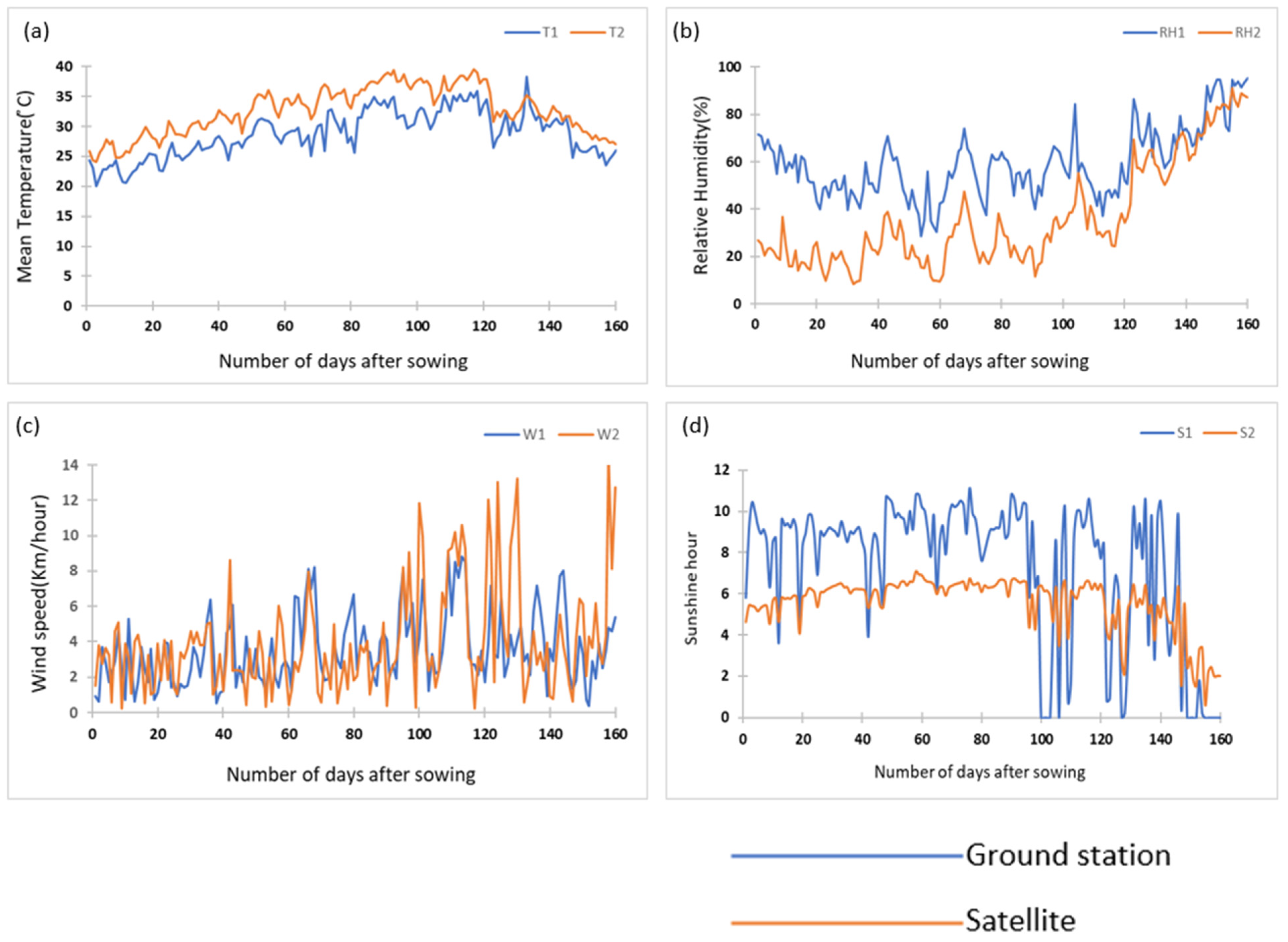
2.3. Collection of Satellite Data

Model simulation needs the precise information of weather datasets and, as the Earth science program initiated by NASA is known for supporting satellite-based research, the weather data obtained from NASA’s Prediction Worldwide Energy Resource (‘POWER’) project was incorporated. This project started in the year 2003 and aimed to facilitate the availability of significant parameters for surface meteorology and solar energy, sustainable buildings, and agro-climatic industries.

The satellite, ground observations, modeling, wind sondes for measuring wind speed and direction, and data assimilation techniques were used to develop the NASA-Power data. The two meteorological datasets used in this study came from the Goddard Earth Observing System Model, version 5.12.4 (GEOS) assimilation model, and the NASA Modern-Era Retro-analysis for Research and Applications (MERRA-2) assimilation model. In order to support NASA’s Earth science research in data analysis, climate and weather prediction, and basic research, the GMAO (Global Modeling and Assimilation Office) is developing the GEOS system of models, which integrates models using the Earth System Modeling Framework (ESMF). The meteorological variables were collected from the POWER website at NASA (https://power.larc.nasa.gov, accessed on 28 December 2022). From the catalogue, one may select the data’s duration and the downloading format of the requested data.

The updated and latest release of POWER 8 is based on Goddard’s Global Modelling and Assimilation Office (GMAO). Primary data sources of solar and meteorological parameters are released on a global grid of 1° × 1° latitude and longitude and are remapped to a 0.5° × 0.5° latitude–longitude using a bilinear interpolation technique. Numerous studies performed in different sub-continents have reported the reliability and accuracy of NP data [26]. The utilized datasets have proven to be accurate for simulations [24]. The methodology adopted to satisfy the present study objectives is shown in Figure 1.

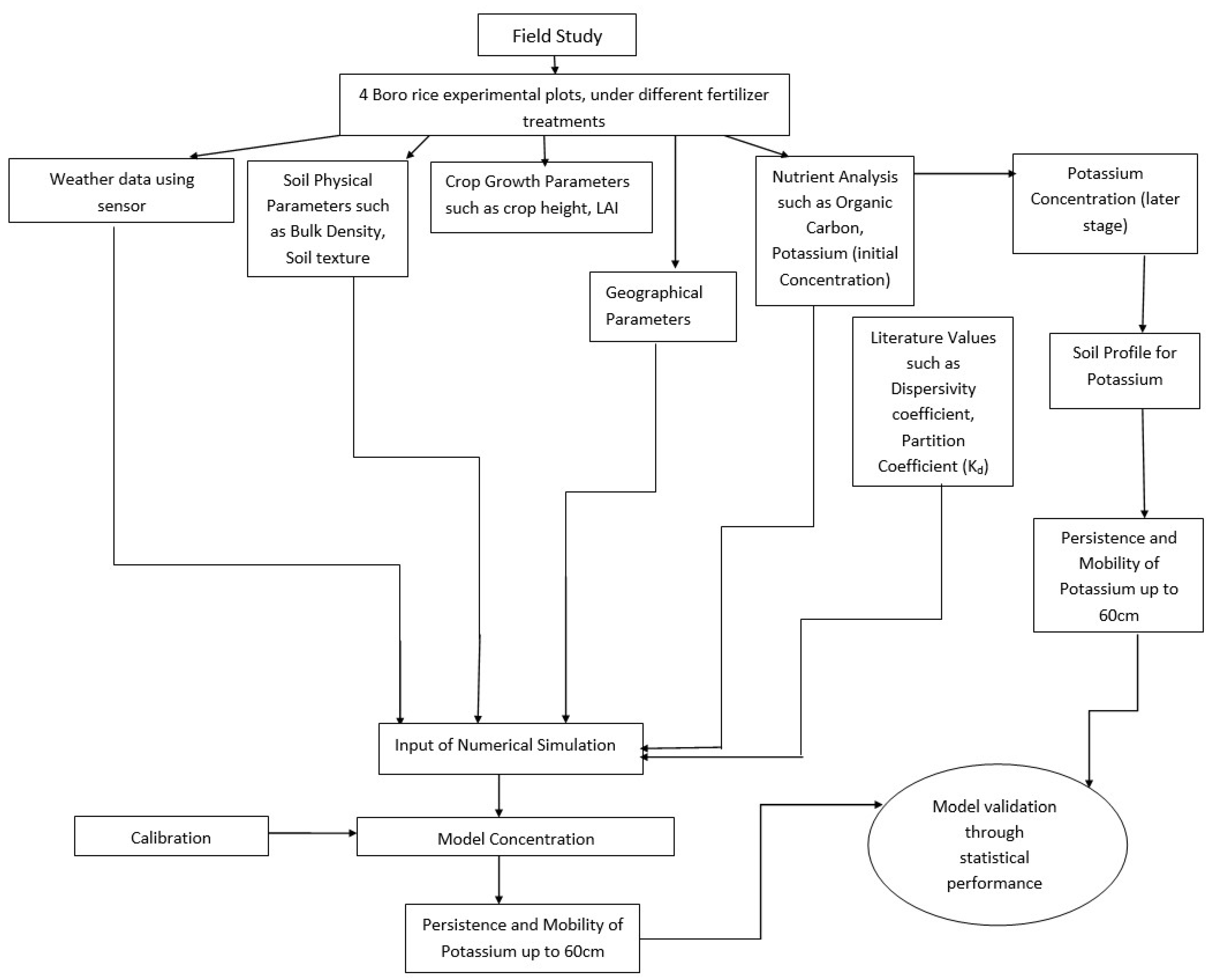
2.4. Numerical Simulation

The transportation of K for Boro rice was simulated numerically utilizing HYDRUS-1D [27]. HYDRUS-1D [28] is a 1-dimensional numerical model for predicting water flow and solute transport in variably saturated porous media. Water flow can be simulated using Richard’s equation. The hydraulic parameters required for the water flow can include a broad range of leading equations, including van Genuchten–Mualem, Brooks–Corey, and Kosugi equations. These equations account for macropore flow using mobile-immobile dual-porosity equations and they can estimate subsurface tile drainage using either the Hooghoudt equation or the Ernest equation [29]. HYDRUS-1D has an adaptable solute transport module, meaning it can simulate a general solute with its adsorption, transport, and reactions, as well as simulate major ions such as CO₂, Ca, Mg, Na, K, SO₄, Cl, NO₃, and H₄SiO₄ [29]. Other activities carried out using the HYDRUS-1D model incorporate heat transport, bacterial transport, 2-site adsorption, and inverse solution of the problems. The details of the governing equations along with input data have been explicitly explained in another study [5] and are not included here, for brevity. The model can be downloaded at no cost from the following link (https://www.pc-progress.com/en/Default.aspx?Downloads, accessed on 28 December 2022).

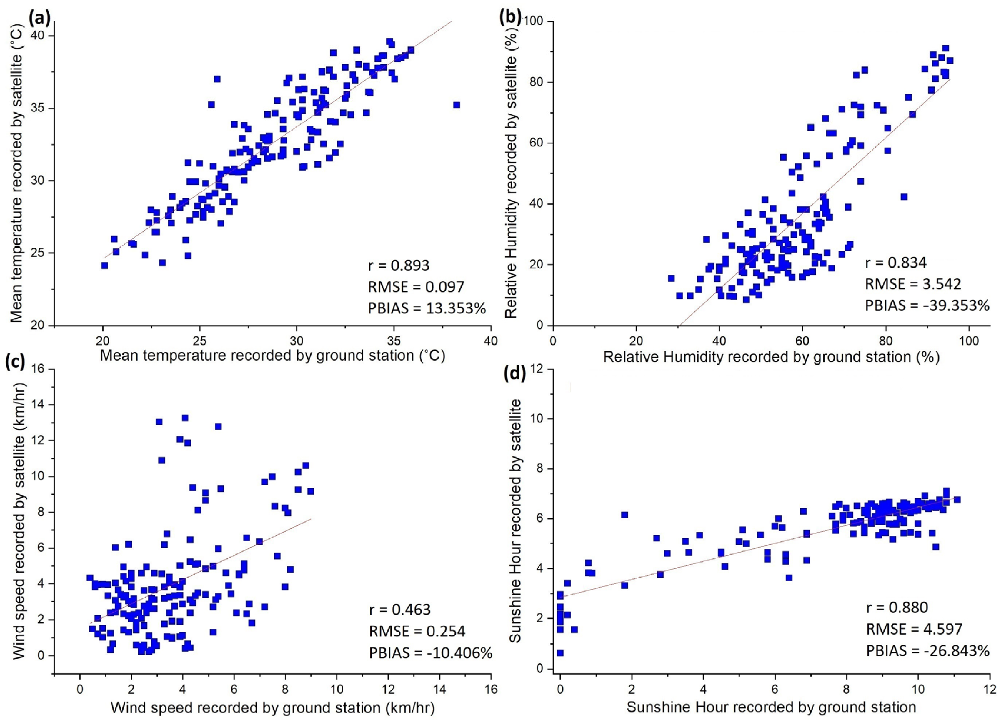
2.5. Statistical Performance

The statistical tools percentage bias (PBIAS), Relative root mean square error (RMSER), and Nash–Sutcliffe modeling efficiency (E) [30,31] were utilized in assessing the agreement between the predicted and observed K concentrations.

RMSER can be defined as

$$\mathrm{RMSER}=\frac{\sqrt{MSE}}{\overline{M}}$$

(1)

$$MSE=\frac{1}{n}{\displaystyle \sum }_{i=1}^n{\left(M-S\right)}^2$$

(2)

where MSE is the mean square error, $\overline{M}$ is the mean value of measured data, M stands for observed K concentration, S stands for simulated K concentration values analogous to the measured value, and n is the total number of the data points. The lower the values of RMSER, the stronger the agreement between simulated values and observed values. E is a measure of the divergence of simulated values from observed values.

$$\mathrm{E}=1-\frac{{{\displaystyle \sum }}_{i=1}^n{(M-S)}^2}{{{\displaystyle \sum }}_{i=1}^n(M-{\overline{M)}}^2}$$

(3)

E can vary between −∞ and 1, where E = 1 indicates an exact match of predicted and measured data values. A negative value indicates that the use of simulated values can increase the chances of divergence from the observed values compared to using the mean observation values. E = 0 specifies that the predictions suggested by the model are nearer to the mean of the observed dataset.

3. Results and Discussion

3.1. Consistency of NP Data

In Figure 2a, the temporal variations in NP derived mean temperature and ground-station-measured temperature clearly show that the satellite sensor captures the correct trend and magnitude of the parameter, even with a grid size of 1° × 1° latitude–longitude. The radiation data was recorded at approx. 111 km and the meteorological data was recorded at 89 km above ground, as per the NP specifications. Although most of the parameters obtained from the satellite are overestimated a little throughout the season, the correlation was highly significant. Figure 2b shows the temporal data of the relative humidity (RH). Satellite-based relative humidity (RH2) is underestimated throughout the season, as compared to RH1. The station-based measurements are near to the ground and as nearness to the ground increases moisture in the air is higher, which makes it more humid. Although precipitation and irrigation contribute to the moisture near the surface, which is not well-captured by the satellite sensor, NP data correctly captures the variation in the trend of RH with a highly significant correlation. The temporal graph of the wind speed (Figure 2c) between the NP and GM data shows high wind speeds were recorded by the satellite throughout the cropping season.

Major episodic patterns in wind speed were also seen between 100 to 138 days, which were not experienced in the vicinity of the planted crops. The wind-speed data were not in agreement with the trend of the ground-station wind-speed data. This discrepancy in data was also consistent with less significant correlation values for the wind speed parameter. Figure 2d displays the temporal variation in the sunshine hours. Ground-station-measured sunshine hours (S1) was consistently high till 100 days of crop plantation, after which it abruptly drops and spikes. This may be attributed to the rainy season and the cloudy sky. The overall reduction in sunshine is also followed by an increase in RH and a decrease in sunshine hours. Sunshine hours from the satellite data is consistently underestimated, which may be attributed to clouds encountered by the sensor at the vertical height of 111 km (as per the NP specifications). Therefore, the number of sunshine hours was also consistent throughout the cropping season, which was not experienced near the ground surface.

The accuracy and reliability of satellite data can be understood through graphical (Figure 2) and statistical analysis, as conducted with the ground measurements. The values of computed correlation coefficient (r) are given in Figure 3. For all the meteorological parameters, a positive and strong correlation is seen between ground-measured and satellite-based data. The linear relationship obtained between mean temperature and ground-station temperature shows the correlation was 0.893 with the lowest root mean square error (RMSE) of 0.097 °C and percentage bias (PBIAS) of 13.353%. This is considered good, according to the range. Relative humidity shows a correlation of 0.834 with ground-station data along with an RMSE of 3.542% and PBIAS value of −39.313%. As explained previously, the vertical distance between the satellite sensor and the crop is high, the satellite cannot account for humidity contributed by moisture present on the ground due to the high vertical distance between the ground and the satellite sensor. Even though a parameter such as wind speed shows a correlation of 0.463 with its ground-measured data, it has a low RMSE value of 0.254 km h⁻¹ and PBIAS of −10.406%, which fall into the criteria of very good in terms of the statistical performance of the data. A close cluster of data points was observed in the case of mean temperature and the most randomness was found for wind speed. The difference in wind-speed data points is due to the vertical height of the sensor from the ground and the obstacles encountered by the wind on the ground, which may contribute to atmospheric disturbances such as cloud cover. In the case of sunshine hours, the correlation was observed to be 0.880 with an RMSE of 4.597 h and PBIAS of −26.843%, which is satisfactory as per the statistical standard. As mentioned above, the radiation data was recorded at 111 km above ground, which is well above the height of cloud cover in the tropics (3–8 km); therefore, the data was nearly consistent throughout the season while ground-station sunshine-hour data varied with the season. Hence, scattered values were obtained across the trendline for the GM data. However, all these linear relationships between NP’s weather datasets and GM data suggested that NP datasets can be used for nutrient simulation in the case of the unavailability of ground-station measurements.

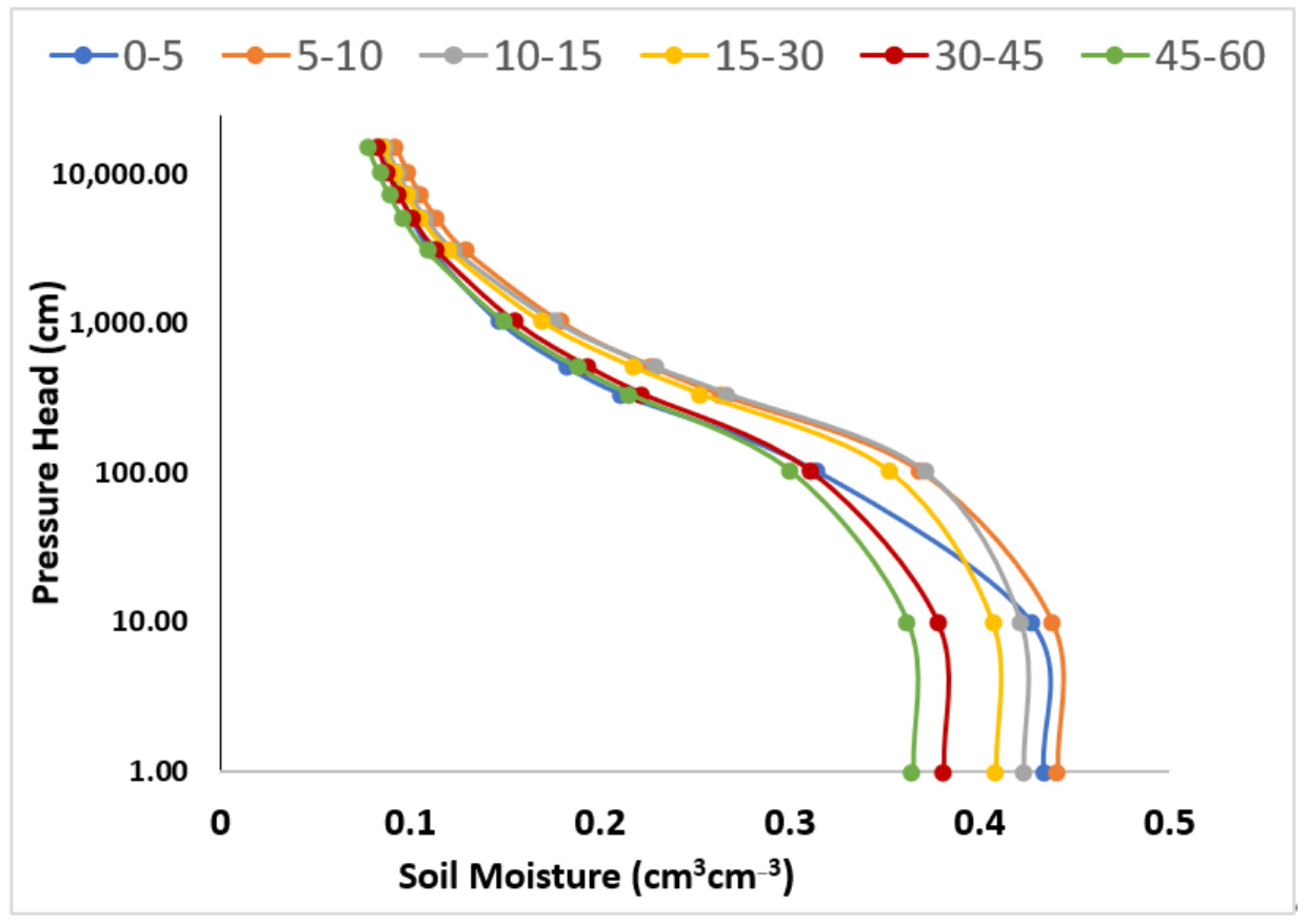
3.2. Model Parametrization and Establishment

HYDRUS-1D is used for the optimization of soil hydraulic parameters [32]. Site-specific irrigation scheduling using one-layer soil hydraulic properties [33,34] and inverse modeling has been performed successfully on palm crops [35] using the model. For these reasons, the HYDRUS-1D was selected to test its efficiency with different fertilizer treatments in multi-soil layer. Several coefficients’ values were selected from various pieces of the literature and the ranges were changed as per the soil conditions and designated climate. The analysis for sensitivity was carried out to test the parameters whose minimum change in input would have a maximum effect on the output. To identify the most sensitive parameter, the predicted fluctuations in the dual-porosity coefficients provided previously [36] were made to alter one at a time. The conventional literature contained the combination of modifying these variables attained within the range. The most sensitive measure, root active uptake, was found to be 0.01 following calibration. The absorption of solute in water is decided by the Michaelis–Menten constant as it is observed to fluctuate within the ranges of 0.5 to 0.0062 and the minimum concentration varied between 0.1 to 0.0023, respectively [37]. The coefficient of the partition [38] varied in the range of 5 to 8 for K. The immobile water concentration varied between 0.01 and 1.01 and the selected range was 0.05–1.01. The calibration process for the coefficient was carried out only for treatment V1 (fertilizer treatment dose was kept optimum as per the International Rice Research Institute (IRR)). After the required calibrations of these parameters for V1, the validation process was executed for V2, V3, and V4 by making use of the calibrated parameters.

The built-in Rosetta module in HYDRUS-1D calculates average hydraulic parameters. The models have already been shown to predict these parameters accurately [13], which are presented in

Table 2. Parameters of van Genuchten functions for soil water retention and hydraulic conductivity curves.

Depth (cm)	$\mathit{\theta }$r (cm3 cm−3)	$\mathit{\theta }$s (cm3 cm−3)	$\mathit{\alpha }$ (cm−1)	n	Ks (cm d−1)	l
0–5	0.068 $\pm$ 0.011	0.434 $\pm$ 0.013	0.015 $\pm$ 0.014	1.553 $\pm$ 0.055	22.755 $\pm$ 5.202	0.5
6–10	0.066 $\pm$ 0.012	0.441 $\pm$ 0.012	0.008 $\pm$ 0.002	1.541 $\pm$ 0.048	22.427 $\pm$ 5.895	0.5
11–15	0.065 $\pm$ 0.010	0.423 $\pm$ 0.019	0.006 $\pm$ 0.001	1.609 $\pm$ 0.033	20.112 $\pm$ 4.720	0.5
16–30	0.063 $\pm$ 0.010	0.408 $\pm$ 0.026	0.007 $\pm$ 0.001	1.581 $\pm$ 0.003	18.252 $\pm$ 5.411	0.5
31–45	0.057 $\pm$ 0.014	0.381 $\pm$ 0.022	0.010 $\pm$ 0.001	1.504 $\pm$ 0.024	11.475 $\pm$ 5.421	0.5
46–60	0.053 $\pm$ 0.011	0.365 $\pm$ 0.017	0.009 $\pm$ 0.001	1.504 $\pm$ 0.015	11.232 $\pm$ 4.927	0.5

. The module gives values of $\theta$_r = residual water content, $\theta$_s = saturated water content, α = coefficient related to n, the pore-size-distribution index (–), n = pore-size-distribution index (–), K_s = hydraulic conductivity, and l = pore connectivity, which is usually 0.5. The soil hydraulic properties were used to plot soil water retention curves for each of the soil depths in Figure 4. Since soil moisture content is also important for the diffusion of K, its simulation in HYDRUS-1D using the Richards equation was also compared to the ground-measured soil water content, as shown in Figure 5. The comparison showed agreeable values of RMSER.

3.3. Model Performance at Various Depths and Treatment Design

The treatments in every selected plot were found to rely on the divergence from the optimum dose of fertilizer for K, which is prescribed by IRRI. In India, 60–65 Kg ha⁻¹ of fertilizer is the advised dose for rice production. The depth-wise variation in the concentration of K for treatment V1 is shown in Figure 6a. The model pattern simulated using GM data was very close to the model pattern simulated using NP data for all the days of sampling. The model shows the closest agreement at 34 DAA as RMSER and E were 0.445 g m⁻³ and 0.806 using GM data. The maximum measured concentration was seen at 1 DAA, as per Figure 6a.

Figure 6b shows the depth-wise variation at 75% of the recommended fertilizer dose (V2). The treatment-measured concentration values for K were in good agreement with model data on all days. The results suggest that the model was working well using NP meteorological data. The model shows the best performance at 34 DAA. This was made evident by the model performance statistics RMSER and E which came out as 0.433 g m⁻³ and 0.774, as shown in

Table 3. Statistical evaluation at different sampling days for each plot.

Treatments	Days	RMSER (g m−3) (Simulated Using GM Data)	RMSER (g m−3) (Simulated Using NP Data)	E (Simulated Using GM Data)	E (Simulated Using NP Data)
V1	1	0.738	0.904	0.435	0.344
	34	0.445	0.445	0.806	0.725
	86	7.983	7.992	0.352	0.318
	158	1.008	1.008	0.412	0.334
V2	1	1.014	1.014	0.032	0.052
	34	0.433	0.432	0.774	0.651
	86	1.862	2.088	0.324	0.282
	158	0.861	0.916	0.096	0.187
V3	1	0.278	0.343	0.910	0.852
	34	0.470	0.467	0.747	0.770
	86	0.907	0.965	0.300	0.386
	158	0.797	0.799	0.328	0.362
V4	1	0.459	0.459	0.857	0.816
	34	0.536	0.598	0.602	0.544
	86	0.728	0.767	0.716	0.743
	158	0.584	0.668	0.956	0.904

using GM meteorological data. The overall analysis of this treatment in Figure 6 at all days compared with the overall analysis of other treatments shows that treatment V2 had the least match. It also suggests that the simulated concentration was the least matched at a depth of 45–60 cm using the meteorological data (Table 3). This suggests that the model did not efficiently simulate the concentration at lower depths in the later days of sampling the crop.

Figure 6c shows the depth-wise analysis variation at 50% of the recommended fertilizer dose (V3). The treatment-measured concentration was in good agreement with the model-simulated values. The model value simulated using NP data at 1 DAA was found to be closest to the measured values using RMSER and E values 0.278 g m⁻³ and 0.910, respectively, using GM data. Figure 6d shows a depth-wise analysis variation in treatment with 25% of the recommended fertilizer dose (V4). The RMSER is 0.536 g m⁻³ and E is found to be 0.602 at 34 DAA. The most accurate results were found in the case of treatment V4. These results were found to be quite consistent with another study [39]. In Table 3, high RMSER values can be clearly seen for the treatments V1 and V2 on different days of the cropping season. Good agreement in mathematically simulated data and ground data was found in the V3 treatment.

The overall temporal analysis for the average fertilizer concentration with respect to days is presented in Figure 7. The statistical measured values between the average simulated concentration and measured concentration of K for all the treatments is shown in

Table 4. Statistical evaluation of average concentration on all days of sampling in each designated treatment plot.

SI No.	Treatments	RMSER (g m−3) (Simulated Using GM Data)	RMSER (g m−3) (Simulated Using NP Data)	E (Simulated Using GM Data)	E (Simulated Using NP Data)
1	V1	3.145	2.587	0.501	0.430
2	V2	1.042	1.112	0.306	0.293
3	V3	0.613	0.643	0.571	0.592
4	V4	0.575	0.623	0.782	0.751

. Except for V2, V3 and V4 had an E above 0.5 for both the meteorological datasets with the calibrated input parameters utilized for the treatment V1. The study shows that NP datasets had comparable results as compared to the GM data. Thus, it is emphasized here that small-scale unmonitored areas can also benefit, as the impact of K dose can be predicted. The method is cost-effective, as only initial soil condition information is required. However, the study is also limited by the fact that the solute parameters need to be calibrated before the model could be utilized for the simulation of K concentration in the soil profile. In the absence of these parameters, the study is limited. In addition, the soil hydraulic parameters were based on the in-situ soil texture dataset. Therefore, if the model is applied at a regional scale, then field data collection can be a limitation and other methods may be required to obtain these parameters, such as inverse optimization with satellite-based products, to reduce the dependency on field observations.

4. Conclusions

The study compared the response of two meteorological datasets as input to HYDRUS-1D for simulations of K in the soil profile. This study emphasized the utilization of satellite-based input datasets, which may be helpful for the unmonitored basins. Four plots with variations in fertilizer treatment were set up to determine the tenacity, route, and mobility of K fertilizer (muriate of potash), specifically for rice crops, using the subsurface model. For this, the concentrations of K at each sampling depth were determined physically and also mathematically modeled using the HYDRUS-1D model. The model was found to be efficient for upper depths up to 30 cm. Too-small or too-large concentrations were found to be most unsuitable for the model predictions. The HYDRUS-1D model can use the input of satellite-derived data products for simulation, which was found to be comparable to the ground-derived information. All the input weather parameters were found to be well-synchronized with the reported ground-station values. Most disagreements found between the NP and GM data with respect to sunshine hours may have occurred due to atmospheric disturbances encountered by the satellite’s sensor. This was followed by wind speed, which was constantly overestimated as compared to GM data. The study showed that utilizing the HYDRUS-1D model before fertilizer application may regulate fertilizer amount. Given that traceable amounts of K were found after crop season in the current investigation, numerical simulations using the HYDRUS-1D can aid in forecasting the residual K in the soil after the crop cycle. Even while their transformation and degradation continually reduce the quantity of elements left in the soil, India’s two crop seasons may likely lead to persistence rather than degradation. Such studies may help provide a mechanism to help practice safer dosage and better management of K treatments in soil. Model simulations with satellite weather data can help in modifying fertilizer dose and limiting carry-over effects.

Other studies have pointed out that the GLDAS-2.1 (Global Land Data Assimilation System) reanalysis dataset released by NASA has a better SWC correlation than ERA5-Land (service of European Space Agency) in some arid regions of China. This can be used for the parameter inverse solution of the HYDRUS-1D model [40,41]. These studies show hydrological models are well-equipped to simulate soil hydraulic parameters with satellite-derived input. Hence, this study successfully confirms that in the presence of limited GM data, satellite data can be utilized and simulations can be helpful in taking decisions regarding safe doses of the fertilizers. This is the only way to ensure agricultural sustainability, the control of conventional farming methods and taking these diffuse anthropogenic influences into account. Therefore, utilizing hydrological modeling and satellite data, as performed in the present study, one can inform fertilizer loading and decisions can be made to avoid soil being overfed with fertilizer. Tools such as sub-surface models are not only helpful from an environmental point of view but also helpful from farmers’ economical point of view, as fertilizer costs are increasing constantly. On a large scale, these types of soil and crop models are necessary to achieve sustainability and better agricultural management in the field of sustainable agriculture. In addition, the synergy of Earth observation datasets and the numerical models is the next step to understand the nutrient simulations at regional scale. Future work includes the importance of nutrient simulations at a regional scale to understand their retention at the large scale. In addition, future studies need to consider other satellite-derived parameters such as soil hydraulic parameters, which can be utilized in the absence of the availability of field-based data, and to, further, make the models independent of in-situ datasets.

References

1. CO, A.; Abd El-Latif, K.; Abdullah, R.; Yusoff, M. Rice production and water use efficiency for self-sufficiency in Malaysia: A review. Trends Appl. Sci. Res. 2011, 6, 1127–1140. [Google Scholar]
2. Ernani, P.R.; Dias, J.; Flore, J.A. Annual additions of potassium to the soil increased apple yield in Brazil. Commun. Soil Sci. Plant Anal. 2002, 33, 1291–1304. [Google Scholar] [CrossRef]
3. Islam, A.; Muttaleb, A. Effect of potassium fertilization on yield and potassium nutrition of Boro rice in a wetland ecosystem of Bangladesh. Arch. Agron. Soil Sci. 2016, 62, 1530–1540. [Google Scholar] [CrossRef]
4. Lal, B.; Gautam, P.; Panda, B.; Raja, R. Boro rice: A way to crop intensification in Eastern India. Pop. Kheti 2013, 1, 5–9. [Google Scholar]
5. Gupta, A.; Gupta, M.; Srivastava, P.K.; Sen, A.; Singh, R.K. Subsurface nutrient modelling using finite element model under Boro rice cropping system. Environ. Dev. Sustain. 2021, 23, 11837–11858. [Google Scholar] [CrossRef]
6. Nádasy, E.; Nádasy, M. Some harmful or useful environmental effect of nitrogen fertilisers. Cereal Res. Commun. 2006, 34, 49–52. [Google Scholar]
7. Wimalawansa, S.A.; Wimalawansa, S.J. Agrochemical-related environmental pollution: Effects on human health. Glob. J. Biol. Agric. Health Sci. 2014, 3, 72–83. [Google Scholar]
8. Li, Y.; Cao, W.; Su, C.; Hong, H. Nutrient sources and composition of recent algal blooms and eutrophication in the northern Jiulong River, Southeast China. Mar. Pollut. Bull. 2011, 63, 249–254. [Google Scholar] [CrossRef]
9. Paerl, H.W.; Otten, T.G. Harmful cyanobacterial blooms: Causes, consequences, and controls. Microb. Ecol. 2013, 65, 995–1010. [Google Scholar] [CrossRef]
10. Lewis, W.M., Jr.; Wurtsbaugh, W.A.; Paerl, H.W. Rationale for control of anthropogenic nitrogen and phosphorus to reduce eutrophication of inland waters. Environ. Sci. Technol. 2011, 45, 10300–10305. [Google Scholar] [CrossRef]
11. Heffernan, J.B.; Liebowitz, D.M.; Frazer, T.K.; Evans, J.M.; Cohen, M.J. Algal blooms and the nitrogen-enrichment hypothesis in Florida springs: Evidence, alternatives, and adaptive management. Ecol. Appl. 2010, 20, 816–829. [Google Scholar] [CrossRef] [Green Version]
12. Garg, N.; Gupta, M. Assessment of improved soil hydraulic parameters for soil water content simulation and irrigation scheduling. Irrig. Sci. 2015, 33, 247–264. [Google Scholar] [CrossRef]
13. Gupta, M.; Garg, N.; Srivastava, P.K. Soil water content influence on pesticide persistence and mobility. In Agricultural Water Management; Elsevier: Amsterdam, The Netherlands, 2021; pp. 307–327. [Google Scholar]
14. Kleinman, P.J.; Smith, D.R.; Bolster, C.H.; Easton, Z.M. Phosphorus fate, management, and modeling in artificially drained systems. J. Environ. Qual. 2015, 44, 460–466. [Google Scholar] [CrossRef] [Green Version]
15. Jacucci, G.; Kabat, P.; Verrier, P.; Teixeira, J.; Steduto, P.; Bertanzon, G.; Giannerini, G.; Huygen, J.; Fernando, R.; Hooijer, A. HYDRA: A decision support model for irrigation water management. In Proceedings of the Crop-Water-Simulation Models in Practice; Selected Papers of the 2nd Workshop on Crop-Water-Models held at the occasion of the 15th Congress of the International Commission on Irrigation and Drainage (ICID), Hague, The Netherlands, 30 August–12 September 1993; Wageningen Pers: Wageningen, The Netherlands, 1995; pp. 315–332. [Google Scholar]
16. Heeren, D.M.; Werner, H.D.; Trooien, T.P. Evaluation of irrigation strategies with the DSSAT cropping system model. In Proceedings of the ASABE/CSBE North Central Intersectional Meeting, Saskatoon, SK, Canada, 5–7 October 2006; p. 1. [Google Scholar]
17. Šimůnek, J.; Hopmans, J.W. Modeling compensated root water and nutrient uptake. Ecol. Model. 2009, 220, 505–521. [Google Scholar] [CrossRef]
18. Stockle, C.; Cabelguenne, M.; Debaeke, P. Validation of CropSyst for water management at a site in southwestern France. In Proceedings of the 4th European Society of Agronomy Congress, Wageningen, The Netherlands, 7–11 July 1996. [Google Scholar]
19. Srivastava, P.K.; Suman, S.; Pandey, V.; Gupta, M.; Gupta, A.; Gupta, D.K.; Chaudhary, S.K.; Singh, U. Concepts and methodologies for agricultural water management. In Agricultural Water Management; Elsevier: Amsterdam, The Netherlands, 2021; pp. 1–18. [Google Scholar]
20. Chen, M.; Willgoose, G.R.; Saco, P.M. Spatial prediction of temporal soil moisture dynamics using HYDRUS-1D. Hydrol. Process. 2014, 28, 171–185. [Google Scholar] [CrossRef]
21. Li, Y.; Šimůnek, J.; Jing, L.; Zhang, Z.; Ni, L. Evaluation of water movement and water losses in a direct-seeded-rice field experiment using Hydrus-1D. Agric. Water Manag. 2014, 142, 38–46. [Google Scholar] [CrossRef] [Green Version]
22. Pandi, D.; Kothandaraman, S.; Kuppusamy, M. Simulation of Water Balance Components Using SWAT Model at Sub Catchment Level. Sustainability 2023, 15, 1438. [Google Scholar] [CrossRef]
23. Wang, K.; Zhang, R.; Hiroshi, Y. Characterizing heterogeneous soil water flow and solute transport using information measures. J. Hydrol. 2009, 370, 109–121. [Google Scholar] [CrossRef]
24. White, J.W.; Hoogenboom, G.; Stackhouse, P.W., Jr.; Hoell, J.M. Evaluation of NASA satellite-and assimilation model-derived long-term daily temperature data over the continental US. Agric. For. Meteorol. 2008, 148, 1574–1584. [Google Scholar] [CrossRef] [Green Version]
25. Gupta, M.; Srivastava, P.K.; Islam, T.; Ishak, A.M.B. Evaluation of TRMM rainfall for soil moisture prediction in a subtropical climate. Environ. Earth Sci. 2014, 71, 4421–4431. [Google Scholar] [CrossRef]
26. Duarte, Y.C.; Sentelhas, P.C. NASA/POWER and DailyGridded weather datasets—How good they are for estimating maize yields in Brazil? Int. J. Biometeorol. 2020, 64, 319–329. [Google Scholar] [CrossRef]
27. Šimůnek, J.; van Genuchten, M.T. Modeling nonequilibrium flow and transport processes using HYDRUS. Vadose Zone J. 2008, 7, 782–797. [Google Scholar] [CrossRef] [Green Version]
28. Šimůnek, J.; van Genuchten, M.T.; Šejna, M. Development and applications of the HYDRUS and STANMOD software packages and related codes. Vadose Zone J. 2008, 7, 587–600. [Google Scholar] [CrossRef] [Green Version]
29. Šimůnek, J.; Jarvis, N.J.; Van Genuchten, M.T.; Gärdenäs, A. Review and comparison of models for describing non-equilibrium and preferential flow and transport in the vadose zone. J. Hydrol. 2003, 272, 14–35. [Google Scholar] [CrossRef]
30. Nash, J.E.; Sutcliffe, J.V. River flow forecasting through conceptual models part I—A discussion of principles. J. Hydrol. 1970, 10, 282–290. [Google Scholar] [CrossRef]
31. Mathevet, T.; Michel, C.; Andréassian, V.; Perrin, C. A bounded version of the Nash-Sutcliffe criterion for better model assessment on large sets of basins. IAHS Publ. 2006, 307, 211. [Google Scholar]
32. Simunek, J.; Van Genuchten, M.T.; Sejna, M. The HYDRUS-1D software package for simulating the one-dimensional movement of water, heat, and multiple solutes in variably-saturated media. Univ. Calif.-Riverside Res. Rep. 2005, 3, 1–240. [Google Scholar]
33. Tan, X.; Shao, D.; Liu, H. Simulating soil water regime in lowland paddy fields under different water managements using HYDRUS-1D. Agric. Water Manag. 2014, 132, 69–78. [Google Scholar] [CrossRef]
34. Kumar, H.; Srivastava, P.; Lamba, J.; Diamantopoulos, E.; Ortiz, B.; Morata, G.; Takhellambam, B.; Bondesan, L. Site-specific irrigation scheduling using one-layer soil hydraulic properties and inverse modeling. Agric. Water Manag. 2022, 273, 107877. [Google Scholar] [CrossRef]
35. Abd Rashid, N.S.; Askari, M.; Tanaka, T.; Simunek, J.; van Genuchten, M.T. Inverse estimation of soil hydraulic properties under oil palm trees. Geoderma 2015, 241, 306–312. [Google Scholar] [CrossRef] [Green Version]
36. Haws, N.W.; Rao, P.S.C.; Simunek, J.; Poyer, I.C. Single-porosity and dual-porosity modeling of water flow and solute transport in subsurface-drained fields using effective field-scale parameters. J. Hydrol. 2005, 313, 257–273. [Google Scholar] [CrossRef]
37. Teo, Y.H.; Beyrouty, C.A.; Norman, R.J.; Gbur, E.E. Nutrient uptake relationship to root characteristics of rice. Plant Soil 1995, 171, 297–302. [Google Scholar] [CrossRef]
38. Sikder, M.S. Advancing Precipitation and Transboundary Flood Forecasting in Monsoon Climates. Ph.D. Thesis, University of Washington, Seattle, WA, USA, 2018. [Google Scholar]
39. Behera, S.; Panda, R. Assessing soil and groundwater contamination with HYDRUS-1D: A study from West Bengal. Environ. Qual. Manag. 2011, 20, 59–75. [Google Scholar] [CrossRef]
40. Wu, Z.; Feng, H.; He, H.; Zhou, J.; Zhang, Y. Evaluation of soil moisture climatology and anomaly components derived from ERA5-land and GLDAS-2.1 in China. Water Resour. Manag. 2021, 35, 629–643. [Google Scholar] [CrossRef]
41. Yu, J.; Wu, Y.; Xu, L.; Peng, J.; Chen, G.; Shen, X.; Lan, R.; Zhao, C.; Zhangzhong, L. Evaluating the Hydrus-1D Model Optimized by Remote Sensing Data for Soil Moisture Simulations in the Maize Root Zone. Remote Sens. 2022, 14, 6079. [Google Scholar] [CrossRef]
Figure 1. Workflow of the methodology adopted in the present study.
Sustainability 15 02147 g001
Figure 2. Meteorological parameters obtained from the ground station and satellite-derived product (a) temperature (T), (b) relative humidity, (RH) (c) wind speed, (W) and (d) sunshine hours (S), respectively.
Sustainability 15 02147 g002
Figure 3. Scatter plots of meteorological parameters obtained from the ground station and satellite-derived products (a) temperature (T), (b) relative humidity (RH), (c) wind speed (W), (d) sunshine hours (S), respectively. Note: The root mean square error (RMSE) measured in Figure 3 (a) is in °C, (b) is in %, (c) is in km h, and (d) is in hours.
Sustainability 15 02147 g003
Figure 4. Soil water retention curves for the six soil depths.
Sustainability 15 02147 g004
Figure 5. Measured and simulated soil water content at depths (a) 0–5 cm, (b) 20 cm, and (c) 50 cm using ground-station meteorological (GM) data and NASA-Power (NP) data.
Sustainability 15 02147 g005
Figure 6. Average concentration simulated using GM meteorological data, simulated using NP meteorological data, and lab measured K at 1 DAA (, --, ), at 34 DAA (, --, ), at 86 DAA (, --, ), and at 158 DAA (, --, ) for treatment (a) V1, (b) V2, (c) V3 and (d) V4, respectively.
Sustainability 15 02147 g006
Figure 7. Average concentration simulated using GM meteorological data, simulated using NP meteorological data, and lab measured K for V1 (, --, ), for V2 (, --, ), for V3 (, --, ), and (, --, ) for V4, respectively during whole study period up to 60 cm of depth.
Sustainability 15 02147 g007