
Can Mechanization Promote Green Agricultural Production? An Empirical Analysis of Maize Production in China
Abstract
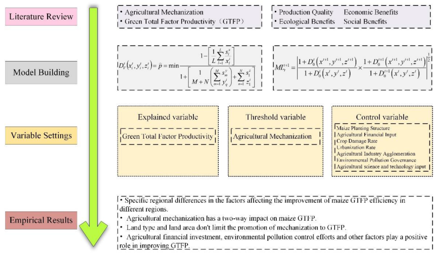
:1. Introduction
2. Literature Review and Mechanism Analysis
2.1. Calculation of Agricultural GTFP
2.2. Influencing Factors of Agricultural GTFP
2.3. Impact of Mechanization on Agricultural GTFP
2.4. Research Assumptions
3. Materials and Methods
3.1. Methods
3.1.1. Super-Efficient SBM
3.1.2. Malmquist–Luenberger Index
3.1.3. Threshold Regression
3.2. Definition of Variables
3.2.1. GTFP Measurement: Input and Output Variables
3.2.2. Influence Factor Variables
3.3. Samples and Data Sources
4. Empirical Results
4.1. Measurement Results of GTFP of Maize
4.1.1. Characteristics of GTFP of Maize
4.1.2. Optimization of GTFP of Maize
4.2. Threshold Effect of Agricultural Mechanization on GTFP of Maize
4.2.1. Stationarity Test
4.2.2. Threshold Effect Test Results
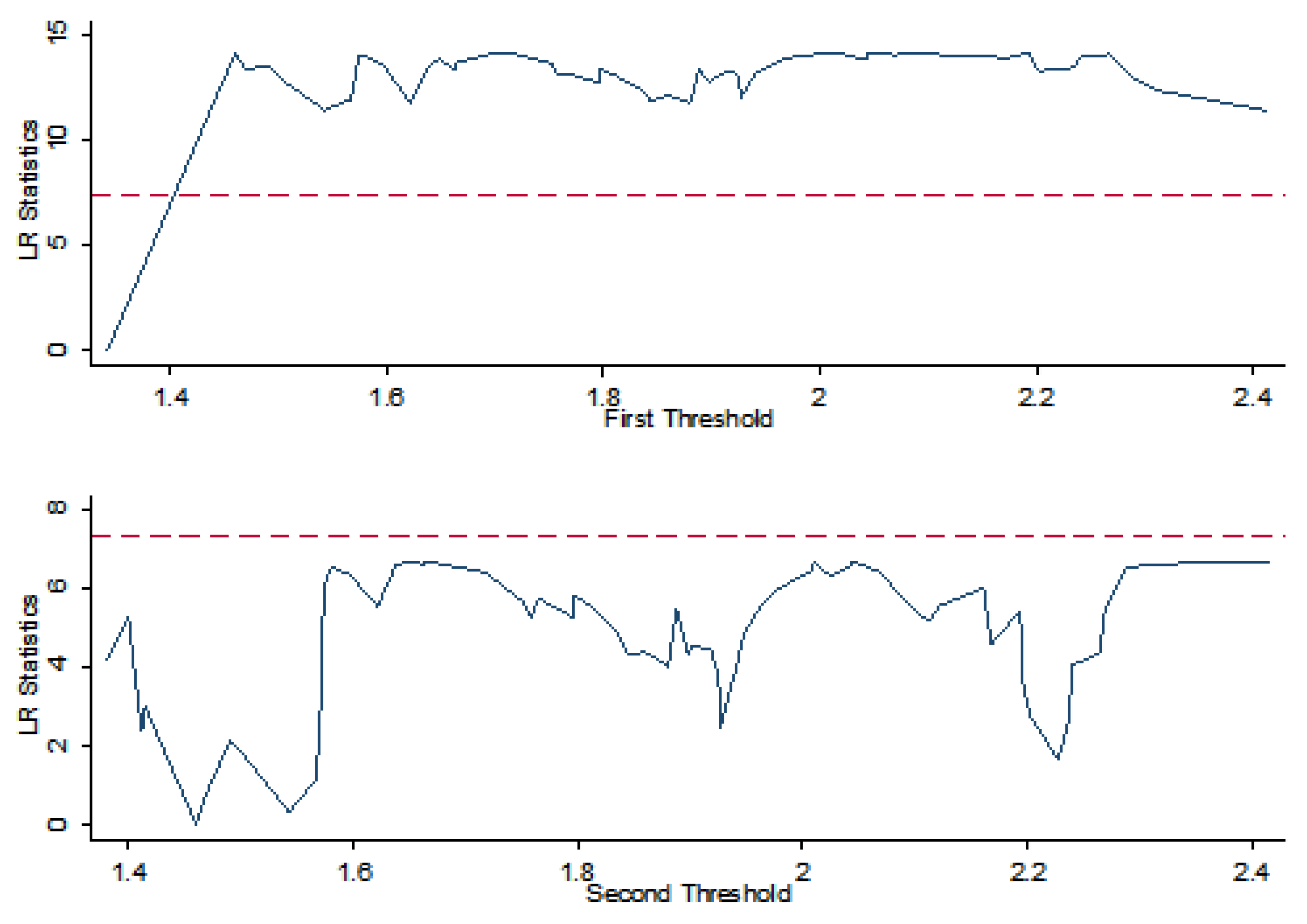
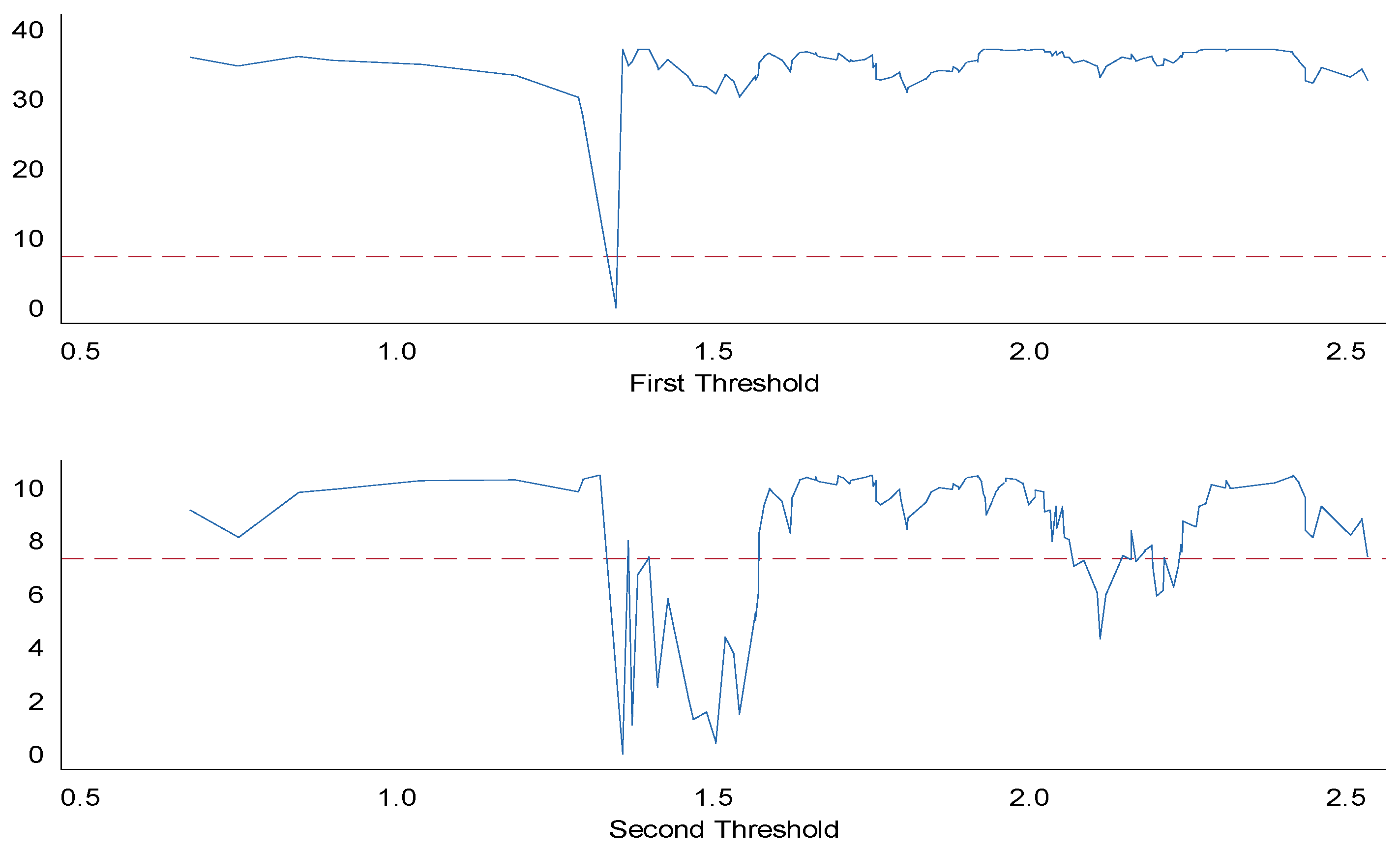
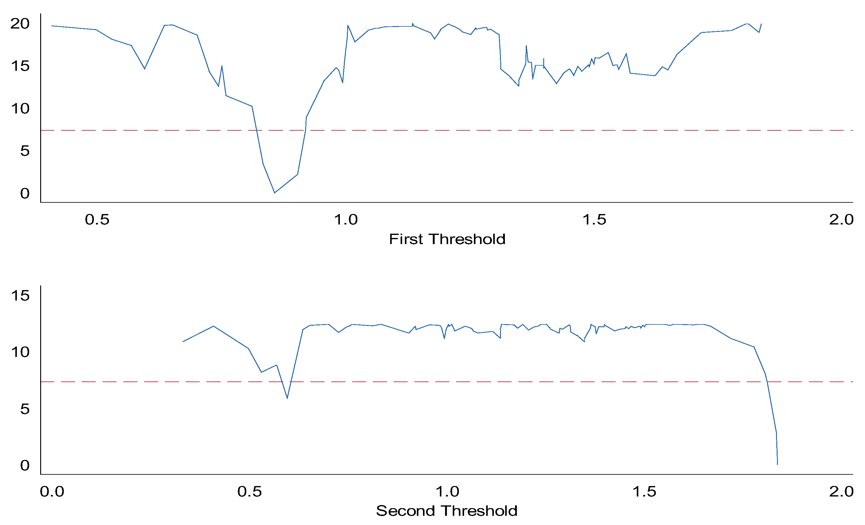
4.2.3. Threshold Estimation Results
4.2.4. Threshold Regression Results
4.2.5. Robustness Test
5. Discussion
6. Conclusions and Implications
6.1. Conclusions
6.2. Policy Implications
6.3. Research Limitations
Author Contributions
Funding
Institutional Review Board Statement
Informed Consent Statement
Data Availability Statement
Conflicts of Interest
Abbreviations
| GTFP | Green Total Factor Productivity |
| SBM-ML | Slack Based Measure-Malmquist-Luenberger |
| MECH | Level of Agricultural Mechanization |
| STRU | Planting Structure of Maize |
| FINA | Agricultural Financial Input |
| DISA | Crop Damage Rate |
| URBA | Urbanization Rate |
| AGGL | Agricultural Industry Agglomeration |
| ENVI | Environmental Pollution Governance |
| SCTE | Agricultural Science and Technology Input |
References
- Johnson, D.G. Agriculture and the wealth of nations. Am. Econ. Rev. 1997, 87, 1–12. [Google Scholar]
- Xia, F.; Xu, J. Green total factor productivity: A re-examination of quality of growth for provinces in China. China Econ. Rev. 2020, 62, 101454. [Google Scholar] [CrossRef]
- Zhou, R.M. Technical progress, technical efficiency, and productivity growth of China’s agriculture. J. Quant. Technol. Econ. 2009, 26, 70–82. [Google Scholar]
- Liu, D.D.; Zhu, X.Y.; Wang, Y.F. China’s agricultural green total factor productivity based on carbon emission: An analysis of evolution and influencing factors. J. Clean. Prod. 2020, 278, 123692. [Google Scholar] [CrossRef]
- Martin, P.L.; Olmstead, L. The Agricultural mechanization controversy. Science 1985, 227, 601–606. [Google Scholar] [CrossRef]
- Rodolfo, T.L. Agricultural mechanization, work and subjectivity: The theory of social representations as a resource for understanding the changes occurred in Brazilian sugarcane fields. Rev. Colomblana Sociol. 2021, 44, 73–96. [Google Scholar]
- Alanoud, A.; Farrukh, N. A review of applications of linear programming to optimize agricultural solutions. Int. J. Inf. Eng. Electron. Bus. 2021, 13, 11–21. [Google Scholar]
- Xue, C.; Shi, X.Y.; Zhou, H. Influence path of agricultural mechanization on total factor productivity growth in planting industry. J. Agrotech. Econ. 2020, 10, 87–102. [Google Scholar]
- Zhang, J.H.; Zheng, F.Y.; Gao, D. The impact of China’s labor transfer on total factor productivity growth. Chin. J. Popul. Sci. 2020, 6, 29–40+126–127. [Google Scholar]
- Lv, N.; Zhu, L.Z. Study on China’s agricultural environmental technical efficiency and green total factor productivity growth. J. Agrotech. Econ. 2019, 4, 95–103. [Google Scholar]
- Deng, H.T.; Cui, B.M. The nature of the property right of the Chinese agricultural land during institution change: The angle of view of the history. Nankai Econ. Stud. 2007, 6, 118–141. [Google Scholar]
- Bentley, J.W. Economic and ecological approaches to land fragmentation: In defense of a Much-Maligned Phenomenon. Annu. Rev. Anthropol. 1987, 16, 31–67. [Google Scholar] [CrossRef]
- Ismael, M.; Srouji, F.; Boutabba, M.A. Agricultural technologies and carbon emissions: Evidence from Jordanian economy. Environ. Sci. Pollut. Res. Int. 2018, 25, 10867–10877. [Google Scholar] [CrossRef] [PubMed]
- Akbar, U.; Li, Q.; Akmal, M.A.; Shakib, M.; Iqbal, W. Nexus between agro-ecological efficiency and carbon emissions transfer: Evidence from China. Environ. Sci. Pollut. Res. Int. 2021, 28, 18995–19007. [Google Scholar] [CrossRef] [PubMed]
- Aigner, D.; Lovell, C.K.; Schmidt, P. Formulation and estimation of stochastic frontier production function models. J. Econom. 1977, 6, 21–37. [Google Scholar] [CrossRef]
- Lin, B.Q.; Wang, X.L. Exploring energy efficiency in China’s iron and steel industry: A stochastic frontier approach. Energy Policy 2014, 72, 87–96. [Google Scholar] [CrossRef]
- Fare, R.; Grosskopf, S.; Norris, M.; Zhang, Z. Productivity growth, technical progress and efficiency change in the industrialised countries. Am. Econ. Rev. 1994, 84, 66–83. [Google Scholar]
- Tugcu, C.T.; Tiwari, A.K. Does renewable and/or non-renewable energy consumption matter for total factor productivity (TFP) growth? Evidence from the BRICS. Renew. Sustain. Energy Rev. 2016, 65, 610–616. [Google Scholar] [CrossRef]
- Wang, X.L.; Sun, C.Z.; Wang, S.; Zhang, Z.; Zou, W. Going green or going away? A spatial empirical examination of the relationship between environmental regulations, biased technological progress, and green total factor productivity. Int. J. Environ. Res. Public Health 2018, 15, 1917. [Google Scholar] [CrossRef]
- Chung, Y.H.; Färe, R.; Grosskopf, S. Productivity and undesirable outputs: A directional distance function approach. J. Environ. Manag. 1997, 51, 229–240. [Google Scholar] [CrossRef] [Green Version]
- Xu, X.C.; Huang, X.Q.; Huang, J.; Gao, X.; Chen, L. Spatial-temporal characteristics of agriculture green total factor productivity in China, 1998–2016: Based on more sophisticated calculations of carbon emissions. Int. J. Environ. Res. Public Health 2019, 16, 3932. [Google Scholar] [CrossRef] [PubMed] [Green Version]
- Chen, Y.F.; Miao, J.F.; Zhu, Z.T. Measuring green total factor productivity of China’s agricultural sector: A three-stage SBM-DEA model with non-point source pollution and CO2 emissions. J. Clean. Prod. 2021, 318, 128543. [Google Scholar] [CrossRef]
- Zhan, J.T.; Tian, X.; Zhang, Y.Y.; Yang, X.; Qu, Z.; Tan, T. The effects of agricultural R&D on Chinese agricultural productivity growth: New evidence of convergence and implications for agricultural R&D policy. Can. J. Agric. Econ. /Rev. Can. 2017, 65, 453–475. [Google Scholar]
- Liu, J.X.; Dong, C.R.; Liu, S.T.; Rahman, S.; Sriboonchitta, S. Sources of total-factor productivity and efficiency changes in China’s agriculture. Agriculture 2020, 10, 279. [Google Scholar] [CrossRef]
- Liu, F.; Lv, N. The threshold effect test of Human capital on the growth of agricultural green total factor productivity: Evidence from China. Int. J. Electr. Eng. Educ. 2021, in press. [Google Scholar] [CrossRef]
- Fang, L.; Hu, R.; Mao, H.; Chen, S.J. How crop insurance influences agricultural green total factor productivity: Evidence from Chinese farmers. J. Clean. Prod. 2021, 321, 128977. [Google Scholar] [CrossRef]
- Gao, F. Evolution trend and internal mechanism of regional total factor productivity in Chinese agriculture. J. Quant. Technol. Econ. 2015, 5, 3–19,53. [Google Scholar]
- Liu, Z. Analysis on the dynamic and influencing factors of agricultural total factor productivity in China. Chin. J. Agric. Resour. Reg. Plan. 2018, 39, 104–111. [Google Scholar]
- Ge, P.F.; Wang, S.J.; Huang, X.L. Measurement for China’s agricultural green TFP. China Popul. Resour. Environ. 2018, 28, 66–74. [Google Scholar]
- Song, M.L.; Li, H. Total factor productivity and the factors of green industry in Shanxi Province, China. Growth Change 2020, 51, 488–504. [Google Scholar] [CrossRef]
- Kajol, R.; Akshay, K.K.; Keerthan, K.T. Automated agricultural field analysis and monitoring system using IOT. Int. J. Inf. Eng. Electron. Bus. 2018, 10, 17–24. [Google Scholar]
- Devkota, R.; Pant, L.P.; Gartaula, H.N.; Patel, K.; Gauchan, D.; Hambly-Odame, H.; Thapa, B.; Raizada, M.N. Responsible agricultural mechanization innovation for the sustainable development of Nepal’s hillside farming system. Sustainability 2020, 12, 374. [Google Scholar] [CrossRef] [Green Version]
- Zhou, X.S.; Ma, W.L. Agricultural mechanization and land productivity in China. Int. J. Sustain. Dev. World Ecol. 2022, 29, 530–542. [Google Scholar] [CrossRef]
- Yukichi, M.; Kazushi, T.; Keijiro, O. Mechanization in land preparation and agricultural intensification: The case of rice farming in the Cote d’Ivoire. Int. J. Sustain. Dev. World Ecol. 2020, 51, 899–908. [Google Scholar]
- Daum, T.; Adegbola, Y.P.; Kamau, G.; Daudu, C.; Zossou, R.C.; Crinot, G.F.; Houssou, P.; Mose, L.; Ndirpaya, Y.; Wahab, A.A.; et al. Perceived effects of farm tractors in four African countries, highlighted by participatory impact diagrams. Agric. Econ. 2020, 40, 47. [Google Scholar] [CrossRef]
- Jaleta, M.; Baudron, F.; Skoko, B.K.; Erenstein, O. Agricultural mechanization and reduced tillage: Antagonism or synergy? Int. J. Agric. Sustain. 2019, 17, 219–230. [Google Scholar] [CrossRef]
- Takeshima, H.; Hatzenbuehler, P.L.; Edeh, H.O. Effects of agricultural mechanization on economies of scope in crop production in Nigeria. J. Dev. Areas 2020, 177, 102691. [Google Scholar] [CrossRef]
- Qiu, T.W.; Boris, C.S.; Biliang, L. Is small beautiful? Links between agricultural mechanization services and the productivity of different-sized farms. Appl. Econ. 2022, 54, 430–442. [Google Scholar] [CrossRef]
- Takeshima, H.; Yanyan, L. Smallholder mechanization induced by yield-enhancing biological technologies: Evidence from Nepal and Ghana. Agric. Syst. 2020, 184, 102914. [Google Scholar] [CrossRef]
- Purba, T.; Helmi, H.; Sembiring, F.; Siagian, D.; Haloho, L.; Girsang, M.; Ramija, K. Measuring the effectiveness of agricultural mechanization performance on irrigated rice area in Batubara Regency. In Proceedings of the 1st International Conference on Sustainable Management and Innovation, ICoSMI 2020, Bogor, West Java, Indonesia, 14–16 September 2020. [Google Scholar]
- Takeshima, H.; Kumar, A. Returns to scale and factor endowments induced specialization: Agricultural mechanization and agricultural transformation in Nepal. J. Dev. Areas 2021, 55, 133–145. [Google Scholar] [CrossRef]
- Haryono, D.; Hudoyo, A.; Mayasari, I. The sustainable agricultural mechanization of rice farming and its impact on land productivity and profit in Lampung Tengah Regency. IOP Conf. Ser. Earth Environ. Sci. 2021, 739, 012056. [Google Scholar] [CrossRef]
- Takeo, M.; Thanh, T.C.; Dung, L.C.; Kitaya, Y.; Maeda, Y. Transition of agricultural mechanization, agricultural economy, government policy and environmental movement related to rice production in the Mekong Delta, Vietnam after 2010. AgriEngineering 2020, 2, 649–675. [Google Scholar]
- Emami, M.; Morteza, A.; Hossein, B.; Kalantari, I. Agricultural mechanization as the driver of reducing food loss and waste in developing countries: Evidence from Iran. Russ. Agric. Sci. 2021, 47, 530–535. [Google Scholar] [CrossRef]
- Yutaka, K. Field work simulation for labor saving technologies in Japanese farms. Inform. Stud. 2021, 7, 58–61. [Google Scholar]
- Kansanga, M.M.; Mkandawire, P.; Kuuire, V.; Luginaah, I. Agricultural mechanization, environmental degradation, and gendered livelihood implications in northern Ghana. Land Degrad. Dev. 2020, 31, 1422–1440. [Google Scholar] [CrossRef]
- Guo, X.M.; Huang, S.; Wang, Y. Influence of agricultural mechanization development on agricultural green transformation in western China, based on the ML index and Spatial Panel Model. Math. Probl. Eng. 2020, 2020. [Google Scholar] [CrossRef]
- Jiang, M.M.; Hu, X.J.; Chunga, J.; Lin, Z.; Fei, R. Does the popularization of agricultural mechanization improve energy-environment performance in China’s agricultural sector? J. Clean. Prod. 2020, 276, 124210. [Google Scholar] [CrossRef]
- Liu, Y.Q. An empirical research on contribution of agricultural mechanization to ecological protection and restoration in rural of China. IOP Conf. Ser. Earth Environ. Sci. 2021, 742, 012023. [Google Scholar] [CrossRef]
- Kansanga, M.M.; Antabe, R.; Sano, Y.; Mason-Renton, S.; Luginaah, I. A feminist political ecology of agricultural mechanization and evolving gendered on-farm labor dynamics in northern Ghana. Gend. Technol. Dev. 2019, 23, 207–233. [Google Scholar] [CrossRef]
- Lutz, D.; Rozel, F.C.; Pepijn, S.; Myint, T.; Islam, M.M.; Kundu, N.D.; Myint, T.; San, A.M.; Jahan, R.; Nair, R.M. When machines take the beans: Ex-Ante socioeconomic impact evaluation of mechanized harvesting of mungbean in Bangladesh and Myanmar. Agronomy 2021, 11, 925. [Google Scholar] [CrossRef]
- Zhou, J.; Chen, Y.P.; Ruan, D.Y. The influence of terrain conditions on the regional imbalance of agricultural mechanization development: An empirical analysis based on county-level panel data in Hubei Province. Chin. Rural Econ. 2013, 9, 63–77. [Google Scholar]
- Ullah, M.W.; Anad, S. Current status, constraints and potentiality of agricultural mechanization in Fiji. Ama-Agric. Mech. Asia Afirca Lat. Am. 2007, 38, 39–45. [Google Scholar]
- Eunuch, M.L.; Hou, Y.X.; Lv, J. Agricultural mechanization service and technical efficiency in China’s grains production: A met analysis. J. Agric. For. Econ. Manag. 2022, 21, 136–145. [Google Scholar]
- Xu, Z.G.; Zheng, S.; Liu, X.Y. The impact of agricultural mechanism on high quality grain production and the heterogeneity of links—Based on the survey data of Heilongjiang, Henan, Zhejiang and Sichuan provinces. J. Macro-Qual. Res. 2022, 10, 22–34. [Google Scholar]
- Benin, S. Impact of Ghana’s agricultural mechanization services center program. Agric. Econ. 2015, 46, 103–117. [Google Scholar] [CrossRef] [Green Version]
- Bernard, B.M.; Song, Y.; Hena, S.; Ahmad, F.; Wang, X. Assessing Africa’s agricultural TFP for food security and effects on Human development: Evidence from 35 Countries. Sustainability 2022, 14, 6411. [Google Scholar] [CrossRef]
- Sansen, K.; Wongboon, W.; Jairin, J.; Kato, Y. Farmer-participatory evaluation of mechanized dry direct-seeding technology for rice in northeastern Thailand. Plant Prod. Sci. 2019, 22, 46–53. [Google Scholar] [CrossRef]
- Sarkar, A. Agricultural mechanization in India: A study on the ownership and investment in farm machinery by cultivator households across agro-ecological regions. Millenn. Asia 2020, 11, 160–186. [Google Scholar] [CrossRef]
- Zhu, Y.Y.; Zhang, Y.; Piao, H.L. Does agricultural mechanization improve the green total factor productivity of China’s planting industry? Energies 2022, 15, 940. [Google Scholar] [CrossRef]
- Hu, Y.; Zhang, Z.H. The impact of agricultural machinery service on technical efficiency of wheat production. Chin. Rural Econ. 2018, 5, 68–83. [Google Scholar]
- Sun, Y. The influence of labor mobility and land scale management on the development of agricultural modernization—Taking the county panel data in Jiangsu Province as an example. Rural Econ. Sci.-Technol. 2019, 30, 1–3. [Google Scholar]
- Yang, Y.; Li, R.; Wu, M.F. The constraints of land fragmentation on farmers’ agricultural machinery services purchase. J. Agrotech. Econ. 2018, 10, 17–25. [Google Scholar]
- Gbadamosi, B.; Adeniyi, A.E.; Ogundokun, R.O.; Bunmi, O.B.; Precious, A.E. Impact of climatic change on agricultural product yield using K-Means and multiple linear regressions. Int. J. Educ. Manag. Eng. 2019, 9, 16–26. [Google Scholar]
- Tone, K. A Slacks-based measure of super-efficiency in data envelopment analysis. Eur. J. Oper. Res. 2002, 143, 32–41. [Google Scholar] [CrossRef] [Green Version]
- Zhou, Y.X.; Liu, W.L.; Lv, X.Y.; Chen, X.; Shen, M. Investigating interior driving factors and cross-industrial linkages of carbon emission efficiency in China’s construction industry: Based on Super-SBM DEA and GVAR model. J. Clean. Prod. 2019, 241, 118322. [Google Scholar] [CrossRef]
- Hayes, A.F. Beyond Baron and Kenny: Statistical mediation analysis in the New Millennium. Commun. Monogr. 2009, 76, 408–420. [Google Scholar] [CrossRef]
- Zhang, X.Z.; Wang, J.Y.; Zhang, T.I.; Li, B.L.; Yan, L. Assessment of nitrous oxide emissions from Chinese agricultural system and low-carbon measures. Jiangsu J. Agric. Sci. 2021, 37, 1215–1233. [Google Scholar]


| Variable Category | Variable Description | Unit | |
|---|---|---|---|
| Output | Expected | Main product yield | kg/hm2 |
| Undesired | CO2 emissions | kg/hm2 | |
| N2O emissions | kg/hm2 | ||
| Input | Labor | Working days | D/hm2 |
| Material data | Seed dosage | kg/hm2 | |
| Amount of chemical fertilizer | kg/hm2 | ||
| Pesticide cost | Yuan/hm2 | ||
| Mechanical work fee | Yuan/hm2 |
| Variable Category | Variable Name | Variable Symbol |
|---|---|---|
| Explained variable | GTFP of maize | GTFP |
| Threshold variable | Level of agricultural mechanization | MECH |
| Control variable | Maize planting structure | STRU |
| Agricultural financial input | FINA | |
| Crop damage rate | DISA | |
| Urbanization rate | URBA | |
| Agricultural industry agglomeration | AGGL | |
| Environmental pollution governance, | ENVI | |
| Agricultural science and technology input | SCTE |
| Area | 2001 | 2005 | 2010 | 2015 | 2020 | Average | |
|---|---|---|---|---|---|---|---|
| The northern springsowing region | Heilongjiang | 0.805 | 1.220 | 1.141 | 1.005 | 0.915 | 0.983 |
| Jilin | 1.007 | 0.887 | 0.895 | 0.915 | 0.991 | 0.874 | |
| Liaoning | 1.094 | 1.027 | 0.705 | 0.744 | 0.828 | 0.859 | |
| Inner Mongolia | 1.064 | 1.018 | 1.068 | 1.009 | 1.064 | 1.023 | |
| Ningxia | 1.101 | 1.047 | 1.020 | 1.013 | 1.019 | 1.048 | |
| Average | 1.014 | 1.040 | 0.966 | 0.937 | 0.963 | 0.957 | |
| The Huang-Huai-Hai summer sowing region | Hebei | 0.779 | 0.752 | 0.811 | 0.907 | 0.871 | 0.868 |
| Shanxi | 1.249 | 1.001 | 1.427 | 1.347 | 1.073 | 1.230 | |
| Jiangsu | 0.828 | 0.790 | 0.909 | 0.955 | 0.859 | 0.818 | |
| Anhui | 1.066 | 0.917 | 0.880 | 1.009 | 0.970 | 0.940 | |
| Shandong | 0.923 | 0.740 | 0.795 | 0.883 | 0.814 | 0.854 | |
| Henan | 0.805 | 1.034 | 1.003 | 1.137 | 1.011 | 0.997 | |
| Hubei | 0.935 | 1.036 | 1.033 | 0.809 | 0.921 | 0.893 | |
| Average | 0.941 | 0.896 | 0.980 | 1.007 | 0.931 | 0.943 | |
| The southwest mountain sowing region | Guangxi | 0.796 | 1.293 | 1.038 | 1.230 | 0.979 | 1.007 |
| Sichuan | 1.067 | 1.556 | 0.731 | 1.108 | 0.734 | 1.192 | |
| Guizhou | 0.719 | 1.004 | 1.140 | 0.794 | 1.037 | 0.902 | |
| Yunnan | 1.164 | 0.624 | 1.035 | 0.679 | 0.627 | 0.965 | |
| Chongqing | 0.727 | 1.009 | 0.842 | 0.779 | 0.931 | 0.945 | |
| Average | 0.895 | 1.097 | 0.957 | 0.918 | 0.862 | 1.002 | |
| The northwest irrigation sowing region | Shaanxi | 1.011 | 1.012 | 0.879 | 0.820 | 1.000 | 0.787 |
| Gansu | 0.735 | 0.830 | 0.723 | 0.833 | 0.917 | 0.770 | |
| Xinjiang | 1.091 | 1.122 | 1.076 | 1.142 | 1.258 | 1.195 | |
| Average | 0.946 | 0.988 | 0.893 | 0.932 | 1.058 | 0.917 | |
| Province | Input Redundancy Rate (%) | Output Redundancy Rate (%) | ||||||
|---|---|---|---|---|---|---|---|---|
| Employment Quantity | Seed Dosage | Pure Fertilizer Consumption | Mechanical Fee | Pesticide Cost | Product Yield | CO2 Emissions | N2O Emissions | |
| Jilin | −6.650 | −1.410 | −14.125 | −6.140 | −34.951 | 0 | −19.838 | −42.825 |
| Liaoning | −9.347 | −14.476 | −16.369 | −0.324 | −30.137 | 0 | −29.197 | −45.401 |
| Hebei | −11.658 | −9.983 | −4.266 | −4.143 | −35.871 | 0 | −37.583 | −45.564 |
| Chongqing | −2.216 | 1.975 | −3.233 | −17.587 | −6.264 | 0 | −4.538 | −4.291 |
| Jiangsu | −15.139 | −12.998 | −23.771 | −1.624 | −37.601 | 0 | −29.971 | −35.086 |
| Anhui | −2.397 | −9.898 | −7.130 | 10.602 | −21.035 | 0 | −12.272 | −32.899 |
| Shandong | −10.397 | −9.932 | −14.612 | 1.979 | −39.913 | 0 | −30.158 | −3.229 |
| Hubei | −0.452 | −10.275 | −13.368 | −2.973 | −26.303 | 0 | −27.809 | −23.411 |
| Guizhou | −12.158 | −8.521 | −13.369 | −2.948 | −12.465 | 0 | −8.049 | −21.390 |
| Shaanxi | −25.684 | −30.560 | −21.119 | −4.249 | −25.013 | 0 | −31.999 | −8.568 |
| Gansu | −36.292 | −12.828 | −18.894 | −15.975 | −31.059 | 0 | −19.161 | −7.885 |
| The northern springsowing region | −7.999 | −7.943 | −15.247 | −3.232 | −32.544 | 0 | −24.518 | −44.113 |
| The Huang-Huai-Hai summer sowing region | −8.009 | −10.617 | −12.629 | 0.768 | −32.145 | 0 | −27.559 | −28.038 |
| The southwest mountain sowing region | −7.187 | −3.273 | −8.301 | −10.268 | −9.3645 | 0 | −6.2935 | −12.8405 |
| The northwest irrigation sowing region | −30.988 | −21.694 | −20.007 | −10.112 | −28.036 | 0 | −25.580 | −8.227 |
| Mean | −12.035 | −10.810 | −13.660 | −3.944 | −27.328 | 0 | −22.780 | −24.595 |
| The Northern Spring Sowing Region | The Huang-Huai-Hai Summer Sowing Region | The Southwest Mountain Sowing Region | The Northwest Irrigation Sowing Region | |||||
|---|---|---|---|---|---|---|---|---|
| variable | LLC | IPS | LLC | IPS | LLC | IPS | LLC | IPS |
| LnGTFP | 0.0000 | 0.0234 | 0.0000 | 0.0002 | 0.0000 | 0.0824 | 0.0264 | 0.0005 |
| LnSTRU | 0.0597 | 0.0474 | 0.1139 | 0.0232 | 0.4954 | 0.0943 | 0.0710 | 0.2417 |
| LnFINA | 0.0016 | 0.0040 | 0.0000 | 0.0735 | 0.0146 | 0.0120 | 0.0098 | 0.0052 |
| LnDISA | 0.0000 | 0.0001 | 0.0000 | 0.0000 | 0.0000 | 0.0000 | 0.0001 | 0.0106 |
| LnURBA | 0.0000 | 0.0069 | 0.0000 | 0.0650 | 0.0275 | 0.0938 | 0.0060 | 0.0006 |
| LnAGGL | 0.0070 | 0.0304 | 0.0733 | 0.0133 | 0.0181 | 0.0465 | 0.0912 | 0.0898 |
| LnENVI | 0.0104 | 0.0461 | 0.0004 | 0.0002 | 0.0000 | 0.0000 | 0.0000 | 0.0809 |
| LnSCTE | 0.0273 | 0.0296 | 0.4167 | 0.0347 | 0.2750 | 0.0559 | 0.2769 | 0.4226 |
| LnMECH | 0.0001 | 0.0250 | 0.0031 | 0.0000 | 0.0000 | 0.0019 | 0.0015 | 0.0032 |
| Region | Number of Thresholds | F Value | p Value | 0.10 | 0.05 | 0.01 |
|---|---|---|---|---|---|---|
| The northern spring sowing region | 1 | 10.96 | 0.022 | 8.1148 | 9.3548 | 14.1804 |
| 2 | 8.03 | 0.018 | 5.5991 | 6.8230 | 8.6451 | |
| 3 | 3.01 | 0.8050 | 13.4942 | 15.8945 | 18.9082 | |
| The Huang-Huai-Hai summer sowing region | 1 | 14.10 | 0.0710 | 12.7956 | 15.2795 | 20.4469 |
| 2 | 25.77 | 0.0020 | 14.0010 | 16.8625 | 20.5256 | |
| 3 | 8.28 | 0.3940 | 20.1435 | 25.7562 | 36.9362 | |
| The southwest mountain sowing region | 1 | 17.65 | 0.0110 | 11.9043 | 13.4385 | 17.4857 |
| 2 | 14.19 | 0.0630 | 11.7045 | 16.1474 | 24.2509 | |
| 3 | 5.58 | 0.3540 | 10.0470 | 14.6726 | 28.7893 | |
| The northwest irrigation sowing region | 1 | 21.90 | 0.0000 | 5.8738 | 7.1177 | 7.1177 |
| 2 | 4.90 | 0.1800 | 5.8803 | 7.2234 | 8.2222 | |
| 3 | 1.87 | 0.9370 | 7.0788 | 7.2442 | 8.3924 |
| Region | Threshold Type | Threshold |
|---|---|---|
| The northern spring sowing region | double threshold | 1.3420 |
| 1.4600 | ||
| The Huang-Huai-Hai summer sowing region | double threshold | 1.3473 |
| 1.3570 | ||
| The southwest mountain sowing region | double threshold | 0.8575 |
| 1.8374 | ||
| The northwest irrigation sowing region | single threshold | 1.7335 |
| The Northern Spring Sowing Region | The Huang-Huai-Hai Summer Sowing Region | The Southwest Mountain Sowing Region | The Northwest Irrigation Sowing Region | ||||
|---|---|---|---|---|---|---|---|
| Variable | Return Coefficient | Variable | Return Coefficient | Variable | Return Coefficient | Variable | Return Coefficient |
| LnSTRU | −0.1826 | LnSTRU | −0.3601 ** | LnSTRU | −0.2366 | LnSTRU | 0.3375 * |
| LnFINA | 0.2715 ** | LnFINA | 0.1641 ** | LnFINA | 0.1552 | LnFINA | 0. 2018 |
| LnDISA | −0.1515 *** | LnDISA | −0.0869 *** | LnDISA | −0.1067 ** | LnDISA | 0.1028 ** |
| LnURBA | −0.2872 | LnURBA | −0.0543 | LnURBA | −0.1710 *** | LnURBA | 0.0878 |
| LnAGGL | 0.0263 | LnAGGL | −0.2180 | LnAGGL | −0.5137 | LnAGGL | 0.0913 |
| LnENVI | 0.1508 *** | LnENVI | 0.0973 ** | LnENVI | 0.0221 | LnENVI | 0. 1272 *** |
| LnSCTE | 0.0501 | LnSCTE | 0.0239 | LnSCTE | 0.4236 *** | LnSCTE | 0.0929 |
| LnMECH ≤ 1.3420 | 0.3655 * | LnMECH ≤ 1.3473 | 0.2856 ** | LnMECH ≤ 0.8575 | 1.6265 *** | LnMECH ≤ 1.7335 | 0.3297 *** |
| 1.3420 < LnMECH ≤ 1.4600 | −0.0654 | 1.3473 < LnMECH ≤ 1.3570 | −0.5533 *** | 0.8575 < LnMECH ≤ 1.8374 | 1.0159 *** | LnMECH > 1.7335 | 0.0805 *** |
| LnMECH > 1. 4600 | 0.0798 | LnMECH > 1.3570 | 0.1226 | LnMECH > 1.8374 | 0.7072 *** | ||
| Region | Number of Thresholds | F Value | p Value | 0.10 | 0.05 | 0.01 |
|---|---|---|---|---|---|---|
| The northern spring sowing region | 1 | 2.90 | 0.0900 | 11.2122 | 12.2836 | 19.1482 |
| 2 | 13.13 | 0.0500 | 10.6846 | 12.6891 | 22.1712 | |
| 3 | 2.65 | 0.7100 | 8.3258 | 9.6570 | 13.7519 | |
| The Huang-Huai-Hai summer sowing region | 1 | 10.77 | 0.0200 | 7.8744 | 9.7850 | 11.0032 |
| 2 | 3.23 | 0.0900 | 7.8848 | 8.5515 | 11.6286 | |
| 3 | 8.70 | 0.2600 | 11.6234 | 14.2047 | 22.3868 | |
| The southwest mountain sowing region | 1 | 15.28 | 0.0100 | 8.9966 | 11.2299 | 14.4563 |
| 2 | 3.03 | 0.6300 | 8.0172 | 9.4800 | 13.1324 | |
| 3 | 2.66 | 0.7100 | 8.6024 | 9.8323 | 15.5177 | |
| The northwest irrigation sowing region | 1 | 14.83 | 0.0000 | 6.1892 | 6.4056 | 7.5565 |
| 2 | 3.96 | 0.3900 | 7.7704 | 7.9938 | 8.2403 | |
| 3 | 1.36 | 0.8300 | 9.3622 | 10.4846 | 11.9482 |
| Region | Threshold Type | Threshold | Region | Threshold Type | Threshold |
|---|---|---|---|---|---|
| The northern Springsowing region | double threshold | 1.6005 | The southwest mountain sowing region | single threshold | 1.4251 |
| 1.6749 | |||||
| The Huang-Huai-Hai summer sowing region | double threshold | 1.6218 | The northwest irrigation sowing region | single threshold | 1.7335 |
| 1.7581 |
| The Northern Spring Sowing Region | The Huang-Huai-Hai Summer Sowing Region | The Southwest Mountain Sowing Region | The Northwest Irrigation Sowing Region | ||||
|---|---|---|---|---|---|---|---|
| Variable | Return Coefficient | Variable | Return Coefficient | Variable | Return Coefficient | Variable | Return Coefficient |
| LnSTRU | −0.3448 | LnSTRU | −0.0245 | LnSTRU | −0.1180 | LnSTRU | −0.2460 * |
| LnFINA | 0.3158 ** | LnFINA | 0.4447 *** | LnFINA | 0.6014 ** | LnFINA | 0.1365 |
| LnDISA | −0.1002 *** | LnDISA | −0.0714 ** | LnDISA | −0.0049 | LnDISA | −0.0430 ** |
| LnURBA | −0.6276 * | LnURBA | −0.2598 | LnURBA | −0.0419 ** | LnURBA | −0.4481 |
| LnAGGL | 0.5658 *** | LnAGGL | −0.1162 | LnAGGL | −0.1245 | LnAGGL | −0.2778 |
| LnENVI | 0.0536 | LnENVI | 0.0778 ** | LnENVI | 0.1418 * | LnENVI | 0.0796 *** |
| LnSCTE | 0.0815 | LnSCTE | 0.1770 ** | LnSCTE | 0.4112 ** | LnSCTE | 0.0638 |
| LnMECH ≤ 1.6005 | 0.2160 | LnMECH ≤ 1.6218 | 0.0923 * | LnMECH ≤ 1.4251 | 0.6508 ** | LnMECH ≤ 1.7335 | 0.4718 *** |
| 1.6005 < LnMECH ≤ 1.6749 | −0.5743 *** | 1.6218 < LnMECH ≤ 1.7581 | −0.0817 ** | LnMECH > 1.4251 | 0.4702 * | LnMECH > 1.7335 | 0.6461 *** |
| LnMECH > 1.6749 | 0.1980 | LnMECH > 1.7581 | 0.0026 | ||||
| Region | Number of Thresholds | F Value | p Value | 0.10 | 0.05 | 0.01 |
|---|---|---|---|---|---|---|
| The northern springsowing region | 1 | 2.90 | 0.0900 | 11.2122 | 12.2836 | 12.1988 |
| 2 | 13.13 | 0.0500 | 10.6846 | 12.6891 | 14.7445 | |
| 3 | 2.65 | 0.7100 | 8.3258 | 9.6570 | 10.8404 | |
| The Huang-Huai-Hai summer sowing region | 1 | 4.71 | 0.0540 | 9.2488 | 10.0097 | 13.0876 |
| 2 | 16.72 | 0.0100 | 11.2332 | 13.6044 | 16.2485 | |
| 3 | 15.16 | 0.9800 | 10.5395 | 11.3675 | 14.0178 | |
| The southwest mountain sowing region | 1 | 5.83 | 0.0400 | 8.7593 | 10.7098 | 14.4831 |
| 2 | 4.25 | 0.0400 | 7.6933 | 9.8916 | 12.5103 | |
| 3 | 2.55 | 0.6500 | 7.1737 | 8.9246 | 13.5153 | |
| The northwest irrigation sowing region | 1 | 16.85 | 0.0160 | 8.0472 | 9.6753 | 10.6076 |
| 2 | 14.00 | 0.4100 | 6.2956 | 9.8986 | 9.8986 | |
| 3 | 11.73 | 0.8800 | 10.6925 | 10.0396 | 10.2984 |
| Region | Threshold Type | Threshold | Region | Threshold Type | Threshold |
|---|---|---|---|---|---|
| The northern Springsowing region | double threshold | 5.7728 | The southwest mountain sowing region | double threshold | 3.8199 |
| 6.8735 | 4.0110 | ||||
| The Huang-Huai-Hai summer sowing region | double threshold | 5.5102 | The northwest irrigation sowing region | single threshold | 7.4187 |
| 6.0740 |
| The Northern Spring Sowing Region | The Huang-Huai-Hai Summer Sowing Region | The Southwest Mountain Sowing Region | The Northwest Irrigation Sowing Region | ||||
|---|---|---|---|---|---|---|---|
| Variable | Return Coefficient | Variable | Return Coefficient | Variable | Return Coefficient | Variable | Return Coefficient |
| LnSTRU | −0.3516 * | LnSTRU | −0.0447 ** | LnSTRU | −0.3503 | LnSTRU | −0.3583 ** |
| LnFINA | 0.1410 | LnFINA | 0.1194 ** | LnFINA | 0.1025 | LnFINA | 0.1679 |
| LnDISA | −0.1029 *** | LnDISA | −0.1318 *** | LnDISA | −0.0218 | LnDISA | −0.0939 ** |
| LnURBA | −0.0889 | LnURBA | −0.0626 | LnURBA | −1.3480 *** | LnURBA | −0.5048 |
| LnAGGL | 0.2601 *** | LnAGGL | −0.1891 | LnAGGL | −0.3376 | LnAGGL | −0.1793 |
| LnENVI | 0.0468 | LnENVI | 0.1187 ** | LnENVI | 0.0215 | LnENVI | 0.0834 * |
| LnSCTE | 0.0599 | LnSCTE | 0.1025 | LnSCTE | 0.4196 *** | LnSCTE | 0.0669 |
| LnMECH ≤ 5.7728 | 0.3702 *** | LnMECH ≤ 5.5102 | 0.2081 ** | LnMECH ≤ 3.8199 | 0.0716 * | LnMECH ≤ 7.4187 | 0.3221 *** |
| 5.7728 < LnMECH ≤ 6.8735 | −0.3822 *** | 5.5102 < LnMECH ≤ 6.0740 | −0.2357 *** | 3.8199 < LnMECH ≤ 4.0110 | 0.1033 *** | LnMECH > 7.4187 | 0.3483 ** |
| LnMECH > 6.8735 | −0.3448 *** | LnMECH > 6.0740 | 0.2185 | LnMECH > 4.0110 | 0.0700 *** | ||
Disclaimer/Publisher’s Note: The statements, opinions and data contained in all publications are solely those of the individual author(s) and contributor(s) and not of MDPI and/or the editor(s). MDPI and/or the editor(s) disclaim responsibility for any injury to people or property resulting from any ideas, methods, instructions or products referred to in the content. |
© 2022 by the authors. Licensee MDPI, Basel, Switzerland. This article is an open access article distributed under the terms and conditions of the Creative Commons Attribution (CC BY) license (https://creativecommons.org/licenses/by/4.0/).
Share and Cite
Wang, Y.; Jiang, J.; Wang, D.; You, X. Can Mechanization Promote Green Agricultural Production? An Empirical Analysis of Maize Production in China. Sustainability 2023, 15, 1. https://doi.org/10.3390/su15010001
Wang Y, Jiang J, Wang D, You X. Can Mechanization Promote Green Agricultural Production? An Empirical Analysis of Maize Production in China. Sustainability. 2023; 15(1):1. https://doi.org/10.3390/su15010001
Chicago/Turabian StyleWang, Yakun, Jingli Jiang, Dongqing Wang, and Xinshang You. 2023. "Can Mechanization Promote Green Agricultural Production? An Empirical Analysis of Maize Production in China" Sustainability 15, no. 1: 1. https://doi.org/10.3390/su15010001