1. Introduction
During recent years, many actions have been taken to reduce pollutant emissions, both from local and global points of view. The European Union has always played a large role when it comes to this issue, with the aim of obtaining a low-carbon or zero-emission economy within 2050 [
1].
To reach this aim, several actions need to be adopted within the different pollutant sectors, including the civil, industry, and transport ones, promoting energy efficiency and a change of paradigm. The pillars of such a concept rest on the use of renewable energy, a distributed energy generation (in all sectors), the use of new fuels (hydrogen first) and new storage systems, also in the transportation sector (fuel cell vehicles, plug-in ones, etc.).
Even though some of the previous sectors have shown a significant reduction in their emissions, the transport one is the only one which conversely suffered an increase in its emissions (+8% in 2016 referring to 1990) [
2]. According to European Standards, it contributes to 27% of the total EU-28 greenhouse gas emissions; however, its emissions need to fall by around two thirds by 2050 in order to reach the −60% GHG reduction target, as set out in the Transport White Paper [
3].
Within the sector, road transport represents more than 70% of the total [
4], contributing significantly to global and local pollution, due also to the increasing number of vehicles and a large mobility enhancement. For this reason, many manufacturers are working hard to respect legislation limits, for example regarding the CO
2 emissions (g/km) target, fixed at 95 g CO
2/km from 2020 for passenger cars [
5].
At the same time, many authors have written about this issue, studying the influence of air pollution on air quality, especially in urban areas [
6,
7], or on human health [
8]; promoting different scenarios and projections to reduce GHG emissions [
9,
10,
11,
12]; considering the effect of new ecological vehicles in the vehicle fleet [
13], etc. Others have researched the correlation between traffic parameters and pollutant concentration [
14,
15], and many models and methodologies have been proposed through the years: Fontaras et al. [
16] studied a monitoring approach to estimate on-road CO
2 emissions through vehicle simulation model; Kholod et al. [
17] proposed a methodology for vehicle emission inventories in cities where limited data are available, estimating black carbon emissions; Fu, Kelly and Clinch [
18] suggested a bottom-up methodology applicable for both nationally aggregated data and spatially disaggregated results, providing modelling parameters to support policy analyses; Ahmed et al. [
19] evaluated the effectiveness of transport policies to reduce transport emissions in India, as Hasan, Chapman and Frame [
20] did, analysing, with a multi-criteria study, the efficacy of the adopted policies in terms of transport emissions reduction.
Among the different methodologies, the COPERT (COmputer Programm to calculate Emissions from Road Transport) one is the most known and used in the European Union [
21], being a part of the EMEP (European Monitoring and Evaluation Programme)/EEA (European Environment Agency) Air Pollutant Emission Inventory Guidebook [
22], which is based on IPCC guidelines [
23]. The EMEP/EEA provides three different approaches (Tiers) to evaluate pollutant emissions, in function on the available data, starting from a simpler one (Tier 1) to a more detailed procedure (Tier 3). In the last one, parameters like vehicle speed and average distance covered are considered, enabling the calculation of hot and cold emissions.
However, it is important to associate on-road emissions with real driving conditions and to the actual vehicle fleet [
24], also considering possible changes due to the future presence of modern vehicles, for example, electric/hybrid vehicles or hydrogen ones [
25,
26,
27]. Such information could be useful for local authorities and institutions, providing information about the actual emissions of the running vehicle fleet, in order to adopt proper mobility and regulatory policies to reduce urban pollutant emissions.
Among the different methodologies, the authors have already proposed a procedure based on a unique emission factor for each category of vehicles, which considers all the specifications belonging to a certain class. Specifically, referring to a fixed year, a yearly average vehicle (YAV) has been introduced [
12]. However, the results of the proposed procedure, based on the EMEP/EEA Tier 3 approach, still depends on two parameters that are variables with different statistical distribution: the vehicle speed and the travelled distance.
To address this issue, a new approach for the YAV is proposed, considering the statistical perspective. This is the most innovative facet of the proposed methodology, which allows a statistical analysis to be carried out, so that the real characteristics of the traffic parameters (vehicle speed and mileage), actually described by probability density functions, can be considered and assessed. As a result, the possible variation range of the pollutant rates discharged by the fleet and the correspondent occurrence probabilities can be evaluated.
The application case is the urban area of the city of Reggio Calabria (38°06′51.98″ N, 15°39′00″ E), in southern Italy, with an extension of 240 km
2, starting from its vehicle fleet composition data provided by the ACI (
Automobile Club d’Italia) national database [
28]. It is an official database containing all the information about the Italian fleet composition, and it classifies the vehicle fleet in accordance with the Tier 3 method of the EMEP/EEA Tier 3 approach, considering both the urban and broader context. Local and regional data can be extrapolated, allowing one to vary the extent of the chosen sample of study, in function of the fuel used, the engine power, and the emissive class. The selected area, chosen as a case study for the applied methodology, develops along the eastern coast of the Strait of Messina for about 32 km, and towards the east, from sea to mountains, for another 30 km, with mid-coast, hilly, and mountainous areas. It has also been chosen because, due to the insufficient local public transportation system, modal choice is quite constrained, and it poorly affects the features of the local urban mobility, which mostly consists of private passengers’ cars. Therefore, it can be used as a plain example to illustrate the suitability of the method, which has, on the other hand, general validity, and can be applied to different and diverse spatial contexts.
2. Methodology
The approach of the proposed calculation procedure is based on the tier 3 method, as reported in the EMEP/EEA guidelines [
22].
Specifically, the detailed tier 3 procedure, which combines technical data (emissions factors) and activity data (total vehicles km), is used to assess a unique indicator, namely the yearly average vehicle (YAV) [
12], capable of summarizing the emission features of the fleet. This indicator is, in turn, exploited to consider the statistical variability of the involved parameters (vehicle’s speed and mileage). Therefore, a probabilistic approach is proposed to assess exhaust emissions from road transport. This is the most innovative facet of the proposed methodology, which allows one to carry out a statistical analysis, so that the random variability of the road traffic phenomena can be taken into account.
As a matter of fact, the methodology is aimed at the assessment of the probability density function fE(E) of the daily emission rates E, discharged by the road traffic in a specific spatial context.
As a result, the possible range of the variation of the pollutant rates discharged by the fleet and the correspondent occurrence probabilities can be evaluated, hereby relating different possible scenarios to their occurrence probability.
A description of the methodology is reported in the following sections.
2.1. EMEP/EEA Tier 3 Method
According to this procedure, the hot exhaust emissions of each vehicle typology depend on a set of factors, including the distance that each vehicle travels, its speed, and its features, such as age, engine size, and weight. In addition, the emission class stated by the reference technical legislation (namely the European Emission Standard), which each vehicle has to comply with, strongly influences the emission rate.
Therefore, the method is grounded on a classification of the vehicle fleet, which is categorized by type (cars, heavy vehicles, motorcycles, etc.), by fuel, by age, and by engine capacity, or, regarding commercial vehicles exclusively, also by weight. In this methodology, the age of the vehicle is used to identify the technical legislation (namely the European Emission Standard) ruling the emission rates when the vehicle was registered. Therefore, it is used to identify the emission technology of the vehicle, which in turn, is referred to as the “Euro Standard”.
For each vehicle category
c, emission factors (namely the mass of the specific pollutant, which is emitted by the vehicle per path unit, expressed in grams of pollutant per vehicle and per kilometre, g vehicle
−1 km
−1) are defined as a function of the vehicle speed:
where
is the journey average speed (km/h) of vehicle, subscript
refers to the pollutant,
the vehicle category (namely referred to the vehicle type—passenger car, heavy-duty vehicles, etc.—the fuel, the engine volume or vehicle weight and the legislation emissive class identified by the age of the vehicle). The values of the coefficients
,
,
,
,
,
and
are derived from EEA [
22].
The emissions of the pollutant
p, due to a given vehicle class for a daily period,
, (g day
−1) can be, hence, estimated by means of:
where:
The total amount of the emissions of pollutant
discharged by the all the type vehicles, in the analysed spatial and temporal context,
(g day
−1), is given by:
where
is the number of homogeneous subcategories into which the category fleet can be subdivided.
2.2. The Yearly Average Vehicle
The yearly average vehicle [
12] is an emission factor function referred to an aggregated group of vehicles. Specifically, it is defined as the average emission factor of an aggregated group of vehicles circulating in a defined spatial and yearly context. Therefore, it can be referred to as a type of vehicle or to the whole fleet.
Its analytical structure can be expressed as:
where:
is the category involving homogeneous vehicles from the point of view of the various factors influencing the hot exhaust emissions, involving the vehicle type (i.e., passenger cars, heavy-duty vehicles, etc.), the distance covered by each vehicle, its speed, its age (related to the legislation emissive class), its engine size and its weight;
is the yearly average vehicle of the category c (namely concerning the vehicle type, the fuel, the engine volume or vehicle weight and the legislation emissive class), for the pollutant (g vehicle−1 km−1); it is a function of the vehicle speed ;
is the number of homogeneous subcategories into which the category c can be subdivided;
is the share of the kth subcategory of vehicles within the category c.
Therefore, the emissions discharged by the whole category
per mileage unit,
(
) are:
where
is the number of vehicles within the categories
Consequently, assuming, as a constant, the daily mileage,
travelled by vehicles belonging to all the homogeneous subcategories of the category
, the emission amount of which the category
is accounted for is:
Finally, the emission of the whole fleet is:
where
is the number of categories composing the whole fleet.
It is worth focusing attention on the fact that, in accordance with the procedure, the emission rate of the fleet can be assessed only when average values of the vehicle speed and travelled daily mileage are set.
2.3. The Stochastic Approach
Road traffic is a stochastic phenomenon, which depends on randomly distributed variables. On the other hand, road traffic conditions and driving patterns, in turn, affect the emission rates discharged by vehicles. Therefore, an analysis of the road traffic air pollution should consider this stochastic variability, relating the emission rates to the density distribution functions of the involved variables.
The proposed methodology tries to address this issue; it involves the probability density functions and of the variables vehicle speed and daily travelled distance L, respectively, and allows the evaluation of the probability density function of the daily emission rates E, discharged by the road traffic in a specific spatial context.
This last function allows a different approach to be introduced in the analysis of air pollution. As a matter of fact, knowing the function , various statistical indicators, (e.g., percentiles, confidence intervals, etc.) can be assessed, so that an in-depth evaluation of different possible scenarios can be related to their occurrence probability.
The proposed procedure exploits the previously defined parameter YAV, which makes the statistical approach possible.
The
is a function of the vehicle speed, which is a random variable like most of the traffic parameters. Therefore, to estimate the emissions due to the circulating fleet, the stochastic variability of the parameter should be considered through a distribution curve
. In this stochastic approach, the mean value of the yearly average vehicle is given by:
where
is the probability density function of the speed of the vehicles belonging to the
category and circulating in the examined spatial context.
Therefore, the emissions discharged by the whole category
per mileage unit,
(
) is:
where
is the number of vehicles within the categories
Therefore, the emissions due to the whole category
are:
However, the estimation of the pollutant emissions from road transport also requires the knowledge of another random variable: the trip distance , travelled by vehicles in the considered time (see Equations (6) and (7)).
If is the probability density function of the variable , Equation (10) allows the probability density function of the variable to be calculated.
As a matter of fact, considering the theorem of change of variables of a probability density function, it yields:
being:
with:
and consequently:
Substituting in Equation (11), we obtain:
This allows the cumulative distribution function to be calculated:
As a matter of fact, it was stated that:
from which it can be derived that:
and:
Substituting in Equation (15) and considering Equation (14), it yields:
that is:
This approach allows the assessment of emission percentiles, being:
where
is the probability that
.
3. An Application
The proposed methodology was applied to assess the emissions of the passenger cars fleet of the Southern Italy city of Reggio Calabria (38°06′51.98″ N, 15°39′00″ E) which, in the considered reference year (2019), consisted of 114,160 vehicles [
28].
3.1. Scenarios Description
Reggio Calabria, located on the East coast of the Messina Strait, is a medium-sized city where private passenger cars are the most used transport; it was chosen as an example to show the methodology features, even though, obviously, the method can be applied to various and different spatial contexts.
Data regarding the running fleet were retrieved from a national and official database [
28], which reports the fleet composition of the Italian car park circulating in specific spatial contexts (either urban contexts or referred to in a broader context), in accordance with the Tier 3 method of the EMEP/EEA Tier 3 approach [
22], namely as a function of the vehicle category, the fuel, the power engine, and the emission class (e.g., Euro1, Eueo2, etc.).
Among the different exhaust emissions produced by the vehicle fleet, five pollutants were taken into account: CO
2, CO, NO
x, VOC and PM, as presented by the European Environment Agency EMEP/EEA air pollutant emission inventory guidebook 2019—Group 1 [
22]; of course, many other combustion products can be considered in the function of the approach adopted for the emissions calculation, but in this paper, the study has been focused on these five, which are the most recurrent ones referring to the urban environment. In addition, two scenarios were analysed: the first one is the reference scenario, considered as a starting point, and is referred to as the passenger car fleet actually circulating in 2019 (pre-pandemic period), whereas the second one corresponds to the hypothesis that the total number of passenger cars circulating in 2030 is derived from the linear trend of each emissive category during the years 2009 to 2019, applying the same trend to years 2019 to 2030 (
Figure 1).
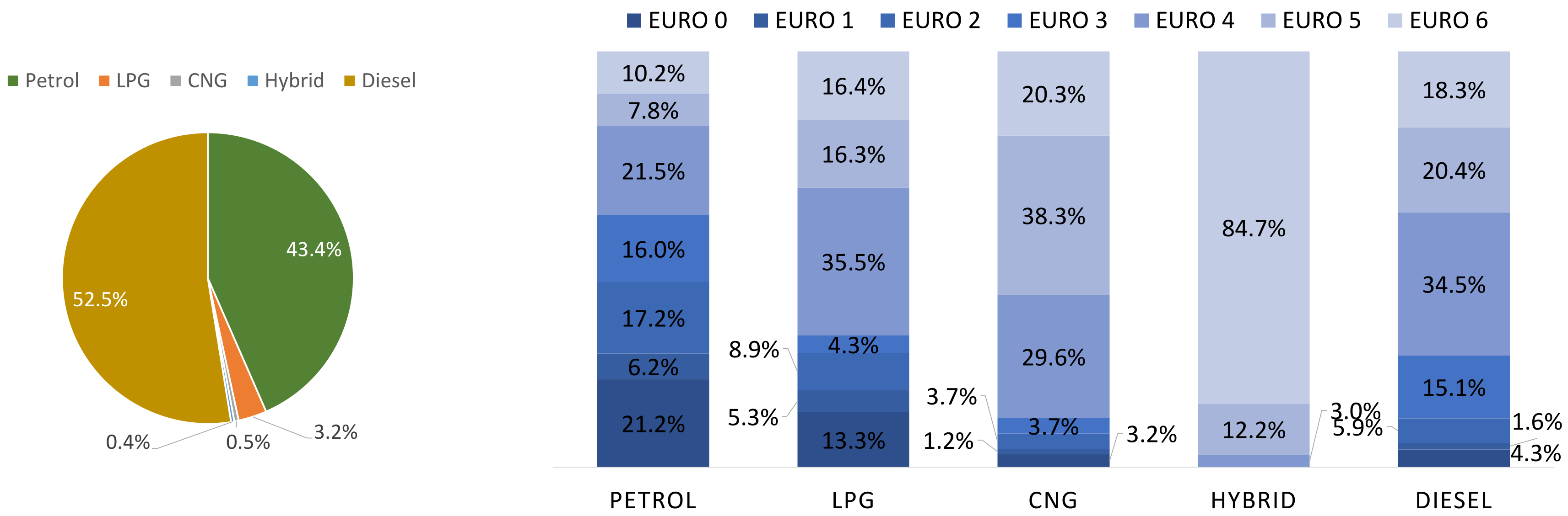
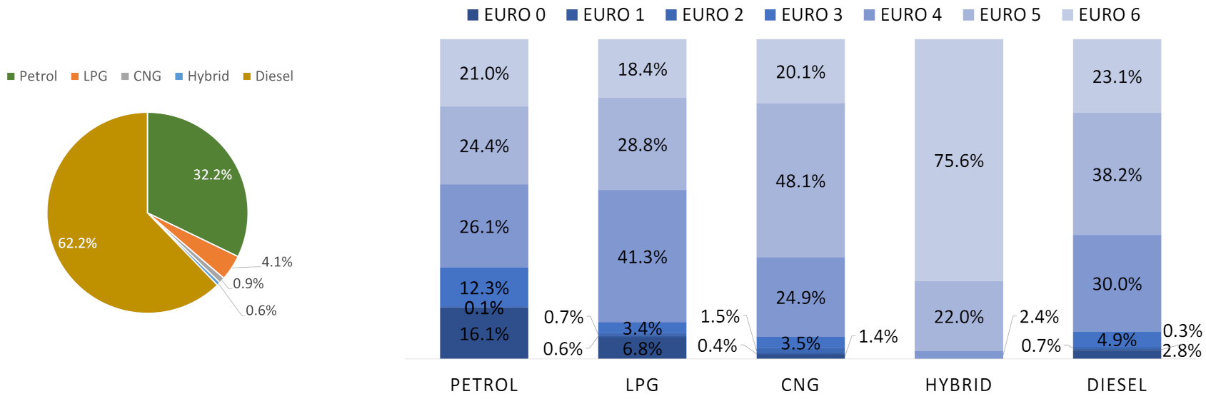
As a result, according to this hypothesis, in 2030, the car fleet is composed of 119.368 vehicles, with a strong reduction of petrol cars (−11.3%) and a significant increase in gasoline ones (+9.7%). The composition of the car fleet, and then the hypothesized scenario, strictly influences the results of the yearly average vehicle and the produced pollutants. However, the proposed methodology can be easily applied to different scenarios, independently from the premises.
The passenger car features in 2019 (reference year) and 2030 are reported in
Figure 2 and
Figure 3, where the distributions by fuel type and emissive technology (emission standards) are depicted.
3.2. Choice of the Statistical Functions
As far as the frequency distribution of the vehicle speed, available studies propose different function forms, especially in an urban context [
29]: a sum of two Gaussian plus an exponential [
30] or a simple Gaussian [
31,
32].
Actually, the different shapes of the distribution depend on the topology of the area [
30]. In particular, in cities that are the origins of commuting travels, the distributions are characterized by more articulated shapes, often with two peaks.
On the contrary, regular shapes are more common in areas that are commuting hubs, where city drivers do not commute daily to a larger city. This scenario suits the example case quite well; therefore, in the proposed application, the Gaussian function was used, also demonstrating to be an acceptable fit in the case of under-saturated flow [
29], typical of the examined context. Therefore, the frequency distribution of the vehicle speed is:
where:
On the other hand, the probability distribution of the distance travelled by passenger cars is of lognormal type [
33,
34]:
where:
is the mean of the y probability distribution, with
is the standard deviation of the y probability distribution.
The mean and standard deviation of all the variables used to build up the probability distribution curves are reported in
Table 1 [
19].
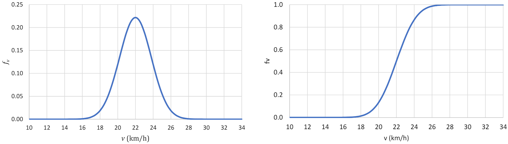
In order to show the trend of the probability curves,
Figure 4 and
Figure 5 depict the graph of both the density and cumulative functions of the random variables’ vehicle speed and daily travelled distance.
3.3. Results
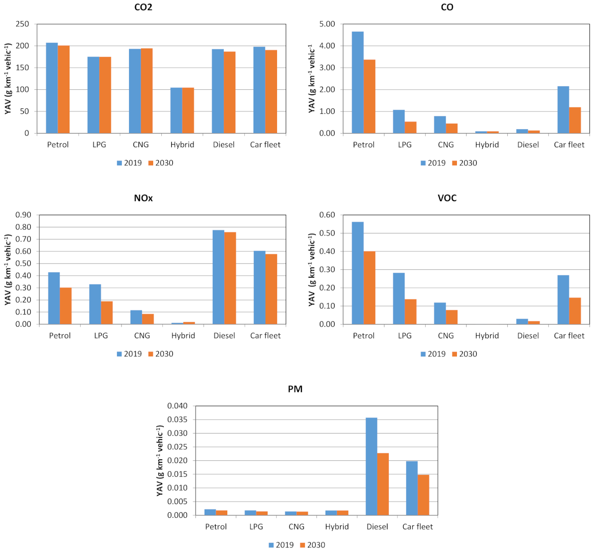
In
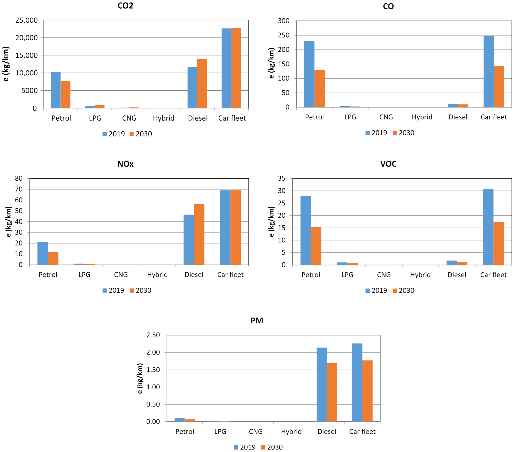
Figure 6, YAVs, calculated with Equation (8) for various pollutants and fuel types, are reported, depicting both the 2019 scenario and its evolution outcome in 2030.
The indicator accounts for the contribution of the specific pollutant emission of the average vehicle, belonging to each considered category.
As a matter of fact, from
Figure 6, it can be inferred that, potentially, all the fuels have a remarkable impact in terms of CO
2 emissions, whereas the petrol average vehicle is responsible for the greatest contribution to both CO and VOC releases. On the contrary, the diesel-fuelled average vehicle is responsible for the highest NO
x and PM productions. This information can be pivotal when actions changing the fleet composition are to be undertaken, so that decision-making processes can be effectively guided.
In this context, it is worth highlighting that, as far as hybrid vehicles are concerned, they have a small share within the car fleet (0.07%), they are all full hybrid type, and hence, the assessed specific emissions are related only to the petrol contribution.
Considering the high number in the single category, the global emissions of the pollutant , in 2019 and 2030, for fuel type and per unit path length, Equation (9), can be estimated.
In this case, the contribution of every vehicle category to the passenger car fleet emissions can be inferred. Specifically, given the share of both petrol and diesel passenger cars in the fleet composition (
Figure 2), major emissions are due to these types of vehicles. Therefore, the impact of the numerousness of each category can be appreciated.
From this perspective, it is worth underlining that, despite the increased number of vehicles occurring within the fleet from 2019 to 2030, the increase in the share of the less emissive classes (
Figure 2 and
Figure 3), which also takes place during the same period of time, produces a reduction of the discharged pollutant emission rates. In other words, this is the outcome generated by the improvement of the whole passenger car fleet emissive quality.
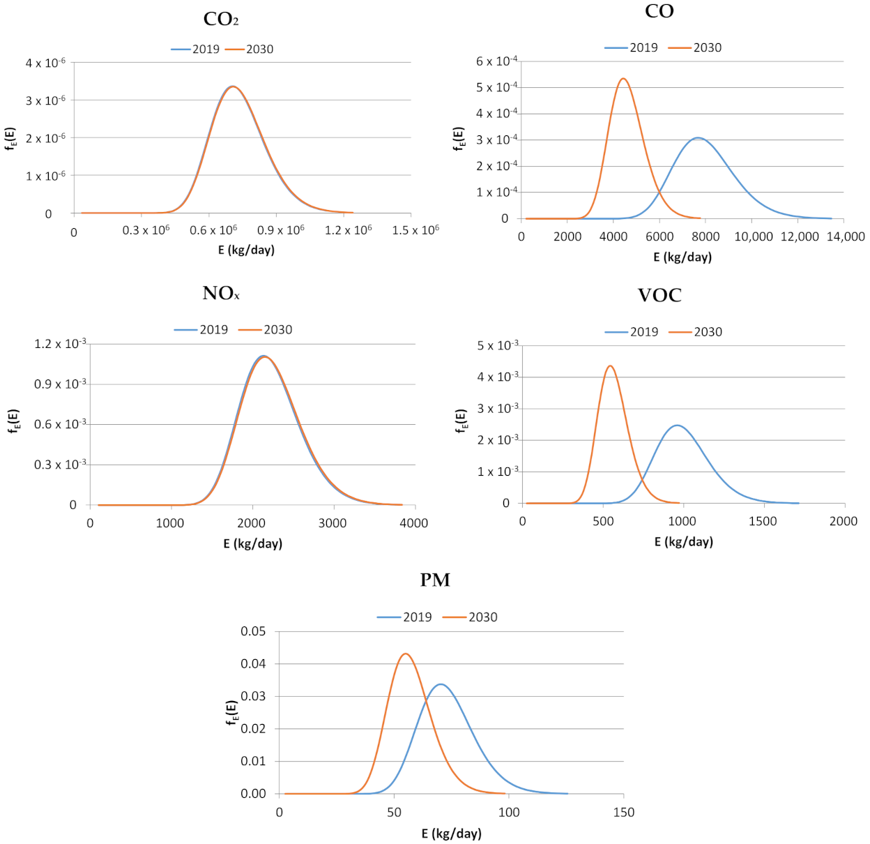
When the mileage probability density distribution Equation (20) is considered, and Equation (14) is applied, the probability density function
depicted in
Figure 8 can be inferred. It is referred to as the whole fleet, under the hypothesis that the probability density function of the variable
,
, is the same for all the vehicle categories composing the fleet.
This is a sufficiently reliable hypothesis for the analysed context, which concerns a small town where, owing to homogeneous demographic factors and reduced transport options, the features of the passenger cars’ daily paths are quite uniform for the various vehicle categories.
Figure 8 shows that, as the passenger car fleet evolves from 2019 to 2030, the probability density distributions of CO, VOC and PM emission rates (
) change appreciably, shifting towards smaller values of
and less disperse shapes. This testifies an improvement of the vehicle emissive quality over time.
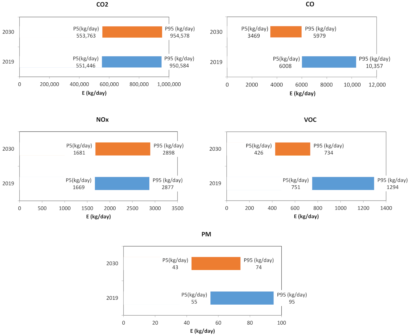
Similar conclusions can be drawn analysing the trend of the percentiles P95 and P5, namely the emission rates, which have probabilities of 5% and 95% to overcome. They are calculated by means of Equation (15) and allow the variability range of each pollutant emission rate to be estimated (
Figure 9). As a matter of fact, it is delimited by the P95 and P5 values, and involves the emission rates values characterized by an occurrence probability higher than 5%, and lower than 95%.
It can be noted that the range of probable values of emission rates shrinks for CO, VOC, and PM, as the car fleet evolves from 2019 to 2030, and the share of the most emissive vehicle categories tends to decrease.
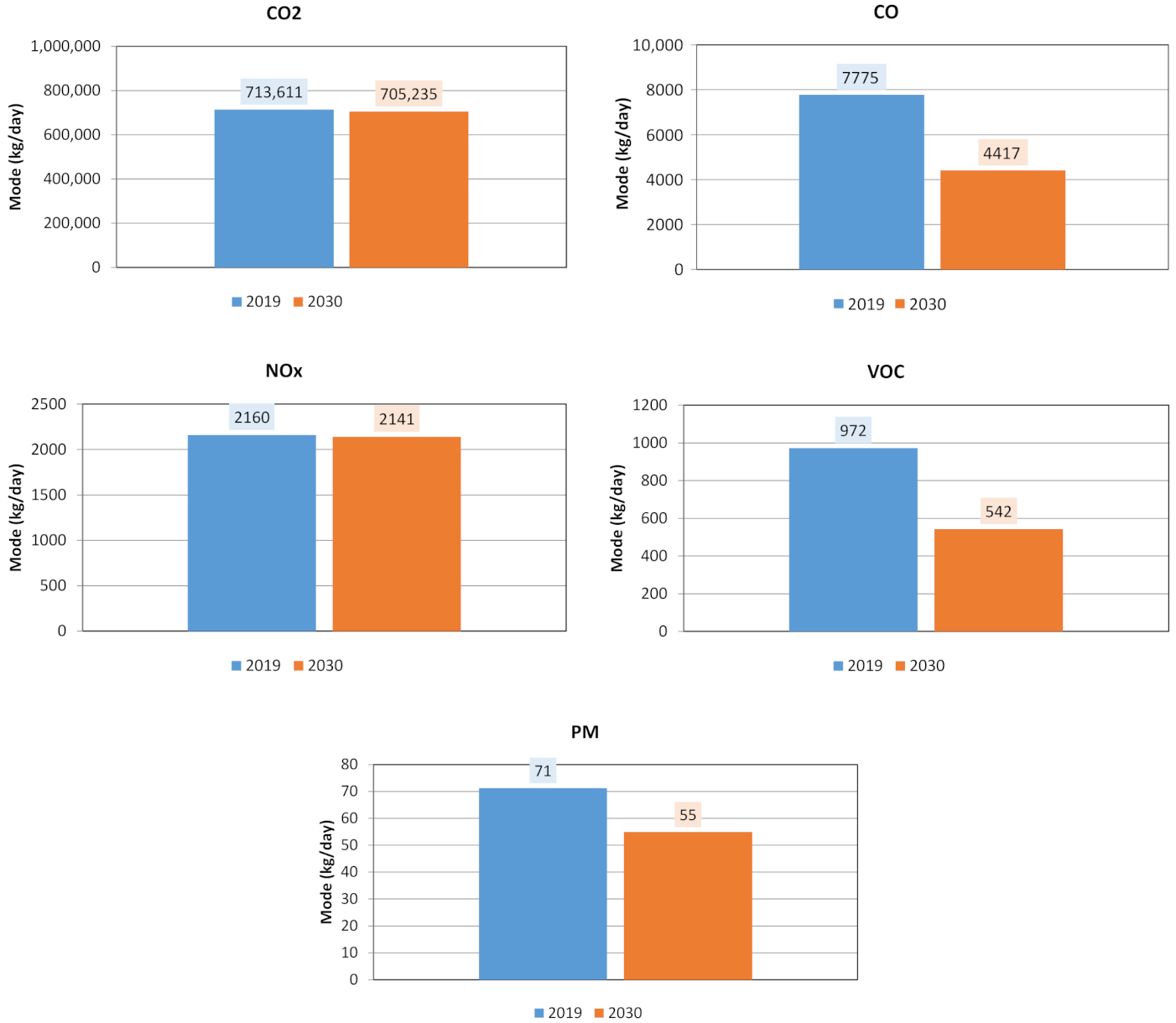
As far as the most probable value of the emission rate is concerned,
Figure 10 reports the variable mode, which is the value with the highest probability of occurrence. It decreases in 2030 for all the considered pollutants.
In conclusion, both the P5–P95 variability range and the emission rate modal value can be exploited to analyse the trend of the car park development from the emission rate perspective.
They can underpin the decision-making process, when the effect of different actions or measures altering the features, composition, and size of the circulating fleet is to be assessed.
4. Conclusions
The analysis of the global amount of pollutant emissions released by road traffic is a crucial aspect of the planning actions aimed at mitigating air pollution and greenhouse gas emissions, especially in urban settlements, which are deemed to be among the human activities, which exert the most deeply spoiling impacts on the environment.
From this point of view, mobility planning may play a pivotal role; however, to reach the objective, it should entail methods and procedures to estimate road traffic emission rates by indicators, measuring the impact that envisaged action may have on the improvement of the air quality.
In this context, a method for the assessment of the pollutant emission rate due to the road traffic was proposed. It involves a statistical approach to consider the influence of traffic parameters that are characterized by a statistical variability: vehicle speed and length of the travelled route in a specific period.
Specifically, the methodology is aimed at the assessment of the probability density function fE(E) of the emission rates E, discharged by the road traffic in a specific spatial context. This last function allows a different approach to be introduced in the analysis of air pollution: knowing the function fE(E), various statistical indicators, (e.g., percentiles, confidence intervals, etc.) can be assessed, so that an in-depth evaluation of different possible scenarios can be related to their occurrence probability.
As a matter of fact, the outcome of the proposed procedure consists of a set of indicators that allows different aspects of the involved phenomena to be estimated. These indicators regard: the pollutant emissions of the average vehicle of the fleet (YAV) referred to the whole range of possible speed values; the emission rate per mileage unit; the most probable emission rate considering the statistical variability of the distance travelled by each vehicle; the extent of the variability range of the possible emission rate values.
All the indicators can be referred to as the whole fleet or to a single homogeneous category, depending on either the type of performed analysis or the vehicle fleet features. In addition, each indicator is related to a single pollutant.
The method was applied to an example case study, so that an account of its suitability was given to assess the effects of the evolution of the passenger car fleet in a medium-sized city located in Southern Italy, according to a possible scenario.
The example demonstrated the suitability of the proposed methodology for analysis involving different perspectives. As a matter of fact, not only were possible improvements of the fleet able to be assessed and compared to the base scenario (by means of the YAV), but the calculated percentiles also allowed the appraisal of the emission rate variability ranges, and of the related occurrence probabilities.
This type of information can play a pivotal role, with a view to supporting and guiding the decision-making process aimed at singling out the best course of action to curb air pollution, because each designed measure can be related to the probability of reducing the emission rates, taking into account the random variability of the involved phenomena.
A hierarchy of the various possible measures and actions can be hence performed on the basis of these probability values.
In this direction, the development of the research activity has been being designed.


