Optimization of Wall Thickness Based on a Comprehensive Evaluation Index of Thermal Mass and Insulation

Abstract

The thermal performance of buildings in the south of China focuses on thermal mass design, while in the north it favors thermal insulation design, which makes it impossible to achieve a balance between the thermal mass and insulation. Here, a comprehensive evaluation index is developed to measure the thermal performance of a building’s external envelope, which aims to find out the optimal range of the wall thickness under the influence of the thermal mass and insulation, and to seek the correct balance between a building’s energy consumption and the thermal performance of walls. In this paper, four dimensions, namely the heat transfer coefficient, thermal inertia index, attenuation degree, and delay time, are discussed, and the weight coefficients of each subfactor are calculated and isotropically treated to create comprehensive evaluation indicators. Then the distribution laws of the composite index values of common building materials in different climatic zones are examined. The result shows that the correlation coefficient (R²) between M and building energy consumption is about 0.7736–0.8215, which is higher than 0.3494–0.384, the heat transfer coefficient, and is more accurate in predicting building energy demands. Furthermore, through the analysis of the thermal improvement rate and the building energy-saving rate, the suitable wall thickness of commonly used building materials in different climate zones is determined, and the application prospects of the research results are described. With the above research findings, the thickness ranges of walls can be determined at the initial period of building design by combining regional environmental factors and material characteristics to provide a reference for building energy-saving design.

1. Introduction

The rapid development of the social economy has significantly accelerated urbanization in China, resulting in considerable energy consumption and carbon emissions [1]. According to the statistics, China’s building energy consumption has risen from 21% to 33% of total energy consumption in the past decade [2,3], leading to negative impacts on the economy and environment. In light of this, the concept of a building’s energy savings has become a primary concern for the built environment, and has a significant potential for energy conservation and emission reductions.

Prompted by the policy of energy conservation and emissions reduction, various regions in China have launched building energy-saving design standards successively. Energy-saving design requirements have also evolved from the 30% in 1986 to the 75% raised in the latest standard (JGJ 26-2018) implemented on 1 August 2019 [4,5]. The thermal performance of a building envelope is the key factor influencing building energy consumption, improvements to which can reduce the amount of energy required to heat and cool interior spaces and may therefore play a significant role in reducing overall energy consumption. Building energy efficiency standards [5,6] require the finite value of the heat transfer coefficient of the building envelope.

Research on the improvement of the thermal performance of the building envelope primarily focuses on the optimization of the thermal insulation performance of building envelopes. Kaynakli [7] optimized the thickness of wall insulation in different heat supply models. Dylewski [8] analyzed the effect of different insulation materials on building energy consumption and specifically optimized the thickness of composite walls. Additionally, Daouas [9] studied the effect of environmental factors on the heat transfer coefficient of the building envelope and modified it. Furthermore, Song et al. [10] used the economic net present value (NPV) method to evaluate different envelope modification methods. Zhang et al. [11] analyzed the effect of different material insulation and construction forms on building energy consumption using an energy simulation method and constructed an economic optimization method in Chengdu. Moreover, Dodoo et al. [12] analyzed the relationship between the building envelope economy and building energy consumption from the perspective of the whole building life cycle, and optimized the selection of materials for the economy. Subsequently, Arnas Majumder [13] studied the optimization of recyclable material insulation panels and proved the feasibility of the technological routes.

Unlike thermal insulation, which has been studied extensively, the thermal mass and its effects on a building’s energy and thermal performance are yet to be researched comprehensively [14]. Zhu et al. [15] studied the thermal mass of the envelope and found that the effective use of the thermal mass could significantly reduce a building’s energy consumption. Ghoreishi [16] found that a building envelope with a high thermal mass could induce a significant thermal lag, delaying the effect of peak temperatures and reducing the amplitude of the heat gain, which results in reductions in seasonal heating and cooling loads. Additionally, Al-Sanea et al. [17] studied thermal mass insulated wall buildings and showed that the buildings were relatively energy efficient in the spring and autumn seasons, but not in summer and winter. Dodoo et al. [18], Wang et al. [19], Reilly and Kinnane [20], and Deng et al. [21] studied the thermal mass of buildings in specific climatic zones, the their results showed that in hot summer and cold winter regions or hot regions, the increase of the thermal mass could effectively reduce a building’s cooling energy consumption, and the advantages were better highlighted in areas with a large temperature difference between day and night. Hoes, Trcka, Hensen, and Bonnema [22,23] studied the effects of a high thermal mass on the reduction of overheating in a mid-European climate, where heating may not be the governing design factor. Furthermore, some other scholars studied the effect of the thermal mass and insulation through construction layers of different thicknesses, but these studies were never able to respond positively to the effect of the thermal mass on the energy demand in cold climates [16,24,25,26].

Moreover, although coupling the thermal mass with code-required thermal insulation commonly and inherently takes place in everyday construction projects, only a few studies have comprehensively discussed the impact of such a combination on a building’s energy use in a generalizable manner, resulting in increased errors in predicting energy consumption at the beginning of the building’s design [27,28].

To resolve these limitations, this article presents a study of a comprehensive index evaluating the effect of a material’s thermal mass—in conjunction with thermal insulation—on the overall energy performance of residential buildings across a range of climate zones in China. It considers the characteristics of buildings’ exterior walls, as the interface between indoor and outdoor energy exchange, to assess the impact of these parameters on annual energy demands. By using the comprehensive evaluation index, coupled with the thermal mass with insulation, the thermal performance of conventional building materials in five main Chinese climate zones could be quantified.

In summary, this study is theoretical research focusing on varying building construction parameters, such as wall thickness, to investigate the effect of coupling thermal mass with insulation on a building’s energy performance, but not necessarily the building’s practical design. The purpose of this paper is to find a method combining the thermal mass and insulation to evaluate the performance of building materials and to discover the correlation between it and building energy demands. It also aims to give the appropriate wall thickness interval for different materials in five main climate zones, with the factors of the comprehensive index improvement and energy-saving rate of a building’s energy consumption, to provide a reference for the energy-saving design of a building at the early stage of its design.

2. Research Methodology

To establish a comprehensive evaluation index of the thermal mass and insulation, Four relevant metrics, namely the heat transfer coefficient, thermal inertia index, temperature wave attenuation, and phase detention time, were taken. For this paper, five common building materials, namely reinforced concrete, aerated concrete, rammed earth, clay brick, and hollow clay brick were selected, and, based on the above comprehensive evaluation index, the design interval of a building structure’s thickness suitable for the typical cities of different thermal zones are given in combination with the room ambient design temperature. In addition, the energy demands were simulated with WUFI plus to prove the comprehensive evaluation index.

2.1. Materials and Properties

Taking the “Code for thermal design of the civil building’’ as a reference [29], the density, thermal conductivity, specific heat capacity, and thermal storage coefficient of the above five building materials are listed, as shown in

Table 1. Physical parameters of five materials.

No.	Name	Dry Density (kg/m3)	Specific Heat Capacity KJ/(kg·K)	Thermal Conductivity (W/m·K)	Thermal Storage Conductivity (W/(m2·K)
1	Reinforced concrete	2500	0.92	1.74	17.20
2	Aerated concrete	700	1.05	0.18	3.10
3	Rammed earth	2034	1.28	0.74	11.85
4	Clay bricks	1800	1.05	0.81	10.63
5	Hollow clay brick	1400	1.05	0.58	7.92

.

2.2. Typical Cities in the Thermal Zones

Thermal zones in China can be roughly divided into a hot summer and warm winter zone, a mild zone, a hot summer and cold winter zone, and cold and harsh regions, and five cities—namely Guangzhou, Kunming, Shanghai, Beijing, and Harbin—were selected in turn as typical representative cities in each thermal zone. The climatic parameters of the typical cities are shown in

Table 2. Typical city and meteorological parameters.

No.	Zone and City	Relative Humidity φs (%)	Wind Speed V(m/s)	Average Temperature T (°C)	Daily Solar Radiation (MJ/m2)
1	Hot summer and warm winter: Guangzhou	78.4	1.88	21.5	12.8
2	Mild region: Kunming	66.0	1.98	13.9	14.5
3	Hot summer and cold winter: Shanghai	74.5	3.15	19.7	13.2
4	Cold regions: Beijing	57.6	2.05	13.5	10.4
5	Harsh cold areas: Harbin	59.7	3.05	3.3	9.6

[30].

2.3. Base Case Model

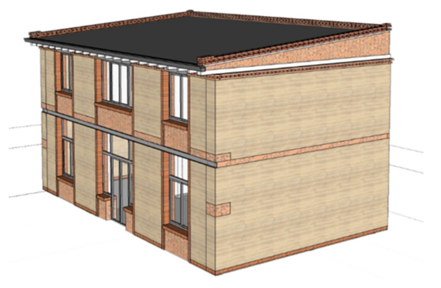
This paper uses a two-story house as a prototype for the energy simulation to study the effect of different thicknesses of walls on the energy demand of a building, which is similar in scale to the majority of residential houses in China. Its length, width, and height of the building are 12.9 m, 7.7 m, and 6.3 m, respectively; the height of the ground floor is 3.6 m and that of the first floor is 3.3 m. The appearance of the building is shown in Figure 1, with each floor of the building consisting of three main thermal zones: a separate bedrooms on each side and an open living room in the middle.

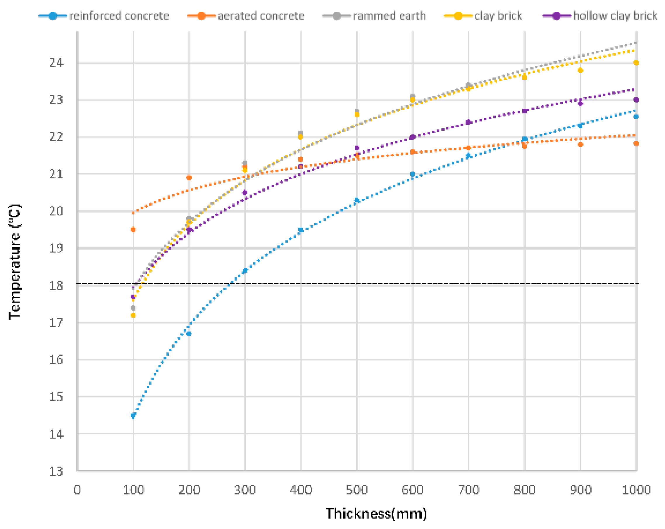
To assess the impact of the thermal mass and insulation of different materials within various wall constructions on the energy demand, ten different external wall thicknesses were chosen, namely 100, 200, 300, 400, 500, 600, 700, 800, 900, and 1000 mm. The specifications of the base case model are seen in

Table 3. The specifications of the base case model.

Residential Houses
Window-to-wall ratio (%)	South:28.0	North:10.8	East: 0.0	West:0.0
People density (people/m2)	0.025
Wall U-value (W/m2 K)	Value varies with thickness
Window U-value (W/m2 K)	2.0
Floor U-value (W/m2 K)	0.2
Roof U-value (W/m2 K)	0.25
Heating setpoint (°C)	18
Cooling setpoint (°C)	26
HVAC schedule	Mon.–Fri.: 17:00–9:00; weekend: 0: 00–24:00
Ventilation (1/h)	0.8

.

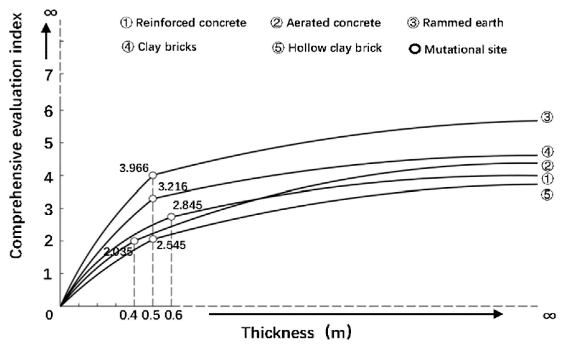
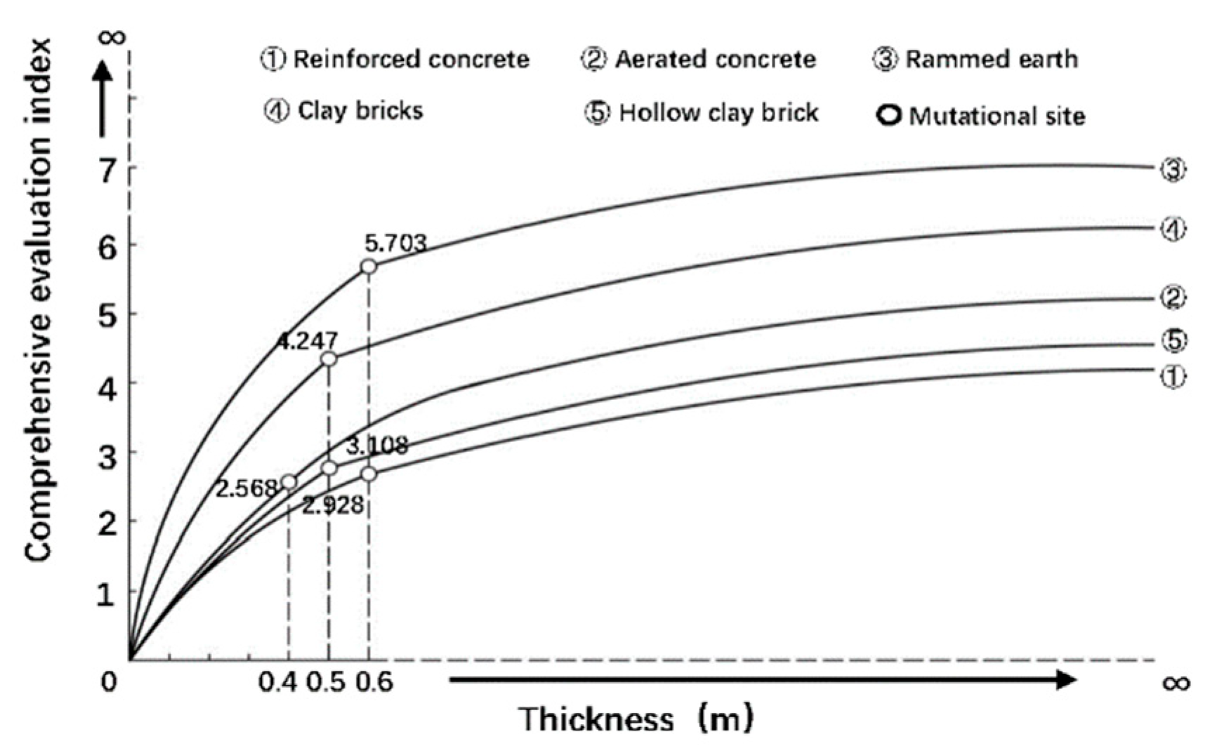
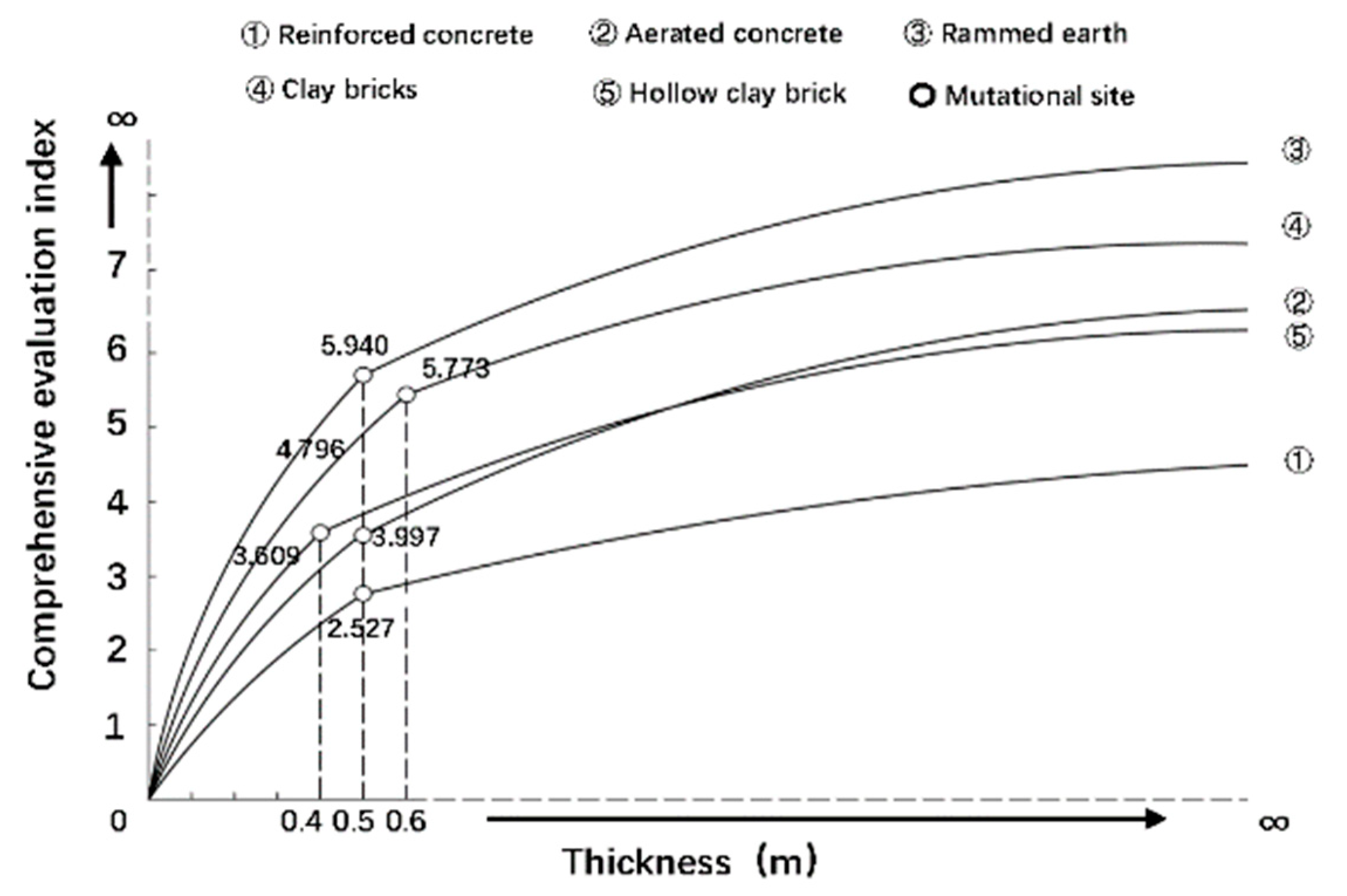
2.4. Comprehensive Evaluation Index

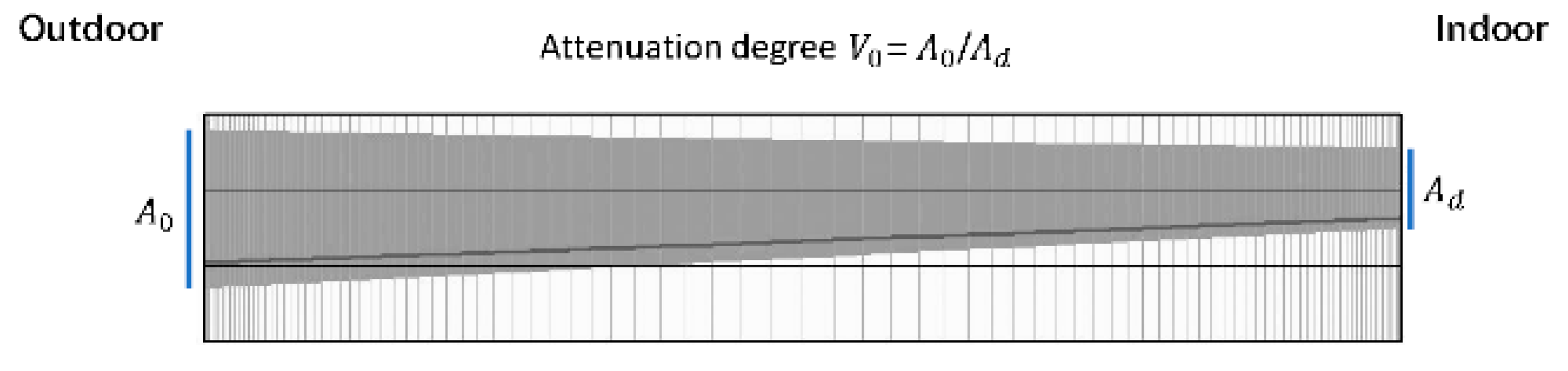
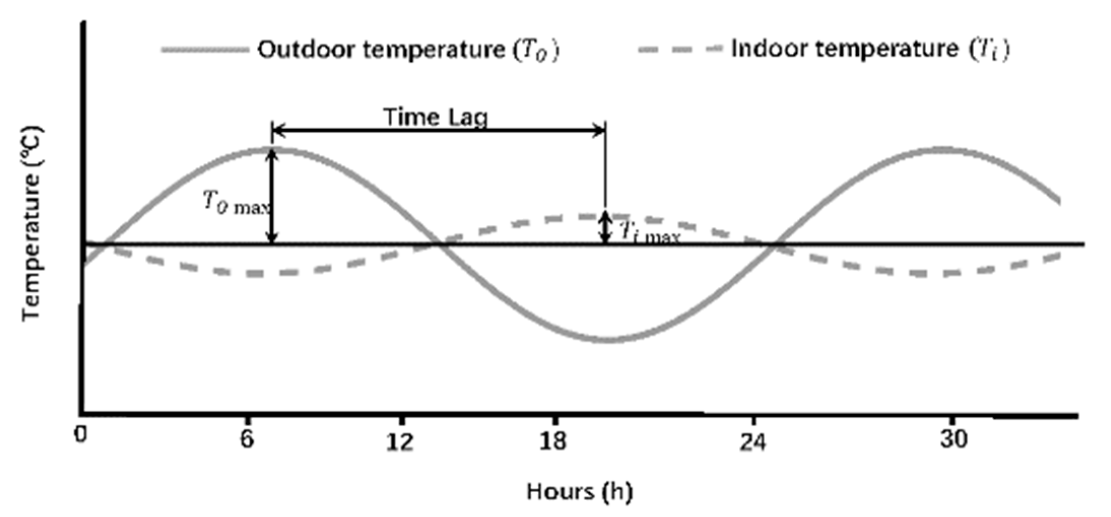
It is well known that the thermal performance of wall materials is mainly measured by their thermal mass and insulation. The wall insulation performance depends on the heat transfer coefficient of the wall, and the heat storage coefficient of the material is the key factor affecting the thermal mass of the wall. With the same thermal storage coefficient, the greater the thermal inertia index and temperature wave attenuation, the longer the phase detention time, and the better the thermal performance of the wall are. Through the derivation of the formula, it can be found that the above factors are all related to the thickness of the wall. Therefore, with the thickness as the only variable, a comprehensive evaluation index was established with four parameters, namely the heat transfer coefficient, thermal inertia index, temperature wave attenuation, and phase detention time, seen in Equation (1):

M = a·β_1/U + b·β_D + c·β_V0 + e·β_ξ

(1)

where, a, b, c, and e represent the sensitivity coefficients of the above parameters with respect to the change in wall thickness, respectively. β represents the linear relationship after the dimensionless treatment of each subfactor.

3. Calculation and Simulation

In this subsection, we describe in turn how the heat transfer coefficient, attenuation degree, thermal inertia index, and delay time of different material walls were calculated, the sensitivity coefficients of each parameter were extracted and expressed in the form of a comprehensive evaluation index, and the relationship between the thermal performance of walls and wall thickness was then analyzed; the thickness interval of walls for each material under the condition of achieving the specification requirements is then discussed in conjunction with the requirements of the indoor thermal environment in different thermal zones.

3.1. Discussion of Subfactors

3.1.1. Divergence Analysis of U-Value

The heat exchange condition between the surface of the building and the surrounding environment is relatively complex and can be roughly divided into the following three forms:

(a)

The radiation heat exchange: There are three main modalities of the radiation heat exchange of buildings, one of which is heat absorption by buildings under the action of solar short-wave radiation; another is heat absorption under the action of atmospheric long-wave radiation; and the third is the radiation heat exchange between the wall surface and the environment. The radiation heat transfer between the building and the surrounding environment is a complex process, but its radiation heat transfer coefficient can be calculated in a simplified way as in Equation (2):

α_r = Ċθ

(2)

where α_r is the radiation heat transfer coefficient, W/(m²·K); Ċ is the radiation coefficient of the two objects involved in radiation; the value of general building materials is 4.0 W/(m²·K⁴); and θ is the temperature factor and takes the value of 1.2 h·k³.

(b)

The convection heat exchange: the heat exchange under the action of atmospheric convection and the coefficient of convection heat transfer changes with the change of airflow rate can be calculated according to Equation (3):

α_q = 6.31v^0.656 + 3.25e^−1.91v

(3)

where α_q is the convective heat transfer coefficient, W/(m²·K); v is the average wind speed of the outdoor environment, m/s; and e is a constant, taking the value of 2.718.

(c)

The latent heat of evaporation: the heat exchange caused by the evaporation of water vapor. The evaporative heat transfer coefficient can be calculated according to Equation (4):

α_m = 1.954φ_s·α_q

(4)

where α_m is the evaporative heat transfer coefficient, W/(m²·K), and φ_s is the relative humidity of the wall surface, whose value is taken to approximate the ambient relative humidity.

In summary, the formula for calculating the heat transfer coefficient on the outside surface of the wall is shown in Equation (5):

α = α_r + α_q + α_m

(5)

By Equation (5), the heat transfer coefficient of the external surface of the building in each typical city was calculated, as shown in

Table 4. Typical city and outdoor surface heat transfer coefficients.

No.	City	αq W/(m2·K)	αr W/(m2·K)	αm W/(m2·K)	α W/(m2·K)	External Surface Heat Transfer Resistance (Re) (m2·K)/W
1	Guangzhou	9.64	4.8	14.76	15.22	0.066
2	Kunming	9.95	4.8	12.83	15.41	0.065
3	Shanghai	13.40	4.8	19.51	19.95	0.053
4	Beijing	10.17	4.8	11.45	15.55	0.064
5	Harbin	13.12	4.8	15.32	18.52	0.054

The internal surface heat transfer resistance is taken to be R_i = 0.11 (m²·K)/W [29].

.

3.1.2. Thermal Lag in Different Zones

The thermal lag depends on the thermal mass and resistance of the material. Therefore, the thermal inertness indexes of the above five materials were approximately equal in the different sub-regions, and could be calculated based on Equation (6):

D = R·S

(6)

where D-value is a dimensionless datum; R is the thermal resistance of the material layer, (m²·K)/W, and S is the heat storage coefficient of the material, which is related to the specific heat, density, and thermal conductivity of the material, W/(m²·K).

3.1.3. Definition of Temperature Wave Attenuation

As shown in Figure 2, the ratio of the harmonic amplitudes of the external and internal surface temperatures of the wall was used to measure the attenuation effect of the walls of different thicknesses on the temperature wave. The value was defined as the average annual attenuation of the temperature wave V₀, seen Equation (7):

V₀ = A₀/A_d

(7)

where A₀ is the annual temperature amplitude of the external surface of the wall and A_d represents the annual temperature amplitude of the internal surface of the wall.

3.1.4. Calculation of Time Lag

The time delay is due to the thermal mass, and the thicker and more resistive the material, the longer the time lag was. The heat transfer coefficient of the inner and outer surfaces of the wall also led to differences in the time lag of the materials in different thermal zones.

As seen in Figure 3, the delay time refers to the interval between the appearance of the peak outdoor temperature wave and the appearance of the peak temperature of the inner surface of the external wall. The delay time of walls made of different materials was calculated according to Equation (8):

$$\xi =\frac{Z}{360}\left(40.5\sum D+arctan\frac{Y_{ef}}{Y_{ef}+\sqrt{2}{\alpha }_e}-arctan\frac{{\alpha }_i}{{\alpha }_i+\sqrt{2}{Y}_{if}}\right)$$

(8)

where Z is the time cycle, taking the value of 24 h; D is the thermal inertness index of the material; Y_ef is the heat storage coefficient of the external surface of the wall, W/(m²·K); α_e is the heat transfer coefficient of the external surface of the wall, W/(m²·K); Y_if is the heat storage coefficient of the internal surface of the wall, W/(m²·K); and α_i is the heat transfer coefficient of the internal surface of the wall, W/(m²·K).

3.2. Calculation in Different Zones

Here, we describe how the parameters were calculated for each of the five cities in turn and analyzed linearly.

3.2.1. Hot Summer and Warm Winter: Guangzhou

(a)

Thickness and U-Value

We combined the data in Table 4 and the WUFI Pro software to calculate the heat transfer coefficients of the above five materials, using the quotient method and the mean method to invert and dimensionlessly process the data; the results are shown in

Table 5. The relation between thickness and U-value in Guangzhou.

No.	100	200	300	400	500	600	700	800	900	1000
U1	3.91	3.38	2.98	2.66	2.35	2.15	1.98	1.83	1.68	1.57
1/U1	0.26	0.30	0.34	0.38	0.43	0.47	0.51	0.55	0.60	0.64
U2	1.36	0.80	0.56	0.44	0.36	0.30	0.26	0.23	0.20	0.18
1/U2	0.74	1.26	1.78	2.30	2.81	3.36	3.88	4.38	5.03	5.59
U3	3.17	2.24	1.71	1.40	1.18	1.01	0.89	0.80	0.72	0.66
1/U3	0.32	0.45	0.59	0.72	0.85	0.99	1.13	1.26	1.40	1.53
U4	2.98	2.19	1.71	1.42	1.21	1.05	0.93	0.83	0.75	0.70
1/U4	0.34	0.46	0.59	0.71	0.83	0.96	1.08	1.21	1.33	1.44
U5	2.73	1.90	1.46	1.20	1.00	0.87	0.77	0.68	0.61	0.56
1/U5	0.37	0.53	0.69	0.84	1.00	1.15	1.31	1.48	1.64	1.78

.

A linear fit to the heat transfer coefficient values gave the following sensitivity coefficients for different materials as the wall thickness varied: a₁ = 0.408, a₂ = 0.885, a₃ = 0.701, a₄ = 0.65, and a₅ = 0.701.

(b)

Thickness and D-Value

The thermal inertia index is dimensionless and numerically equal to the product of the material’s heat storage coefficient and thermal resistance. The thermal inertia indexes of reinforced concrete, aerated concrete, rammed earth, clay brick, and hollow clay brick were calculated separately and are shown in

Table 6. The relation between thickness and D-Value.

No.	100	200	300	400	500	600	700	800	900	1000
D1	0.99	1.98	2.97	3.95	4.94	5.93	6.92	7.91	8.90	9.89
D2	1.72	3.44	5.17	6.89	8.61	10.33	12.56	13.78	15.50	17.22
D3	1.66	3.20	4.86	6.40	8.06	9.60	11.26	12.80	14.46	16.00
D4	1.31	2.63	3.94	5.25	6.56	7.87	9.19	10.50	11.81	13.12
D5	1.37	2.73	4.10	5.46	6.83	8.19	9.56	10.92	12.29	13.66

. It can be seen that the thermal inertia index of the wall was directly proportional to the wall thickness, and the sensitivity coefficients of each material were as follows: b₁ = 0.001, b₂ = 0.017, b₃ = 0.016, b₄ = 0.013, and b₅ = 0.014.

(c)

Thickness and Attenuation degree

Here WUFI Pro was used to simulate the heat and moisture transfer process of the walls under different thicknesses; the annual variation range of the internal and external surface temperature of the wall was obtained by simulation, then attenuation degrees were calculated according to Equation (7). The results are shown in

Table 7. The relation between thickness and attenuation degree.

No.	100	200	300	400	500	600	700	800	900	1000
V1	1.33	1.78	2.21	2.63	3.07	3.67	4.00	4.4	4.49	4.58
V2	2.78	3.25	3.33	3.47	3.56	3.71	3.77	3.82	3.88	3.94
V3	2.00	2.56	3.29	4.00	4.14	4.44	4.62	4.71	4.90	5.00
V4	1.83	2.77	3.38	3.83	4.14	4.36	4.62	4.80	4.90	4.95
V5	2.05	2.88	3.20	3.43	3.53	3.58	3.69	3.69	3.72	3.75

.

The sensitivity coefficient for the attenuation of each material was determined by a linear fit: c₁ = 0.581, c₂ = 0.144, c₃ = 0.413, c₄ = 0.426, and c₅ = 0.241.

(d)

Thickness and Delay Time

According to Equation (8), the delay times of different materials for temperature waves were calculated in turn and the results are shown in

Table 8. The relation between thickness and delay time.

No.	100	200	300	400	500	600	700	800	900	1000
ξ1	2.69	5.52	8.27	10.98	13.68	16.37	19.05	21.73	24.41	27.09
ξ2	3.29	7.82	12.42	17.04	21.67	26.31	30.95	35.6	40.24	44.89
ξ3	4.14	8.55	12.91	17.26	21.6	25.93	30.26	34.59	38.92	43.24
ξ4	3.24	6.85	10.43	13.99	17.55	21.1	24.65	28.19	31.74	35.29
ξ5	3.12	6.81	10.49	14.18	17.86	21.55	25.24	28.92	32.61	36.30

.

According to the data in Table 8, the corresponding coefficients were obtained: e₁ = 0.027, e₂ = 0.046, e₃ = 0.043, e₄ = 0.036, and e₅ = 0.037.

(e)

Thickness and M_GZ

The data were handled dimensionlessly and the values of the comprehensive indexes of different building materials in Guangzhou were calculated; the main trends are shown in Figure 4. The results show that with the increase of wall thickness, the thermal behavior benefits presented by different materials varied, and the performance gains were ordered so: if the thickness of the wall was less than 750 mm, then ③ > ④ > ① > ② > ⑤; otherwise, ③ > ④ > ② > ① > ⑤.

At the mutational site, specific values of the wall thickness allowed for maximum thermal performance benefits.

3.2.2. Mild Region: Kunming

(a)

Thickness and U-Value

The heat transfer coefficients of walls of different materials in the Kunming area were calculated according to the method above, and the results are shown in

Table 9. The relation between thickness and U-value in Kunming.

No.	100	200	300	400	500	600	700	800	900	1000
U1	3.92	3.39	2.99	2.67	2.35	2.15	1.98	1.84	1.68	1.58
1/U1	0.25	0.29	0.33	0.37	0.42	0.46	0.50	0.54	0.59	0.63
U2	1.36	0.80	0.56	0.44	0.36	0.30	0.26	0.23	0.20	0.18
1/U2	0.73	1.25	1.77	2.29	2.80	3.35	3.87	4.37	5.02	5.58
U3	3.18	2.25	1.71	1.40	1.18	1.02	0.89	0.80	0.72	0.66
1/U3	0.31	0.44	0.58	0.71	0.84	0.98	1.12	1.25	1.39	1.52
U4	2.99	2.20	1.71	1.42	1.21	1.05	0.93	0.83	0.75	0.70
1/U4	0.33	0.45	0.58	0.70	0.82	0.95	1.07	1.20	1.32	1.43
U5	2.74	1.91	1.46	1.20	1.01	0.87	0.77	0.68	0.61	0.56
1/U5	0.36	0.52	0.68	0.83	0.99	1.14	1.30	1.47	1.63	1.77

.

The sensitivity coefficients of each material were fitted as follows: a₁ = 0.408, a₂ = 0.886, a₃ = 0.701, a₄ = 0.65, and a₅ = 0.702.

(b)

Thickness and D-Value

The thermal inertia index did not change with regional differences, so the thermal inertia index in Kunming was consistent with the above, and the sensitivity coefficients of each material were as follows: b₁ = 0.001, b₂ = 0.017, b₃ = 0.016, b₄ = 0.013, and b₅ = 0.014.

(c)

Thickness and Attenuation degree

As seen in

Table 10. The relation between thickness and attenuation degree.

No.	100	200	300	400	500	600	700	800	900	1000
V1	1.33	1.64	2.24	2.71	3.17	3.45	3.8	3.96	4.22	4.75
V2	2.56	2.94	3.07	3.29	3.38	3.43	3.48	3.54	3.57	3.59
V3	2.00	2.92	3.62	4.40	4.89	5.24	5.37	5.50	5.57	5.64
V4	2.00	2.67	3.39	4.20	4.57	4.67	4.77	4.88	4.94	5.00
V5	2.05	2.63	2.84	2.99	3.67	3.79	3.86	3.93	4.00	4.07

, the attenuation degrees were calculated, and the sensitivity coefficient for the attenuation of each material were determined by a linear fit: c₁ = 0.571, c₂ = 0.146, c₃ = 0.463, c₄ = 0.415, and c₅ = 0.31.

(d)

Thickness and Delay time

The delay times of the different materials were calculated in turn and the results are shown in

Table 11. The relation between thickness and delay time.

No.	100	200	300	400	500	600	700	800	900	1000
ξ1	2.68	5.51	8.26	10.97	13.67	16.36	19.04	21.72	24.40	27.08
ξ2	3.28	7.81	12.41	17.03	21.66	26.3	30.94	35.59	40.23	44.88
ξ3	4.14	8.55	12.91	17.25	21.59	25.92	30.25	34.58	38.91	43.24
ξ4	3.23	6.84	10.42	13.98	17.54	21.09	24.64	28.19	31.73	35.28
ξ5	3.11	6.80	10.48	14.17	17.86	21.54	25.23	28.92	32.60	36.29

. According to the data, the corresponding coefficients obtained are: e₁ = 0.027, e₂ = 0.046, e₃ = 0.043, e₄ = 0.036, and e₅ = 0.037.

(e)

Thickness and M_KM

As shown in Figure 5, the performance gains were ordered as follows: if the thickness of the wall was less than 650 mm, then ③ > ④ > ① > ② > ⑤; otherwise, ③ > ④ > ② > ① > ⑤.

3.2.3. Hot Summer and Cold Winter: Shanghai

(a)

Thickness and U-Value

The heat transfer coefficients of walls of different materials in the Shanghai area were calculated and the results are shown in

Table 12. The relation between thickness and U-value in shanghai.

No.	100	200	300	400	500	600	700	800	900	1000
U1	4.12	3.54	3.10	2.76	2.42	2.21	2.03	1.88	1.72	1.61
1/U1	0.24	0.28	0.32	0.36	0.41	0.45	0.49	0.53	0.58	0.62
U2	1.38	0.80	0.57	0.44	0.36	0.30	0.26	0.23	0.20	0.18
1/U2	0.72	1.24	1.76	2.28	2.79	3.34	3.86	4.36	5.01	5.57
U3	3.30	2.31	1.75	1.42	1.20	1.03	0.90	0.80	0.72	0.66
1/U3	0.30	0.43	0.57	0.70	0.83	0.97	1.11	1.24	1.38	1.51
U4	3.10	2.26	1.75	1.44	1.23	1.06	0.94	0.84	0.76	0.70
1/U4	0.32	0.44	0.57	0.69	0.81	0.94	1.06	1.19	1.31	1.42
U5	2.83	1.95	1.49	1.22	1.02	0.88	0.77	0.68	0.62	0.57
1/U5	0.35	0.51	0.67	0.82	0.98	1.13	1.29	1.46	1.62	1.76

.

The sensitivity coefficients of each material were fitted as follows: a₁ = 0.422, a₂ = 0.892, a₃ = 0.715, a₄ = 0.663, and a₅ = 0.713.

(b)

Thickness and D-Value

The sensitivity coefficients of each material in Shanghai were as follows: b₁ = 0.001, b₂ = 0.017, b₃ = 0.016, b₄ = 0.013, and b₅ = 0.014.

(c)

Thickness and Attenuation degree

As seen in

Table 13. The relation between thickness and attenuation degree.

No.	100	200	300	400	500	600	700	800	900	1000
V1	1.37	1.80	2.24	2.67	3.22	3.63	4.14	4.54	4.92	5.09
V2	3.00	3.78	4.25	4.40	4.86	4.85	5.00	5.07	5.11	5.15
V3	2.00	3.00	3.88	4.57	5.33	6.40	6.73	6.80	6.88	6.95
V4	1.80	2.86	3.66	4.43	5.17	5.52	5.82	6.15	6.40	6.46
V5	2.11	2.73	3.44	3.90	4.10	4.27	4.57	4.71	4.78	4.85

, the attenuation degrees were calculated, and the sensitivity coefficient for the attenuation of each material was determined by a linear fit: c₁ = 0.606, c₂ = 0.231, c₃ = 0.574, c₄ = 0. 565, and c₅ = 0.37.

(d)

Thickness and Delay time

According to

Table 14. The relation between thickness and delay time.

No.	100	200	300	400	500	600	700	800	900	1000
ξ1	2.55	5.38	8.12	10.83	13.53	16.22	18.90	21.58	24.26	26.94
ξ2	3.14	7.67	12.27	16.89	21.52	26.16	30.80	35.45	40.09	44.74
ξ3	4.00	8.41	12.77	17.11	21.45	25.78	30.11	34.44	38.77	43.10
ξ4	3.09	6.71	10.28	13.84	17.40	20.95	24.50	28.05	31.59	35.14
ξ5	2.97	6.66	10.34	14.03	17.72	21.40	25.09	28.78	32.46	36.15

, the corresponding coefficients obtained were: e₁ = 0.027, e₂ = 0.046, e₃ = 0.043, e₄ = 0.036, and e₅ = 0.037.

(e)

Thickness and M_SH

As shown in Figure 6, the performance gains in Shanghai were ordered so: ③ > ④ > ② > ⑤ > ①.

3.2.4. Cold Regions: Beijing

(a)

Thickness and U-Value

The heat transfer coefficients of walls of different materials in the Beijing area were calculated and the results are shown in

Table 15. The relation between thickness and U-value in Beijing.

No.	100	200	300	400	500	600	700	800	900	1000
U1	3.93	3.40	2.99	2.67	2.36	2.15	1.98	1.84	1.68	1.58
1/U1	0.25	0.29	0.33	0.37	0.42	0.46	0.50	0.54	0.59	0.63
U2	1.36	0.80	0.56	0.44	0.36	0.30	0.26	0.23	0.20	0.18
1/U2	0.73	1.25	1.77	2.29	2.80	3.35	3.87	4.37	5.02	5.58
U3	3.18	2.25	1.71	1.40	1.18	1.02	0.89	0.80	0.72	0.66
1/U3	0.31	0.44	0.58	0.71	0.84	0.98	1.12	1.25	1.39	1.52
U4	2.99	2.20	1.71	1.42	1.21	1.05	0.93	0.83	0.76	0.70
1/U4	0.33	0.45	0.58	0.70	0.82	0.95	1.07	1.20	1.32	1.43
U5	2.74	1.91	1.46	1.20	1.01	0.87	0.77	0.68	0.61	0.56
1/U5	0.36	0.52	0.68	0.83	0.99	1.14	1.30	1.47	1.63	1.77

.

The sensitivity coefficients of each material were fitted as follows: a₁ = 0.409, a₂ = 0.886, a₃ = 0.702, a₄ = 0.651, and a₅ = 0.702.

(b)

Thickness and D-Value

The sensitivity coefficients of each material in Beijing were as follows: b₁ = 0.001, b₂ = 0.017, b₃ = 0.016, b₄ = 0.013, and b₅ = 0.014.

(c)

Thickness and Attenuation degree

As seen in

Table 16. The relation between thickness and attenuation degree.

No.	100	200	300	400	500	600	700	800	900	1000
V1	1.45	1.89	2.36	2.96	3.40	3.80	4.12	4.38	4.60	4.79
V2	3.12	4.35	5.26	5.56	5.88	6.16	6.35	6.50	6.67	6.77
V3	2.12	3.27	4.22	4.8	5.57	5.97	7.2	8.04	8.71	9.09
V4	1.97	2.95	4.11	4.69	5.43	6.13	6.91	7.60	7.92	8.44
V5	1.94	2.68	3.22	3.90	4.39	5.00	5.36	5.51	5.68	6.00

, the attenuation degrees were calculated, and the sensitivity coefficient of each material could be drawn by a linear fit: c₁ = 0.533, c₂ = 0.322, c₃ = 0.633, c₄ = 0.641, and c₅ = 0.508.

(d)

Thickness and Delay time

According to

Table 17. The relation between thickness and delay time.

No.	100	200	300	400	500	600	700	800	900	1000
ξ1	2.54	5.37	8.12	10.83	13.53	16.22	18.90	21.58	24.26	26.94
ξ2	3.14	7.67	12.27	16.89	21.52	26.16	30.80	35.45	40.09	44.74
ξ3	4.00	8.40	12.77	17.11	21.45	25.78	30.11	34.44	38.77	43.10
ξ4	3.09	6.70	10.28	13.84	17.40	20.95	24.50	28.05	31.59	35.14
ξ5	2.97	6.66	10.34	14.03	17.72	21.40	25.09	28.78	32.46	36.15

, the corresponding coefficients obtained were: e₁ = 0.027, e₂ = 0.046, e₃ = 0.043, e₄ = 0.036, and e₅ = 0.037.

(e)

Thickness and M_BJ

As shown in Figure 7, the performance gains in Beijing were ordered so: ③ > ④ > ② > ⑤ > ①.

3.2.5. Harsh Cold Areas: Harbin

(a)

Thickness and U-Value

The heat transfer coefficients of walls of different materials in the Harbin area were calculated and the results are shown in

Table 18. The relation between thickness and U-value in Harbin.

No.	100	200	300	400	500	600	700	800	900	1000
U1	4.10	3.52	3.09	2.75	2.42	2.20	2.02	1.87	1.71	1.60
1/U1	0.24	0.28	0.32	0.36	0.41	0.45	0.49	0.53	0.58	0.62
U2	1.38	0.80	0.57	0.44	0.36	0.30	0.26	0.23	0.20	0.18
1/U2	0.72	1.24	1.76	2.28	2.79	3.34	3.86	4.36	5.01	5.57
U3	3.29	2.30	1.74	1.42	1.20	1.03	0.90	0.80	0.72	0.66
1/U3	0.30	0.43	0.57	0.70	0.83	0.97	1.11	1.24	1.38	1.51
U4	3.09	2.25	1.74	1.44	1.23	1.06	0.94	0.84	0.76	0.70
1/U4	0.32	0.44	0.57	0.69	0.81	0.94	1.06	1.19	1.31	1.42
U5	2.82	1.95	1.48	1.21	1.02	0.88	0.77	0.68	0.62	0.57
1/U5	0.35	0.51	0.67	0.82	0.98	1.13	1.29	1.46	1.62	1.76

.

The sensitivity coefficients of each material were fitted as follows: a₁ = 0.42, a₂ = 0.891, a₃ = 0.714, a₄ = 0.661, and a₅ = 0.712.

(b)

Thickness and D-Value

The sensitivity coefficients of each material in Harbin were as follows: b₁ = 0.001, b₂ = 0.017, b₃ = 0.016, b₄ = 0.013, and b₅ = 0.014.

(c)

Thickness and Attenuation degree

As seen in

Table 19. The relation between thickness and attenuation degree.

No.	100	200	300	400	500	600	700	800	900	1000
V1	1.44	1.95	2.41	3.07	3.31	3.67	4.00	4.49	4.87	5.87
V2	3.36	4.78	6.00	6.40	6.86	6.96	7.01	7.06	7.11	7.14
V3	2.15	3.00	4.00	5.63	6.44	7.23	7.67	8.15	8.65	8.90
V4	2.10	2.97	3.79	5.44	6.64	6.84	7.08	7.13	7.19	7.24
V5	1.81	3.00	3.75	4.60	5.11	5.75	6.53	7.08	7.58	7.67

, the attenuation degrees were calculated, and the sensitivity coefficient of each material could be drawn by a linear fit: c₁ = 0.586, c₂ = 0.315, c₃ = 0.661, c₄ = 0.590, and c₅ = 0.633.

(d)

Thickness and Delay time

According to

Table 20. The relation between thickness and delay time.

No.	100	200	300	400	500	600	700	800	900	1000
ξ1	2.56	5.39	8.14	10.85	13.55	16.24	18.92	21.60	24.28	26.95
ξ2	3.16	7.68	12.28	16.91	21.54	26.18	30.82	35.46	40.11	44.75
ξ3	4.01	8.42	12.78	17.13	21.46	25.80	30.13	34.46	38.78	43.11
ξ4	3.11	6.72	10.30	13.86	17.41	20.96	24.51	28.06	31.61	35.16
ξ5	2.99	6.67	10.36	14.05	17.73	21.42	25.11	28.79	32.48	36.17

, the corresponding coefficients obtained were: e₁ = 0.027, e₂ = 0.046, e₃ = 0.043, e₄ = 0.036, and e₅ = 0.037.

(e)

Thickness and M_HRB

As shown in Figure 8, the performance gains in Harbin were ordered so: ③ > ④ > ② > ⑤ > ①.

3.3. Define the Ranges

Article 3.0.1 of the “Design code for heating ventilation and air conditioning of civil buildings” GB 50736-2012 [31] stipulates that the minimum design temperature of the main room should not be lower than 18 °C throughout the year. In addition, it is known that the maintenance of the indoor thermal environment is related to the boundary conditions, among which the internal surface temperature of the wall is crucial. This subsection reports the results of using WUFI Pro to simulate the internal surface temperature of walls of different materials as the thickness varied and linearly fitting the data to calculate the economic thickness of each material wall in turn for different thermal zones.

3.3.1. Hot Summer and Warm Winter: Guangzhou

The variations in the surface temperature with the thickness of different material walls in Guangzhou were simulated and the results are shown in Figure 9. The results indicate that when materials ②, ③, ④, and ⑤ are selected for construction activities, the routine wall thickness can meet the building energy-saving design requirements of the region. They also indicate that when material ① is selected, the most economical thickness of the wall is about 265 mm; combined with the results of the above study, material ①’s wall thickness range is about 265–600 mm.

3.3.2. Mild Region: Kunming

The following conclusions can be drawn from Figure 10: when the wall thickness reaches 200 mm, materials ②, ③, ④, and ⑤ can meet the indoor temperature design requirements; while the thickness of material ① needs to reach 450 mm.

3.3.3. Hot Summer and Cold Winter: Shanghai

Combined with the simulation data, seen in Figure 11, the following conclusions can be drawn: material ② can be used as an energy-saving material in the Shanghai area; material ③, ④, and ⑤ can meet the design requirements after reaching 250 mm in thickness, while material ① needs to reach 500 mm.

3.3.4. Cold Regions: Beijing

The temperature trend of the surface inside the wall is shown in Figure 12, and it can be inferred that when used alone as a wall material, material ① needs to be 725 mm wide to meet the design conditions, while material ② has to be 115 mm, material ③ has to be 325 mm; material ④ has to be 365 mm, and material ⑤ has to be 315 mm wide. The above comprehensive indexes show that material ① cannot be used as a single construction material in Beijing, and that the required thickness range of material ② is 115–400 mm; the required thickness range of materials ③, ④, and ⑤ is about 300–600 mm.

3.3.5. Harsh Cold Areas: Harbin

As shown in Figure 13, the thickness interval of each material wall in the Harbin area was calculated in turn as follows: material ① would not meet the requirements; material ② would have to be 225–400 mm; material ③ would have to be 470–500 mm; material ④ would have to be 500–600 mm; and material ⑤ would have to be 435–500 mm wide.

4. Analytical Arguments

4.1. Energy Consumption Simulation

This subsection reports the results of combining the building prototype with WUFI Plus to examine the impact of the individual material wall thickness on the building energy consumption. The results are shown in

Table 21. Energy consumption simulation.

Material	Zones	Energy Consumption of Different Wall Thicknesses (kWh/Year)
		100	200	300	400	500	600	700	800	900	1000
Reinforced concrete	Guangzhou	32,750.3	25,862.5	22,158.5	19,838.5	18,211.6	16,977.9	15,990.2	15,179.4	14,508.2	13,948.6
	Kunming	49,425.3	39,651.5	33,883.0	29,907.5	26,952.8	24,672.6	22,856.2	21,374.2	20,143.4	19,098.7
	Shanghai	55,596.5	45,420.8	39,140.7	34,933.3	31,878.6	29,520.6	27,634.5	26,091.2	24,811.1	23,735.9
	Beijing	77,417.0	62,865.8	54,038.5	48,230.1	44,065.2	40,858.3	38,280.1	36,157.3	34,385.1	32,887.5
	Harbin	114,713.6	94,502.9	81,734.7	72,955.5	66,499.0	61,510.9	57,514.5	54,234.3	51,497.1	49,183.2
Aerated concrete	Guangzhou	16,150.1	120,97.5	10,871.3	10,348.0	10,014.4	9780.1	9713.8	9492.8	9401.8	9332.0
	Kunming	17,938.7	11,844.7	10,320.8	9834.3	9502.7	9259.3	9090.3	8971.4	8883.6	8816.6
	Shanghai	23,578.1	17,496.5	15,403.1	14,394.6	13,765.3	13,333.4	13,025.7	12,798.5	12,625.2	12,488.7
	Beijing	32,697.6	23,962.4	21,037.4	19,646.6	18,768.4	18,152.0	17,707.0	17,373.7	17,114.2	16,906.1
	Harbin	48,532.6	35,849.6	312,91.1	29,014.7	27,571.9	26,571.8	25847.0	25,301.3	24,876.5	24,537.0
Rammed earth	Guangzhou	34,300.1	25,677.4	22,075.6	19,936.8	18,619.6	17,667.8	16,941.7	16,373.2	15,920.8	15,555.5
	Kunming	26,575.7	17,733.3	14,077.5	12,714.1	12,046.7	11,562.4	11,166.1	10,852.2	10,612.0	10,428.6
	Shanghai	41,158.0	31,796.2	27,148.4	24,452.1	22,673.9	21,397.8	20,432.6	19,679.0	19,077.1	18,587.5
	Beijing	56,980.9	43,619.5	37,081.4	33,356.9	30,906.2	29,125.1	27,764.4	26,697.6	25,843.2	25,146.1
	Harbin	83,714.5	62,795.2	53,293.0	47,761.5	44,097.0	41,434.9	39,403.4	37,805.2	36,520.3	35,468.6
Clay bricks	Guangzhou	27,219.5	19,923.6	16,667.7	14,903.8	13,763.9	12,933.1	12,296.9	11,800.7	11,407.7	11,090.1
	Kunming	40,090.0	29,160.3	23,825.8	20,630.6	18,506.3	16,978.2	15,822.0	14,924.3	14,215.2	13,646.6
	Shanghai	45,678.8	34,432.8	28,758.5	25,429.9	23,190.3	21,556.4	20,311.2	19,337.8	18,562.2	17,931.6
	Beijing	63,476.9	47,584.6	39,666.3	35,106.4	32,058.1	29,818.6	28,098.5	26,746.0	25,660.0	24,770.1
	Harbin	93,988.8	71,385.6	59,692.2	52,660.9	47,905.2	44,418.1	41,748.3	39,645.7	37,952.0	36,560.8
Hollow clay brick	Guangzhou	24,631.4	17,630.3	14,726.3	13,278.0	12,379.4	11,731.2	11,240.7	10,863.6	10,569.1	10,334.0
	Kunming	35,649.1	24,953.1	20,168.9	17,532.4	15,874.5	14,712.0	13,848.2	13,193.5	12,688.2	12,289.0
	Shanghai	40,885.8	30,032.1	24,994.8	22,207.1	20,394.7	19,096.2	18,122.1	17,371.8	16,780.2	16,303.5
	Beijing	56,906.1	41,483.4	34,454.8	31,647.1	28,166.9	26,384.3	25,036.8	23,991.2	23,159.9	22,483.6
	Harbin	83,892.2	62,031.3	51,638.4	45,736.8	41,860.8	39,073.9	36,972.2	35,339.3	34,038.1	32,978.4

and the following conclusions can be drawn from the data and distribution patterns:

(a)

Comparing the building energy demand, it can be found that the better the insulation performance of the material, the smaller the building energy-saving rate under the same gradient change is.

(b)

From the trend of curve changes, it can be seen that although there are obvious differences in the impact of different material facades on the building energy demand, the whole follows the same rule: as the wall thickness increases, the rate of the building energy demand declines.

(c)

The analysis of the energy consumption data reveals that reinforced concrete, aerated concrete, clay bricks, and hollow clay brick have similar thermal performance in different climatic zones, while rammed earth materials show outstanding performance in mild areas.

The average value method was used to dimensionlessly process the building energy consumption, map the data into the specified interval, and establish the relationship with the comprehensive index, as seen in Figure 14. From the data fitting, it can be seen that there was a strong linear correlation between the comprehensive index of the thermal performance of materials and the building energy consumption in different climate zones, while the correlation of building energy consumption was weak when only the insulation was considered, so it was more accurate to predict the energy consumption of buildings by comprehensive indexes. In addition, the fitted correlation coefficient between the U-value and energy consumption gradually became larger as the climate zone gradually moved north, which also indirectly reflected that the influence of the U-value on building energy consumption in cold regions gradually increases.

4.2. Drawings

To further analyze the relationship between energy-saving rate and thermal performance, two parameters were defined: the rate of the change in the energy saving of the building (ȵ_e) and the rate of the thermal performance improvement (ȵ_M), which were calculated as shown in Equations (9) and (10):

ȵ_e = (E_n − E_n+1)/E_n

(9)

ȵ_M = (M_n − M₁)/M₁

(10)

where E_n and E_n+1 are the building energy consumption before and after the gradient change, respectively; M_n is the composite index after the performance improvement; and M₁ is the initial composite index. When ȵ_e > ȵ_M, the thermal performance improvement gain has a positive meaning, and when ȵ_e < ȵ_M, the thermal performance improvement gain decreases, which has a negative meaning at this time. Therefore, when ȵ_e = ȵ_M, the gain of thermal performance improvement is maximized.

As the thickness increased, the value of the comprehensive evaluation index increased, and the energy-saving rate decreased, and both change rates showed a trend of first increasing and then decreasing. Here the optimized interval of each material wall thickness under the comprehensive evaluation index system was linked to the energy-saving rate, to explore the balance between building energy demand and thermal performance.

The above data were processed and the results are shown in Figure 15. The following conclusions can be drawn:

(a)

The wall thickness when the energy-saving rate and thermal improvement were balanced for different materials in different climate zones are shown in Figure 15. The data distribution pattern shows that the wall performance gain was negative when the thickness was greater than the intersection thickness in the graph, so the intersection thickness value could be defined as the upper limit of the wall thickness for the material.

(b)

Other than that of aerated concrete, the thickness of the intersection point of the other materials showed a tendency to decrease as the climate zone moved northward, and the impact of the improvement in the thermal performance of the building envelope on the energy efficiency of the building gradually decreased.

(c)

There was variability in the energy consumption performance of materials in different climatic zones. Combining the improvement rate and energy saving variation intersection, the suitable thickness interval of different material walls could be derived as shown in

Table 22. Thickness interval of walls under different zones.

Material	Guangzhou	Kunming	Shanghai	Beijing	Harbin
Reinforced concrete	265–435 mm	≥450 mm	≥500 mm	–	–
Aerated concrete	≤345 mm	≤335 mm	≤360 mm	115–365 mm	225–365 mm
Rammed earth	≤380 mm	200–355 mm	250–355 mm	360–365 mm	470–500 mm
Clay bricks	≤425 mm	200–385 mm	250–350 mm	≥365 mm	≥500 mm
Hollow clay brick	≤430 mm	200–405 mm	250–400 mm	315–350 mm	≥435 mm

Walls were all of a single material.

.

In summary, the optimization interval of the wall thickness under the comprehensive evaluation index of the thermal performance covered the thickness of the point ȵ_e = ȵ_M; the lower limit of the optimization range in the wall thickness of different materials depended on the lower limit of the indoor heating design temperature; and the upper limit was influenced by the balance point of the energy-saving rate and thermal performance improvement rate.

4.3. Application Prospect

In the actual construction activities, it is not common to build the envelope with a single material, thus the above comprehensive evaluation index of a single material could be transformed into the equivalent index of multiple materials, and the construction form of the wall could be transformed into the base material and additional construction lays. As seen in Figure 16, taking rammed earth material as an example, a single rammed earth wall with a performance thickness of 355 mm was selected for study in hot-summer and cold-winter climate zones, which was transformed into a composite construction form with a thickness of 250 mm rammed earth wall and 5 mm XPS, reducing the area of the building structure with comparable comprehensive evaluation indexes, which had a positive effect on the improvement of the space utilization of the building.

5. Conclusions

In this paper, it was reported how a comprehensive index for evaluating the thermal mass and insulation properties of walls was constructed by correlating the thermodynamic influences. Taking five building materials as examples, their respective weights were calculated in different climate zones, and the thickness intervals of different materials when constructing walls was optimized by combining them with energy-saving codes. Meanwhile, this study analyzed and demonstrated the feasibility of the comprehensive evaluation index of a building’s thermal performance from the perspective of energy consumption, and found that the thickness optimization interval of walls under the comprehensive evaluation index system was consistent with that under the influence of energy consumption. The purpose of this study was to examine the relationship between wall insulation and the thermal mass and seek the balance between the thermal performance and energy demand of walls that optimized the thickness interval of designed walls and provided a reference for the initial design of the building structures in various Chinese climate zones. Below are the main findings:

(a)

Through research and demonstration, the numerical formula of the integrated evaluation index for measuring building insulation and the thermal mass was found as follows: M = aβ_1/U + bβ_D + cβ_V + eβ_ξ, and correlation coefficients are shown in Section 3 of this paper.

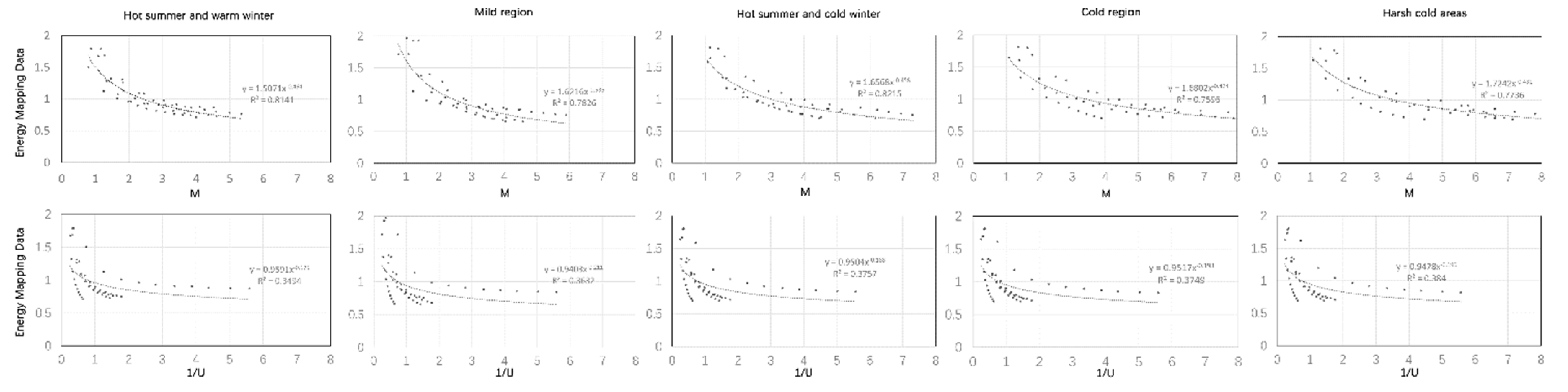
(b)

The correlation R² between comprehensive index and energy consumption was 0.7736–0.8215, which was approximately equal to twice the correlation of heat transfer coefficient, and it was scientific to use M as the index for building energy consumption prediction.

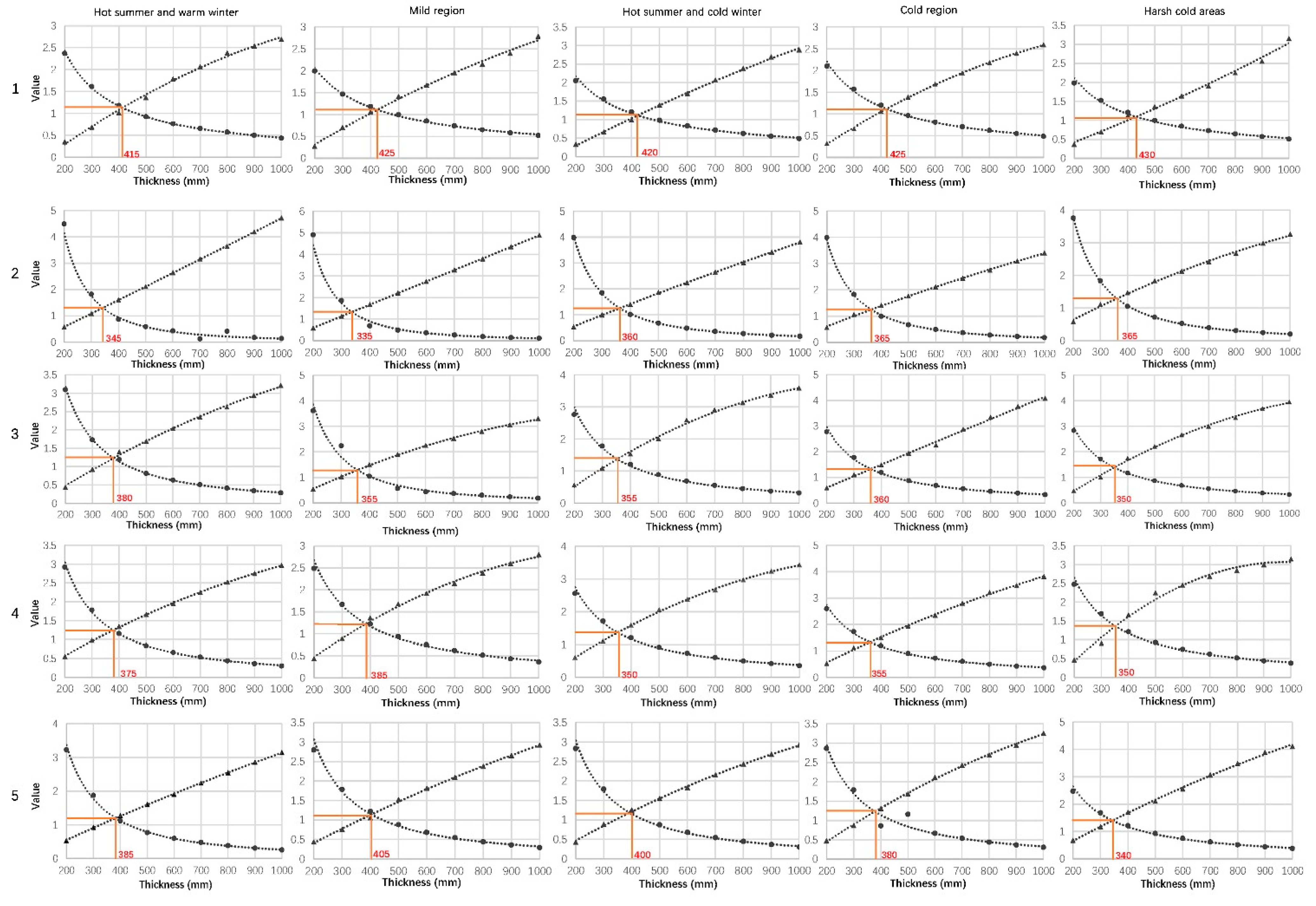
(c)

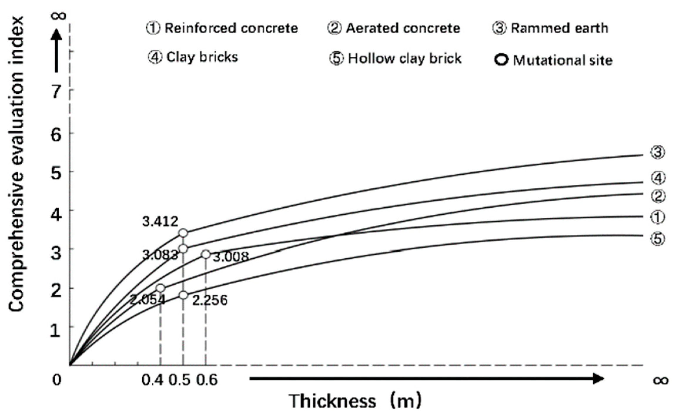
Using wall thickness as a general index, the correlation between the thermal performance of walls and building energy consumption was constructed and a balance between the two was sought; in addition, through numerical calculations and energy consumption simulations, the ideal wall thickness interval of five materials are shown in Table 22.

(d)

Considering the complex working conditions during practical construction, the conclusions of the paper provide a prospective application of the research: constructing the equivalence index between materials and transforming the single-material wall into a composite wall with a better performance, which is the direction the authors need to study subsequently.

Regardless of the foregoing, this study has the following limitations that need to be addressed in future research. First, the specific meaning of the balance point of the energy-saving rate and the thermal performance improvement rate must be explored and studied. Second, this paper uses five typical cities as research subjects in different climate zones; thus, the research object is not extensive, and later work needs to discuss more cities to verify whether the conclusions are universal.

References

1. Huo, T.F.; Ren, H.; Zhang, X.L.; Cai, W.G.; Feng, W.; Zhou, N.; Wang, X. China’s energy consumption in the building sector: A Statistical Yearbook-Energy Balance Sheet based splitting method. J. Clean. Prod. 2018, 185, 665–679. [Google Scholar] [CrossRef]
2. EIA. International Energy Outlook 2016. 2017. Available online: https://www.eia.gov/electricity/ (accessed on 14 December 2021).
3. Building Energy Conservation Research Center of Tsinghua University. Annual Report on the Development of Chinese Building Energy Efficiency 2018; China Building Industry Press: Beijing, China, 2018. (In Chinese) [Google Scholar]
4. Ministry of Housing and Urban-Rural Development of the People’s Republic of China (MOHURD). Design Code for Civil Building Energy Efficiency (JGJ 26-86); China Architecture & Building Press: Beijing, China, 1986. (In Chinese)
5. Ministry of Housing and Urban-Rural Development of the People’s Republic of China (MOHURD). Residential Buildings in Severe Cold and Cold Zones (JGJ 26-2018); China Architecture & Building Press: Beijing, China, 2018. (In Chinese)
6. Ministry of Housing and Urban-Rural Development of the People’s Republic of China (MOHURD). Design Standard for Energy Efficiency of Public Buildings (GB 50189-2015); China Architecture & Building Press: Beijing, China, 2015. (In Chinese)
7. Kaynakli, O. A review of the economical and optimum thermal insulation thickness for building applications. Renew. Sustain. Energy Rev. 2012, 16, 415–425. [Google Scholar] [CrossRef]
8. Dylewski, R.; Adamczyk, J. Study on ecological cost-effectiveness for the thermal insulation of building external vertical walls in Poland. Renew. Sustain. Energy Rev. 2012, 16, 415–425. [Google Scholar] [CrossRef]
9. Daouas, N. Impact of external longwave radiation on optimum insulation thickness in Tunisian building roofs based on a dynamic analytical model. Appl. Energy 2016, 177, 136–148. [Google Scholar] [CrossRef]
10. Song, X.Y.; Ye, C.T.; Li, H.S.; Wang, X.L.; Ma, W.B. Field study on energy economic assessment of office buildings envelope retrofitting in southern China. Sustain. Cities Soc. 2017, 28, 154–161. [Google Scholar] [CrossRef]
11. Zhang, L.L.; Li, Z.A.; Hou, C.P.; Wei, D.; Hou, Y.Y. Optimization analysis of thermal insulation layer attributes of building envelope exterior wall based on DeST and life cycle economic evaluation. Case Stud. Therm. Eng. 2019, 14, 100410. [Google Scholar] [CrossRef]
12. Dodoo, A.; Gustavsson, L.; Tettey, U.Y.A. Cost-optimized energy-efficient building envelope measures for a multi-story residential building in a cold climate. Energy Procedia 2019, 158, 3760–3767. [Google Scholar] [CrossRef]
13. Majumder, A.; Canale, L.; Mastino, C.C.; Pacitto, A.; Frattolillo, A.; Dell’Isola, M. Thermal Characterization of Recycled Materials for Building Insulation. Energies 2021, 14, 3564. [Google Scholar] [CrossRef]
14. Bellamy, L.A.; Mackenzie, D.W. Thermal Performance of Buildings with Heavy Walls; Technical report; BRANZ: Judgeford, New Zealand, 2001. [Google Scholar]
15. Zhu, L.; Hurt, R.; Correia, D.; Boehm, R. Detailed energy saving performance analyses on thermal mass walls demonstrated in a zero energy house. Energy Build. 2009, 41, 303–310. [Google Scholar] [CrossRef]
16. Ghoreishi, A.H.; Ali, M.M. Parametric study of thermal mass property of concrete buildings in U.S. climate zones. J. Archit. Sci. Rev. 2013, 56, 103–117. [Google Scholar] [CrossRef]
17. Al-Sanea, S.A.; Zedan, M.F.; Al-Hussain, S.N. Effect of thermal mass on the performance of insulated building walls and the concept of energy savings potential. Appl. Energy 2012, 89, 430–442. [Google Scholar] [CrossRef]
18. Dodoo, A.; Gustavsson, L.; Sathre, R. Effect of thermal mass on life cycle primary energy balances of a concrete-and a wood-frame building. Appl. Energy 2012, 92, 462–472. [Google Scholar] [CrossRef]
19. Wang, L.-S.; Ma, P.; Hu, E.; Giza-Sisson, D.; Mueller, G.; Guo, N. A study of building envelope and thermal mass requirements for achieving thermal autonomy in an office building. Energy Build. 2014, 78, 79–88. [Google Scholar] [CrossRef]
20. Reilly, A.; Kinnane, O. The impact of thermal mass on building energy consumption. Appl. Energy 2017, 198, 108–121. [Google Scholar] [CrossRef] [Green Version]
21. Deng, J.; Yao, R.; Yu, W.; Zhang, Q.; Li, B. Effectiveness of the thermal mass of external walls on residential buildings for part-time part-space heating and cooling using the state-space method. Energy Build. 2019, 190, 155–171. [Google Scholar] [CrossRef] [Green Version]
22. Hoes, P.; Trcka, M.; Hensen, J.L.M.; Bonnema, B.H. Investigating the potential of a novel low-energy house concept with hybrid adaptable thermal storage. Energy Convers. Manag. 2011, 52, 2442–2447. [Google Scholar] [CrossRef] [Green Version]
23. Hoes, P.; Hensen, J.L.M. The potential of lightweight low-energy houses with hybrid adaptable thermal storage: Comparing the performance of promising concepts. Energy Build. 2016, 110, 79–93. [Google Scholar] [CrossRef]
24. Bojić, M.; Loveday, D. The influence on building thermal behavior of the insulation/masonry distribution in a three-layered construction. Energy Build. 1997, 26, 153–157. [Google Scholar] [CrossRef]
25. Kossecka, E.; Kosny, J. Influence of insulation configuration on heating and cooling loads in a continuously used building. Energy Build. 2002, 34, 321–331. [Google Scholar] [CrossRef]
26. Van Hooff, T.; Blocken, B.; Timmermans, H.J.P.; Hensen, J.L.M. Analysis of the predicted effect of passive climate adaptation measures on energy demand for cooling and heating in a residential building. Energy 2016, 94, 811–820. [Google Scholar] [CrossRef]
27. Department for Communities and Local Government (UK). Building Regulations. Approved Document L: Conservation of Fuel and Power; Department for Communities and Local Government: London, UK, 2016.
28. Kinnane, O.; Sinnott, D.; Turner, W. Evaluation of passive ventilation provision in domestic housing retrofit. Build. Environ. 2016, 106, 205–218. [Google Scholar] [CrossRef]
29. Ministry of Housing and Urban-Rural Development of the People’s Republic of China (MOHURD). Code for Thermal Design of Civil Building (GB 50176-2016); China Architecture & Building Press: Beijing, China, 2016. (In Chinese) [Google Scholar]
30. National Bureau of Statistics of the People’Cs Republic of China. China Statistical Yearbook; China Statistics Press: Beijing, China, 2020. (In Chinese)
31. Ministry of Housing and Urban-Rural Development of the People’s Republic of China (MOHURD). Design Code for Heating Ventilation and Air Conditioning of Civil Buildings (GB50736-2012); China Architecture & Building Press: Beijing, China, 2012. (In Chinese)
Figure 1. Basic case model, three-dimensional image (top).
Sustainability 14 01143 g001
Figure 2. Diagram of temperature fluctuation interval inside the wall.
Sustainability 14 01143 g002
Figure 3. Thermal mass introduces a time lag.
Sustainability 14 01143 g003
Figure 4. Schematic diagram of MGZ.
Sustainability 14 01143 g004
Figure 5. Schematic diagram of MKM.
Sustainability 14 01143 g005
Figure 6. Schematic diagram of MSH.
Sustainability 14 01143 g006
Figure 7. Schematic diagram of MBJ.
Sustainability 14 01143 g007
Figure 8. Schematic diagram of MHRB.
Sustainability 14 01143 g008
Figure 9. Minimum temperature of the inner surface in Guangzhou.
Sustainability 14 01143 g009
Figure 10. Minimum temperature of the inner surface in Kunming.
Sustainability 14 01143 g010
Figure 11. Minimum temperature of the inner surface in Shanghai.
Sustainability 14 01143 g011
Figure 12. Minimum temperature of an inner surface in Beijing.
Sustainability 14 01143 g012
Figure 13. Minimum temperature of an inner surface in Harbin.
Sustainability 14 01143 g013
Figure 14. Different reference indicators and energy mapping data.
Sustainability 14 01143 g014
Figure 15. Improvement and energy-saving rate.
Sustainability 14 01143 g015
Figure 16. Establishment of equivalent composite index.
Sustainability 14 01143 g016