
A New Fractional-Order Load Frequency Control for Multi-Renewable Energy Interconnected Plants Using Skill Optimization Algorithm
 , ,
, ,  , and
, and
Abstract
:1. Introduction
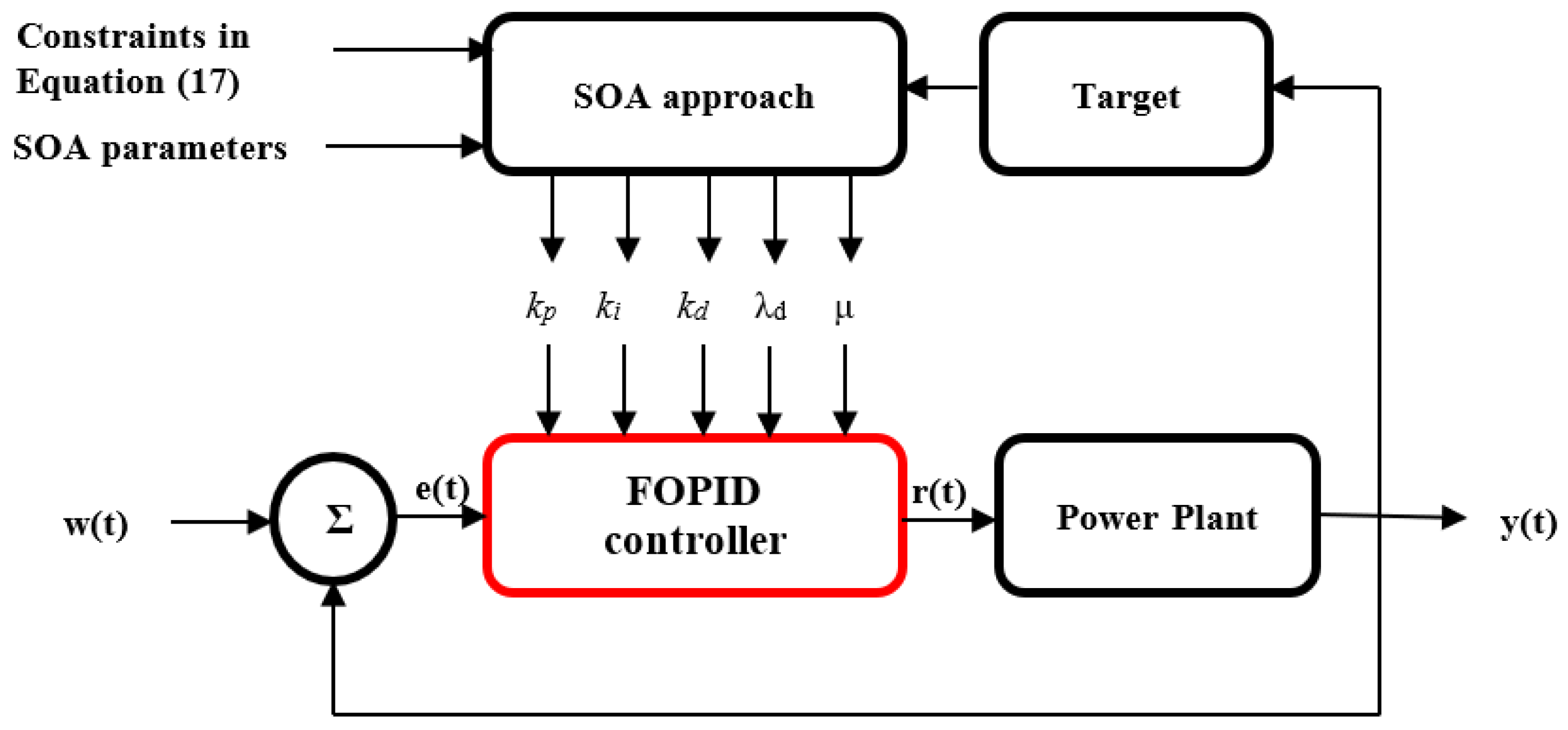
- A new skill optimization algorithm (SOA)-based methodology is proposed to design FOPID-LFC installed with interconnected systems with RESs.
- Two power systems are investigated, PV/thermal and thermal/wind turbine/thermal/PV, at different load disturbances.
- An extensive comparison of CBOA, JSOA, BO, TDO, and AOS is conducted.
- Statistical tests of Friedman ANOVA table, Wilcoxon rank test, Friedman rank test, and Kruskal Wallis test are implemented.
- The competence and reliability of the proposed SOA are confirmed via the obtained results.
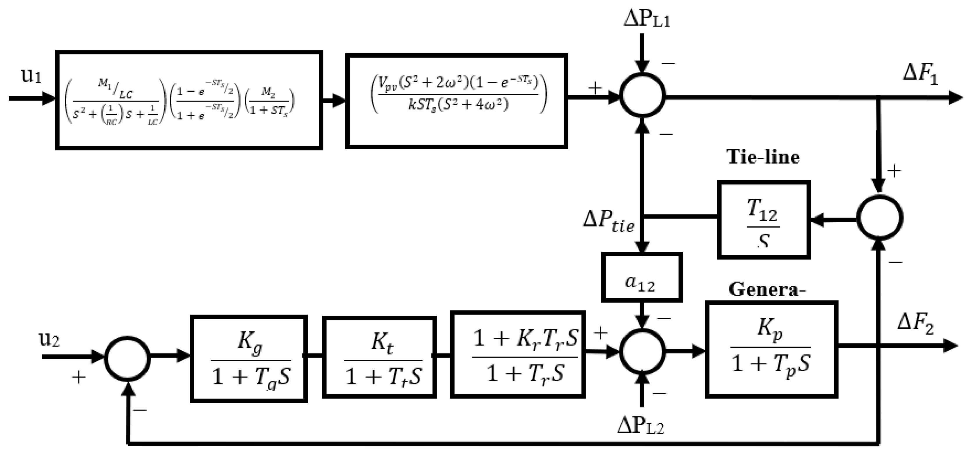
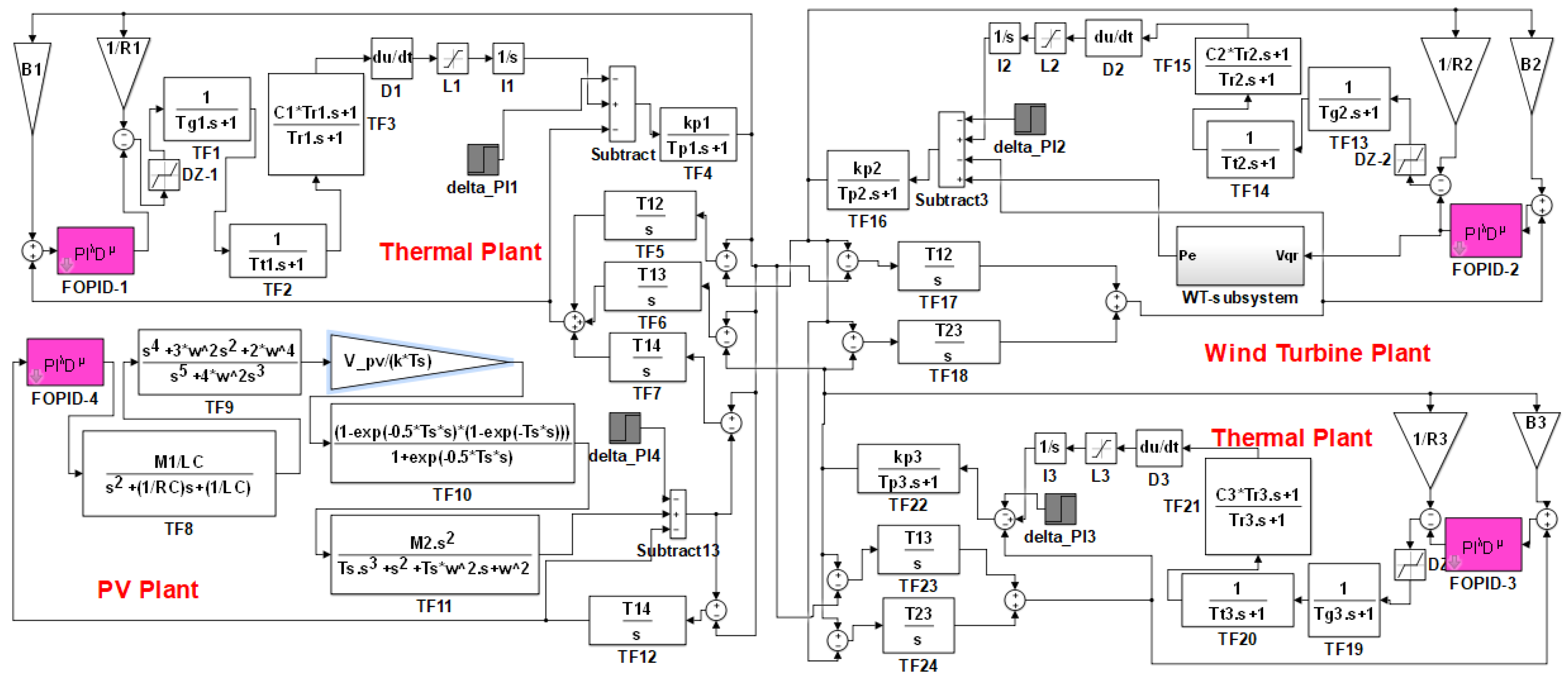
2. Model of Interconnected Systems
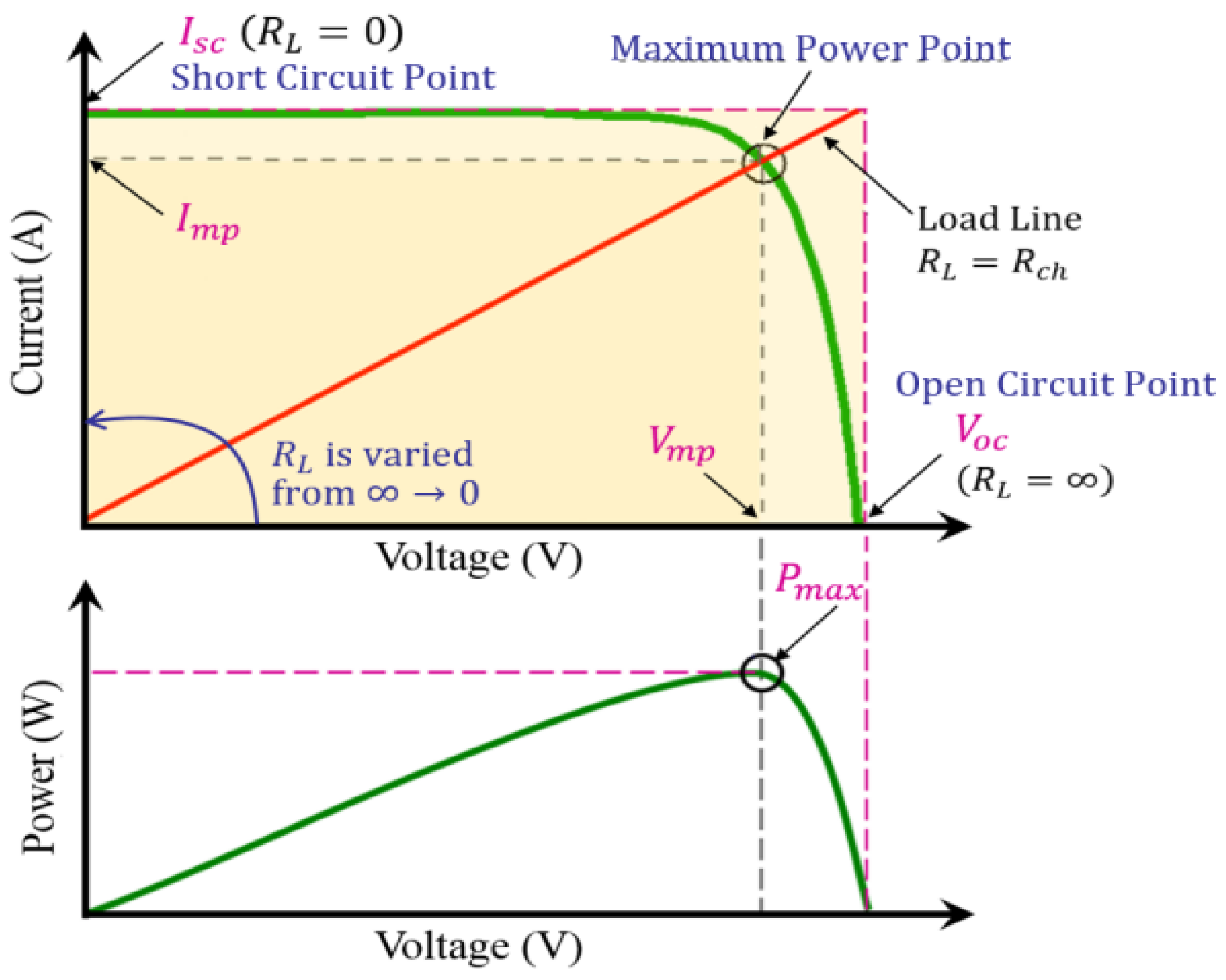
2.1. PV Plant Model
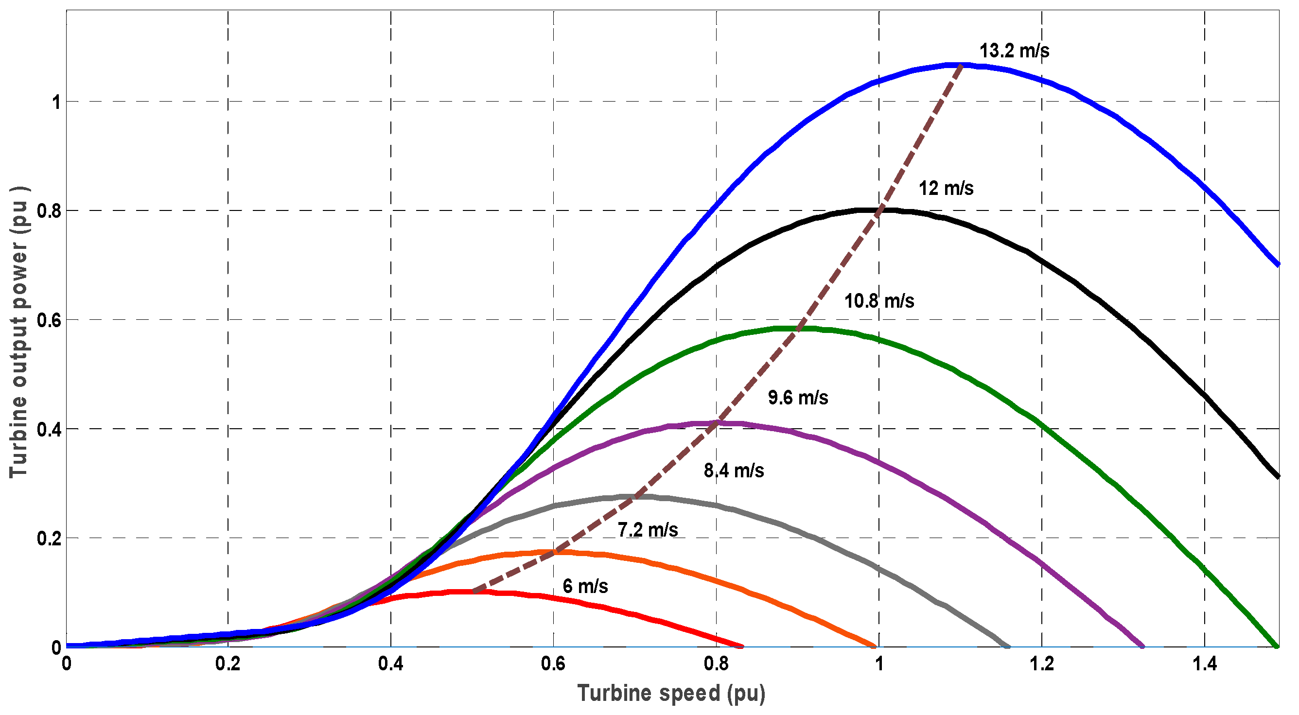
2.2. Model of WT
2.3. Thermal Plant Model
3. Fractional-Order PID Controller (FOPID)
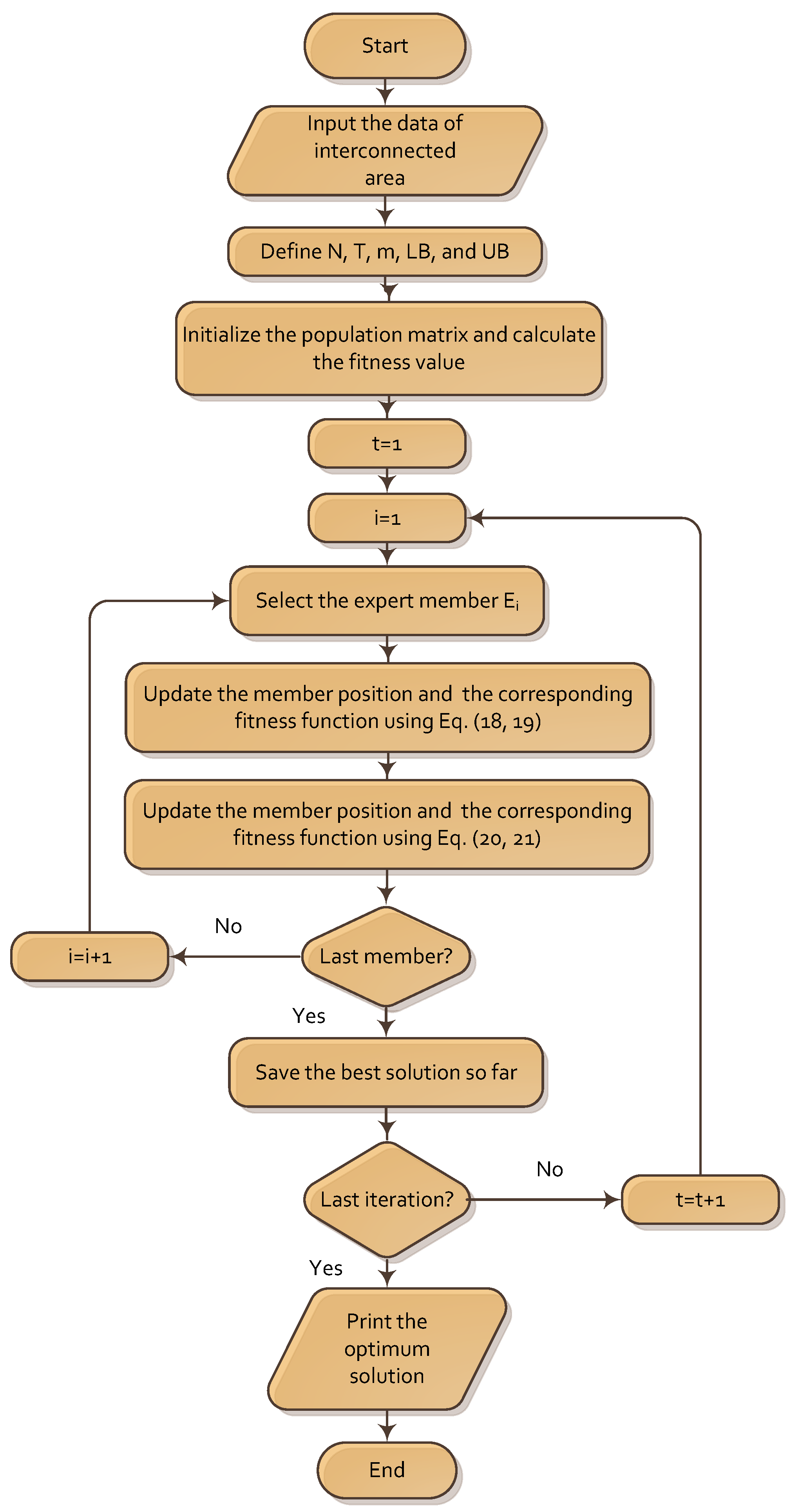
4. The Proposed Skill Optimization Algorithm
4.1. Exploration Phase
4.2. Exploitation Phase
5. The Proposed Optimization Problem
5.1. The Fitness Function
5.2. The SOA-Based Solution Methodology
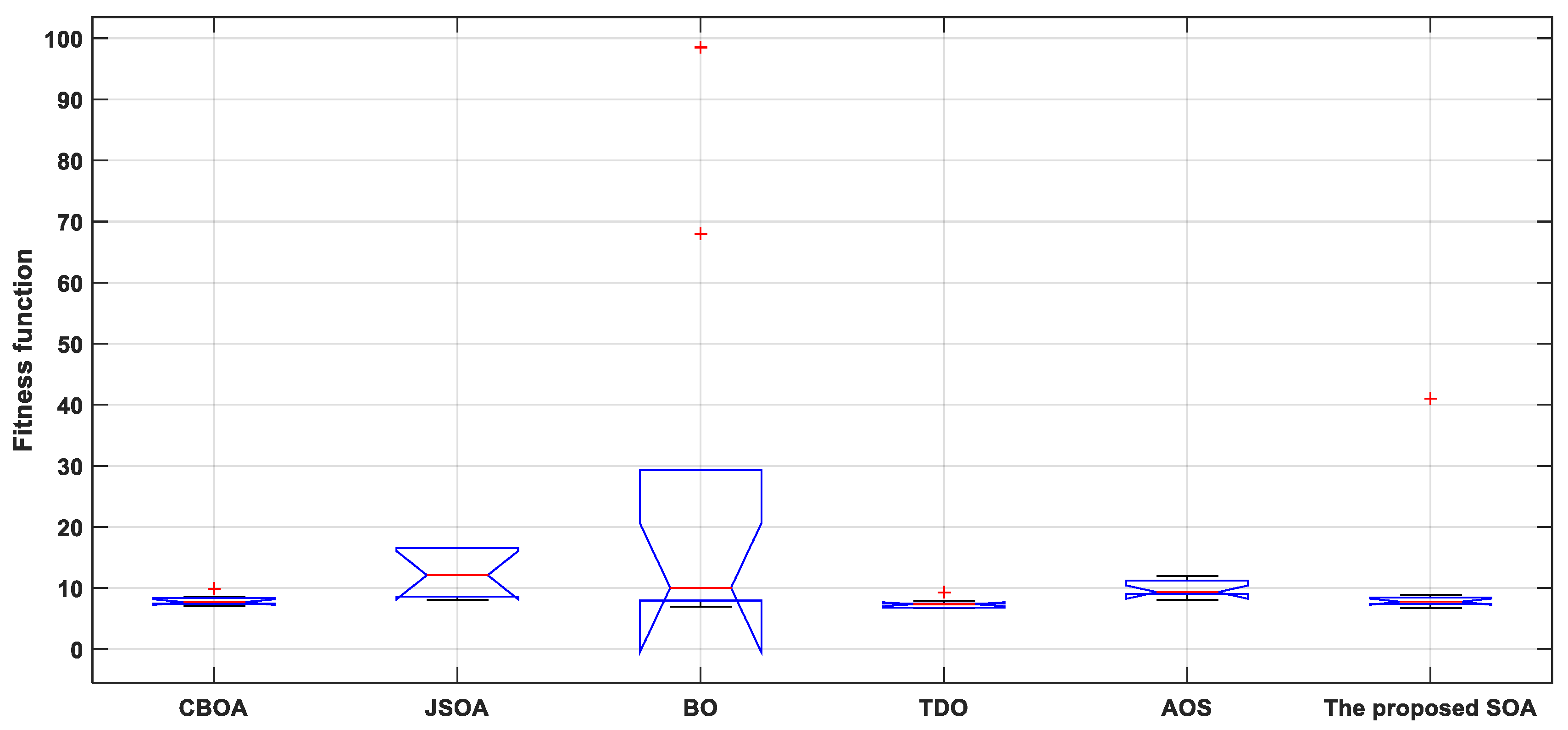
6. Numerical Analysis
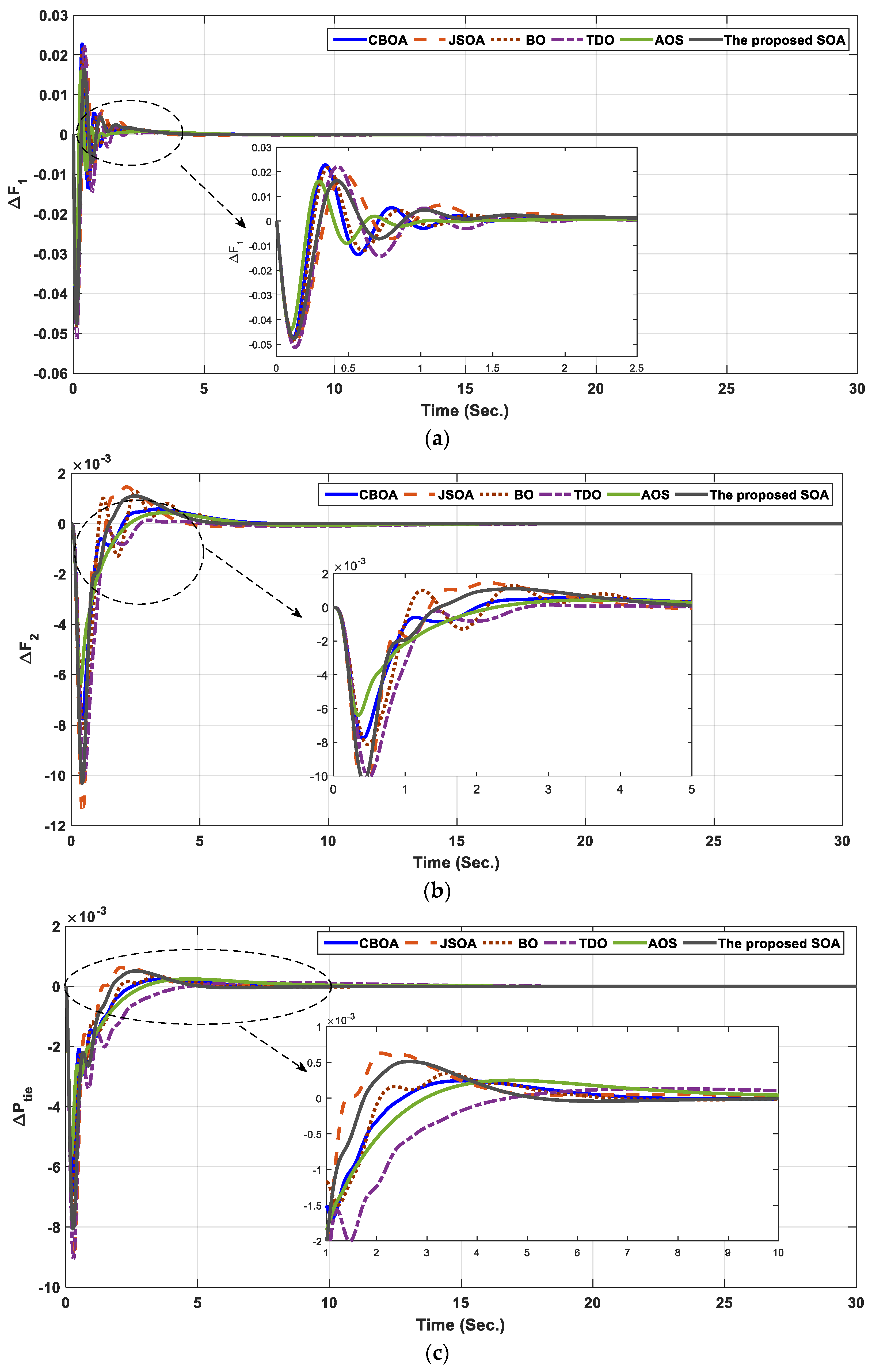
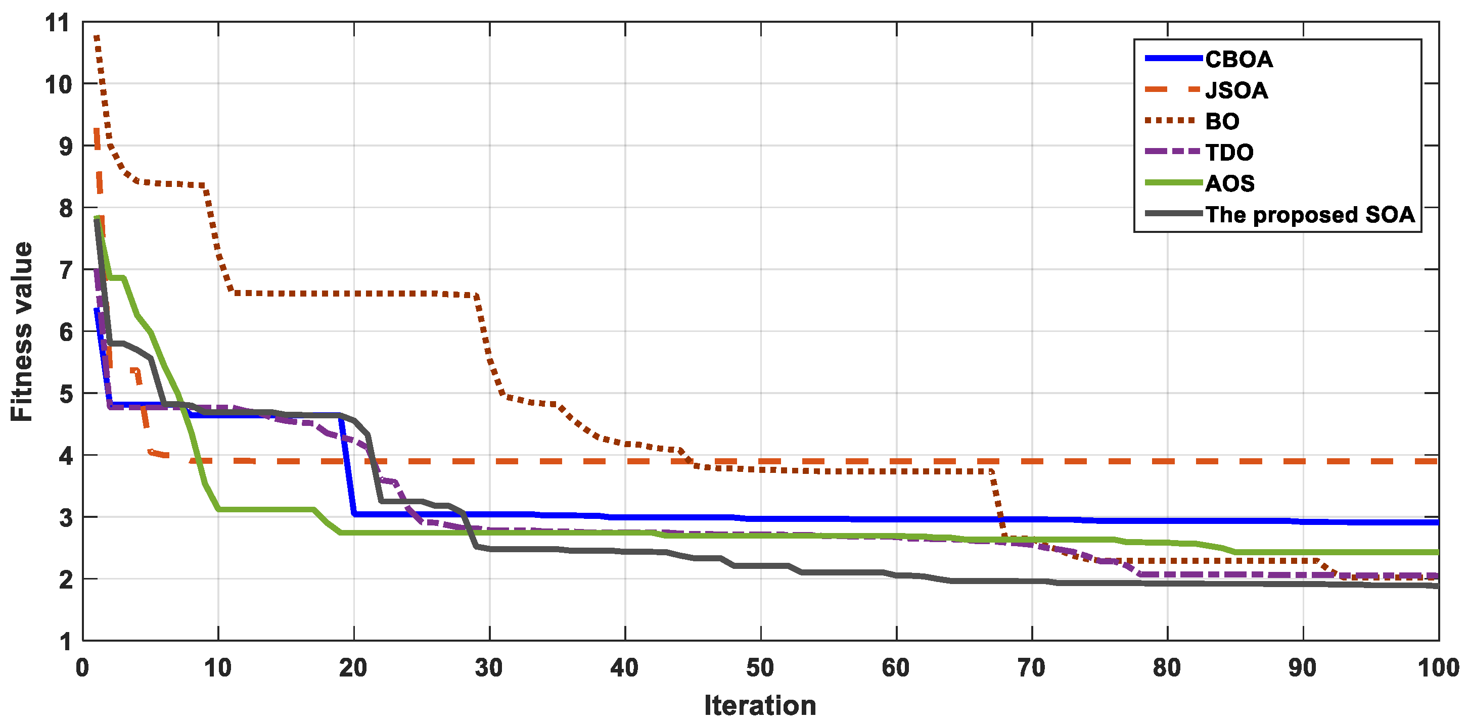
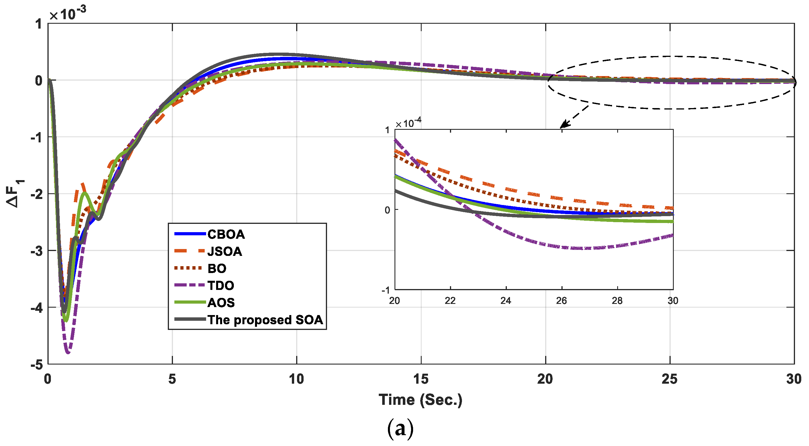
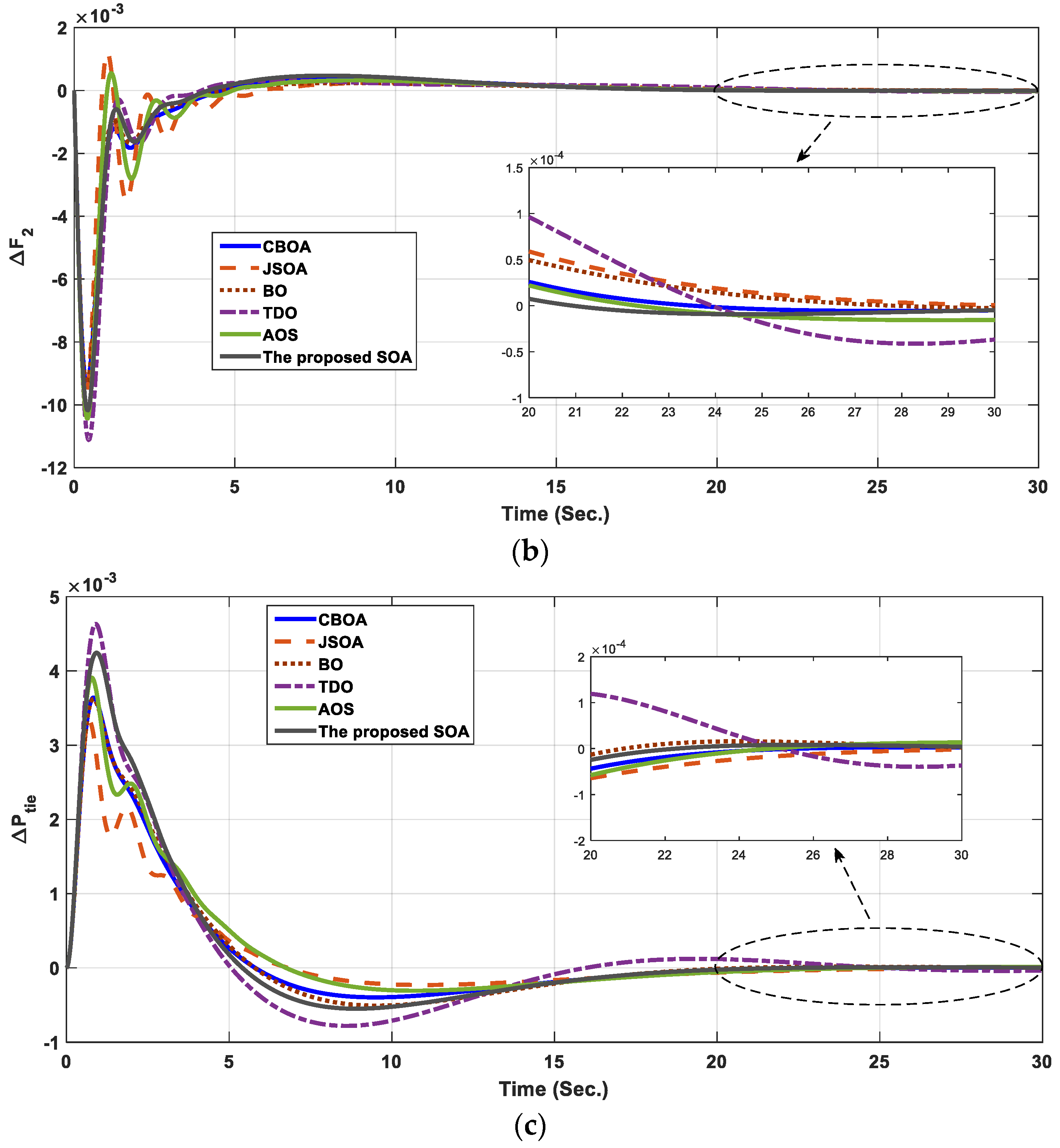
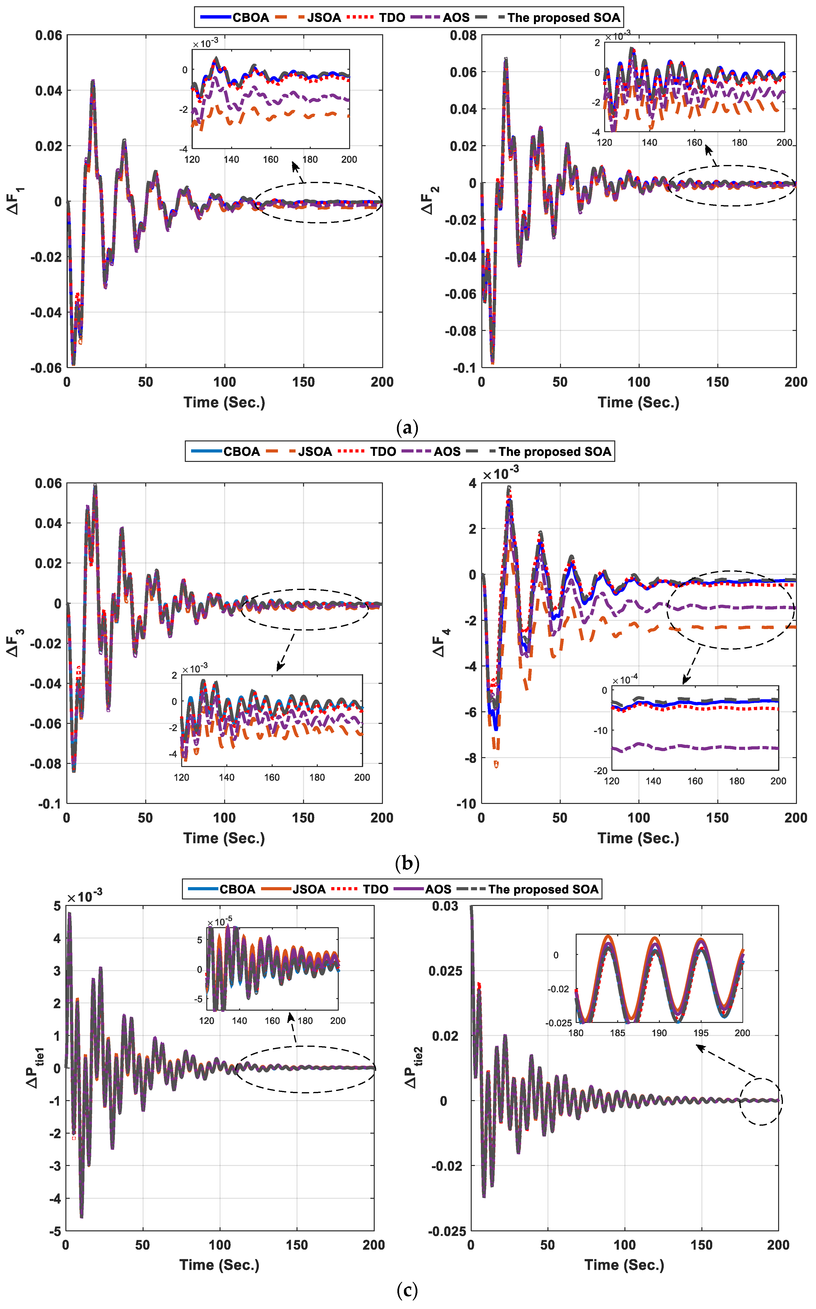
6.1. Two-Interconnected Power System
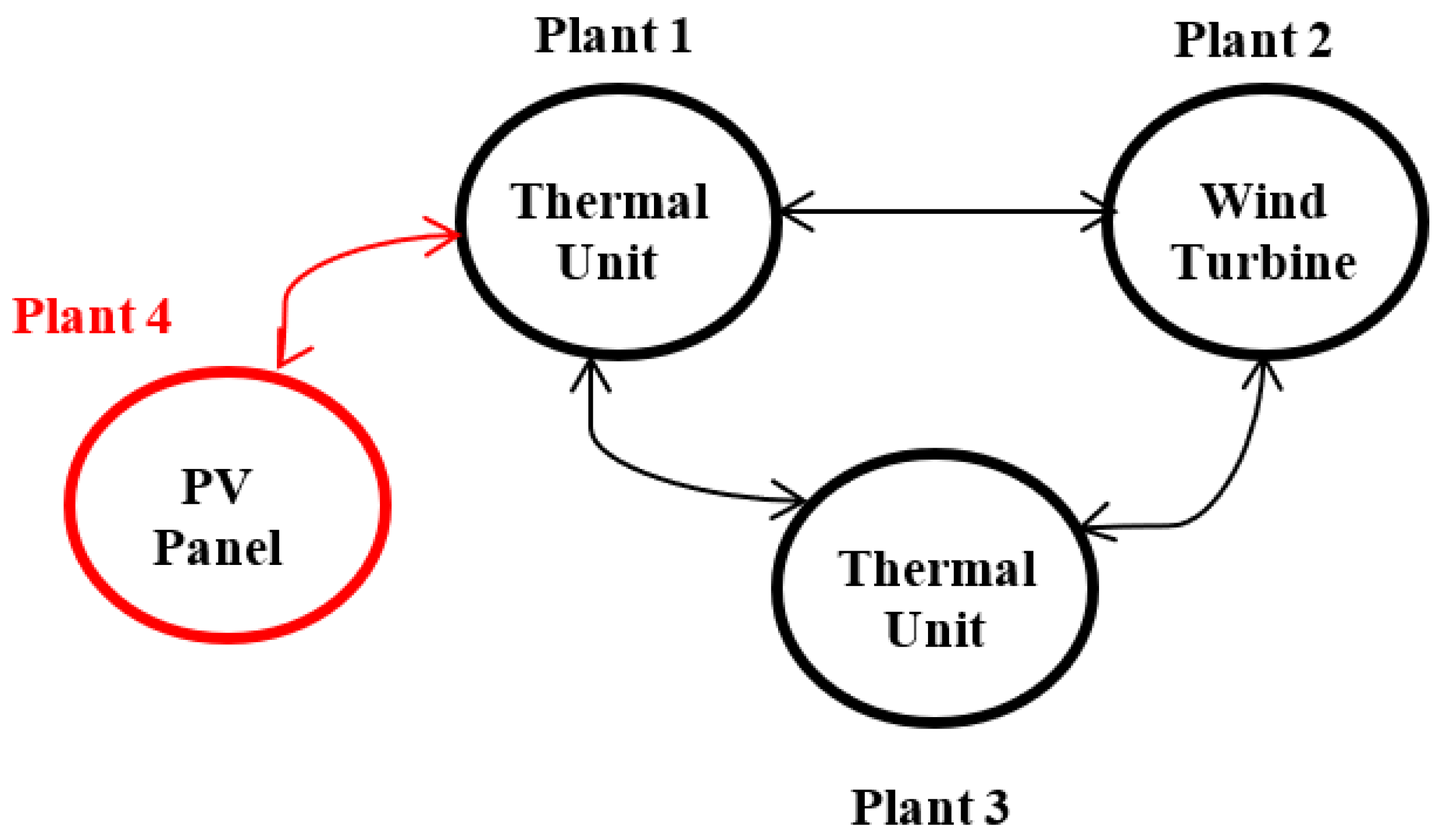
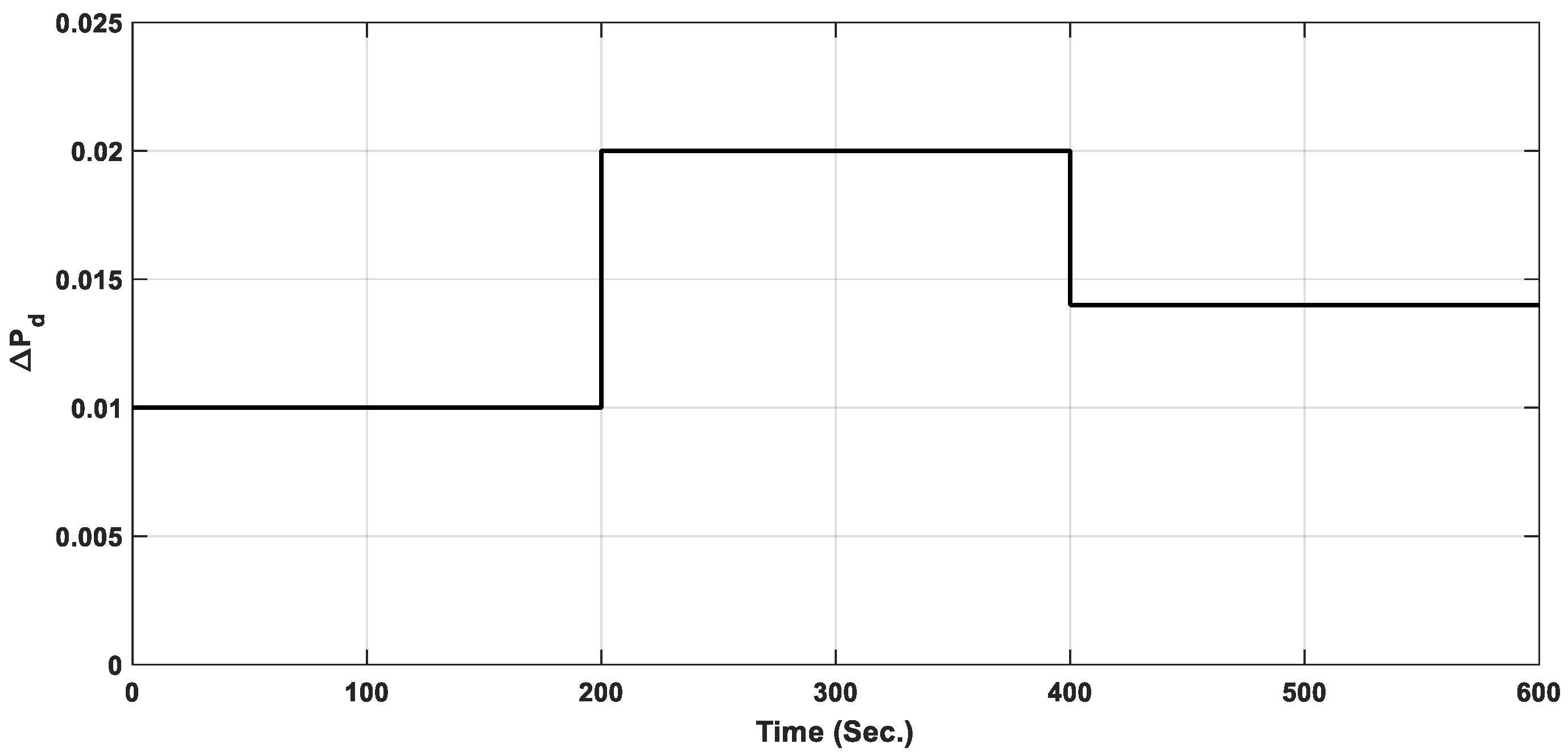
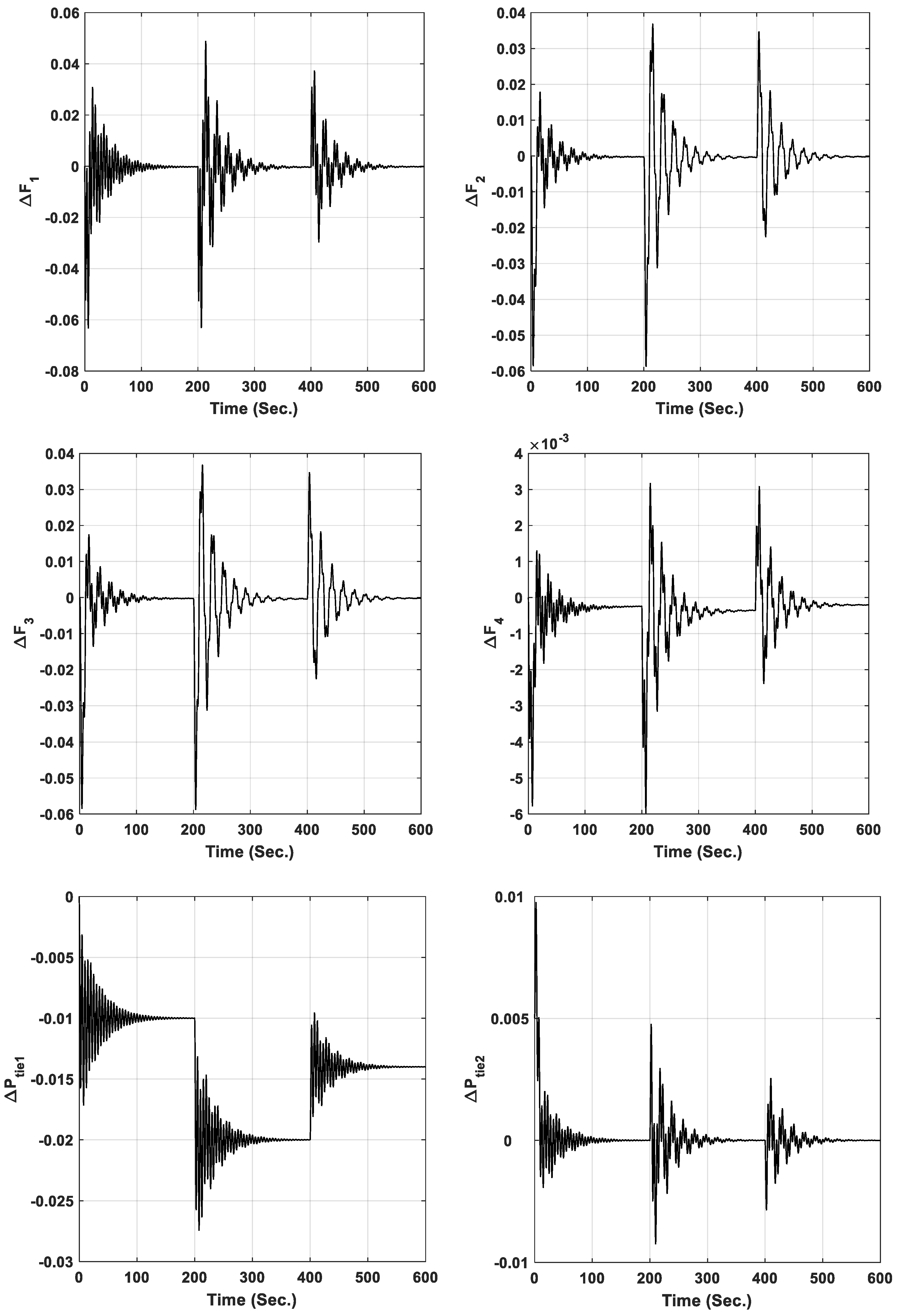
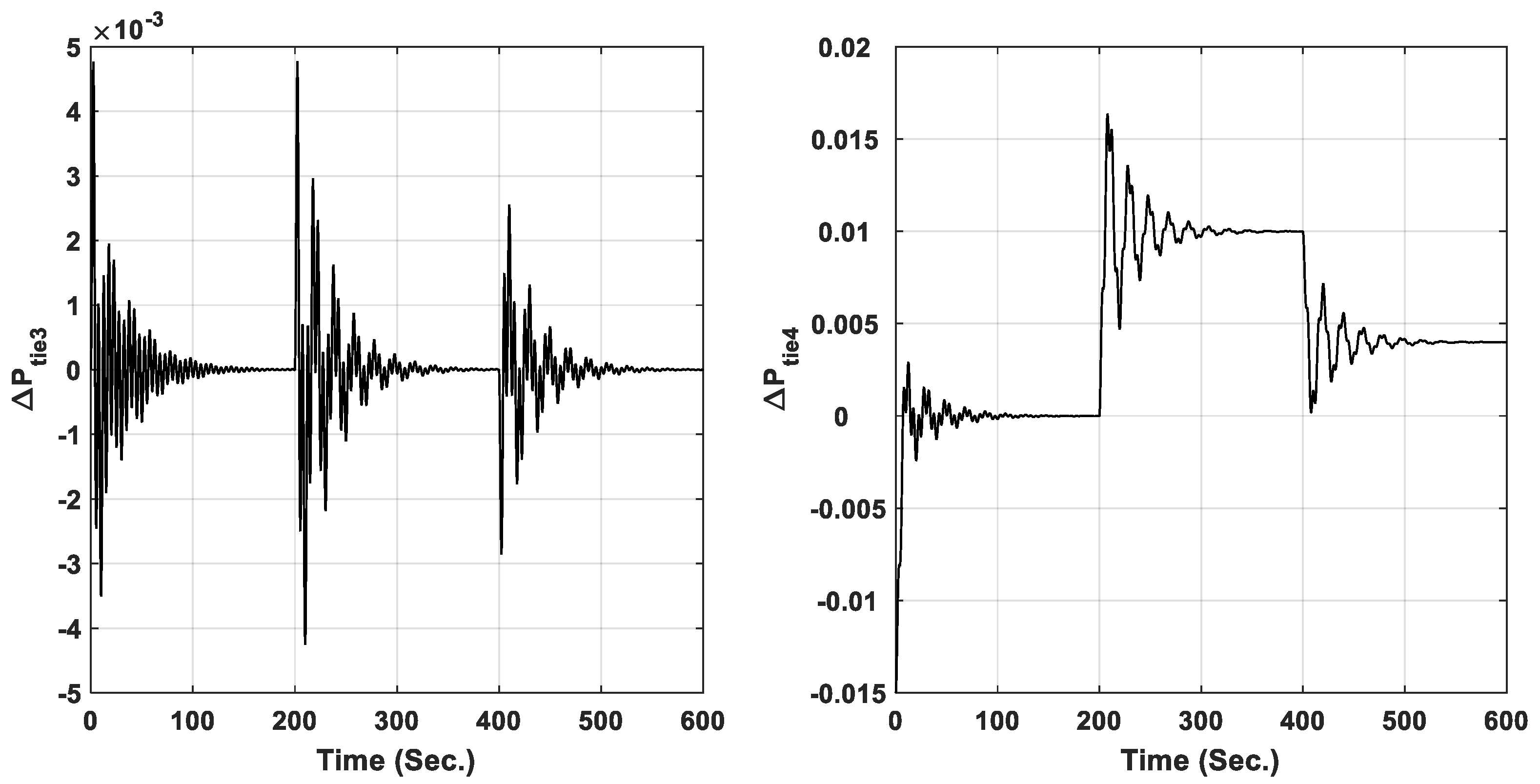
6.2. Four Interconnected Power System
7. Conclusions
Author Contributions
Funding
Institutional Review Board Statement
Informed Consent Statement
Data Availability Statement
Conflicts of Interest
Nomenclature
| PV panel output current | Radius of turbine | ||
| PV panel output voltage | Wind speed | ||
| Number of series cells | Air density | ||
| Number of parallel cells | Swept area of turbine blades | ||
| Factor of completion | Steam turbine transfer function | ||
| Boltzmann constant | Governor transfer function | ||
| PV panel temperature | Reheater transfer function | ||
| Electron charge | Generator transfer function | ||
| Irradiance in W/m2 | Steam turbine gain | ||
| Photo current | Governor gain | ||
| Saturation current | Reheater gain | ||
| Cell series resistance | Generator gain | ||
| PV module output power | Steam turbine time constant | ||
| Angular frequency of grid | Governor time constant | ||
| Converter output resistance | Reheater time constant | ||
| Converter output capacitance | Generator time constant | ||
| Converter output inductance | kp, ki, kd, λd, and μ | Parameters of FOPID controller | |
| Simulation time | , , and | Wind plant gains | |
| Buck converter voltage gain | , , and | Wind plant time constants | |
| Inverter converter voltage gain | FOPID controller input | ||
| Power coefficient | Violations in ith area frequency | ||
| λ | Tip ratio | Violations in ith area exchange power | |
| β | Pitch angle of blade | Specified time | |
| Mechanical angular speed of turbine | Number of interconnected plants |
References
- Shayeghi, H.; Shayanfar, H.; Jalili, A. Load frequency control strategies: A state-of-the-art survey for the researcher. Energy Convers. Manag. 2009, 50, 344–353. [Google Scholar] [CrossRef]
- Xu, D.; Liu, J.; Yan, X.-G.; Yan, W. A Novel Adaptive Neural Network Constrained Control for a Multi-Area Interconnected Power System With Hybrid Energy Storage. IEEE Trans. Ind. Electron. 2017, 65, 6625–6634. [Google Scholar] [CrossRef]
- Su, X.; Liu, X.; Song, Y.-D. Fault-Tolerant Control of Multiarea Power Systems via a Sliding-Mode Observer Technique. IEEE/ASME Trans. Mechatron. 2017, 23, 38–47. [Google Scholar] [CrossRef]
- Yousri, D.; Babu, T.S.; Fathy, A. Recent methodology based Harris Hawks optimizer for designing load frequency control incorporated in multi-interconnected renewable energy plants. Sustain. Energy Grids Netw. 2020, 22, 100352. [Google Scholar] [CrossRef]
- Ali, H.H.; Kassem, A.M.; Al-Dhaifallah, M.; Fathy, A. Multi-Verse Optimizer for Model Predictive Load Frequency Control of Hybrid Multi-Interconnected Plants Comprising Renewable Energy. IEEE Access 2020, 8, 114623–114642. [Google Scholar] [CrossRef]
- Fathy, A.; Alharbi, A.G. Recent Approach Based Movable Damped Wave Algorithm for Designing Fractional-Order PID Load Frequency Control Installed in Multi-Interconnected Plants With Renewable Energy. IEEE Access 2021, 9, 71072–71089. [Google Scholar] [CrossRef]
- Datta, A.; Bhattacharjee, K.; Debbarma, S.; Kar, B. Load frequency control of a renewable energy sources based hybrid system. In Proceedings of the 2015 IEEE Conference on Systems, Process and Control (ICSPC), Bandar Sunway, Malaysia, 18–20 December 2015; pp. 34–38. [Google Scholar] [CrossRef]
- Ramesh, M.; Yadav, A.K.; Pathak, P.K. An extensive review on load frequency control of solar-wind based hybrid renewable energy systems. Energy Sources Part A Recover. Util. Environ. Eff. 2021, 1–25. [Google Scholar] [CrossRef]
- Fathy, A.; Kassem, A.M. Antlion optimizer-ANFIS load frequency control for multi-interconnected plants comprising photovoltaic and wind turbine. ISA Trans. 2019, 87, 282–296. [Google Scholar] [CrossRef]
- Ranjan, M.; Shankar, R. A literature survey on load frequency control considering renewable energy integration in power system: Recent trends and future prospects. J. Energy Storage 2022, 45, 103717. [Google Scholar] [CrossRef]
- Magdy, G.; Bakeer, A.; Alhasheem, M. Robust decentralized model predictive load-frequency control design for time-delay renewable power systems. Int. J. Emerg. Electr. Power Syst. 2021, 22, 617–628. [Google Scholar] [CrossRef]
- El-Ela, A.A.A.; El-Sehiemy, R.A.; Shaheen, A.M.; Diab, A.E.-G. Design of cascaded controller based on coyote optimizer for load frequency control in multi-area power systems with renewable sources. Control Eng. Pract. 2022, 121, 105058. [Google Scholar] [CrossRef]
- Arora, K.; Kumar, A.; Kamboj, V.K.; Prashar, D.; Shrestha, B.; Joshi, G.P. Impact of Renewable Energy Sources into Multi Area Multi-Source Load Frequency Control of Interrelated Power System. Mathematics 2021, 9, 186. [Google Scholar] [CrossRef]
- Gulzar, M.M.; Iqbal, M.; Shahzad, S.; Muqeet, H.A.; Shahzad, M.; Hussain, M.M. Load Frequency Control (LFC) Strategies in Renewable Energy-Based Hybrid Power Systems: A Review. Energies 2022, 15, 3488. [Google Scholar] [CrossRef]
- Latif, A.; Suhail Hussain, S.M.; Das, D.C.; Ustun, T.S. State-of-the-art of controllers and soft computing techniques for regulated load frequency management of single/multi-area traditional and renewable energy based power systems. Appl. Energy 2020, 266, 114858. [Google Scholar] [CrossRef]
- Tungadio, D.H.; Sun, Y. Load frequency controllers considering renewable energy integration in power system. Energy Rep. 2019, 5, 436–453. [Google Scholar] [CrossRef]
- Pandey, S.K.; Mohanty, S.R.; Kishor, N. A literature survey on load–frequency control for conventional and distribution generation power systems. Renew. Sustain. Energy Rev. 2013, 25, 318–334. [Google Scholar] [CrossRef]
- Takayama, S.; Matsuhashi, R. Development of model for load frequency control in power system with large-scale integration of renewable energy. In Proceedings of the 2016 IEEE Power and Energy Conference at Illinois (PECI), Urbana, IL, USA, 19–20 February 2016; pp. 1–8. [Google Scholar] [CrossRef]
- Khalid, J.; Ramli, M.A.; Khan, M.S.; Hidayat, T. Efficient Load Frequency Control of Renewable Integrated Power System: A Twin Delayed DDPG-Based Deep Reinforcement Learning Approach. IEEE Access 2022, 10, 51561–51574. [Google Scholar] [CrossRef]
- Sobhy, M.A.; Abdelaziz, A.Y.; Hasanien, H.M.; Ezzat, M. Marine predators algorithm for load frequency control of modern interconnected power systems including renewable energy sources and energy storage units. Ain Shams Eng. J. 2021, 12, 3843–3857. [Google Scholar] [CrossRef]
- El-Ela, A.A.A.; El-Sehiemy, R.A.; Shaheen, A.M.; Diab, A.E.-G. Enhanced coyote optimizer-based cascaded load frequency controllers in multi-area power systems with renewable. Neural Comput. Appl. 2021, 33, 8459–8477. [Google Scholar] [CrossRef]
- Subham, G.T.; Ramachandran, R.; Kandasamy, J.; Muralidharan, R. Automatic Load Frequency Control of Renewable Energy Integrated Hybrid Power System. J. Trends Comput. Sci. Smart Technol. 2022, 4, 10–16. [Google Scholar] [CrossRef]
- Abhilash, T.; Pavani, A.P. Multi area load frequency control of power system involving renewable and non-renewable energy sources. In Proceedings of the 2017 Innovations in Power and Advanced Computing Technologies (i-PACT), Vellore, India, 21–22 April 2017; pp. 1–5. [Google Scholar] [CrossRef]
- Munisamy, V.; Sundarajan, R.S. Hybrid technique for load frequency control of renewable energy sources with unified power flow controller and energy storage integration. Int. J. Energy Res. 2021, 45, 17834–17857. [Google Scholar] [CrossRef]
- Masuta, T.; Shimizu, K.; Yokoyama, A. Load Frequency Control by use of a Number of Both Heat Pump Water Heaters and Electric Vehicles in Power System with a Large Integration of Renewable Energy Sources. IEEJ Trans. Power Energy 2012, 132, 23–33. [Google Scholar] [CrossRef]
- Dutta, A.; Prakash, S. Utilizing Electric Vehicles and Renewable Energy Sources for Load Frequency Control in Deregulated Power System Using Emotional Controller. IETE J. Res. 2022, 68, 1500–1511. [Google Scholar] [CrossRef]
- Hasanien, H.; El-Fergany, A. Salp swarm algorithm-based optimal load frequency control of hybrid renewable power systems with communication delay and excitation cross-coupling effect. Electr. Power Syst. Res. 2019, 176, 105938. [Google Scholar] [CrossRef]
- Huynh, V.; Minh, B.; Amaefule, E.; Tran, A.-T.; Tran, P. Highly Robust Observer Sliding Mode Based Frequency Control for Multi Area Power Systems with Renewable Power Plants. Electronics 2021, 10, 274. [Google Scholar] [CrossRef]
- Irudayaraj, A.X.R.; Wahab, N.I.A.; Premkumar, M.; Radzi, M.A.M.; Bin Sulaiman, N.; Veerasamy, V.; Farade, R.A.; Islam, M.Z. Renewable sources-based automatic load frequency control of interconnected systems using chaotic atom search optimization. Appl. Soft Comput. 2022, 119, 108574. [Google Scholar] [CrossRef]
- Rawat, S.; Jha, B.; Panda, M.K.; Rath, B.B. Load frequency control of a renewable hybrid power system with simple fuzzy logic controller. In Proceedings of the 2016 International Conference on Computing, Communication and Automation (ICCCA), Greater Noida, India, 29–30 April 2016; pp. 918–923. [Google Scholar] [CrossRef]
- Guha, D.; Roy, P.K.; Banerjee, S. Equilibrium optimizer-tuned cascade fractional-order 3DOF-PID controller in load frequency control of power system having renewable energy resource integrated. Int. Trans. Electr. Energy Syst. 2021, 31, e12702. [Google Scholar] [CrossRef]
- Saxena, A.; Shankar, R. Improved load frequency control considering dynamic demand regulated power system integrating renewable sources and hybrid energy storage system. Sustain. Energy Technol. Assess. 2022, 52, 102245. [Google Scholar] [CrossRef]
- Xu, Y.; Li, C.; Wang, Z.; Zhang, N.; Peng, B. Load Frequency Control of a Novel Renewable Energy Integrated Micro-Grid Containing Pumped Hydropower Energy Storage. IEEE Access 2018, 6, 29067–29077. [Google Scholar] [CrossRef]
- Barisal, A. Comparative performance analysis of teaching learning based optimization for automatic load frequency control of multi-source power systems. Int. J. Electr. Power Energy Syst. 2015, 66, 67–77. [Google Scholar] [CrossRef]
- Tedesco, F.; Casavola, A. Load/Frequency Control in the presence of Renewable Energy Systems: A Reference-Offset Governor approach. IFAC-PapersOnLine 2020, 53, 12548–12553. [Google Scholar] [CrossRef]
- Ahin, M.E.; Blaabjerg, F. A hybrid PV-battery/supercapacitor system and a basic active power control proposal in MATLAB/simulink. Electronics 2020, 9, 129. [Google Scholar]
- Ahin, M.E.; Okumuş, H.İ. Parallel-Connected Buck–Boost Converter with FLC for Hybrid Energy System. Electr. Power Compon. Syst. 2021, 48, 2117–2129. [Google Scholar]
- Walker, G. Evaluating MPPT converter topologies using a MATLAB PV model. J. Electr. Electron. Eng. Aust. 2001, 21, 49–55. [Google Scholar]
- Ahin, M.E.; Okumuş, H.İ. Physical structure, electrical design, mathematical modeling and simulation of solar cells and modules. Turk. J. Electromech. Energy 2016, 1. [Google Scholar] [CrossRef]
- Mustafa, E.Ž.; Adel, M.S.; Halil, O. A novel filter compensation scheme for single phase-self-excited induction generator micro wind generation system. Sci. Res. Essays 2012, 7, 3058–3072. [Google Scholar]
- Renaudineau, H.; Donatantonio, F.; Fontchastagner, J.; Petrone, G.; Spagnuolo, G.; Martin, J.-P.; Pierfederici, S. A PSO-Based Global MPPT Technique for Distributed PV Power Generation. IEEE Trans. Ind. Electron. 2014, 62, 1047–1058. [Google Scholar] [CrossRef]
- Adly, M.; Besheer, A. A meta-heuristics search algorithm as a solution for energy transfer maximization in stand-alone photovoltaic systems. Int. J. Electr. Power Energy Syst. 2013, 51, 243–254. [Google Scholar] [CrossRef]
- Alam, M.K.; Khan, F.H. Transfer function mapping for a grid connected PV system using reverse synthesis technique. In Proceedings of the 2013 IEEE 14th Workshop on Control and Modeling for Power Electronics (COMPEL), Salt Lake City, UT, USA, 23–26 June 2013; pp. 1–5. [Google Scholar] [CrossRef]
- Kassem, A.M.; Abdelaziz, A.Y. Reactive power control for voltage stability of standalone hybrid wind–diesel power system based on functional model predictive control. IET Renew. Power Gener. 2014, 8, 887–899. [Google Scholar] [CrossRef]
- Kassem, A.M.; Yousef, A.M. Voltage and frequency control of an autonomous hybrid generation system based on linear model predictive control. Sustain. Energy Technol. Assess. 2013, 4, 52–61. [Google Scholar] [CrossRef]
- Chekkal, S.; Lahaçani, N.A.; Aouzellag, D.; Ghedamsi, K. Fuzzy logic control strategy of wind generator based on the dual-stator induction generator. Int. J. Electr. Power Energy Syst. 2014, 59, 166–175. [Google Scholar] [CrossRef]
- Sahu, R.K.; Gorripotu, T.S.; Panda, S. A hybrid DE–PS algorithm for load frequency control under deregulated power system with UPFC and RFB. Ain Shams Eng. J. 2015, 6, 893–911. [Google Scholar] [CrossRef] [Green Version]
- Santy, T.; Natesan, R. Load frequency control of a two area system consisting of a grid connected PV system and diesel generator. Int. J. Emerg. Technol. Comput. Electron. 2015, 13, 456–461. [Google Scholar]
- Podlubny, I. Fractional-order systems and fractional-order controllers. Inst. Exp. Phys. Slovak Acad. Sci. Kosice 1994, 12, 1–18. [Google Scholar]
- Givi, H.; Marie, H. Skill optimization algorithm: A new human-based metaheuristic technique. Comput. Mater. Contin. 2022, 74, 179–202. [Google Scholar] [CrossRef]
- Sahu, B.K.; Pati, S.; Panda, S. Hybrid differential evolution particle swarm optimisation optimised fuzzy proportional–integral derivative controller for automatic generation control of interconnected power system. IET Gener. Transm. Distrib. 2014, 8, 1789–1800. [Google Scholar] [CrossRef]


| CBOA | JSOA | BO | TDO | AOS | SOA | |
|---|---|---|---|---|---|---|
| kp1 | 1.0000 | 1.0000 | 1.0000 | 0.99998 | 1.0000 | 1.0000 |
| ki1 | 1.0000 | 1.0000 | 1.0000 | 0.48677 | 0.97191 | 0.9971 |
| kd1 | 1.0000 | 1.0000 | 1.0000 | 1.0000 | 1.0000 | 1.0000 |
| λd1 | 0.7725 | 0.23273 | 0.64308 | 0.33975 | 0.98977 | 0.35946 |
| μ1 | 0.65477 | 1.0000 | 0.69726 | 0.83521 | 0.65565 | 0.87552 |
| kp2 | 1.0000 | 1.0000 | 1.0000 | 0.26872 | 0.99882 | 0.99059 |
| ki2 | 1.0000 | 1.0000 | 1.0000 | 0.99909 | 1.0000 | 0.8911 |
| kd2 | 0.22547 | 1.0000 | 0.086092 | 0.99938 | 1.0000 | 0.13447 |
| λd2 | 0.53196 | 1.0000 | 0.00000 | 0.20817 | 1.0000 | 0.87058 |
| μ2 | 0.83065 | 1.0000 | 0.53543 | 0.77218 | 1.0000 | 0.977 |
| Elapsed time (Sec.) | 8924.533 | 3868.488 | 4265.285 | 6622.671 | 4707.0259 | 8151.158 |
| Fitness value | 7.1173 | 8.0539 | 6.9705 | 6.7558 | 8.0943 | 6.7506 |
| CBOA | JSOA | BO | TDO | AOS | SOA | |
|---|---|---|---|---|---|---|
| Best | 7.1173 | 8.0539 | 6.9705 | 6.6985 | 8.0943 | 6.7506 |
| Worst | 9.8586 | 16.552 | 98.501 | 9.2745 | 11.947 | 40.980 |
| Mean | 7.9378 | 12.403 | 26.497 | 7.4199 | 9.8271 | 11.064 |
| Median | 7.6988 | 12.107 | 10.046 | 7.3483 | 9.3298 | 7.7636 |
| Variance | 0.6422 | 16.461 | 994.99 | 0.5719 | 1.8280 | 1.1083 |
| Std. dev. | 0.8013 | 4.0572 | 31.544 | 0.7562 | 1.3520 | 0.5277 |
| CBOA | JSOA | BO | TDO | AOS | SOA | ||
|---|---|---|---|---|---|---|---|
| Wilcoxon rank test | p-value | 0.7913 | 0.0090 | 0.1405 | 0.1212 | 0.0073 | - |
| h-value | 0 | 1 | 0 | 0 | 1 | - | |
| Null hypothesis rejection | × | √ | × | × | √ | - | |
| Friedman rank | 4.4 | 9.6 | 8.1 | 5.0 | 8.7 | 3.2 | |
| Friedman test p-value | 6.8140e-05 | ||||||
| p-value based on ANOVA | 0.0308 | ||||||
| p-value based on Kruskal Wallis test | 1.3583e-04 | ||||||
| CBOA | JSOA | BO | TDO | AOS | SOA | |
|---|---|---|---|---|---|---|
| kp1 | 0.36569 | 0.1000 | 0.1000 | 0.10003 | 0.11668 | 0.1001 |
| ki1 | 0.1 | 1.0000 | 0.1000 | 0.10485 | 0.10334 | 0.1 |
| kd1 | 0.3708 | 0.1000 | 0.71061 | 0.99984 | 0.11471 | 0.14113 |
| λd1 | 0.8262 | 1.0000 | 0.61687 | 0.67797 | 0.72813 | 0.20952 |
| μ1 | 0.92171 | 0.90165 | 0.99761 | 0.94303 | 0.96683 | 0.78574 |
| kp2 | 0.87133 | 1.0000 | 0.99612 | 0.20311 | 0.11802 | 0.39052 |
| ki2 | 1.0000 | 1.0000 | 1.0000 | 0.99984 | 0.99783 | 1.0000 |
| kd2 | 1.0000 | 1.0000 | 1.0000 | 0.99577 | 0.96641 | 1.0000 |
| λd2 | 0.28196 | 1.0000 | 0.2517 | 0.10308 | 0.96431 | 0.28383 |
| μ2 | 0.95274 | 0.1000 | 0.99088 | 0.87324 | 0.11028 | 0.73404 |
| Fitness value | 2.9092 | 3.8959 | 2.0181 | 2.0489 | 2.4266 | 1.8779 |
| CBOA | JSOA | BO | TDO | AOS | SOA | |
|---|---|---|---|---|---|---|
| kp1 | 0.030335 | 0.015797 | 1.0000 | 0.01 | 0.013113 | 0.027242 |
| ki1 | 0.013487 | 0.020344 | 0.010001 | 0.102469 | 0.150434 | 0.014646 |
| kd1 | 0.01 | 0.01 | 0.0100 | 0.01 | 0.033762 | 0.032416 |
| λd1 | 0.016799 | 0.01 | 0.999969 | 0.010007 | 0.0100 | 0.031366 |
| μ1 | 0.033807 | 0.01 | 0.010001 | 0.01 | 0.0100 | 0.03194 |
| kp2 | 0.054376 | 0.01 | 0.278846 | 0.010621 | 0.059971 | 0.024249 |
| ki2 | 0.014237 | 0.01 | 0.253138 | 0.029362 | 0.0100 | 0.032453 |
| kd2 | 0.010332 | 0.064301 | 0.066672 | 0.01001 | 0.0100 | 0.023304 |
| λd2 | 0.014425 | 0.01 | 0.482488 | 0.493617 | 0.025474 | 0.012931 |
| μ2 | 0.032054 | 0.01 | 0.0100 | 0.119511 | 0.02015 | 0.030971 |
| kp3 | 0.023032 | 0.01 | 0.834948 | 0.018221 | 0.05298 | 0.012431 |
| ki3 | 0.025541 | 0.016533 | 0.858446 | 0.010075 | 0.085947 | 0.025044 |
| kd3 | 0.088584 | 0.065911 | 1.0000 | 0.170223 | 0.034121 | 0.031075 |
| λd3 | 0.01 | 0.106448 | 0.642914 | 0.167097 | 0.0100 | 0.030966 |
| μ3 | 0.042053 | 0.012318 | 0.444737 | 0.01 | 0.32664 | 0.012818 |
| kp4 | 0.01 | 0.02 | 0.0100 | 0.036939 | 0.012773 | 0.018763 |
| ki4 | 0.01134 | 0.015331 | 0.020992 | 0.010394 | 0.032627 | 0.019244 |
| kd4 | 0.028713 | 0.01 | 0.47806 | 0.01 | 0.011926 | 0.015534 |
| λd4 | 0.076208 | 0.028389 | 0.0100 | 0.012869 | 0.010865 | 0.0312 |
| μ4 | 0.01 | 0.018096 | 1.000 | 0.098181 | 0.253268 | 0.032036 |
| Elapsed time (Sec.) | 10,889.171 | 6675.141 | 6287.736 | 10,042.1075 | 6630.9976 | 9471.469 |
| Fitness value | 0.0511 | 0.06301 | 0.3565 | 0.0368 | 0.0571 | 0.0327 |
| ΔF1 | tr (Sec.) | ts (Sec.) | ts,min (Sec.) | ts,max (Sec.) | Os (pu) | Us (pu) | tp (Sec.) | |
| CBOA | 0.218126 | 112.4181 | −0.05914 | 0.042865 | 17530.68 | 12779.44 | 3.967595 | |
| JSOA | 0.42883 | 112.3608 | −0.05925 | 0.041337 | 2430.683 | 1765.517 | 3.976048 | |
| BO | 5.394888 | 99.65318 | −0.04436 | 0.064188 | 533.3823 | 782.7876 | 6.314557 | |
| TDO | 0.259345 | 116.7282 | −0.05873 | 0.040585 | 10456.03 | 7294.803 | 3.943959 | |
| AOS | 0.369491 | 116.4693 | −0.05909 | 0.043968 | 3735.791 | 2854.158 | 3.967459 | |
| SOA | 0.213651 | 116.1438 | −0.05913 | 0.044413 | 18632.35 | 14071.23 | 3.966584 | |
| ΔF2 | tr (Sec.) | ts (Sec.) | ts,min (Sec.) | ts,max (Sec.) | Os (pu) | Us (pu) | tp (Sec.) | |
| CBOA | 0.002726 | 124.7015 | −0.09662 | 0.065934 | 47160.75 | 32251.03 | 6.758115 | |
| JSOA | 0.029639 | 124.4023 | −0.09886 | 0.064269 | 4352.023 | 2894.324 | 6.707654 | |
| BO | 0.004961 | 99.71404 | −0.04461 | 0.077011 | 37488.43 | 37156.86 | 73.48295 | |
| TDO | 0.005394 | 133.0857 | −0.08998 | 0.063528 | 22146.13 | 15705.53 | 6.754989 | |
| AOS | 0.018928 | 132.897 | −0.09696 | 0.067587 | 6734.498 | 4764.106 | 6.739581 | |
| SOA | 0.002528 | 132.5271 | −0.09692 | 0.067685 | 51019.06 | 35699.57 | 6.745544 | |
| ΔF3 | tr (Sec.) | ts (Sec.) | ts,min (Sec.) | ts,max (Sec.) | Os (pu) | Us (pu) | tp (Sec.) | |
| CBOA | 0.243729 | 135.2427 | −0.08438 | 0.057852 | 17936.97 | 12365.7 | 4.385474 | |
| JSOA | 0.432962 | 134.8931 | −0.08456 | 0.05576 | 3334.456 | 2264.804 | 4.394015 | |
| BO | 0.661445 | 99.91756 | −0.06307 | 0.087805 | 744.1215 | 1175.131 | 76.12008 | |
| TDO | 0.281637 | 135.799 | −0.08369 | 0.056156 | 11618.06 | 7862.521 | 4.354946 | |
| AOS | 0.378296 | 135.5671 | −0.0844 | 0.058481 | 4932.842 | 3487.269 | 4.386527 | |
| SOA | 0.240396 | 135.5081 | −0.08441 | 0.059358 | 18688.96 | 13212.79 | 4.385127 | |
| ΔF4 | tr (Sec.) | ts (Sec.) | ts,min (Sec.) | ts,max (Sec.) | Os (pu) | Us (pu) | tp (Sec.) | |
| CBOA | 0.646564 | 129.2411 | −0.00681 | 0.003278 | 2336.508 | 1173.331 | 9.174419 | |
| JSOA | 1.339719 | 125.0202 | −0.00841 | 0.001541 | 265.737 | 67.00468 | 9.349339 | |
| BO | 77.84681 | 99.29976 | 0.013333 | 0.019746 | 21.57953 | 28.14631 | 84.9515 | |
| TDO | 0.772649 | 137.297 | −0.00538 | 0.003661 | 1025.934 | 766.6746 | 5.254582 | |
| AOS | 1.150486 | 136.6 | −0.00596 | 0.002898 | 308.7192 | 198.8507 | 9.114361 | |
| SOA | 0.625838 | 126.1221 | −0.00607 | 0.00385 | 2357.405 | 1559.14 | 9.069103 | |
| ΔPtie-1 | tr (Sec.) | ts (Sec.) | ts,min (Sec.) | ts,max (Sec.) | Os (pu) | Us (pu) | tp (Sec.) | |
| CBOA | 0.000637 | 118.5854 | −0.00452 | 0.003022 | 161006.8 | 170204.2 | 2.364085 | |
| JSOA | 0.049687 | 118.455 | −0.0046 | 0.004776 | 36540.76 | 35302.54 | 2.36612 | |
| BO | 0.882234 | 99.87703 | −0.01834 | −0.00146 | 104.4635 | 0 | 7.694692 | |
| TDO | 0.013741 | 118.7534 | −0.00409 | 0.004767 | 505700.3 | 433561.9 | 2.360746 | |
| AOS | 0.035581 | 125.6115 | −0.00461 | 0.004773 | 71280.16 | 68873.31 | 2.36558 | |
| SOA | 0.000582 | 118.6747 | −0.00459 | 0.003083 | 178819.4 | 186219 | 2.366509 | |
| ΔPtie-2 | tr (Sec.) | ts (Sec.) | ts,min (Sec.) | ts,max (Sec.) | Os (pu) | Us (pu) | tp (Sec.) | |
| CBOA | 6.057111 | 125.7488 | −0.02237 | −0.01003 | 49.54956 | 0 | 8.337896 | |
| JSOA | 6.007973 | 125.6896 | −0.0224 | −0.01006 | 49.87361 | 0 | 8.2875 | |
| BO | 1.163071 | 99.60019 | −0.01051 | 0.011322 | 179.7168 | 259.602 | 80.0753 | |
| TDO | 6.183642 | 125.8925 | −0.02206 | −0.01013 | 47.45189 | 0 | 8.469989 | |
| AOS | 6.040323 | 125.8636 | −0.02244 | −0.00994 | 50.11094 | 0 | 8.328108 | |
| SOA | 6.046111 | 125.7889 | −0.02242 | −0.00996 | 49.86594 | 0 | 8.331606 | |
| ΔPtie-3 | tr (Sec.) | ts (Sec.) | ts,min (Sec.) | ts,max (Sec.) | Os (pu) | Us (pu) | tp (Sec.) | |
| CBOA | 0.004796 | 159.2212 | −0.00745 | 0.00622 | 26006.25 | 21791.22 | 11.3151 | |
| JSOA | 0.002346 | 159.1255 | −0.00744 | 0.00625 | 53840.32 | 45316.67 | 11.271 | |
| BO | 1.105488 | 99.86355 | −0.00686 | 0.005781 | 50.67886 | 178.6869 | 9.799218 | |
| TDO | 0.003439 | 159.3877 | −0.00722 | 0.006008 | 33852.81 | 29085.48 | 11.43047 | |
| AOS | 0.003184 | 159.2393 | −0.00752 | 0.00634 | 39593.22 | 33481.55 | 11.30361 | |
| SOA | 0.004757 | 159.2366 | −0.00751 | 0.006278 | 26456.8 | 22202.1 | 11.30935 | |
| ΔPtie-4 | tr (Sec.) | ts (Sec.) | ts,min (Sec.) | ts,max (Sec.) | Os (pu) | Us (pu) | tp (Sec.) | |
| CBOA | 3.811909 | 99.87232 | 0.00929 | 0.02338 | 55.94675 | 0 | 10.6354 | |
| JSOA | 3.795319 | 99.11462 | 0.00931 | 0.023423 | 56.73186 | 0 | 10.57403 | |
| BO | 0.472669 | 98.00973 | −0.00196 | 0.024023 | 2113.074 | 180.1916 | 12.07693 | |
| TDO | 3.871557 | 110.1162 | 0.009571 | 0.022714 | 51.59852 | 0 | 10.77417 | |
| AOS | 3.765408 | 109.9693 | 0.009032 | 0.023574 | 57.54973 | 0 | 10.62046 | |
| SOA | 3.789229 | 100.6543 | 0.009114 | 0.023548 | 57.07933 | 0 | 10.63256 |
Publisher’s Note: MDPI stays neutral with regard to jurisdictional claims in published maps and institutional affiliations. |
© 2022 by the authors. Licensee MDPI, Basel, Switzerland. This article is an open access article distributed under the terms and conditions of the Creative Commons Attribution (CC BY) license (https://creativecommons.org/licenses/by/4.0/).
Share and Cite
Fathy, A.; Rezk, H.; Ferahtia, S.; Ghoniem, R.M.; Alkanhel, R.; Ghoniem, M.M. A New Fractional-Order Load Frequency Control for Multi-Renewable Energy Interconnected Plants Using Skill Optimization Algorithm. Sustainability 2022, 14, 14999. https://doi.org/10.3390/su142214999
Fathy A, Rezk H, Ferahtia S, Ghoniem RM, Alkanhel R, Ghoniem MM. A New Fractional-Order Load Frequency Control for Multi-Renewable Energy Interconnected Plants Using Skill Optimization Algorithm. Sustainability. 2022; 14(22):14999. https://doi.org/10.3390/su142214999
Chicago/Turabian StyleFathy, Ahmed, Hegazy Rezk, Seydali Ferahtia, Rania M. Ghoniem, Reem Alkanhel, and Mohamed M. Ghoniem. 2022. "A New Fractional-Order Load Frequency Control for Multi-Renewable Energy Interconnected Plants Using Skill Optimization Algorithm" Sustainability 14, no. 22: 14999. https://doi.org/10.3390/su142214999