Article

The Potential Role of Hybrid Renewable Energy System for Grid Intermittency Problem: A Techno-Economic Optimisation and Comparative Analysis

1
Centre of Electrical Energy Systems, School of Electrical Engineering, Universiti Teknologi Malaysia (UTM), Johor Bahru 81310, Malaysia
2
Department of Electrical Engineering, Balochistan University of Information Technology, Engineering and Management Sciences (BUITMS), Quetta 87300, Pakistan
3
Department of Electronic Engineering, Faculty of Engineering, The Islamia University of Bahawalpur, Bahawalpur 63100, Pakistan
4
School of Industrial Technology, Universiti Sains Malaysia (USM), Gelugor 11800, Malaysia
5
Department of Electrical and Electronic Engineering, University of Maiduguri, Maiduguri 600104, Nigeria
*
Authors to whom correspondence should be addressed.
Sustainability 2022, 14(21), 14045; https://doi.org/10.3390/su142114045
Submission received: 30 August 2022 / Revised: 19 October 2022 / Accepted: 25 October 2022 / Published: 28 October 2022

Abstract

:
The renewed interest for power generation using renewables due to global trends provides an opportunity to rethink the approach to address the old yet existing load shedding problem. In the literature, limited studies are available that address the load shedding problem using a hybrid renewable energy system. This paper aims to fill this gap by proposing a techno-economic optimisation of a hybrid renewable energy system to mitigate the effect of load shedding at the distribution level. The proposed system in this work is configured using a photovoltaic array, wind turbines, an energy storage unit (of batteries), and a diesel generator system. The proposed system is equipped with a rule-based energy management scheme to ensure efficient utilisation and scheduling of the sources. The sizes of the photovoltaic array, wind turbine unit, and the batteries are optimised via the grasshopper optimisation algorithm based on the multi-criterion decision that includes loss of power supply probability, levelised cost of electricity, and payback period. The results for the actual case study in Quetta, Pakistan, show that the optimum sizes of the photovoltaic array, wind turbines, and the batteries are 35.75 kW, 10 kW, and 28.8 kWh, respectively. The sizes are based on the minimum values of levelised cost of electricity (6.64 cents/kWh), loss of power supply probability (0.0092), and payback period (7.4 years). These results are compared with conventional methods (generators, uninterruptible power supply, and a combined system of generator and uninterruptible power supply system) commonly used to deal with the load shedding problem. The results show that the renewable based hybrid system is a reliable and cost-effective option to address grid intermittency problem.

1. Introduction

For many developing countries, shortage of grid electricity due to inadequate power generation, inefficient transmission, or outdated distribution equipment can affect the population in many ways [1,2]. Failure to provide a continuous supply has negative consequences on the economy, productivity, security, and social well-being [3]. One popular short-term measure to alleviate the severity of this problem is to impose a regimented operating condition known as load shedding. In this approach, the grid is disconnected from customers within a specified region for several hours per day. To achieve this, the utility operator removes or curtails a certain amount of load when the demand for electricity exceeds the supply capability of the network [4]. The idea is to minimise the deficit between generation capacity and demand while ensuring a fair level of supply available for all consumers [5]. Although load shedding is undesirable, it is necessary to prevent systemic power failure; in the long run, the latter can be detrimental to the power system set-up [6]. For many customers, the most practical mitigation of this problem is to self-install their own diesel generators or uninterruptable power supply (UPS), along with a battery backup system. Although these conventional solutions are simple and widely adopted, they inherit several drawbacks. For instance, the UPS must be charged from the grid electricity, which is already under stress from insufficient generation and over-demand. Furthermore, due to their crude installation and inferior quality, the power wastage of UPS can be as high as 25% during the charging and discharging processes [7]. On the other hand, diesel generators are noisy, require regular maintenance, and exhibit much lower efficiency. Generally, the cost of energy derived from small and localised generators is much higher than their grid counterpart. Moreover, the unregulated generation of the former contributes significantly to greenhouse gas emission, thus posing a serious negative impact on the environment [8].
In the wake of growing environmental concerns, the energy sector is urged to reduce its reliance on fossil fuels and is encouraged to utilise renewable sources for electricity generation [9,10]. Under these circumstances, developing countries face two-fold energy challenges. They have to meet the need of their growing population that still lacks access to basic electricity services while simultaneously adhering to the pressure to participate in the global transition towards clean and sustainable, low-carbon energy production [11,12]. Nevertheless, most of these countries have numerous renewable resources that can be tapped at a reasonable cost. Among them, solar and wind energy are recognised as the most promising due to their abundance and environmentally friendly nature [13,14]. These systems are simple to install, low in maintenance, and do not require fuel to sustain their operation. Furthermore, energy harvesting technologies, which include photovoltaic modules, wind turbines, and power electronic converters, have reached high levels of maturity and have been recognised globally as a cost-effective alternative solution to overcome the drawbacks of conventional systems. Despite these advantages, the sporadic behaviour of sun and wind, coupled with reliance on weather conditions, impede their applications to replace grid electricity during load shedding periods. Thus, backup sources such as batteries and diesel generators can be utilised with one or more renewables due to their complementary strength [15]. In this sense, a hybrid renewable energy system (HRES) incorporating a photovoltaic (PV) array, wind turbines (WT), an energy storage unit (ESU), and a standby diesel generator is being proposed as a good solution to deal with the load shedding problem. However, hybridisation is projected to significantly increase the total infrastructure cost. Furthermore, the interaction between the intermittent renewable sources and the interrupted grid (due to shedding) can increase the complexity of the plant. Optimisation and effective energy management then assume much greater significance because the consequences of poor design may be severe, for instance, the loss of supply to a critical service (health care, military, etc.) [16].
Notwithstanding the number of studies on HRESs, limited research has been done on its application to mitigate the load shedding problem. A review of the literature published in the past five years addressing the load shedding condition resulted in eight documents [7,17,18,19,20,21]. The contributions and limitations of these works are presented in Table 1. In addition, a thorough analysis revealed that none of these studies assess the viability of HRESs using a payback period (PBP), which is considered a key performance parameter for investors. In light of the mentioned facts, it is concluded that existing studies do not sufficiently assess the feasibility of HRESs for the load shedding problem.
To fulfil this gap, techno-economic optimisation is performed to evaluate the load shedding mitigation capability of HRES in comparison to conventional solutions, particularly diesel generators and UPS. The main objective is to utilise HRES to ensure an uninterrupted and cost-effective power supply during load shedding. The PV and WT serve as the primary sources of HRES, while the ESU and diesel generator serve as the backup sources. The batteries in the ESU can be charged either by the renewables (PV, WT) or by the grid or both. Realistic technical limitations of a time of use (TOU) and feed-in tariff (FiT) are considered as both will highly influence the charging algorithm of the ESU and consequently the overall optimisation results. Heuristic algorithms are appropriate tools to solve such a complex optimisation problem. Thus, the grasshopper optimisation algorithm (GOA) is applied for the sizing and scheduling of a HRES to improve the performance of the system during both design and operation phases. Compared to the findings in the literature, the study in this paper presents the following innovations:
  • Load shedding and energy crisis in several developing countries are addressed and a HRES as a backup system is proposed. The configuration is assessed in detail, technically and economically.
  • The proposed backup system operates in conjunction with the grid and is not restricted to the classic standalone or grid-connected system. This introduces new challenges and constraints that have not been considered before.
  • Sizing of PV, WT, and ESU is proposed for the first time according to the amount of load shedding.
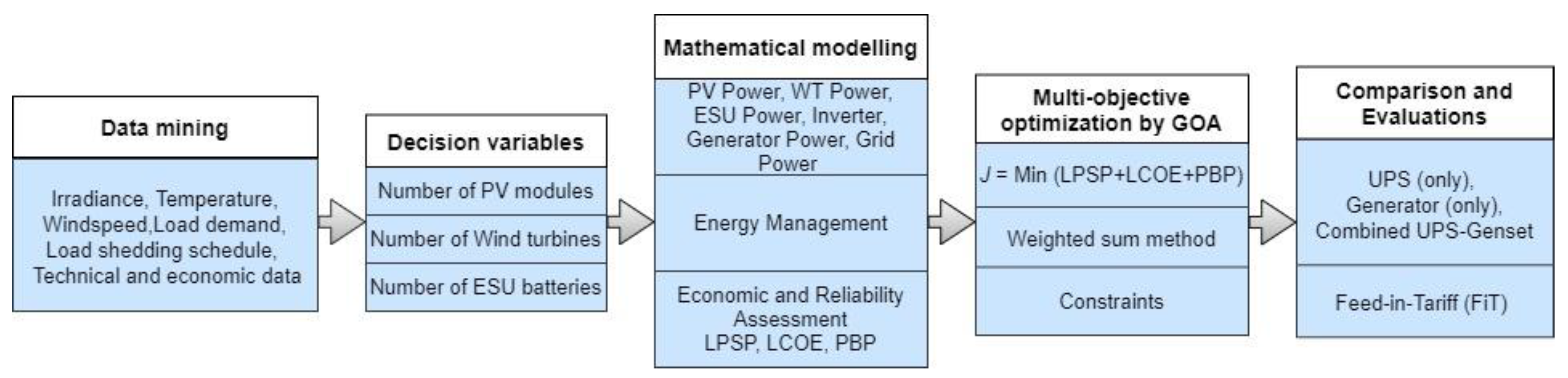
  • The study provides an integrated methodology to determine the best size energy management scheme (EMS) combination for the HRES using the optimisation framework.
  • The optimisation uses the multi-criteria (technical and economic) method to select the most appropriate solution from a set of available options.
  • The weighted sum method protects the consumer and investor’s interests and enables the weighing of the objectives according to their importance.
  • The work presents a detailed assessment of HRES with UPS (only), diesel generator (only), and a combined UPS-generator system.
The remainder of the paper is organised as follows. Section 2 provides the materials and methodology, including the mathematical models of the HRES components, the economic and reliability assessment, the proposed EMS, the formulation of the multi-decision criteria-based optimisation problem, and the description of the considered study area. The results are presented, analysed, and compared in Section 3. Finally, the conclusion is given in Section 4.

2. Materials and Methods

The methodology adopted to accomplish the proposed research is given in Figure 1. The HRES of the PV-WT-ESU-diesel generator system is considered to ensure uninterrupted power supply to a household community suffering scheduled load shedding from the grid. Assumed given are the load shedding schedules, the availability of the endogenous renewable resources, the load demand profile, as well as the relevant technical and economic characteristics of commercially available equipment (rated power, efficiency, and capital cost). The objective is the optimal design of the system that minimises, simultaneously, both the technical and economic objectives. The technical objective considered is the loss of power supply probability (LPSP), which reflects the reliability of the system. The economic objectives are described by two parameters: the levelised cost of electricity (LCOE) and the payback period (PBP), both calculated using life-cycle assessment. The optimisation is performed using a multi-objective GOA using the weighted sum method. Through the use of a weighting factor, which a priori expresses a trade-off between three objectives (LPSP, LCOE, and PBP), a multi-objective optimisation problem is reduced to a single objective and solved in a simplified way. Finally, the performance of the optimised HRES is compared with three conventional methods: diesel generator (only), UPS (only), and a combined generator-UPS system. The simulations are performed on Windows 10 Pro 64-bit Intel (R) Core (TM) i7-2600 CPU @ 3.40 GHz with 8 GB of RAM.

2.1. HRES Architecture and Modelling

The proposed HRES of a multi-bus system is presented in Figure 2. The PV, WT, and ESU are connected to the DC bus, while the generator, grid, and load are directly connected to the AC bus. The PV array is connected by means of a unidirectional DC-DC converter with the maximum power point tracking control. The ESU, constructed from a lead-acid battery bank, is connected via a bidirectional DC-DC converter [24]. To maintain the power balance of the HRES, a central controller with an embedded EMS is used. The controller communicates with the power converters of various sources using control signal paths denoted by the dotted lines.
The energy supply of the system (i.e., the sum of all energy production components) should be equal to the load demand over the entire scheduling time range
( P _ P V ( t ) + P _ W T ( t ) ± P _ E S U ( t ) × η i n v ) + P _ G e n ( t ) ± P _ G r i d ( t ) = P _ L o a d ( t )
Here, P_Load (t) is the load demand at time step (t) and P_PV (t), P_WT (t), P_ESU (t), P_Gen (t) and P_Grid (t) are the power supplied by the PV, WT, ESU, generator, and grid at each t, respectively. The positive/negative sign associated with the ESU and the grid indicates the ability of the sources to generate and absorb the power, respectively. η i n v is the efficiency of the bidirectional inverter. For simplicity, the efficiency of other converters is assumed to be unity.

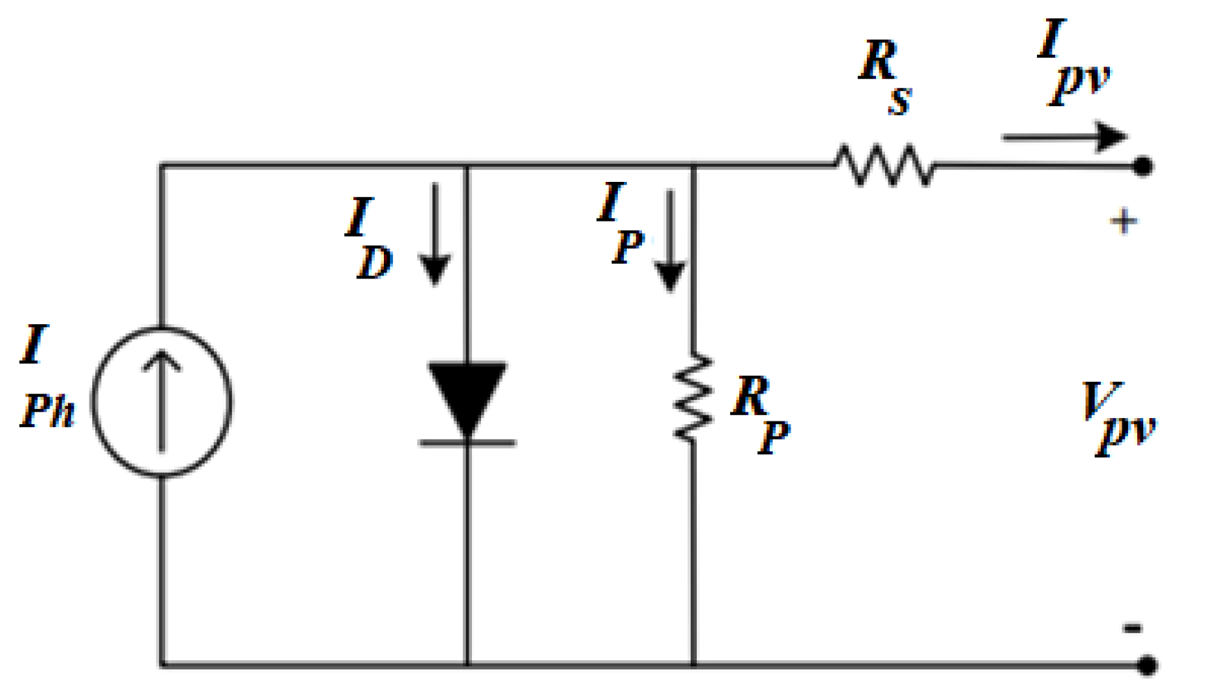
2.1.1. Photovoltaic Model

The power output of PV (P_PV) for any irradiance (G) and temperature (T) can be calculated using a single diode model, as shown in Figure 3 [25]. The output current of PV is given as:
I P V = [ ( I S C S T C + k i ( T T S T C ) ) G G S T C ] I 0 [ ( e ) ( V P V + I P V R S V T ) 1 ] ( V P V + I P V R S R P )
where ISC-STC is the short circuit current at standard test conditions (STC) (i.e., G = 1000 W/m2 and T = 298 K), ki represents the short circuit current coefficient, Io is the leakage current of the diode, VT = akT/q refers to thermal voltage, and a is the ideality factor that ranges between (1 ≤ a ≤ 2) [26]. K represents the Boltzmann constant considered as 1.381 × 10²³ J/K and q is the electron charge considered as 1.602 × 10⁻¹⁹ C. RS and RP are the series and shunt resistances, respectively [27]. For this research, the Kyocera KD325GX-LFB (325 W) solar panel is considered [28]. Different PV parameters used are given in Table A1 in Appendix A. The total output power of the entire array (P_PV) is calculated by multiplying the total number of modules (NPV) with Pmax (t):
P P V ( t ) = N P V × P m a x ( t )

2.1.2. Wind Turbine Model

The power produced by a WT (PWT) at time t can be computed according to [29]:
P W T ( t ) = { 0 v v c u t   i n   or   v v c u t   o f f P r a t e d (   v ( t ) v c u t   i n   v ( t ) v c u t   i n ) 3 v c u t   i n     v < v r a t e d P r a t e d v r a t e d     v < v c u t   o f f
where v, vrated, vcut in, and vcut off are the wind speed, rated speed, cut-in speed, and cut-off speed of the WT, respectively. The total power generated by the installed wind turbines P_WT can be computed as:
P _ W T ( t ) = N W T × P W T ( t )
NWT represents the total number of WT generators. To normalise the wind speed v (measured by an anemometer at a reference height H0) to the desired hub height (H) of the WT under study, the following equation is used [30]:
v = v 0 [ H     H 0   ] α
where v is (m/s) measured at H (m) and v0 is the wind speed calculated at the reference height H0 (m). The constant α is the ground surface friction coefficient; its value lies between 0.1 and 0.25 [31]. The typical value of 1/7 is considered for this study; this value corresponds to low-roughness surfaces and well-exposed sites [30]. Important parameters of the utilised WT EOcycle EO10 (5 kW) are provided in Table A1 in Appendix A.

2.1.3. Energy Storage Model

The ESU is used to complement the energy excess or deficit via the charging or discharging process, respectively. It stores surplus power that is not absorbed by the load and delivers the stored energy when there is a shortfall in the generation. The charging and discharging process of the ESU is controlled by estimating the state-of-charge (SOC) of batteries. The model presented in [32] is used to calculate the SOC of the ESU:
  S O C ( t )   = S O C ( t 1 ) × ( 1 σ ) + ( P B a t ( t ) ) × η B a t
In Equation (7), σ represents the hourly self-discharge rate, which is 0.007% for 1 h [33]. For simplicity, σ is assumed to be zero (ideal battery). η B a t indicates the battery charging and discharging efficiency. It is assumed to be 100% for both cases [34]. P B a t represents the charging and discharging power of battery according to its required and available power, respectively. For longevity, the SOC is bounded by the upper and lower limits (i.e., S O C U ,   S O C L ). The power required by the ESU (P_ESU_Req) is the minimum amount of power that if applied continuously increases the SOC of the ESU from the initial to the upper limit (i.e., SOCU) in the time step Δt. The P_ESU_Req is given as:
P _ E S U _ R e q ( t )   = ( S O C U S O C ( t ) ) × C b a t × N b a t   Δ t
Likewise, the power available for the ESU (P_ESU) is the maximum amount of power that the ESU can deliver continuously before reaching the lower limit (i.e., S O C L ) in one time step. The P_ESU is given as:
P _ E S U ( t )   = ( S O C ( t ) S O C L ) × C b a t × N b a t   Δ t
In Equation (9), N b a t represents the total number of batteries in the ESU while C b a t (in kWh) is the nominal capacity for a single battery. The details of the technical specifications of the considered ESU are given in Table A1 in Appendix A. Initially, the ESU is considered to be 30% charged while the S O C U and S O C L are set as 90% and 10%, respectively [35]. The EMS is designed such that the ESU discharges its energy (when demanded) until the S O C L level is reached. On the other hand, the ESU will be charged until the S O C U limit. However, the power exchange between the grid and the ESU does not only depend on the availability of surplus power and the level of the SOC. It is also influenced by the TOU tariff for grid electricity. For this work, ESU charging from the grid is considered during off-peak hours only.

2.1.4. Generator Model

The main function of a diesel generator is as the secondary backup power source [36], in case the primary backup (i.e., the ESU) is not able to support the load. In this work, a split two-generator system is proposed, as shown in Figure 4. The reason for using two generators is to allow the commitment of suitable generators to closely match the specific load demand. This is to avoid low operating efficiencies, thus minimising fuel consumption. Furthermore, this structure increases the reliability and redundancy of the system. The first generator, Gen1, is smaller (rated at 10 kW) than the second generator, Gen2 (20 kW). The sizes are chosen such that the simultaneous operation of both generators can satisfy the peak load of the intended system. However, the generators are turned on only if there is a need to cover the energy deficit during shedding intervals (i.e., when the PV, WT, and ESU are not able to satisfy the load requirement). The power produced by each generator can be described as:
P G e n ( t ) = P n × η G e n
where P n is the rated power in (kW) provided by the manufacturer and η G e n refers to the efficiency of the generator. As two generators are considered, the total output power of the generators will be P G e n ( t )   = P _ G e n 1 ( t ) + P _ G e n 2 ( t ) . The values of the required generator specifications are given in Table A1 in Appendix A.

2.1.5. Inverter Model

The inverter that ties the AC and DC sources of the HRES is modelled according to its efficiency ( η i n v ) . The ratings for the inverter chosen are based on accommodating the maximum peak load according to [37]:
P i n v = P P e a k η i n v
  P P e a k   is the peak load demand from the system and η i n v shows the efficiency of the inverter. The specifications of the inverter considered are given in Table A1 in Appendix A.

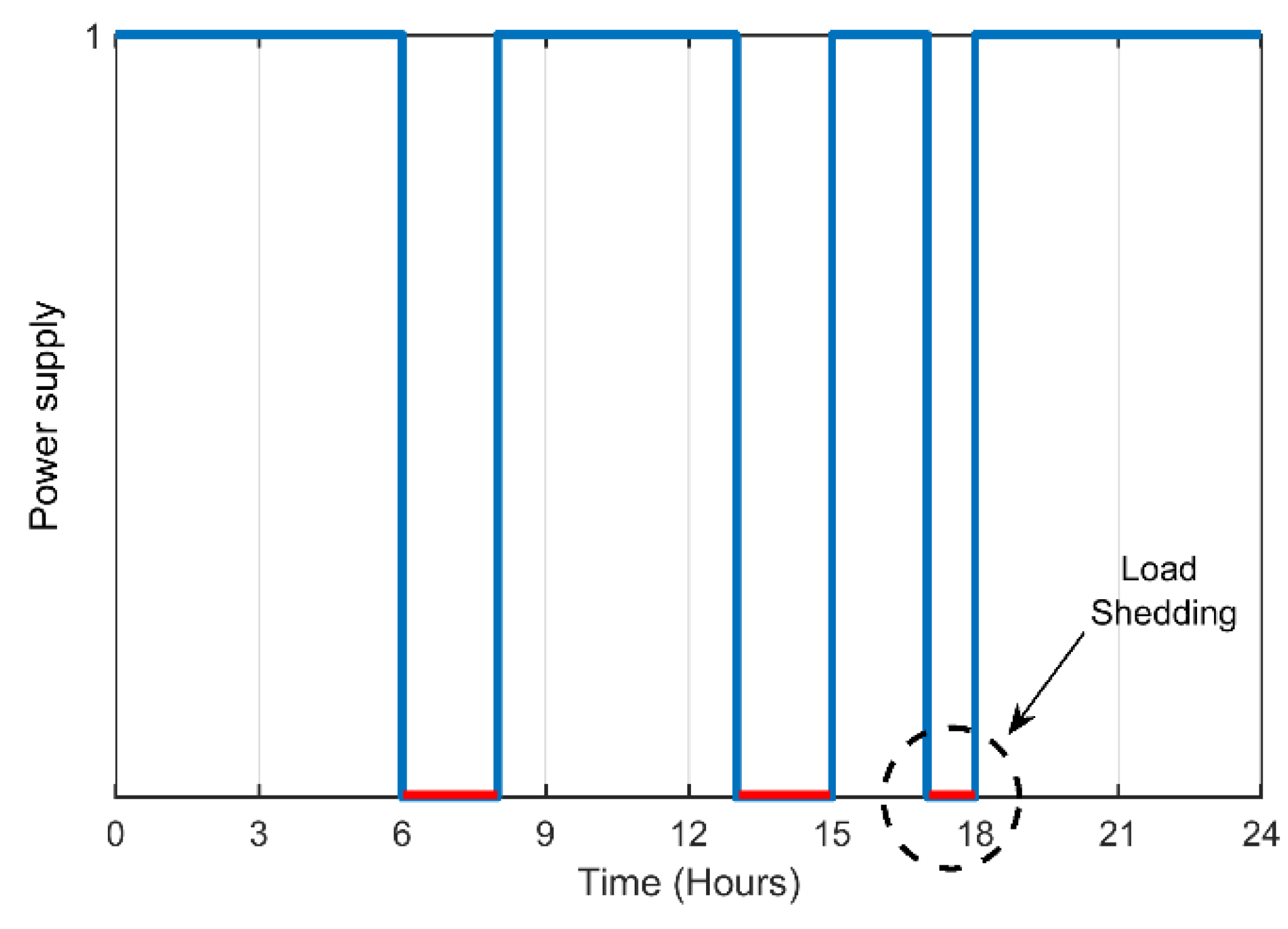
2.1.6. Grid Model with Load Shedding

The grid is intended to satisfy the load demand [36]. Thus, its output power can be expressed as:
P G r i d ( t ) = R G r i d ( t ) × P L o a d ( t )
where RGrid is the reserve capacity margin to ensure the system operates securely when something unexpected happens on the grid. The value of RGrid is assumed to be 1.2, considering the tight constraints and weak conditions of the grid. In this study, the grid is suffering from scheduled load shedding; hence, the Grid-ON and Grid-OFF periods are specified from the power distribution company and are known to the user. This behaviour is considered as the binary state power supply and modelled according to [7,38]:
P G r i d ( t ) = B G r i d ( t ) × P G r i d ( t )
where BGrid (t) is a binary variable that describes the state of the grid at a specific hour. When BGrid (t) = 1, the grid power is available and when BGrid (t) = 0, the grid power is unavailable. Note that grid power can supply the load sufficiently whenever BGrid (t) = 1, Figure 5 demonstrates the status of the grid power supply with periodic load shedding intervals. The off state (depicted on the x-axis) reflects shedding durations. For this typical day, 5 h of load shedding can be observed.

2.2. Economic Assessment

The economic assessment of the HRES is based on two well-known indicators, namely LCOE and PBP [39]. The LCOE determines the cost of electricity but does not consider the revenue opportunities. On the other hand, the PBP considers both the cost and revenue of the system. These indicators are crucial for comprehensive life-cycle analysis and economic feasibility evaluation of the project [40]. The LCOE is more related to consumers while the PBP is attributed to investors. The LCOE is defined as the total cost of the system over its warranted lifetime divided by the total energy production across the same period.
L C O E = T o t a l   S y s t e m   C o s t   T o t a l   E n e r g y   P r o d u c t i o n = n = 1 N C o s t S y s t e m / ( 1 + r ) n E n e r g y S y s t e m / ( 1 + r ) n ( $ k W h )
Here, N represents the project lifetime while r is the discount rate. The system costs (Costsystem) include the initial cost, the operating cost (insurance, running, repairs), and the replacement cost over the project lifetime. All the relevant costs of the HRES are provided in Table A1 in Appendix A. Accordingly, the total energy of the HRES (EnergySystem) is:
E n e r g y H R E S = E n e r g y P V + E n e r g y W T + E n e r g y G e n
The PBP is defined as the period (in years) in which a project reaches its break-even point. Usually, a project with a shorter PBP is more appealing to investors. In its simplest form, the PBP is determined as [41]:
P B P = C o s t s S y s t e m A n n u a l I n c o m e
In Equation (16), the AnnualIncome represents the (yearly) amount of revenue generated by selling HRES energy to the grid under FiT policy.

2.3. Reliability Assessment

The reliability analysis of the HRES is based on the LPSP. It is defined as the probability of power system failure to meet the required load demand:
L P S P = t = 1 T L P S ( t ) t = 1 T P _ L o a d ( t )
  L P S = ( P _ L o a d ( t ) ( P _ P V ( t ) + P _ W T ( t ) + P _ E S U ( t ) × η i n v ) + P _ G e n ( t ) )
where T represents the complete time horizon while t shows the current time step. The value of LPSP ranges between 0 and 1. Zero LPSP means that the load demand is fully satisfied; on the other hand, if the LPSP is unity, the demand is not satisfied at all.

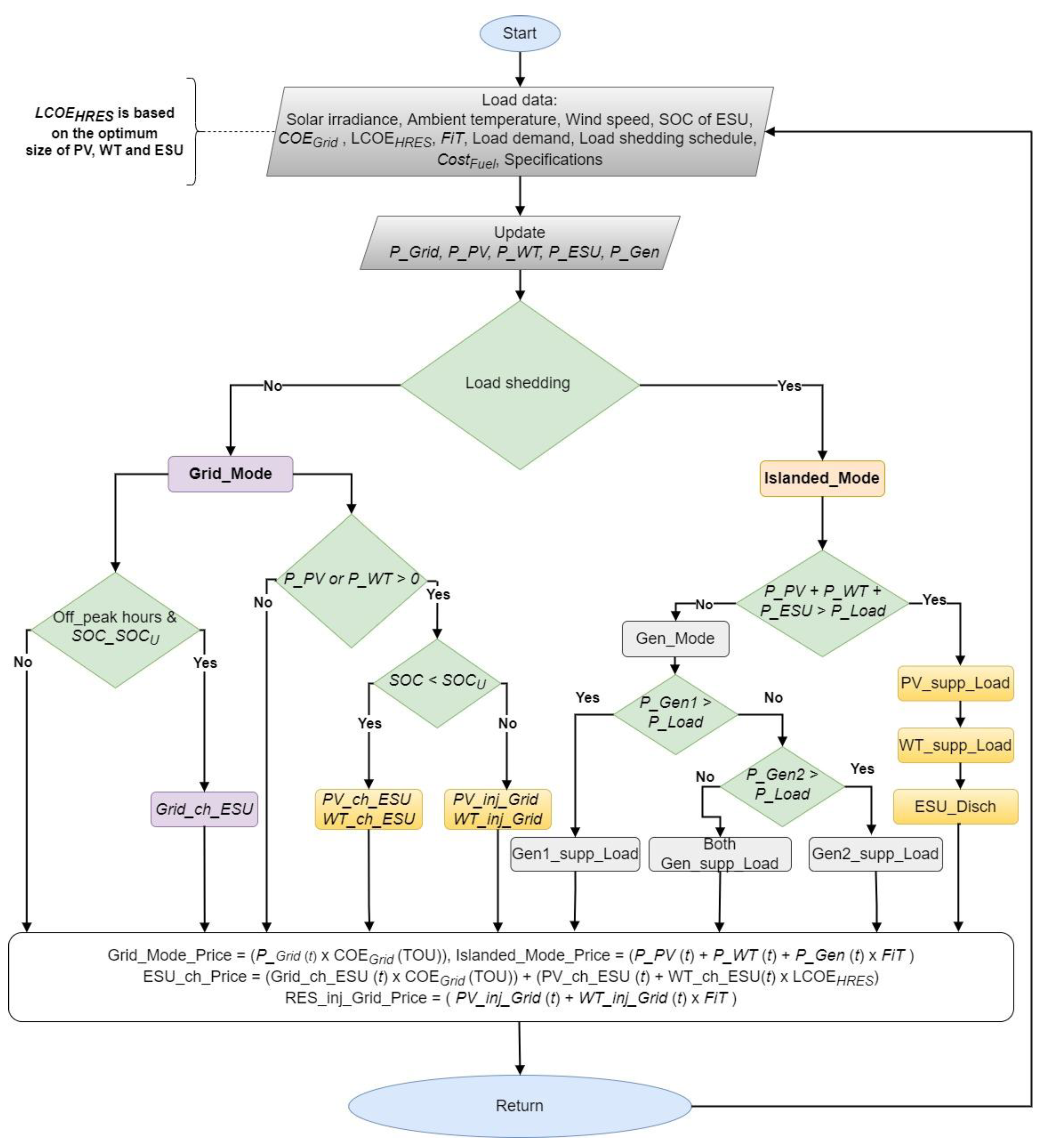
2.4. Energy Management Scheme

The role of energy management becomes inevitable when a system consists of more than one energy source [42]. The main objective of the proposed EMS is to ensure an uninterrupted supply of electricity during load shedding irrespective of the weather and load shedding conditions. The priority is given to PV and WT utilisation to serve the load and charge the ESU. However, if the PV and WT are not sufficiently producing electricity to satisfy the load, the ESU is discharged. The generators are triggered as a last resort if the PV, WT, and ESU cannot meet the load requirement. To perform the aforementioned tasks, the EMS decides on two modes of operation for the HRES. The modes are specified according to the power supply available from the grid.
  • Grid mode: When the grid is supplying power. During this mode, the grid is assumed to have sufficient power to satisfy the load. The surplus of the grid (if available) charges the ESU. For this research, the TOU tariff policy is considered. Thus, ESU charging from the grid takes place during off-peak hours only. Meanwhile, if the PV and WT produce power during this mode, the ESU starts charging. ESU charging from renewables during the availability of grid power provides maximum economic benefits.
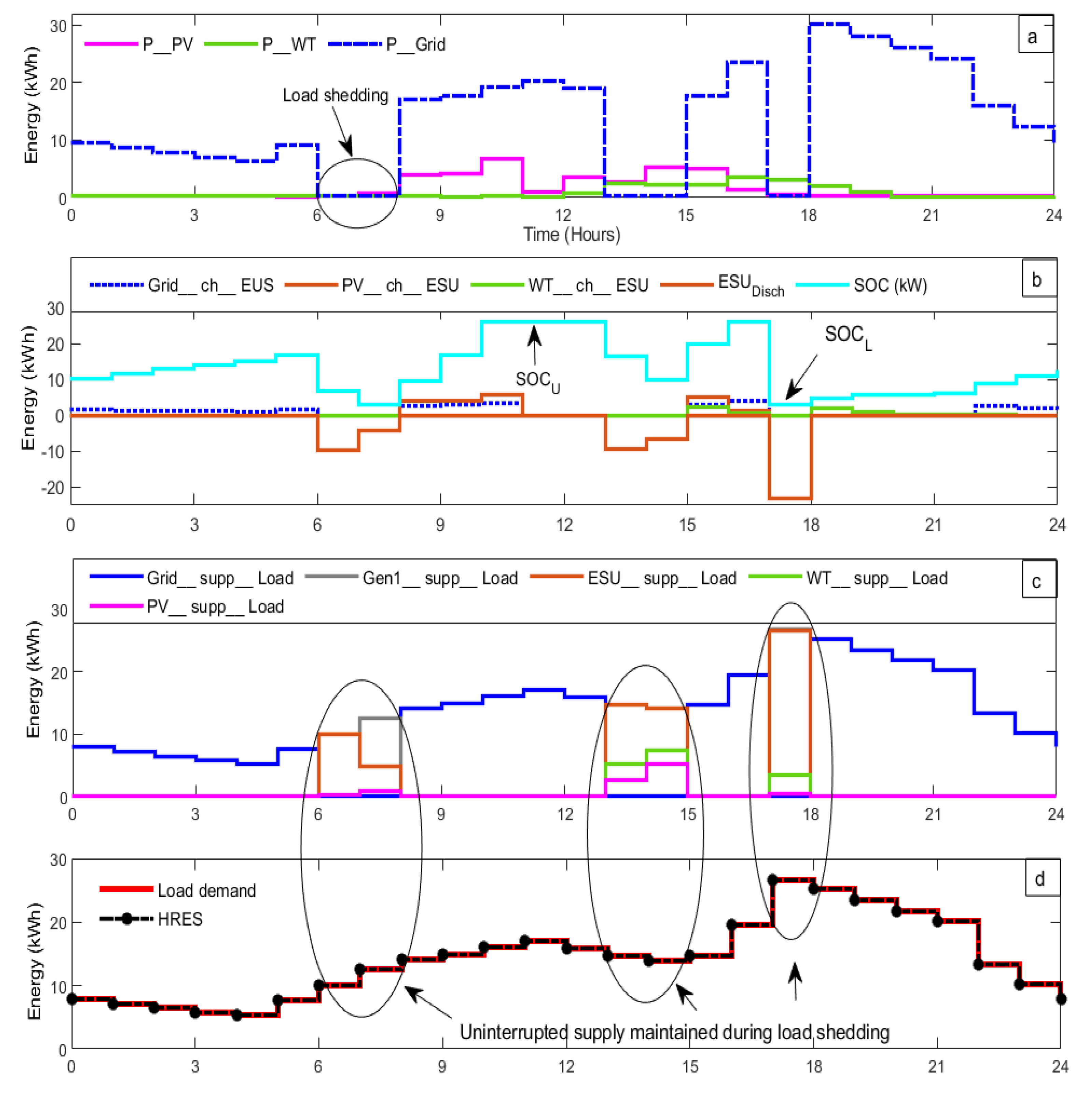
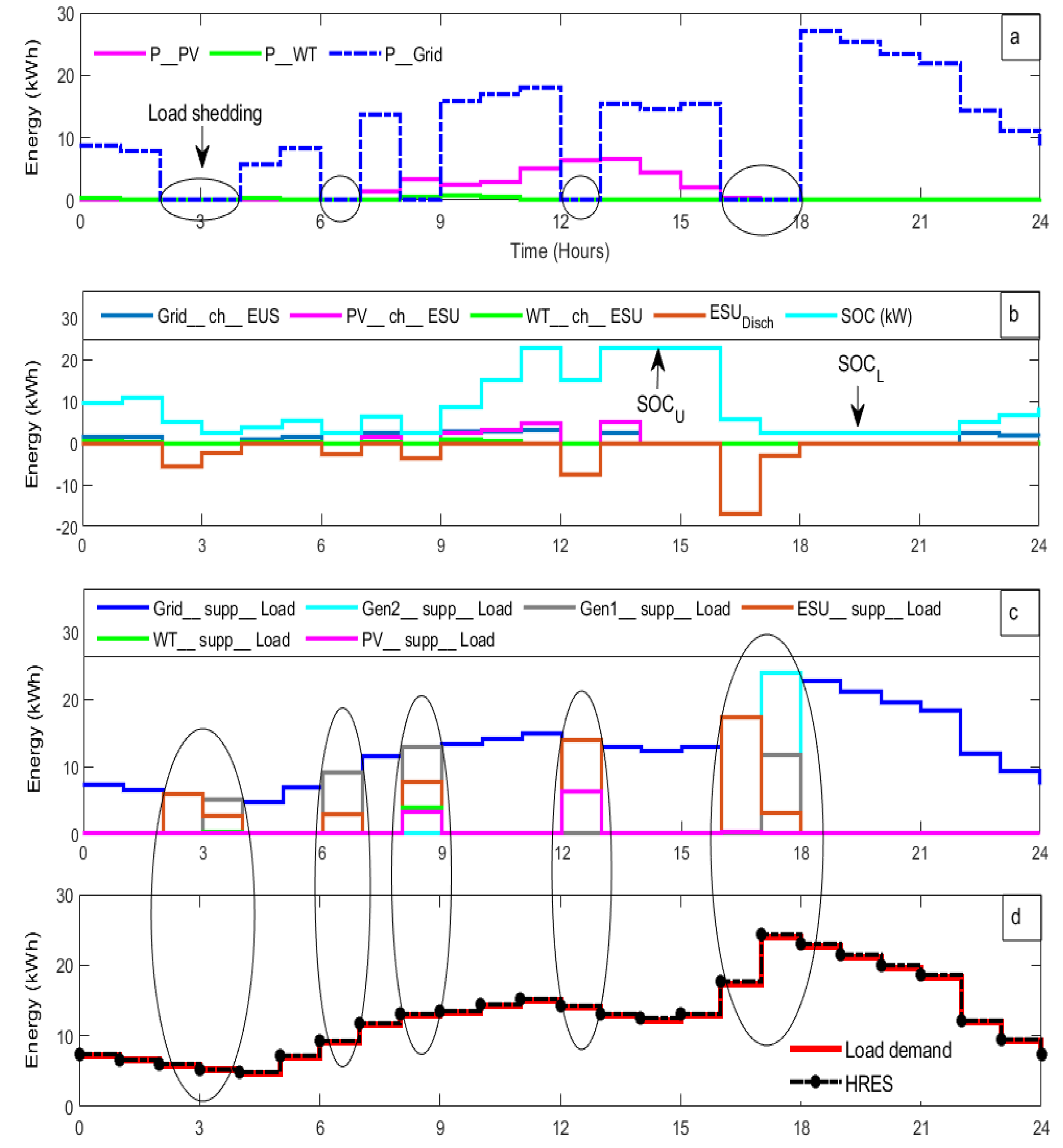
  • Islanded mode: When the power from the utility grid is not available (load shedding duration). The HRES assets are utilised to meet the load requirement. Priority is given to PV and WT power. However, due to the intermittent and weather-dependent nature of these sources and the load variations, the ESU and generators can contribute to power supply operation. The EMS is developed using a rule-based algorithm and is shown in Figure 6.

2.5. Formulation of Objective Function

The process of selecting the most appropriate configuration of the HRES is based on a set of criteria. For this purpose, technical and economic objectives (i.e., LPSP, LCOE, and PBP) are included in the objective function of the HRES. To solve such a multi-criteria problem, there are different approaches suggested in the literature. Among them, the weighted sum method is a popular approach due to its simplicity [43,44]. This method allows the multi-objective optimisation problem to be cast as a single-objective mathematical optimisation problem. The latter is constructed as a sum of objective functions multiplied by weighting coefficients (wi). The main objective function of HRES as a minimisation problem is given as follows:
m i n     J ( n p ) = t m i n ( w 1 × L P S P + w 2 × L C O E + w 3 × P B P )
In Equation (19), w1, w2, and w3 are the weighting coefficients associated with each criterion. The weight value selection depends on the design criterion; the only restriction is that the sum of them must be equal to one [45]. The variable np is the sizing vector: np = {NPV, NWT, NBat}, where NPV and NWT are the number of PV and WT units, respectively. Moreover, NBat is the number of batteries in the ESU. The goal is to find the optimised combination of PV modules, WT units, and ESU batteries that can provide the lowest value of the objective function (LPSP, LCOE, and PBP). However, there are several limits and restrictions to be considered during the optimisation to avoid undesired results. Thus, the objective function is subjected to the following constraints.

2.5.1. Capacity Limit Constraint

The first constraint imposed is the boundaries for the decision variables [46]:
n p = integer ,     n p min   n p     n p max
where np ∈ {NPV, NWT, Nbat} and its value should lie between the maximum and minimum limits. The boundaries are set on the hit-and-trial method in all optimisation algorithms [47]. For this research, the upper and lower limits of the variables are given in Equation (21). The bounds are used to reduce the convergence time.
Variable   range   { 10 < N P V     110 2 < N W T     15 5 < N B a t     20

2.5.2. Battery Charging Constraint

The SOC is set to avoid the overcharging and undercharging of the ESU. This is to minimise the ESU degradation and ageing process [48]. The SOC should be confined within the upper (SOCU) and lower (SOCL) limits, as defined by Equation (22). Moreover, the ESU charges from the renewables when there is surplus power (i.e., during all times). However, its charging from the grid takes place during off-peak hours only. These constraints are formulated via Equations (23)–(25).
S O C L     S O C ( t )     S O C U
  P V _ c h _ E S U ( t ) = P P V ( t ) P L o a d ( t )   for   all   t
  W T _ c h _ E S U ( t ) = P W T ( t ) P L o a d ( t )   for   all   t
G r i d _ c h _ E S U ( t ) = P G r i d ( t ) P L o a d ( t )   for   t = o f f _ p e a k _ h o u r s

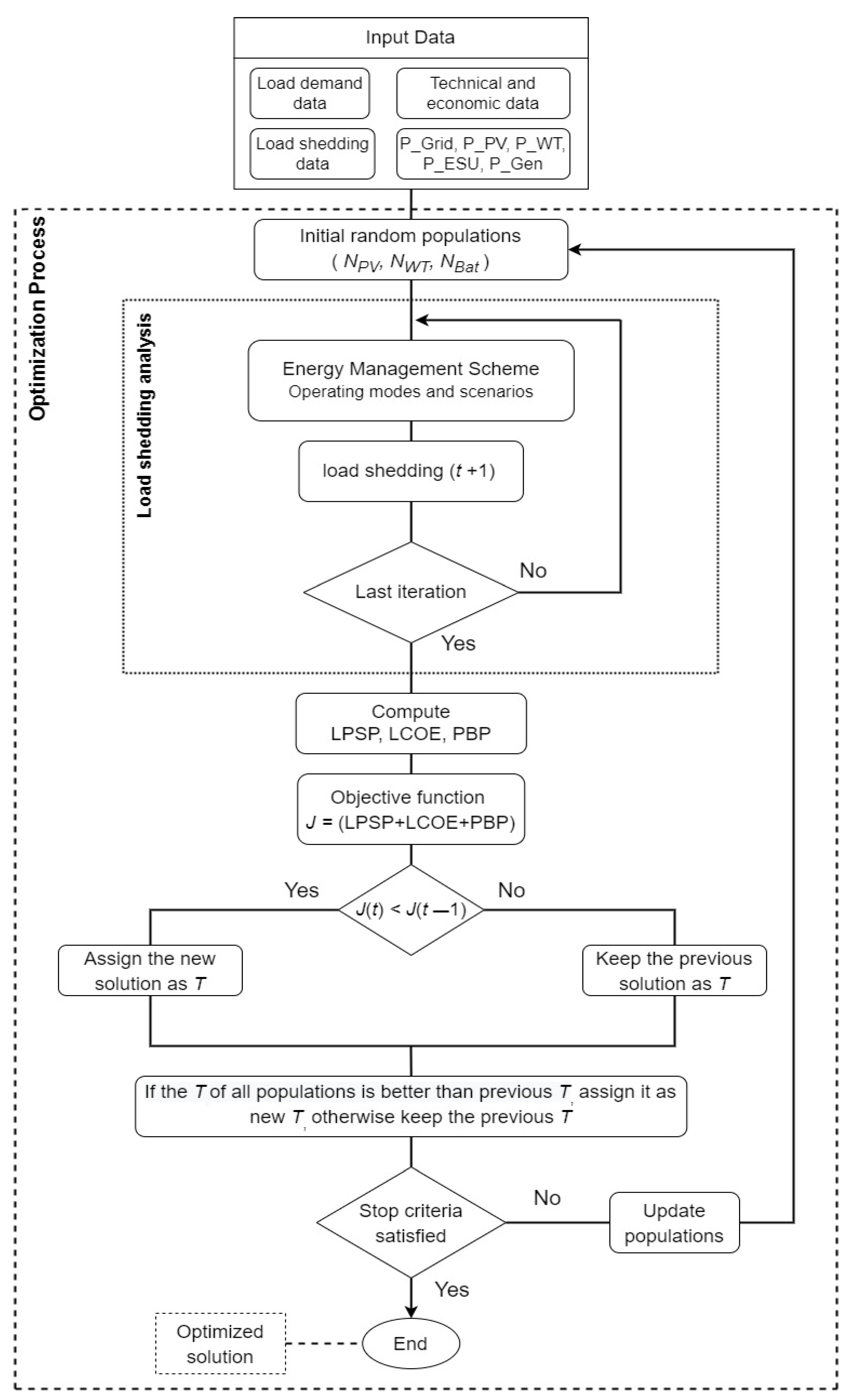
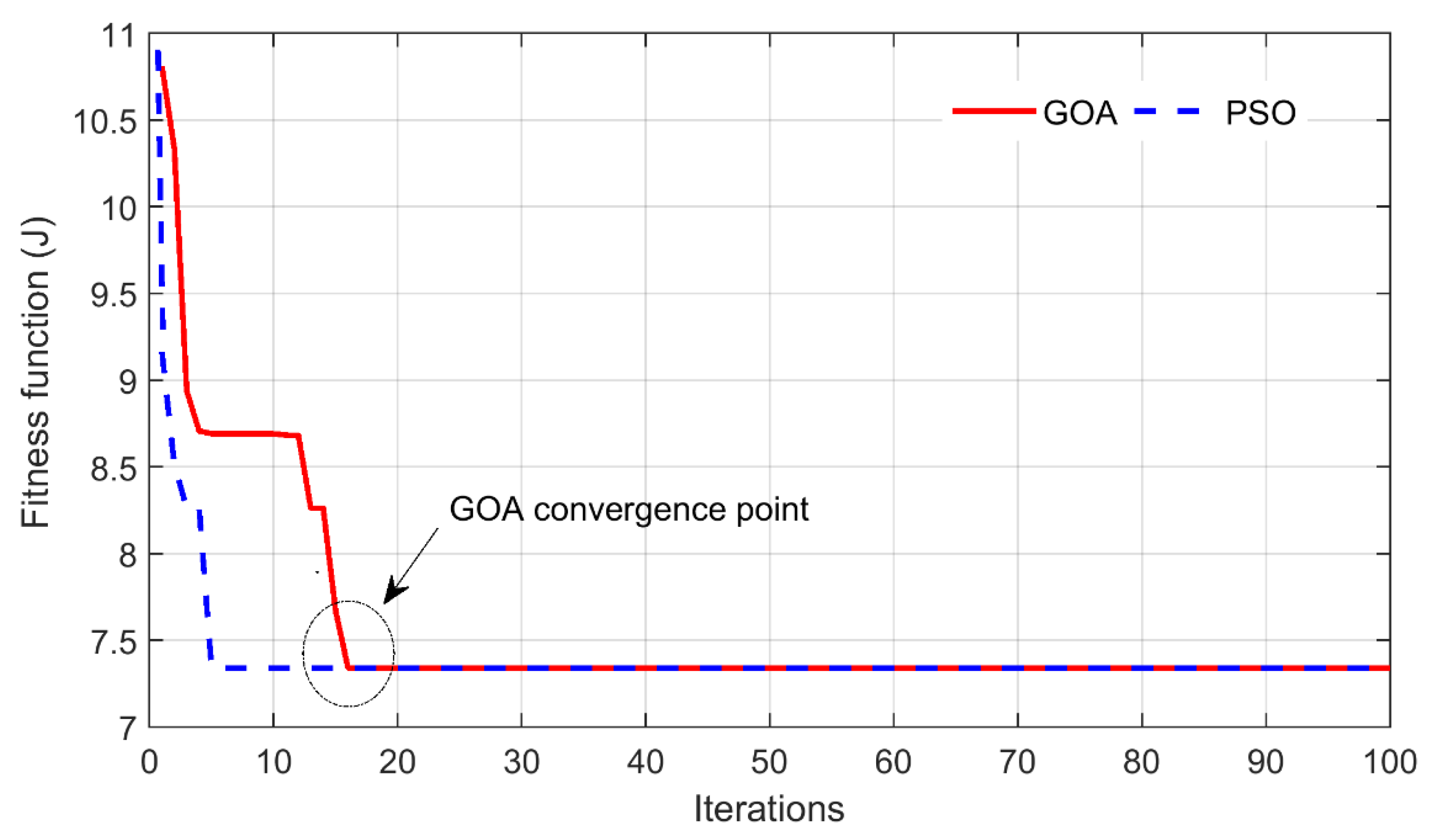
2.5.3. Grasshopper Optimisation Algorithm for Optimal Sizing of HRES Components
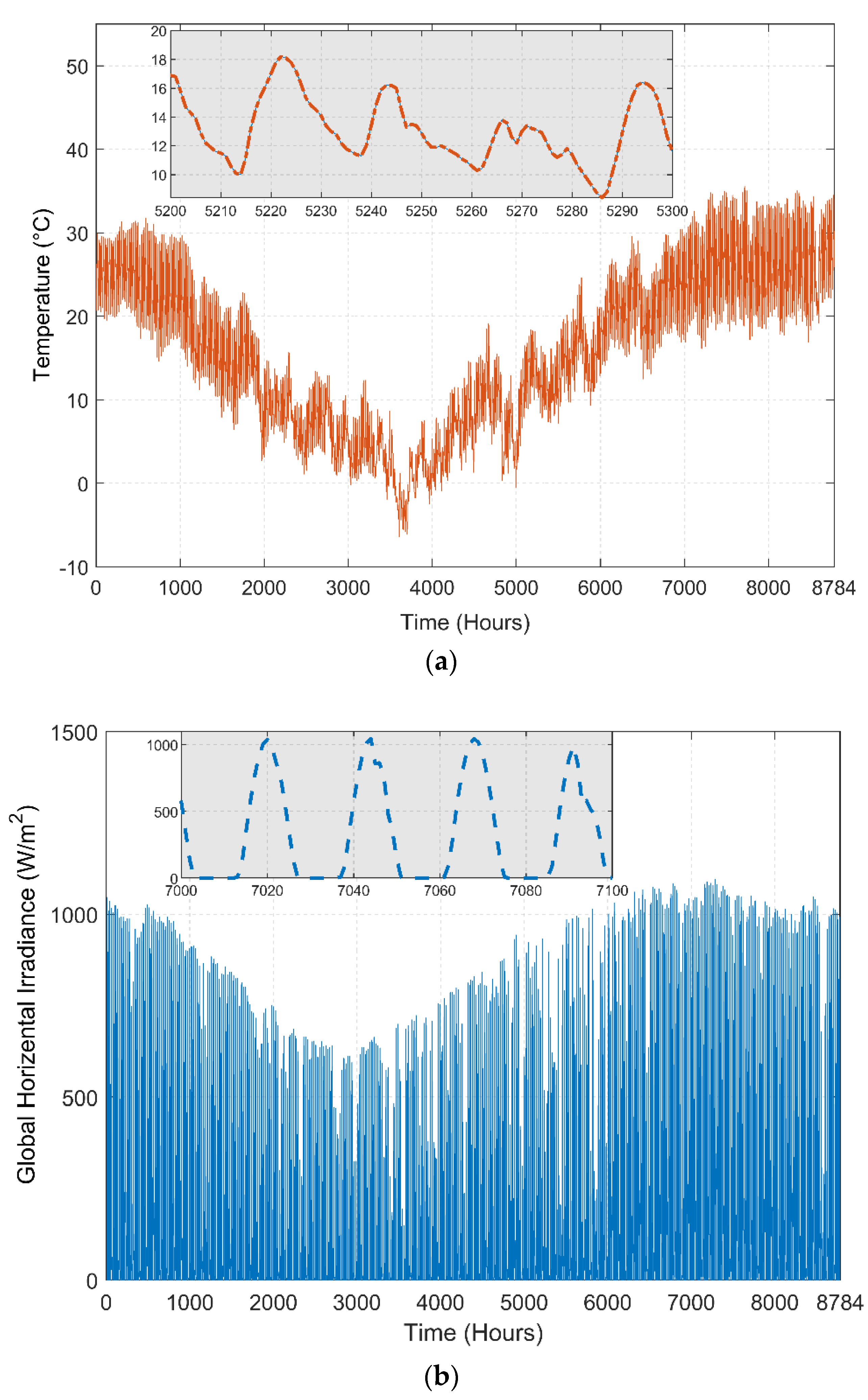
The GOA is a nature-inspired metaheuristic optimisation algorithm proposed by [49]. The algorithm mimics the social conduct of a swarm of grasshoppers when they search for food in nature. The swarm behaviour of grasshoppers is mathematically expressed as follows:
X i d ( k + 1 ) = c   [ j = 1 j i N c   u b d   l b d 2   S   ( | X j   ( k ) X i   ( k ) | ) X j   ( k ) X i   ( k ) d i j ] + T ^ d
where xj and xi show the position of jth and ith grasshopper, respectively. In the dth dimension, u b d and l b d represent the upper and lower bounds, respectively, while k is the value of particles for the current time step, and k + 1 refers to the values of particles for the next time step. The targeted value of the dth dimension is represented by T ^ d . It is referred to as the best solution found so far. c is a decreasing coefficient used to shrink the comfort zone, repulsion zone, and attraction zone of the grasshoppers. It is used twice to simulate the deceleration process of the grasshoppers. The first c minimises the search region (towards the targeted grasshopper) when the iteration increases. Accordingly, the second c is used to minimise the effect of attraction and repulsion forces between grasshoppers. The value of the adaptive parameter c is updated using Equation (26). The mechanism improves the balance between exploitation and exploration of the GOA and reduces the comfort zone proportionally with the increasing number of iterations.
c = c m a x k c m a x c m i n K m a x
c m a x and the c m i n are the maximum and the minimum values of c, respectively. K represents the ongoing iteration, while kmax represents the maximum number of iterations. The position of a grasshopper is updated based on its current position, global best position, and the positions of other grasshoppers within the swarm. This helps the GOA to avoid being trapped in local optima. For this work, the GOA is employed to solve the sizing problem. The optimisation framework integrating the GOA (for optimal sizing) and the proposed EMS to address the load shedding problem is shown in Figure 7. At the start of the simulation, the GOA places some random particles from the search landscape whose limits are specified by the user (refer to Equation (21)). These particles move in the search landscape in accordance with the governing equations of the algorithm, thereby optimising the formulated objective function. The optimisation algorithm stops when it reaches the preset stopping criteria.

2.5.4. Study Area

The proposed HRES is tested using a case study of a small residential community situated in Quetta City, a region in Baluchistan, Pakistan. The geographical location is identified with the latitude and longitude of 30.1798° N and 66.9750° E, respectively. Quetta and its surrounding districts have very poor electric power infrastructure; hence, the daily load shedding lasts several hours. On the other hand, Quetta has tremendous potential for indigenous renewables, particularly solar. The annual climatological data (i.e., solar irradiance, ambient temperature, and wind speed) are shown in Figure 8. The hourly data are sourced from Solcast (solar resource assessment and forecasting data), logged from August 2019 to August 2020 [50]. The mean value of daily irradiance is 5518 kWh/m2/day, while the mean ambient temperature (Tamb) is 26 °C. The mean wind speed (v) is 2.28 m/s at an anemometer height of 10 m. The data for G, v, and Tamb are plotted below, showing the hourly values during a year (8784 data).
Quetta is predominantly characterised by two seasons (i.e., summer and winter). The summer begins in April and ends in October with a maximum Tamb of 35.6 °C. Accordingly, the winter commences from November to March with a minimum Tamb of −6.4 °C. The load demand for the considered location (for 40 houses and limited public facilities) is shown in Figure 9 [51]. Two load profiles are considered: one for the summer season and the other for the winter season. Energy consumption during the summer is higher than in the winter due to the excessive use of air conditioning. The daily consumption for the given community is 345 and 309 kWh for summer and winter seasons, respectively. Accordingly, the peak power usage is 26.66 and 23.91 kW, respectively.

3. Results and Discussion

The proposed optimisation framework is implemented in a MATLAB environment. The simulations are performed using the yearly (2019–2020) dataset of solar radiation, wind speed, and ambient temperature of the studied location for the given load profile. The data are sourced from Solcast (solar resource assessment and forecasting data), which provides genuine hourly average processed historical data [50]. The hourly resolution is favourable for the optimisation as its accuracy is widely accepted for yearly energy performance calculations, while it facilitates a faster computation time than higher resolution datasets. The load shedding schedules are derived from [52].
To perform the simulation, first the optimal sizes of HRES components (NPV, NWT, NESU) are determined using the GOA and benchmarked to the particle swarm optimisation algorithm (PSO). The GOA is the more recent metaheuristic algorithm; it has been successfully applied in several sizing problems, for example [53,54]. On the other hand, PSO is an older algorithm that has been extensively used in diverse applications [55]. The application of PSO to the HRES is the same as the GOA (referred to Figure 7). Note that the source code of the GOA and PSO can be found in [56]. The choice of the selection of the controlling parameters for the GOA and PSO are given in Table 2.
The optimization is achieved by minimizing the value of the fitness function given in Equation (19). As the fitness function is a multi-objective function that constitutes three variables, namely LPSP, LCOE, and PBP, each objective function is assigned an equal weightage of 0.33 to avoid the influence of any objective. The normalisation is performed as each objective function has different magnitudes than the others [44]. The normalisation process allows the fitness function to have the same magnitude for each contributing element during the computation phase. As the population-based algorithms are stochastically-based, getting a solution using a single run may not be conclusive [57]. To improve the reliability of the results, GOA and PSO algorithms are run separately across 5 individualistic runs with 100 iterations. The trend of fitness function convergence (with respect to iterations) for these two algorithms is given in Figure 10.
Since the optimisation objective is to minimise the multi-objective function, the runs with the lowest values represent the best solution. For the GOA, the red dashed curve in Figure 10a provides the best result. The obtained fitness function value ( J ) for this run is 7.34. In the case of PSO, the blue dashed curve in Figure 10b represents the best result. A comparison of the best curves of both algorithms is given in Figure 11. It was found that both algorithms converge at approximately the same fitness value (J = 7.34) leading to the same number of optimal components for PV, WT, and batteries to be installed. These results validate the accuracy and the reliability of the optimal sizing results. However, the PSO algorithm converges faster than the GOA, i.e., at the 5th iteration.
Table 3 presents the results for the HRES for the best runs. The optimum sizes of NPV, NWT, and NBat are 110, 2, and 16 units, respectively. The computed LCOE is 6.64 cents/kWh, which is a lower value than the grid electricity (9.3 cents/kWh). This suggests that the HRES is a viable solution to the load shedding problem. The value of LPSP is 0.0092, which is also satisfactory over a scale of 0–1. The 0 value of LPSP means that the load will always be satisfied by the given configuration, while 1 indicates that the load will never be satisfied. Accordingly, the PBP of 7.4 years is an attractive proposition, considering the 25-year lifespan of the HRES project.
The HRES is designed based on the specifications of the components given in Table A1 and obtained optimal configuration (i.e., the PV array rated at 35.75 kW, the WT rated at 10 kW, and the ESU rated at 28.8 kWh). In addition, two diesel generators rated 10 and 20 kW are used as the secondary backup.

3.1. Test Scenarios

The performance of the optimised HRES is tested under moderate and harsh conditions. In moderate conditions, normal weather and average load shedding conditions are applied. On the contrary, harsh conditions refer to extreme weather conditions and load shedding schedules. These scenarios are deliberately chosen to observe the resiliency of the HRES. Resiliency here is defined as the ability of the HRES to provide the customers with uninterrupted electricity, regardless of the load shedding patterns and meteorological conditions. The simulations are performed for the load demand shown previously (i.e., in Figure 9). The same HRES configuration (NPV, NWT, NBat) is used for the test scenarios.

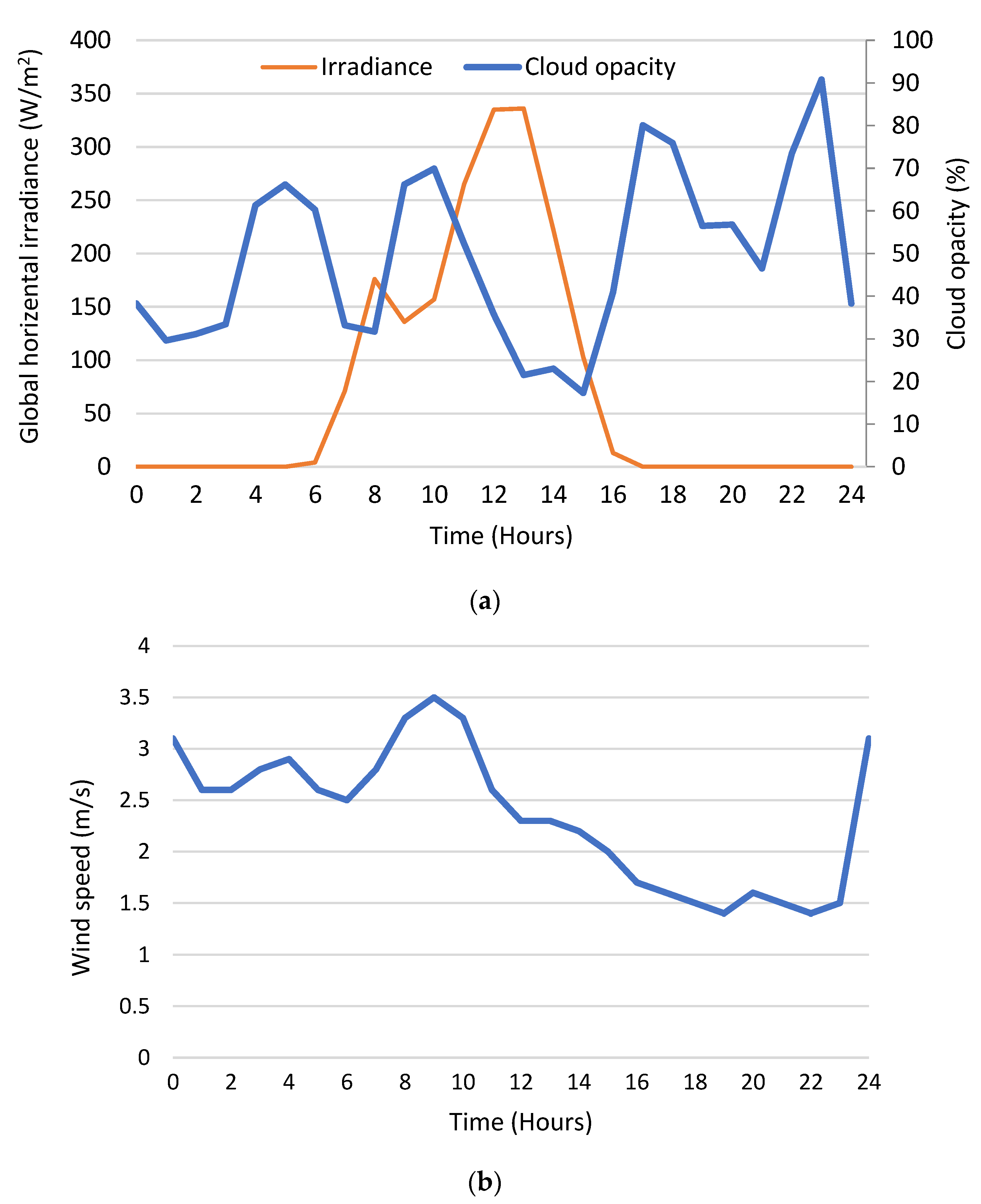
3.1.1. Moderate Conditions

The weather profiles of the considered location on a moderate day are shown in Figure 12. Due to the significant influence of cloudiness on the irradiance, the cloud opacity is plotted to show the weather condition of the considered day in plot (a). The plot shows the conditions of a specific summer day, where during the daytime (i.e., 9:00–15:00), a high incidence of solar radiation is observed. The low cloud opacity indicates clear sky, which defines the moderate weather condition of this day [32]. Accordingly, the wind profile of the given day is shown in plot (b).
The HRES and EMS operations for a sunny summer day are depicted in Figure 13. The results are shown in four plots. Plot (a) shows the status of the available power on the considered day. Different power sources shown are grid supply (P_Grid), PV power (P_PV), and WT power (P_WT). Accordingly, plot (b) shows the charging and discharging of the ESU with the variation of SOC, while plot (c) represents the energy transactions between different sources (i.e., Grid, PV, WT, ESU, Gen1, and Gen2). Finally, plot (d) shows the power delivered by the HRES against the load demand. If the former can track the contour of the latter, it is assumed that resiliency is achieved.
As obvious from the grid supply in plot (a), load shedding is imposed for 5 h, divided into three separate trenches (i.e., hours 6–8, 13–15, and 17–18). In plot (b), it can be noted that the SOC variations are consistent with the charging and discharging trend of the ESU. It is charged under three conditions: (1) from the grid during off-peak hours (shown by the Grid_ch_ESU trace), (2) during the excess of PV power (PV_ch_ESU), and (3) during the excess of WT power (WT_ch_ESU). On the other hand, the ESU discharges (to support the grid) during the load shedding intervals. In plot (b), negative ESUDisch indicates that the battery is discharging. At any hour, the energy delivered by the ESU is given as:
  P E S U ( t ) = P _ L o a d ( t ) / η i n v ( P P V ( t ) + P _ W T ( t ) )
In Equation (28), it is possible that P E S U ( t ) < 0. This situation indicates the surplus PV and WT energy being absorbed by the ESU. However, it must be within the bounds of SOCU and SOCL. The flow of power by different sources is shown in plot (c). The Grid_Mode is active when the grid sufficiently satisfies the load. On the other hand, during the absence of the grid power, the renewable sources (i.e., PV, WT, and ESU) supply the required load, thus activating the Islanded_Mode. For this specific day, there is no need to turn on the generator because these sources are sufficient to support the grid. During the Islanded_Mode, the EMS ensures that PV utilisation is given the highest priority, as can be clearly observed during hours 6–8 and 13–15. Furthermore, as the irradiance is high, PV alone can satisfy the load; other sources are not utilised. At hours 17–18, the load shedding reoccurs during the peak hour, where demand is the highest. As PV is not producing sufficient power, WT and ESU also support the grid during this period. The ability of the HRES to satisfy the fluctuating load demand can be seen in plot (d). Clearly, the system is resilient throughout the day, without the need to utilise any of the generators.

3.1.2. Harsh Conditions

Under harsh conditions, the weather profile of a selected day is shown in Figure 14. The intensity of irradiation on this day is much lower than in summer (refer to plot (a)). In addition, the influence of daytime cloud cover on the irradiance can be observed, thus indicating the harsh weather conditions of this day. Likewise, the wind speed of the given day is also very low (no more than 3.5 m/s), as shown in Figure 13b. The same HRES configuration (NPV, NWT, NBat) is used while the load demand for the winter season is used.
The HRES performance for the extreme winter day is illustrated in Figure 15. The load shedding happens for 7 h, divided into five separate trenches (refer to plot (a)). The first trench happens at night for two consecutive hours (i.e., hours 2–4). As there is no irradiance and PV power during nighttime, the ESU supports the grid for the first hour (plot (b)). However, during the second hour (3–4), Gen1 has to support as the ESU cannot sustain the required load. Notice that Gen1 is operated because the power deficit (less than 10 kW) is lower than the capacity of the smaller generator. During the second trench of shedding at hours 6–7, again, the demand is fulfilled by Gen1 and the ESU because PV production has not started. In the third trench of load shedding at hours 8–9, the PV, WT, and ESU start supplying. However, as the demand increases, the generator has to be utilised. The duration of the generator in operation is determined by the present SOC (refer to plot (b)). If SOCL is reached, Gen1 is turned on. At noon (i.e., hours 12–13), the PV and ESU coordinate together to supply the load. Accordingly, load shedding is imposed again at hours 16–18. The ESU discharges and satisfies the load during the first hour (16–17). However, it reaches its maximum allowed limit to discharge. As the load demand is higher than the capacity of Gen1 due to the peak hours, the EMS activates Gen2 to support the load. During this day, both Gen1 and Gen2 have to operate because of the extreme winter conditions. The energy transactions of different sources are demonstrated in plot (c). Accordingly, the HRES operation with variable load can be observed in plot (d). Despite the limited PV and WT yield, the HRES satisfies the load demand through integrated operation of all the energy sources in the system.

3.1.3. Comparison with Conventional Solutions

The feasibility of the HRES is compared to the conventional load shedding mitigation methods, namely, diesel generator (only), UPS (only), and a combined system (generator-UPS). For the generator (only) solution, Gen1 and Gen2 with the same specifications used for the HRES are considered. Furthermore, the same diesel price (69 cents/L) is considered. For the solution that utilises UPS only, NBat = 19, while for the combined UPS-generator, NBat = 10. For both cases, NBat is determined using the GOA. These sizes are based on the minimum value of the LCOE and PBP while fulfilling the load requirement (i.e., LPSP = 0). The simulations are performed using the same meteorological data and load shedding schedules.
The performance of all mitigation methods based on the one-year data is presented in Table 4. For the HRES, the annual working hours for the generators are only 190 h. On the other hand, for the solution using generators (only), the generators have to be turned on for 1678 h. Meanwhile, if a generator is combined with a UPS, the time to turn on is reduced to 1160 h. From the results, it is clear that the inclusion of renewable sources in the HRES significantly reduces the fuel consumption of generators.
Furthermore, as cost is the main consideration for HRES installation, a detailed comparison of the economic aspects is required. Thus, the LCOE and PBP for the conventional solutions are calculated according to Equations (14) and (16). As with the HRES, calculations for conventional systems are based on the 25-year system lifetime. Accordingly, the annual income for the PBP calculation is based on the FiT and LCOE for the HRES and conventional sources, respectively, which can be calculated as:
AnnualIncome_HRES = Total Energy Contribution × FiT
AnnualIncome_Conventional System = Total Energy Contribution × LCOESource
The results of the comparison are shown in Table 5. It can be observed that, although the HRES has a high capital cost, it exhibits the lowest LCOE (6.64 cents/kWh) and PBP (7.4 years). The PBP suggests that the system will pay for itself after 7.4 years. On the other hand, the conventional generator (only) solution has the lowest capital. However, due to the high diesel consumption over the lifespan of the project, its LCOE is approximately four times higher than the HRES (i.e., 29.68 cents/kWh). The LCOE of the UPS (only) solution is 13.23 cents/kWh. The cost is mainly due to the periodical replacement of the batteries. In addition, the higher grid electricity price for charging also contributes to the operational cost. Finally, for the combined system (generator-UPS), the LCOE is 19.82 cents/kWh. The PBP for these conventional systems is 9.8 years for UPS, 12.9 years for diesel generators, and 11.3 years for the combined system (UPS-generator).
In addition to the benefit of having the lowest LCOE and PBP, the HRES also reduces the grid burden by injecting surplus renewable power from the PV and WT into the grid. The annual contribution from the renewables is 32,361 kWh, which translates to a load reduction of 47.2%, 32.9%, and 42.3% compared to the UPS (only), generator (only), and combined UPS-generator case, respectively.
The results clearly prove the cost-effectiveness of the HRES over conventional methods to mitigate the load shedding problem. Furthermore, the PBP estimation shows that the HRES investment is economically attractive and also offers a high profit margin for investors.

3.1.4. Comparison with Similar Studies

The LCOE of the HRES obtained in the current study has been compared with other studies addressing the grid intermittency problem. The optimal configurations from different locations tabulated in Table 6 show a variation in LCOE. The most vocal factors in LCOE variation are the localised meteorological conditions, fuel and equipment costs, capacity shortage, and subsidies on renewable installations. In addition, the time of the power requirement (day vs night) from the alternate hybrid system also directly affects the LCOE. A comparison of the proposed HRES with existing studies shows better or very competitive results. Referring to Table 6, the proposed HRES provides an optimal solution in terms of lower LCOE. Therefore, it is concluded that the presented GOA-based optimisation (implemented in MATLAB) is more cost-effective compared to HOMER to mitigate the load shedding problem.

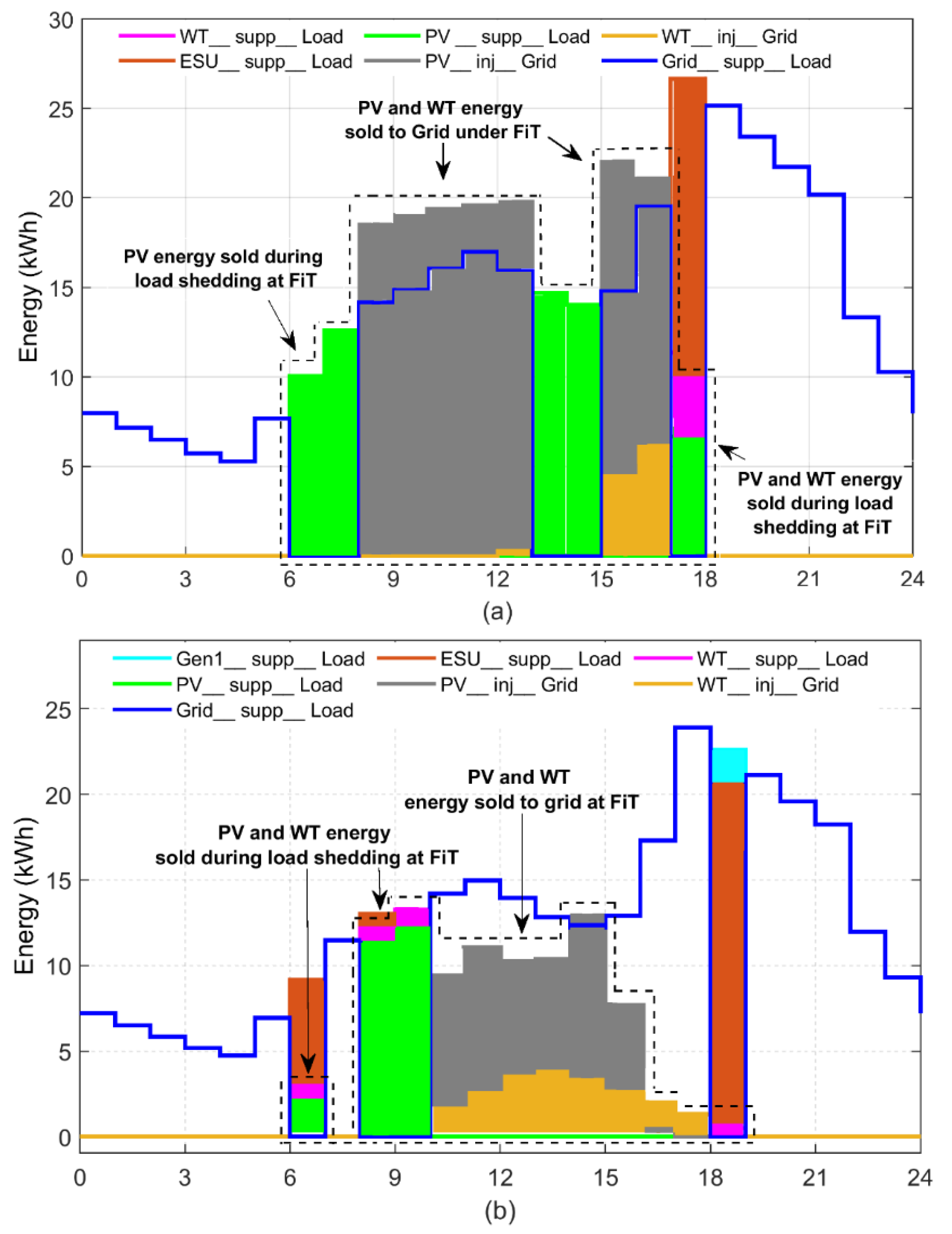
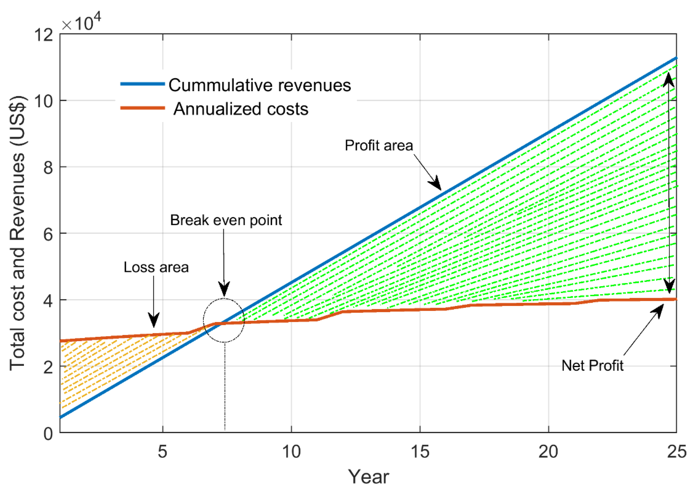
3.1.5. Feed-in Tariff and Payback Period Evaluation for the HRES

Recall that the PBP is based on the total project costs and the annual income of the system. The latter depends on the amount of the yearly contribution from the renewable sources of the HRES. This contribution comes from the direct supply of renewable energy served during load shedding and the surplus energy injected into the grid, at the agreed FiT plan. Note that the FiT is the special selling price allocated to renewable energy generators for injecting renewable energy into the grid. For Pakistan, the levelised FiT structure for one unit of electricity over 25 years and the COEGrid are provided in Table 7 [58]. The FiT scheme is not very attractive due to the high cost of grid electricity; in fact, during peak time, the FiT is lower than the COEGrid.
To illustrate the impact of the FiT on the PBP, HRES operation during typical summer and winter day scenarios is used. The contribution of renewables is shown in Figure 16. As expected, due to higher irradiance on a summer day, the PV injects more energy into the grid. Note that the FiT takes place when the renewable energy is utilised during the load shedding intervals and when the extra energy is injected into the grid. The contribution of PV and WT is shown by filled pink and green areas during load shedding intervals, respectively, while their injection into the grid is highlighted with filled grey and yellow areas. The PV and/or WT injection into the grid occurs when they have surplus power during Grid_mode.
The PBP analysis is assisted by Figure 17, which represents the annualised costs and the revenue flow of the HRES. The linearity of the revenue curve is due to the assumption that load demand is constant throughout the project life cycle. On the other hand, the non-linearity of the annualised cost curve is because of the discounted and replacement costs of HRES components. This replacement (battery, inverter) must be made at different intervals during the project lifespan. The cumulative annualised costs integrate the capital costs and the adjusted O&M costs according to the incurred time. Notice that for the HRES operational period (25 years), the total annualised costs are equivalent to the total costs of the optimal configuration of the HRES (USD 39,884). The profit-loss break-even point is at 7.4 years. Beyond this PBP, the project starts earning. For the remaining project lifetime, the net profit amounts to approximately USD 75,000.
The PBP assessment shows that the HRES investment is economically attractive and also offers a high profit margin for investors. These results can help policymakers in the affected countries to promote renewable policies and encourage private investment.

4. Conclusions

This work has optimised HRES—a combination of renewable sources, storage elements, and generators—to overcome the load shedding problem. Given the technical specifications of components, meteorological, and demand data with load shedding schedules, the methodology can determine the number of PV panels, wind turbines, and battery units along with generator hours to achieve the minimum LCOE and PBP of the system while ensuring power supply availability. The case study is presented for a small residential community (with actual load shedding conditions) situated in Quetta, Pakistan. The results show that the optimally designed HRES has the potential to effectively mitigate the problem of load shedding compared to the conventional solutions. The LCOE of the HRES is 6.64 cents/kWh, which is below the LCOE of the diesel generator (only) (29.68 cents/kWh), UPS (13.23 cents/kWh), and the combined generator-UPS system (19.82 cents/kWh). Furthermore, the HRES alleviates the grid burden by 47.2%, 32.9%, and 42.3%, respectively. The break-even analysis has shown that the PBP of the HRES is 7.4 years. This shows that HRES investment is economically attractive and also offers a high return opportunity for investors. The estimated profit of the system is USD 75,000 over the 25-year project lifespan. The main conclusion from this work is that an optimised HRES can be utilised to alleviate the energy crisis faced by several developing nations. This solution can be integrated into the existing infrastructure and is aligned with the Sustainable Development Goal (SDG-7) of the United Nations that ensures “reliable, affordable, sustainable, and modern energy for all”.
The present research can be improved by considering the environmental criteria (such as CO2 reduction) along with technical and economic criteria in the future.

Author Contributions

Conceptualisation, M.P.B. and Z.S.; methodology, M.P.B. and Z.S.; formal analysis, M.P.B. and Z.S.; investigation, M.P.B., Z.S., M.A.K. and A.L.B.; funding acquisition, W.A., M.G., M.A.K. and N.K.; resources, Z.S.; software, M.P.B. and N.K.; supervision, Z.S. and M.G.; validation, Z.S., M.G. and W.A.; visualisation, N.K., M.G. and A.L.B.; writing—review and editing, M.P.B., Z.S. and M.G. All authors have read and agreed to the published version of the manuscript.

Funding

Authors received no funding for this research.

Data Availability Statement

The data that support the findings of this study were derived from the openly available data in a public repository at https://solcast.com/ (accessed: 18 August 2020) and http://ccms.pitc.com.pk/FeederDetails (accessed: 15 June 2020) by providing required information.

Acknowledgments

This article has been made possible with the support of the Centre of Electrical Energy Systems (CEES), School of Electrical Engineering, Universiti Teknologi Malaysia (UTM), and the Higher Education Commission, Pakistan.

Conflicts of Interest

The authors declare no conflict of interest.

Nomenclatures

α On-off binary variable
Δ t Time step (hour)
η B a t Battery efficiency (%)
η G e n Generator efficiency (%)
η I n v Inverter efficiency (%)
C b a t Nominal battery capacity (kWh)
COEGridGrid cost of electricity ($/kWh)
CostFuelFuel cost (($/L)
ESU_DischEnergy discharge from ESU (kWh)
Gen1_supp_LoadGenerator 1 energy being supplied to load (kWh)
Gen2_supp_LoadGenerator 2 energy being supplied to load (kWh)
Grid_ch_ESUGrid energy charging ESU (kWh)
Grid_supp_LoadGrid energy being supplied to load (kWh)
hTime step (hour)
N B a t Number of batteries
N P V Number of PV units
N W T Number of wind turbines
P_ESUESU output power (kW)
P_ESU_ReqPower required by ESU to reach SOCU (kW)
P_GenDiesel generator output power (kW)
P_Gen1Generator 1 output power (kW)
P_Gen2Generator 2 output power (kW)
P_GridGrid power (kW)
P_HRESOutput power of HRES
P_LoadEnergy demand (kW)
P_PVPV output power (kW)
P r a t e d Generator rated power (kW)
PV_ch_ESUPV energy charging ESU (kWh)
PV_inj_GridPV energy being injected to grid (kWh)
PV_supp_LoadPV energy being supplied to load
P_WTWT output power (kW)
P m a x PV maximum output power
wiWeight for objective function i
WT_ch_ESUWT energy charging ESU (kWh)
WT_inj_GridWT energy being injected to grid (kWh)
WT_supp_LoadWT energy being supplied to load
SOCCState of charge of ESU current hour (kWh)
SOCUUpper limit of state of charge (kWh)
SOCLLower limit of state of charge (kWh)
Abbreviations
EMSEnergy management scheme
ESUEnergy storage unit
FiTFeed in tariff
GOAGrasshopper optimization algorithm
HRESHybrid renewable energy system
LCOELevelised cost of electricity
LPSPLoss of power supply probability
PBPPayback period
PSOParticle swarm optimization
PVPhotovoltaic
TOUTime of use
WTWind turbine

Appendix A

Table A1. Technical and economic specifications of HRES components.
ComponentParameterVariableValuesUnits
PVRated power (per module)
Module efficiency
Performance ratio
Initial (capital) cost [59]
Operating cost (yearly) [59]
Expected lifetime
PPV
r
PR
ICPV
OCPV
LifePV
325
17.0
0.75
305
3.05
25
W
%
-
$/kW
$/kW
Years
WTRated power
Start-up wind speed
Survival wind speed
Rated wind speed
Rotor diameter
Blades
Initial (capital) cost [60]
Operating cost (yearly) [60]
Expected lifetime
PWT
vcut in
vcut off
vrated
-
-
ICWT
OCWT
LifeWT
5
3
50
10
5.4
3
600
6.0
25
kW
m/s
m/s
m/s
m
-
$/kW
$/kW
Years
ESURated capacity
Charging/discharging efficiency
Initial (capital) cost
Replacement cost (After 5 years)
Expected lifetime
CBat
η B a t
ICBat
RCBat
LifeBat
1800
100
250
250
5
Wh
%
$/kWh
$/kWh
Years
GenRated power
Generator efficiency
Power factor
Initial (capital) cost
Operating cost (yearly) [60]
Fuel cost
Expected lifetime
PGen
η G e n
PF
ICGen
OCGen
FCGen
LifeGen
10 + 20
90.0
0.8
180
0.064
0.690
15,000
kW
%
-
$/kW
$/Hour
$/Liter
Hours
InverterRated power
Inverter efficiency
Initial (capital) cost
Replacement cost (After 10 years)
Expected lifetime
Pinv
η i n v
ICInv
RCInv
LifeInv
30
95
1669
1669
10
kW
%
$
$
Years
Other economic parametersProject lifetime [61]
Discount rate [61]
PV degradation rate [61]
WT degradation rate [62]
Fuel curve intercept coefficient [53]
Fuel curve slope [53]
N
r
DEGPV
DEGWT
C1
C2
25
5
0.50
0.60
0.246
0.0814
Years
%
%
%
L/kWh
L/kWh
Balance of system costWiring, dc cable, ac main panel, EMS controller, charge controller, MPPT, breaker box and converterBOS1000$

References

  1. Hossain, S.M.; Hasan, M.M. Energy management through bio-gas based electricity generation system during load shedding in rural areas. Telkomnika Telecommun. Comput. Electron. Control 2018, 16, 525–532. [Google Scholar]
  2. Anjum, Z.M.; Said, D.M.; Hassan, M.Y.; Leghari, Z.H.; Sahar, G. Parallel operated hybrid Arithmetic-Salp swarm optimizer for optimal allocation of multiple distributed generation units in distribution networks. PLoS ONE 2022, 17, e0264958. [Google Scholar] [CrossRef]
  3. Mbomvu, L.; Hlongwane, I.T.; Nxazonke, N.P.; Qayi, Z.; Bruwer, J.-P. Load Shedding and its Influence on South African Small, Medium and Micro Enterprise Profitability, Liquidity, Efficiency and Solvency. Bus. Re-Solut. Work. Pap. BRS/2021/001 2021. [Google Scholar] [CrossRef]
  4. Bevrani, H.; Tikdari, A.G.; Hiyama, T. Power system load shedding: Key issues and new perspectives. World Acad. Sci. Eng. Technol. 2010, 65, 199–204. [Google Scholar]
  5. Shrestha, R.S. Electricity Crisis (Load Shedding) in Nepal, Its Manifestations and Ramifications. Hydro Nepal J. Water Energy Environ. 2010, 6, 7–17. [Google Scholar] [CrossRef]
  6. Shi, B.; Liu, J. Decentralized control and fair load-shedding compensations to prevent cascading failures in a smart grid. Int. J. Electr. Power Energy Syst. 2015, 67, 582–590. [Google Scholar] [CrossRef] [Green Version]
  7. Siraj, K.; Awais, M.; Khan, H.A.; Zafar, A.; Hussain, A.; Zaffar, N.A.; Jaffery, S.H.I. Optimal power dispatch in solar-assisted uninterruptible power supply systems. Int. Trans. Electr. Energy Syst. 2019, 30, e12157. [Google Scholar] [CrossRef]
  8. Ani, V.A. Design of a Reliable Hybrid (PV/Diesel) Power System with Energy Storage in Batteries for Remote Residential Home. J. Energy 2016, 2016, 6278138. [Google Scholar] [CrossRef] [Green Version]
  9. Malik, P.; Awasthi, M.; Sinha, S. A techno-economic investigation of grid integrated hybrid renewable energy systems. Sustain. Energy Technol. Assess. 2022, 51, 101976. [Google Scholar] [CrossRef]
  10. Wu, T.; Zhang, H.; Shang, L. Optimal sizing of a grid-connected hybrid renewable energy systems considering hydroelectric storage. Energy Sources Part A Recover. Util. Environ. Eff. 2020, 1–17. [Google Scholar] [CrossRef]
  11. Ahuja, D.; Tatsutani, M. Sustainable energy for developing countries. SAPI EN. S. Surv. Perspect. Integr. Environ. Soc. 2009, 2, 2009. [Google Scholar]
  12. Altbawi, S.M.A.; Mokhtar, A.S.B.; Arfeen, Z.A. Enhacement of microgrid technologies using various algorithms. Turk. J. Comput. Math. Educ. 2021, 12, 1127–1170. [Google Scholar]
  13. Sinha, S.; Chandel, S. Review of recent trends in optimization techniques for solar photovoltaic–wind based hybrid energy systems. Renew. Sustain. Energy Rev. 2015, 50, 755–769. [Google Scholar] [CrossRef]
  14. Anjum, W.; Husain, A.R.; Aziz, J.A.; Rehman, S.M.F.U.; Bakht, M.P.; Alqaraghuli, H. A Robust Dynamic Control Strategy for Standalone PV System under Variable Load and Environmental Conditions. Sustainability 2022, 14, 4601. [Google Scholar] [CrossRef]
  15. Almutairi, K.; Dehshiri, S.H.; Dehshiri, S.H.; Mostafaeipour, A.; Issakhov, A.; Techato, K. Use of a Hybrid Wind—Solar—Diesel—Battery Energy System to Power Buildings in Remote Areas: A Case Study. Sustainability 2021, 13, 8764. [Google Scholar] [CrossRef]
  16. Ayub, S.; Ayob, S.; Tan, C.W.; Ayub, L.; Bukar, A.L. Optimal residence energy management with time and device-based preferences using an enhanced binary grey wolf optimization algorithm. Sustain. Energy Technol. Assess. 2020, 41, 100798. [Google Scholar] [CrossRef]
  17. Falama, R.Z.; Welaji, F.N.; Dadjé, A.; Dumbrava, V.; Djongyang, N.; Salah, C.; Doka, S. A Solution to the Problem of Electrical Load Shedding Using Hybrid PV/Battery/Grid-Connected System: The Case of Households’ Energy Supply of the Northern Part of Cameroon. Energies 2021, 14, 2836. [Google Scholar] [CrossRef]
  18. Rehman, S.U.; Rehman, S.; Shoaib, M.; Siddiqui, I.A. Feasibility study of a grid-tied photovoltaic system for household in Pakistan: Considering an unreliable electric grid. Environ. Prog. Sustain. Energy 2019, 38, e13031. [Google Scholar] [CrossRef]
  19. Ndwali, P.K.; Njiri, J.G.; Wanjiru, E.M. Optimal Operation Control of Microgrid Connected Photovoltaic-Diesel Generator Backup System Under Time of Use Tariff. J. Control. Autom. Electr. Syst. 2020, 31, 1001–1014. [Google Scholar] [CrossRef]
  20. Amrr, S.M.; Alam, M.S.; Asghar, M.S.J.; Ahmad, F. Low cost residential microgrid system based home to grid (H2G) back up power management. Sustain. Cities Soc. 2018, 36, 204–214. [Google Scholar] [CrossRef]
  21. Bakht, M.P.; Salam, Z.; Bhatti, A.R.; Sheikh, U.U.; Khan, N.; Anjum, W. Techno-economic modelling of hybrid energy system to overcome the load shedding problem: A case study of Pakistan. PLoS ONE 2022, 17, e0266660. [Google Scholar] [CrossRef] [PubMed]
  22. Bakht, M.; Salam, Z.; Bhatti, A.; Anjum, W.; Khalid, S.; Khan, N. Stateflow-Based Energy Management Strategy for Hybrid Energy System to Mitigate Load Shedding. Appl. Sci. 2021, 11, 4601. [Google Scholar] [CrossRef]
  23. Samy, M.; Mosaad, M.I.; Barakat, S. Optimal economic study of hybrid PV-wind-fuel cell system integrated to unreliable electric utility using hybrid search optimization technique. Int. J. Hydrog. Energy 2020, 46, 11217–11231. [Google Scholar] [CrossRef]
  24. Liu, N.; Zou, F.; Wang, L.; Wang, C.; Chen, Z.; Chen, Q. Online energy management of PV-assisted charging station under time-of-use pricing. Electr. Power Syst. Res. 2016, 137, 76–85. [Google Scholar] [CrossRef]
  25. Chin, V.J.; Salam, Z.; Ishaque, K. Cell modelling and model parameters estimation techniques for photovoltaic simulator application: A review. Appl. Energy 2015, 154, 500–519. [Google Scholar] [CrossRef]
  26. Ishaque, K.; Salam, Z. An improved modeling method to determine the model parameters of photovoltaic (PV) modules using differential evolution (DE). Sol. Energy 2011, 85, 2349–2359. [Google Scholar] [CrossRef]
  27. Ishaque, K.; Salam, Z.; Taheri, H. Accurate MATLAB Simulink PV System Simulator Based on a Two-Diode Model. J. Power Electron. 2011, 11, 179–187. [Google Scholar] [CrossRef] [Green Version]
  28. Kyocera, “KD325GX-LFB,” Kyocera Solar. Available online: https://www.kyocerasolar.com/ (accessed on 1 June 2019).
  29. Xu, X.; Hu, W.; Cao, D.; Huang, Q.; Chen, C.; Chen, Z. Optimized sizing of a standalone PV-wind-hydropower station with pumped-storage installation hybrid energy system. Renew. Energy 2019, 147, 1418–1431. [Google Scholar] [CrossRef]
  30. Ilinca, A.; McCarthy, E.; Chaumel, J.-L.; Rétiveau, J.-L. Wind potential assessment of Quebec Province. Renew. Energy 2003, 28, 1881–1897. [Google Scholar] [CrossRef]
  31. Mohseni, S.; Brent, A. Economic viability assessment of sustainable hydrogen production, storage, and utilisation technologies integrated into on- and off-grid micro-grids: A performance comparison of different meta-heuristics. Int. J. Hydrog. Energy 2020, 45, 34412–34436. [Google Scholar] [CrossRef]
  32. Bhatti, A.R.; Salam, Z.; Sultana, B.; Rasheed, N.; Awan, A.B.; Sultana, U.; Younas, M. Optimized sizing of photovoltaic grid-connected electric vehicle charging system using particle swarm optimization. Int. J. Energy Res. 2018, 43, 500–522. [Google Scholar] [CrossRef] [Green Version]
  33. Zhang, L.; Barakat, G.; Yassine, A. Design and optimal sizing of hybrid PV/wind/diesel system with battery storage by using DIRECT search algorithm. In Proceedings of the 15th International Power Electronics and Motion Control Conference (EPE/PEMC) EPE-PEMC 2012 ECCE Europe, Novi Sad, Serbia, 4–6 September 2012; pp. 1–7. [Google Scholar]
  34. Vrettos, E.I.; Papathanassiou, S.A. Operating policy and optimal sizing of a high penetration RES-BESS system for small isolated grids. IEEE Trans. Energy Convers. 2011, 26, 744–756. [Google Scholar] [CrossRef]
  35. Altbawi, S.M.A.; Mokhtar, A.S.B.; Jumani, T.A.; Khan, I.; Hamadneh, N.N.; Khan, A. Optimal Design of Fractional Order PID Controller based Automatic Voltage Regulator System Using Gradient-Based Optimization Algorithm. J. King Saud. Univ. Eng. Sci. 2021. [Google Scholar] [CrossRef]
  36. Kebede, A.A.; Berecibar, M.; Coosemans, T.; Messagie, M.; Jemal, T.; Behabtu, H.A.; Van Mierlo, J. A Techno-Economic Optimization and Performance Assessment of a 10 kWP Photovoltaic Grid-Connected System. Sustainability 2020, 12, 7648. [Google Scholar] [CrossRef]
  37. Bukar, A.L.; Tan, C.W.; Yiew, L.K.; Ayop, R.; Tan, W.S. A rule-based energy management scheme for long-term optimal capacity planning of grid-independent microgrid optimized by multi-objective grasshopper optimization algorithm. Energy Convers. Manag. 2020, 221, 113161. [Google Scholar] [CrossRef]
  38. Alramlawi, M.; Gabash, A.; Mohagheghi, E.; Li, P. Optimal operation of hybrid PV-battery system considering grid scheduled blackouts and battery lifetime. Sol. Energy 2018, 161, 125–137. [Google Scholar] [CrossRef]
  39. Sigarchian, S.G. Small-Scale Decentralized Energy Systems: Optimization and Performance Analysis. Ph.D. Thesis, School of Industrial Engineering and Management, KTH Royal Institute of Technology, Stockholm, Sweden, 2018. [Google Scholar]
  40. Zhang, Y.; Ma, T.; Campana, P.E.; Yamaguchi, Y.; Dai, Y. A techno-economic sizing method for grid-connected household photovoltaic battery systems. Appl. Energy 2020, 269, 115106. [Google Scholar] [CrossRef]
  41. Ma, T.; Javed, M.S. Integrated sizing of hybrid PV-wind-battery system for remote island considering the saturation of each renewable energy resource. Energy Convers. Manag. 2019, 182, 178–190. [Google Scholar] [CrossRef]
  42. Aziz, A.; Tajuddin, M.; Adzman, M.; Ramli, M.; Mekhilef, S. Energy Management and Optimization of a PV/Diesel/Battery Hybrid Energy System Using a Combined Dispatch Strategy. Sustainability 2019, 11, 683. [Google Scholar] [CrossRef] [Green Version]
  43. Borhanazad, H.; Mekhilef, S.; Ganapathy, V.G.; Modiri-Delshad, M.; Mirtaheri, A. Optimization of micro-grid system using MOPSO. Renew. Energy 2014, 71, 295–306. [Google Scholar] [CrossRef]
  44. Grodzevich, O.; Romanko, O. Normalization and Other Topics in Multi-Objective Optimization. Proc. Fields MITACS Ind. Probl. Work. 2006, 2, 89–101. [Google Scholar]
  45. Torres-Madroñero, J.; Nieto-Londoño, C.; Sierra-Pérez, J. Hybrid Energy Systems Sizing for the Colombian Context: A Genetic Algorithm and Particle Swarm Optimization Approach. Energies 2020, 13, 5648. [Google Scholar] [CrossRef]
  46. Hannan, M.A.; Tan, S.Y.; Al-Shetwi, A.Q.; Jern, K.P.; Begum, R.A. Optimized controller for renewable energy sources integration into microgrid: Functions, constraints and suggestions. J. Clean. Prod. 2020, 256, 120419. [Google Scholar] [CrossRef]
  47. Barakat, S.; Ibrahim, H.; Elbaset, A.A. Multi-objective optimization of grid-connected PV-wind hybrid system considering reliability, cost, and environmental aspects. Sustain. Cities Soc. 2020, 60, 102178. [Google Scholar] [CrossRef]
  48. Li, X.; Hui, D.; Lai, X. Battery Energy Storage Station (BESS)-Based Smoothing Control of Photovoltaic (PV) and Wind Power Generation Fluctuations. IEEE Trans. Sustain. Energy 2013, 4, 464–473. [Google Scholar] [CrossRef]
  49. Saremi, S.; Mirjalili, S.; Lewis, A. Grasshopper Optimisation Algorithm: Theory and application. Adv. Eng. Softw. 2017, 105, 30–47. [Google Scholar] [CrossRef] [Green Version]
  50. Engerer, N. Historical and Typical Meteorological Year. Available online: https://solcast.com/historical-and-tmy/ (accessed on 8 August 2020).
  51. Bakht, M.P.; Salam, Z.; Bhatti, A.R. Investigation and modelling of load shedding and its mitigation using hybrid renewable energy system. In Proceedings of the 2018 IEEE 7th International Conference on Power and Energy (PECon), Kuala Lumpur, Malaysia, 3–4 December 2018; pp. 35–40. [Google Scholar]
  52. Ministry of Energy (Power Division), Load Management Portal. Available online: http://ccms.pitc.com.pk/FeederDetails (accessed on 15 June 2020).
  53. Bukar, A.L.; Tan, C.W.; Lau, K.Y. Optimal sizing of an autonomous photovoltaic/wind/battery/diesel generator microgrid using grasshopper optimization algorithm. Sol. Energy 2019, 188, 685–696. [Google Scholar] [CrossRef]
  54. Sultana, U.; Khairuddin, A.B.; Sultana, B.; Rasheed, N.; Qazi, S.H.; Malik, N.R. Placement and sizing of multiple distributed generation and battery swapping stations using grasshopper optimizer algorithm. Energy 2018, 165, 408–421. [Google Scholar] [CrossRef]
  55. Tiwari, S.; Kumar, A. Advances and bibliographic analysis of particle swarm optimization applications in electrical power system: Concepts and variants. Evol. Intell. 2021, 1–25. [Google Scholar] [CrossRef]
  56. Unbreen, A.; Abbas, G.; Zafrullah, M. Optimized Grid Connected Model for Power Generation for A University Campus. Pak. J. Sci. 2019, 71, 50. [Google Scholar]
  57. Abualigah, L.; Diabat, A.; Mirjalili, S.; Elaziz, M.A.; Gandomi, A.H. The Arithmetic Optimization Algorithm. Comput. Methods Appl. Mech. Eng. 2021, 376, 113609. [Google Scholar] [CrossRef]
  58. Zafar, U.; Rashid, T.U.; Khosa, A.A.; Khalil, M.S.; Rashid, M. An overview of implemented renewable energy policy of Pakistan. Renew. Sustain. Energy Rev. 2018, 82, 654–665. [Google Scholar] [CrossRef]
  59. w11stop. Ultimate Solution for All Electronics and IT Needs. Available online: https://w11stop.com/ (accessed on 1 January 2020).
  60. Alibaba Group. E-Commerce Company. Available online: https://www.alibaba.com/ (accessed on 1 January 2020).
  61. Khawaja, Y.; Allahham, A.; Giaouris, D.; Patsios, C.; Walker, S.; Qiqieh, I. An integrated framework for sizing and energy management of hybrid energy systems using finite automata. Appl. Energy 2019, 250, 257–272. [Google Scholar] [CrossRef]
  62. Staffell, I.; Green, R. How does wind farm performance decline with age? Renew. Energy 2014, 66, 775–786. [Google Scholar] [CrossRef]
Figure 1. Proposed optimisation framework and research methodology.
Sustainability 14 14045 g001
Figure 2. Architecture of the proposed HRES.
Sustainability 14 14045 g002
Figure 3. The PV single diode circuit model.
Sustainability 14 14045 g003
Figure 4. The split two-generator system.
Sustainability 14 14045 g004
Figure 5. Grid power supply with load shedding.
Sustainability 14 14045 g005
Figure 6. The EMS flow chart for HRES operation.
Sustainability 14 14045 g006
Figure 7. Flowchart of optimisation process for HRES.
Sustainability 14 14045 g007
Figure 8. Annual climatological conditions of the studied site (Quetta): (a) hourly ambient temperature, (b) hourly solar irradiance, and (c) hourly wind speed.
Sustainability 14 14045 g008aSustainability 14 14045 g008b
Figure 9. Community seasonal load demand on an hourly basis.
Sustainability 14 14045 g009
Figure 10. The convergence behaviour of (a) GOA and (b) PSO.
Sustainability 14 14045 g010
Figure 11. The ideal convergence curves of GOA and PSO.
Sustainability 14 14045 g011
Figure 12. Weather profile of a sunny summer day (14 June 2020): (a) global horizontal irradiance with cloud opacity and (b) wind speed.
Sustainability 14 14045 g012
Figure 13. Operation of HRES during a sunny summer day (14 June 2020): (a) status of grid supply, PV power, and WT power, (b) ESU charging and discharging operations, (c) grid, PV, WT, and ESU interactions, and (d) the resiliency of HRES in supporting the grid.
Sustainability 14 14045 g013
Figure 14. Weather profile of extreme day (2 January 2020): (a) global horizontal irradiance with cloud opacity and (b) wind speed.
Sustainability 14 14045 g014
Figure 15. Resiliency of HRES during an extreme winter day (on 2 January 2020): (a) status of grid supply, PV power, and WT power, (b) ESU charging and discharging operations, (c) grid, PV, WT, and ESU interactions, and (d) the resiliency of HRES in supporting the grid.
Sustainability 14 14045 g015
Figure 16. The impact of FiT during (a) a summer day and (b) a winter day.
Sustainability 14 14045 g016
Figure 17. Payback period analysis of HRES over the project life cycle.
Sustainability 14 14045 g017
Table 1. Overview of recent studies applying HRES for load shedding problem.
Ref and YearLocationContributionsLimitations
[7], 2020PakistanReal-time monitoring to maximize PV and minimize grid utilizationFeed-in tariff and time of use are not considered
[17], 2021CameronOptimal sizing of PV and ESU, performed
comparative analysis of HRES with grid
Feed-in tariff and ESU life are not considered
[18], 2019PakistanLoad categorization as primary and deferrable load, comparative cost analysis of PV/ESU, PV/grid and ESU/grid system Variable demand not considered, simplified assumption of load shedding duration and HRES component sizes
[19], 2020KenyaFeed-in tariff and time of use consideredLoad shedding scenario at night-time not considered
[20], 2018IndiaEconomy mode and reliable mode.Time of use tariff is not considered, no cost analysis performed
[22], 2021PakistanEnergy management with feed-in tariff and time of use tariff proposed No cost analysis performed
[21], 2022PakistanLifecycle cost analysis performedPayback period analysis of HRES not considered
[23], 2021EgyptHybrid firefly/harmony search algorithm, hourly real load dataSimplified assumption of 10% and 20% unreliability of the grid considered
Table 2. The selected controlling parameters of GOA and PSO algorithm.
GOAPSO
Population size: np = 20Population size: np = 20
Max. number of iterations: i = 100Max. number of iterations: i = 100
The parameter of shrinking factor:
Cmin = 0.00001, Cmax = 1
Inertia weight:
w = 0.9
The intensity of attraction:
f = 0.5, l = 1.5
Acceleration coefficient:
C1 = 2, C2 = 2
Table 3. Optimisation of HRES components using GOA.
ParameterVariableOptimized Value
Number of photovoltaic modulesNPV110 unit
Number of wind turbineNWT2 unit
Number of battery unitsNBat16 unit
Levelized cost of electricityLCOE6.64 cents
Loss of power supply probabilityLPSP0.0092
Payback periodPBP7.4 years
Table 4. Optimal installed capacities of different systems and the duration for the generator turn-on time.
Mitigation
Method
Installed Capacity (kW)Duration Generator is Turned-on (Hour)
PVWTBatteriesGeneratorGen1Gen2Both
HRES35.751028.83016129--
UPS (only)----34.2--------
Generator (only)------301221556366
Generator-UPS----18.030580580--
Table 5. Cost analysis of HRES and different conventional methods.
Mitigation MethodCapital Costs ($)O&M Costs ($)Total Costs ($)LCOE (Cents/kWh)PBP (Years)
HRES25,55914,32539,884 6.647.4
UPS only641940,74147,16013.239.8
Generator only5000108,661113,66129.6812.9
Generator-UPS916968,37077,53919.8211.3
Table 6. Economic comparison of present study with similar studies.
Ref and YearLocationIntegrated SourcesSimulation PlatformLCOE (Cents/kWh)
[18], 2018PakistanPV, batHOMER19.10
[56], 2019PakistanPV, bat, bio generator, diesel generatorHOMER8.50
[23], 2021EgyptPV, WT, fuel cell, electrolyser, hydrogen tankMATLAB6.20
[21], 2022PakistanPV, bat, diesel generatorMATLAB8.32
ProposedPakistanPV, WT, bat, diesel generatorMATLAB6.64
Table 7. Residential grid electricity and FiT for Pakistan.
TariffOff-Peak Time (Cents/kWh)
(Hours 22:00–18:00)
Peak Time (Cents/kWh)
(Hours 18:00–22:00)
Grid electricity (COEGrid)9.313.1
Feed-in tariff (FiT)12.012.0
Publisher’s Note: MDPI stays neutral with regard to jurisdictional claims in published maps and institutional affiliations.

