Seaport Resilience Analysis and Throughput Forecast Using a Deep Learning Approach: A Case Study of Busan Port

Abstract

The global nature of seaport operations makes shipping companies susceptible to potential impacts. Sustainability requires seaport authorities to understand the underlying mechanisms of resilience in a dynamic world, to ensure high performance under disruptions. This paper deals with data analytics for analysing port resilience and a new paradigm for productivity forecasting that utilize a hybrid deep learning method. Nonlinear analytical methods include Lyapunov exponent, entropy analysis, Hurst exponent, and historical event analysis, with statistical significance tests. These approaches have been utilised to show that throughput demand at Busan port (South Korea) exhibits complex behaviour due to business volatility. A new forecasting method based on long short-term memory (LSTM) and random forest (RF) has been applied to explore port throughput in realizing recovery policy. The LSTM networks have shown high effectiveness in time-series forecasting tasks; RF is proposed as a complementary method to mitigate residual errors from the LSTM scheme. Statistical significance tests have been conducted to comprehensively evaluate the introduced forecasting models. The results show that the hybrid method outperformed three benchmarked models in both the short- and long-term forecasting at a 95% confidence level, guaranteeing accuracy and robustness as well as suitability. As a seeking strategy for seaport competitiveness, novel resilience planning incorporates sustainability to prepare for disruptions such as a global pandemic.

1. Introduction

Globalization has led to dramatic changes in maritime transport and trade. Containerization with large container vessels has emerged as a major actor in the container shipping industry, provided certain countries with a cooperative advantage in a globalized trading environment [1]. Modern trade and economic development heavily rely on maritime transport. Asian countries are paying more attention to marine transportation due to the rapid growth in the volume of sea freight [2]. Indeed, many Asian countries have shown astonishing economic growth in the recent past due to globalization. Particularly, this region has the advantage of being a central location for many manufacturing industries; moreover, Asia has some of the world’s busiest shipping routes connecting America, Africa, and Europe. Some ports offer a high level of connectivity as the primary trans-shipment hubs in the region [2,3]. They have built up reliable and densely connected networks. Asian manufacturing and trading networks have become increasingly integrated, which has led to a growth of intra-regional trade. More than 50% of global maritime trade is carried out in Asia, due to fragmented and globalized production processes [2]. These dramatic changes have put great pressure on developing maritime transport management systems in this nascent region. Especially under the influence of many disruptions in recent times, such as the COVID-19 crisis, the maritime transport system has become highly vulnerable to potential risks.

In its most basic form, port sustainability implies persistence over time by considering the integration of environmentally friendly strategies for port activities, operations, and management [1,2,3,4]. Port sustainability aims to enhance the productivity and efficiency of port operations, both in the present and for future generations [5]. The success of contemporary port management relies on embracing environmental, social, and economic goals. The efficiency and sustainability of port operations have been studied in previously. These studies have mostly focused on three perspectives: performance measurement [3], performance management [2,5], and how these aspects are connected in building port resilience by studying the impact of environmental or social management on economic performance [6,7]. As an aspect of sustainability, resilience entails maintaining a certain level of functionality or a particular primary goal (e.g., profit, safety, and throughput), despite disruptions. It will help decision makers cope with market changes under the influence of disruptive factors [6,7]. It is challenging to ensure the long-term sustainability and productivity of container ports. There is an interconnectedness between individuals, organizations, and communities in complex and stochastic environments [1]. For port infrastructure investments and construction, container throughput is an important indicator, and it is an irreversible investment [8]. Port performance and international competitiveness are severely affected when there is an imbalance forecast on trade volume and container throughput. Therefore, a lack of port resilience policy may result in substantial financial losses of revenues and adversely affect global economies. In fact, the global and interconnected nature of today’s business environment poses serious threats to global supply chains.

It is important for port authorities to deal with the external factors that affect port viability, including changes in the technology of ports and transport, as well as the increased competition among ports. A nonlinear phenomenon observed in port ecosystems is called resilience, which was introduced as a descriptive ecological term in [9]. In the rapidly changing business environment, resilience has been a key factor in achieving business sustainability. These key capabilities have been emphasized in subsequent ecological resilience studies, although they may have used different terms such as recovery and restoration, or defined them in a more specific context [1,10,11,12,13]. The term ‘resilience’ is commonly described as the capability of a system to recover stability and performance after some disruptions or perturbations [14,15]. Thus, enterprise resilience plays an essential role in guaranteeing enterprises’ long-term continuity against disruptions. This will require the necessity to implement port resilience strategies, especially considering Korea’s strategic location in the Far East [16].

For port performance indicators, many tools have been presented to explore the resilience and stability of container throughput in port ecosystems, such as control theory [17], data envelopment analysis [18], decomposition–ensemble methodology [19], and stochastic modelling [20]. Each approach has its own advantages but does not show the typical features of container throughput dynamics. Previous studies fail to provide resilience analysis of their systems under multiple disrupted factors that tend to cause system instability [1]. In fact, the global COVID-19 pandemic is currently impacting business and investor communities around the world, and conventional resilience planning does not provide efficient strategies for dealing with it. In this paper, a new method is presented to analyse port resilience by combining dynamical analysis and data analytics techniques such as time series investigation, entropy analysis, Lyapunov exponent, and Hurst exponent, with statistical significance tests. The test results show that the presented approaches complement each other to gain more insights into dynamic properties of the port ecosystem.

To make effective management decisions based on liner shipping companies’ preferences, it is important to understand the port-to-port container volume and cargo flows. A literature review indicates that different forecasting methods for container throughput have been presented using a linear system, most of which are extensions of classic time series models. These methods include autoregressive integrated moving averages (ARIMAs), seasonal ARIMAs (SARIMAs), exponential smoothing [21], optimization by reinforcement technique [22], Grey forecasting [23], and deep learning [24,25,26]. Time series forecasting commonly assumes linearity; however, in reality, the systems often have unknown nonlinear structures. 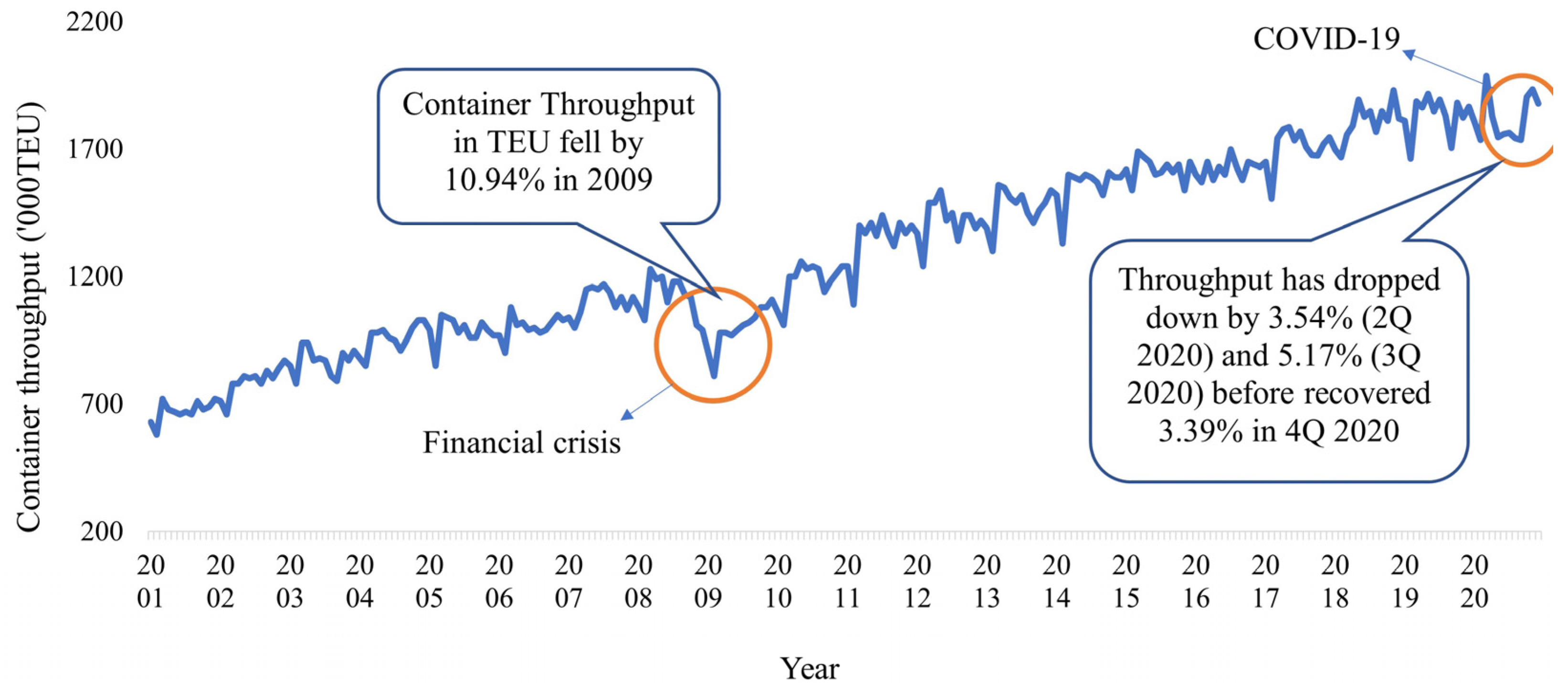The time series data of container throughput show non-stationary characteristics and nonlinear trends, exhibiting highly complex behaviour [1]. Especially in periods of rapid market changes affecting maritime transportation activities and trade, such as the 2009 financial crisis or the COVID-19 pandemic, powerful strategies based on deep learning algorithms will make port performance forecasting more accurate.

Future data forecasts are typically performed using time-series methods that identify trends and cyclic patterns in the dataset, as well as multivariate methods that establish relationships between the variable of interest and other independent variables [27]. The methods, however, do not work well when the dependent variable (demand) exhibits trends, cycles, and dependencies on external disrupting factors. Various methods are used to deal with this situation, including hybrid forecasting methods. This paper presents a novel forecasting method in light of the latest stream of data-driven solutions to operations management problems [28,29,30,31,32]. The proposed algorithm utilizes state-of-the-art sequential machine learning techniques. A hybrid deep learning method is implemented using LSTM and random forest (RF), a machine learning technique derived from decision trees’ structure. An innovative hybrid method is employed to address the problem when there are additional variables or disruptions in the time series. This technique can be used to model both temporal and correlational information in the dataset, whether the data are available in temporal or correlational format. A time-series data model was developed using deep learning techniques, such as LSTM networks. An in-depth discussion of the architecture and data format of LSTM networks is provided, as well as the optimization of hyperparameters. In addition, our method incorporates random forest after LSTM networks in order to improve accuracy and to better understand the demand behaviour by applying key variables. Additionally, the application of the proposed methodology can improve the forecasting performance for the disrupted throughput data in the container ports. The effectiveness of the proposed method was evaluated by a set of performance indexes and statistical significance tests to demonstrate the robust performance of the new proposed approach. Thus, this study addressed the following research questions against disruptions:

-

How to build resilience strategies of container ports using the data analytics method?

-

How to improve port productivity forecasting by utilizing hybrid deep learning methods?

-

How to assess the effectiveness of hybrid forecasting methods using statistical significance tests?

To summarize, the proposed data analytics is based on time series investigation, entropy analysis, Lyapunov exponent, and Hurst exponent, with statistical significance tests. It will help policymakers understand insights into the system dynamics of port throughput and explain the underlying mechanism of port resilience after periods of volatility. In addition, the proposed methods will help port managers evaluate the predictability of port throughput systems, in addition to managerial implications. Next, the paper presents an advanced data analytics method with machine learning to improve prediction accuracy. The novel architecture, data setup, and hyperparameter optimisation have been presented for successful realization of the LSTM method in detail. Moreover, the random forest (RF) algorithm has been implemented as a supervisory method to improve the forecasting accuracy. The rest of this paper is organised as follows: Section 2 presents a literature review; Section 3 presents the resilience analysis using data analytics techniques; Section 4 deals with the forecasting methods using machine learning; in Section 5, the forecasting results, statistical analysis, and discussion are presented to validate the current research findings; finally, Section 6 draws valid conclusions and outlines promising avenues for future research.

2. Literature Review

2.1. Resilience and Dynamic Analysis of the Seaport Operations

Resilience strategies enable the rapid adaptation and efficient restoration of functions in the event of disruptions. The role of different port stakeholders in resilience planning has been examined in recent studies on port resilience [33]; managing supply chain resilience using stochastic modelling [13,20]; resiliency index for maritime transportation systems [34]; vulnerability and resilience of ports to reduce failures and targeted attacks [35]; selection criteria and business attractiveness for port operations [36]; and port capacity bottlenecks [37].

There have been several studies exploring how natural disasters have disrupted container ports in the past. Verschuur and Hall [38] examined 141 disruption incidents across 74 seaports and 27 disasters, with a median duration of 6 days, a 95th percentile of 22 days, and a median disruption duration of 6 days. In a study conducted between 2004 and 2010, Trepte and Rice [37] collected data on 28 incidents of port-related disruptions. The COVID-19 pandemic has recently caused some supply chain disruptions [39,40]. Several unpredictable factors contribute to severe disruptions in supply chain management, affecting its effectiveness and agility [41,42]. It is most likely that they will negatively impact port productivity and performance with delays, because they can lead to complex and undesirable behaviours in system components and transportation services.

There has been an emphasis on describing the underlying mechanisms for cooperation and competition in the port ecosystem and improving the performance of ports through dynamic analysis [41,42]. There is no doubt that nonlinear theory can represent a powerful tool for determining the dynamics of complex systems [17,43,44]. The nonlinear approach has been used very rarely to describe the dynamics of port competitions. Using nonlinear analysis tools to fill the theoretical and practical gap in research is the aim of this paper. In addition to gaining greater insights into nonlinear phenomena in time series data, managers can learn how port ecosystems behave chaotically, with periodicity, stability, and bifurcation.

2.2. Port Productivity Forecasting

Depending on the amount of cargo handled or the number of vessels handled over time, the throughput of a port can be measured. Due to the COVID-19’s dynamic nature and the highly volatile environment in which seaports operate, seaports have to face new market challenges. Identifying whether a system can be forecasted effectively requires an analytic evaluation of seaport characteristics [27]. The forecasting methods widely used among researchers (as a benchmark) and practitioners are genetic algorithms [45]; auto-regressive integrated moving average (ARIMA), with many applications in logistics and supply chain management [46]; exponential smoothing [21]; grey forecasting [23]; and deep learning [24,25,26]. However, container throughput data include non-stationary characteristics and typically show nonlinear behaviours under various disruptions. Therefore, with the traditional forecasting method or regression-type model, it is difficult to achieve the required forecasting accuracy with computational time. Nonlinear and nonstationary time series forecasting approaches have increasingly been investigated in recent years. A novel hybrid decomposition ensemble method was proposed by Niu et al. [47] for describing container transportation volumes. The GP model provided better prediction performance than decomposition methods and SARIMA methods, according to Chen and Chen [48]. The cargo throughput of ships was forecasted using multilayer perceptrons (MLPs) and linear regressions (LRs) by Gosasang et al. [21]. MLP forecasting performed better than the LR model, according to their results.

Machine-learning-based applications are currently used in many different ways [49,50]. Furthermore, deep learning neural networks have been shown to be very effective for solving non-linear sequence learning problems with promising results. Artificial intelligent models and machines are being developed using deep neural networks in deep learning, a new area of machine learning research [45]. For time-series forecasting, RNNs and LSTM networks are widely used, and they outperform popular machine learning methods [20,22]. An RNN or LSTM network retains information across time steps, in contrast to other neural networks [22]. LSTM networks were further improved by Graves, Mohamed and Hinton [51], who created a full-gradient version which overcomes the disappearing gradient problem of LSTM networks. The updating of LSTM networks made it possible for the networks to retain information over long time steps, allowing them to be used for sequence-learning LSTM [51]. Recently, deep learning strategies have been considered as potential schemes for use in several applications, such as CT scans and X-rays using convolutional neural networks (CNNs) and Darknet [52]; detecting noise in ancient images using CNNs [53]; forecasting in multi-channel retailers [27,54]; the financial market [29]; and insurance big data analysis [20]. The combination of many nonlinear transformations and useful expressions are the advantages of deep learning algorithms [27,55].

2.3. Research Gap and Objectives

As pointed out above, there is little empirical evidence regarding port throughput disruption analysis using nonlinear techniques under real-world situations. Real-world systems often have unknown nonlinear structures, which is why several practical systems have been found to have this feature. Using promising nonlinear methods, seaport throughputs have been analysed, but dynamical analysis tools provide policymakers with an understanding of disruption occurrences across different geographical scales [56,57]. Decision-makers can utilize these data analyses to examine how the severity of an event correlates with resilience properties, which could be useful in the risk management of seaports. Furthermore, an empirical evaluation of the predictability of the dataset can be addressed in which the proper forecasting method can be implemented to achieve better performance. The dynamics of port disruptions over time can provide useful insights into supply chain resilience and to evaluate how to recover from disruptions more efficiently using different strategies. In this study, advanced nonlinear analysis methods, including the Lyapunov exponent, Hurst exponent, entropy analysis, and time series analysis, with statistical significance tests, were used to investigate the dynamical behaviour of container throughput to gain a deeper understanding of the disruption mechanisms, as well as the resilience strategies, of port operations. Busan port data were used for quantitative data analysis based on temporal events that have affected system behaviour. Under disruptive events, the port ecosystem becomes a complex dynamical system, which makes the system very difficult to predict using traditional or individual methods. Therefore, this paper proposes a novel hybrid algorithm to improve the prediction accuracy against volatile markets.

3. Empirical Throughput Analysis Using Data Analytics

3.1. Seaport Resilience Analysis—A Case Study of Busan Port (South Korea)

Ecologists first formulated the concept of resilience [9,11]; later, supply chain managers adopted it [58]. The concept of resilience is used in management to describe an organization’s ability to adapt and recover from disruptions. Over the years, research on resilience has expanded to several areas, across the field of logistics and supply chain management [1,14,15,16,37,39,48].

In January 1995, a major earthquake struck near Kobe, Japan. Busan port replaced Kobe port as the biggest trans-shipment hub in northeast Asia until the damaged facilities of Kobe port were fully recovered in March 1997. Currently, Busan port handles almost 75% of total trans-shipments in Korea in 2020 (see Figure 1). Having collected data on container throughput in time series, the initial exercise was to examine the operational sensitivity of Busan port under disruptions. Figure 2 shows the container throughput of Busan port on a monthly basis from January 2001 to December 2020.

A salient example of the challenges is the economic–financial crisis that started in 2008 and lasted until 2009. There has traditionally been a trend for maritime shipping networks to adapt to market volatility by adapting feet capacity [59]. Due to the crisis, there was a surplus of container capacity, particularly on routes from Europe to Asia and the Pacific. There was a 12.4% drop in global container shipping demand in 2009 [60], and then the recovery started in the last six months of 2009, with a recovery rate of 12.61%. This shows that Busan port suffered serious disruptions due to the impact of external factors, but also recovered quickly due to the effective management strategy of the port authority. In the next case, more details about the volatility and recovery rate due to the impact of the COVID-19 epidemic at the beginning of 2020 are depicted in Figure 3.

The COVID-19 pandemic spread around the world by January 2020. Global supply chains are experiencing unprecedented effects as a result of the COVID-19 pandemic [39]. As of April 2020, the Korean government implemented restrictions on maritime trading activities to address the impact of COVID-19 on port operations [60]. More specifically, Figure 3 compares the total volume of containers passing through the port of Busan before the pandemic (in 2018 and 2019) with the fluctuations in port throughput flows after the pandemic outbreak (in 2020). Since April, the amount of container throughput has decreased rapidly after government policies were enacted. Specifically, in April, the growth rate was negative (−1.8%) and bottomed in May (−8.9%); the growth rate remained at negative levels in June, August, August, and September. However, the recovery process appeared to be quite rapid after October 2020, when growth returned to a positive level and was 9.7% higher than the previous month. It is apparent that Busan port is experiencing a very strong but uneven recovery pattern of port operations to cope with the impact of the epidemic. Next, nonlinear time-series analysis deals with the quantitative investigation of observed data (typically univariate). Nonlinear dynamic analysis and statistical methods are used to elucidate the disruption mechanism and the effect of external shocks on the container throughput trend in Busan port.

3.2. Empirical Distribution Analysis

Business decision-making is aided by data analysis techniques that transform time series data into meaningful insights. All container terminals at Busan port are included in the container throughput statistics. For the national transportation market, monthly throughput is calculated using the average volume. According to statistics, volatility is the measure of fluctuations or the dispersion of returns of a process. The variance and standard deviation of returns are often used to calculate throughput volatility in changing business environments. This formula can be used to calculate the monthly return (Rt) and volatility (V) based on the throughput data:

$$R_t=\log (\frac{p_t}{p_{t-1}})$$

(1)

$$V=\sqrt{\frac{{\displaystyle \sum _{t=1}^n{(R_t-\overline{R})}^2}}{n-1}\times \tau }$$

(2)

where p_t and p_t−1 are container throughput in month t and t − 1, respectively; $\overline{R}$ is the mean (average) of monthly returns; and $\tau$ is the length of the time interval set with n data points. Volatility often refers to the amount of uncertainty or risk related to the degree of changes in container throughput. In most cases, the higher the volatility, the riskier the port operations. Using throughput data available in the port management information system (or Korean PORT-MIS), the monthly return of Busan port throughput is illustrated in Figure 4; the monthly volatility is around 6.38%. The empirical results showed that the annual throughput volatility tends to dramatically increase by extending the investigation to the long-term volatility, and the container volume significantly increased from 2001 to 2020; thus, the annual return is very high, accounting for approximately 98.86%. A normal distribution tends to have data points that are close to the mean, as illustrated in Figure 5. The standard deviation is 6.38%, indicating how far throughput returns tend to deviate from the mean when compared with a large deviation from it. Small differences between monthly returns and the mean occur more frequently than large deviations from it, and the standard deviation is less than twice that amount. In order to assist decision-makers in evaluating the underlying mechanisms, as well as predicting the volatility trend, typical dynamical analysis methods were used, as detailed in the following sections.

3.3. Lyapunov Exponents and Dynamical Behaviour

Graphs are commonly used to interpret system behaviour in port and logistics research [54], and quantifiers are commonly used to determine the stability, periodicity, and quasi-periodicity of systems. By calculating some quantifiers, an alternative to graphical time series analysis can be proposed for nonlinear time series analysis [61]. The science of data analytics involves analysing raw data and drawing conclusions based on those conclusions. The Lyapunov exponent (LE), entropy production, fractal dimension, and capacity dimension are some well-known quantifier methods for investigating nonlinear features. Nonlinear features can be demonstrated and classified using the Lyapunov spectrum [62]. In phase space, the LE is derived by calculating the average exponential rates of divergence or convergence of the orbits of nearby satellites based on collected data. Notably, the LE is defined in the manner which is most appropriate to spectral calculations, regardless of how Lyapunov’s spectrum can be determined from different perspectives. It follows that an infinitesimal n-sphere of initial conditions in an n-dimensional phase space will be transformed into an infinitesimal n-ellipsoid over time. The ith LE is defined as follows:

$${\lambda }_i=\underset{t\to \infty }{\lim }\frac{1}{t}{\log }_2\frac{p_i(t)}{p_i(0)}$$

(3)

There is a typical order of largest to smallest [62], in which pi(t) is the length of the ellipsoidal principal axis at time t. Chaos occurs if there is at least one positive LE, or if the largest LE (LLE) exceeds one; otherwise, the system may be stable, periodic, or quasi-periodic [61]. According to this method, the LLE of the port throughput system is plotted in Figure 6. According to the theory formulated in [62], it can be seen that LLE is negative for time series, in which the container throughput behaviour is stable. However, the test results illustrate that the LLE varies greatly at some points in the time series, occurring immediately after external shocks. Due to many doubts about the drastic changes in LLE, the occurrence of large fluctuations in the port system needs to be clarified further. However, deriving the LLE from experimental data is much more difficult. Thus, finding a value for LLE may not be very useful, and the value obtained is usually not very accurate. It is consistent with previous studies that Lyapunov exponents failed to detect some drastic changes within the system. This requires alternative algorithms that are more robust than LE to be able to detect system-specific properties [63]. Therefore, other analytical methods need to be performed to verify the dynamical behaviours of port throughput under the impact of disruptions.

3.4. Entropy Investigation and Complexity

In addition to Lyapunov exponents, entropic measures offer a broader understanding of the nonlinear features of systems [64]. Information entropy is a concept used to measure the complexity and randomness of time series in information theory. The entropy of a dynamical system is determined by the predictability of its dynamical behaviour; thus, more complex systems are less predictable. Entropy computation from finite time series can be complicated with this method. Many methods have been developed to combat this problem, including approximate entropy and sample entropy. However, these approaches have been plagued with weak theories [57]. In contrast, permutation entropy (PE) can efficiently evaluate the dynamic complexity and randomness of arbitrary time series [65]. Based on collected data, the entropic complexity measure is only a function of the probabilities of different states. Based on the relationship of the adjacent values in the time series, its estimation steps are briefly summarized below [57]. For the length of a time series, the m-dimensional vector at time i can be given by

$$X_i^m=\left\{x(i),x(i+\tau ,\dots ,x(i+(m-1)\tau \right\},i=1,2,\dots ,N-(m-1)\tau$$

(4)

where $X_i^m$ denotes the data in new time series, m is the embedding dimension, and $\tau$ is the time delay. As described in [58], $X_i^m$ has permutation ${\pi }_{r_0,r_1,\dots ,r_{m-1}}$, when $X_i^m$ satisfies the following condition:

$$x(t+r_0\tau )\le x(t+r_1\tau )\le \dots \le x(t+r_{m-1}\tau )$$

(5)

where $0\le r_i\le m-1$ and $r_i\ne r_j$. It can be derived from Equation (5) that an m-tuple vector has m! possible distributions. Moreover, the calculation of frequency of distribution is given as

$$P(i)=\frac{Num\left\{X_i^m\right\}}{N-(m-1)\tau }$$

(6)

where $Num\left\{X_i^m\right\}$ represents the number of $X_i^m$, and it is consistent with the type $\pi$. Then, the PE with m-dimensions can be described as

$$H_{PE}(m)=-{\displaystyle \sum _i^{N-(m-1)\tau }P(i)\ln (P(i))}$$

(7)

Notably, when $P(i)=\frac{1}{m}!$, $H_{PE}$ reaches the maximum value $\ln (m!)$. The PE value can be normalized through $\ln (m!)$ as

$$H_{NPE}(m)=\frac{H_{PE}(m)}{\ln (m!)}$$

(8)

In addition, the entropy value $H_{NPE}(m)$ is measured between 0 and 1. The smaller $H_{NPE}(m)$ value offers more periodicity and regularity in the time series. To investigate the resilience strategy of the port throughput system mentioned in Section 3.1, the PE method is also applied to clarify the dynamic behaviour of the throughput trend. In the dataset, the numbers of training and test samples are 192 and 48 data points, respectively, where the data length N is given as 240. As illustrated in Figure 7, the basic properties of entropy can be described by the port throughput. First, it is a concave function, and the entropy value is 0 when t = 0, because the variable is not random. In the next period, $H_{NPE}$ spiked to 0.6 when t = 5, and then moved mostly sideways for the next few cycles before continuing to rise sharply. From t = 75, the PE hit a value of 1 and retained that pattern until the end of the period. The test results can be explained by exploring the operating history of Busan port. The internal factors are always changing depending on such as operating procedures, management policies, and constantly changing infrastructure, which make the trend of the container throughput fluctuate greatly. In addition, external shocks disturb the port operations, especially complex disruptions such as the financial crisis and the COVID-19 pandemic. Thus, information entropy can be said to be a measure of the systematic ordering degree or randomness of the time series. Through the entropy analysis, the port throughput of Busan port shows complex dynamic behaviour.

Next, the permutation entropy was used to investigate the port performance over a 3-year time period (2018–2020), and the short-term results are illustrated in Figure 8. At the beginning of the examination, $H_{NPE}$ reached a low value every year. However, towards the end of the period, $H_{NPE}$ increased significantly and approached $H_{NPE}\approx 1$ for 2020, whereas these values were relatively low in 2018 and 2019. The higher $H_{NPE}$ value in 2020 is explained below. Under the impact of the COVID-19 pandemic, Busan port has been facing various challenges in cargo handling activities and shipment services, affecting the dynamic behaviour of seaport operations. With the entropy analysis and its resulting explanation, it can be seen that the throughput system of Busan port exhibits a highly complex, nonstationary, and high level of randomness, especially in 2020 (a period of great disruption and recovery).

3.5. Predictability with Hurst Exponent and Fractal Dimension

There are many types of perturbations that can affect port management systems, such as time delays, internal uncertainties, external shocks, and feedback processes between entities. Quantitative analysis of time series can reveal nonlinearity, complexity, and chaos using the approaches mentioned. The Hurst exponent is robust, efficient, and requires few assumptions about underlying mechanisms, and is appropriate for many applications, from finance to logistics [66,67]. A Hurst exponent measures the long-term memory of time series data and is used in fractal analyses [68]. As a function of the time span of a time series, the Hurst exponent (H) determines the asymptotic dynamics of a rescaled range. Rescaled range analysis (R/S analysis) can be performed based on the collected data. The steps for R/S analysis of time series data are as follows:

$$\mu =\frac{1}{N}{\displaystyle \sum _{i=1}^N{X}_i}$$

(9)

Evaluate the mean adjusted series Y,

$$Y_t=X_t-\mu ,\hspace{0.17em}t=1,2,\dots \mathrm{N}$$

(10)

Calculate the cumulative deviate series Z,

$$Z_t={\displaystyle \sum _{i=1}^N{Y}_i},\hspace{0.17em}t=1,2,\dots \mathrm{N}$$

(11)

Determine the range series R,

$$R_t=\max (Z_1,Z_2,\dots Z_t)-\min (Z_1,Z_2,\dots Z_t),\hspace{0.17em}t=1,2,\dots \mathrm{N}$$

(12)

Compute the standard deviation series S,

$$S_t=\sqrt{\frac{1}{t}{\displaystyle \sum _{i=1}^t{(X_i-u)}^2}},\hspace{0.17em}t=1,2,\dots N$$

(13)

where u is the mean value from X₁ to X_t. The rescaled range series can be given as

$${(R/S)}_t=\frac{R_t}{S_t},\hspace{0.17em}t=1,2,\dots N$$

(14)

Notably, (R/S)_t is averaged values over the ranges [X₁, X_t], [X_t+1, X_2t] until [X_(m−1)t+1, X_mt], where m = [N/t]. In practice, to use all data for calculations, a value of t is chosen such that it is divisible by N. The connection between (R/S)_t and the Hurst exponent (H) is calculated by

$${(R/S)}_t=c_{\alpha }{t}^H$$

(15)

where c_α is a constant. A plot of (R/S) versus t in log axes is used to estimate the Hurst exponent, followed by an estimation of the slope of the curve using an ordinary least squares (OLS) method. Higher values indicate a smoother trend, less volatility, and less roughness, whereas lower values indicate a more random walk (H = 0.5). A time series can be classified in the following categories: H = 0.5 represents a random distribution indistinguishable from noise or disturbance; 0 < H < 0.5 indicates that the system behaviour is a mean-reverting and anti-persistent series (more chaotic); and 0.5 < H < 1.0 shows that the system tends to a persistent series (less chaotic or trending).

In Figure 9, the Hurst exponent is illustrated for a sliding window of length 140. Overall, there is a significant difference between 0.5 and the Hurst exponent in Busan port’s container throughput, which indicates that loading and unloading operations have a distinct long-term memory effect on container volume. The dynamic features demonstrate the following: (1) The port throughput volume is not only affected by the shipping market with external disruption, but is also influenced by past and present throughput volumes; (2) The Hurst exponent is higher than 0.5 under long time series with many environmental shocks such as financial or pandemic crises, which indicates that the trending pattern on the throughput volume is strong and the trend will continue in the port operation system [60]. If the volume of container throughput is lower than the average volume of throughput at a certain time period, it means that the throughput tends to be lower at the next time point, whereas if the container throughput is higher than average, it means that the volume of container throughput tends to be higher over time; (3) The port authority and decision-makers of the port operation system could combine the previous interevent time distribution with the present situation and use analytical and statistical methods to improve the operation and management efficiency for port productivity.

4. Deep Learning Approach for Port Productivity Forecasting

Based on the data analytics discussed above, the nature and dynamics of container throughput of Busan port are a complex and nonlinear time series, containing uncertain factors; especially, it is also influenced by many external disturbances. Therefore, building a robust forecasting method is necessary so that decision-makers can rely on it for improving operational efficiency as well as mitigating external shocks, thereby sustaining the growth trend and productivity of port operations. For predicting port throughput, LSTM networks have been shown to be highly effective in time-series forecasting tasks [27,29]. The dataset contains several throughput patterns during some volatile periods of international shipping. Therefore, a prediction model based on LSTM is a suitable alternative to handle linear and non-linear data, as well as data fluctuations caused by disruptions. This is the limitation of the LSTM model applied to a highly volatile market caused by external factors. Therefore, random forest (RF) is proposed as a complementary method to mitigate residual errors from the LSTM scheme. Multiple regression could be employed; however, RF is considered due to its superiority over others in prediction accuracy, with wide applicability in supply chain management [31,54]. In addition, recent empirical evaluations of the RF strategy show the strategy to be a very competitive advantage when it comes to forecasting performance [27,29,54].

4.1. LSTM Algorithm

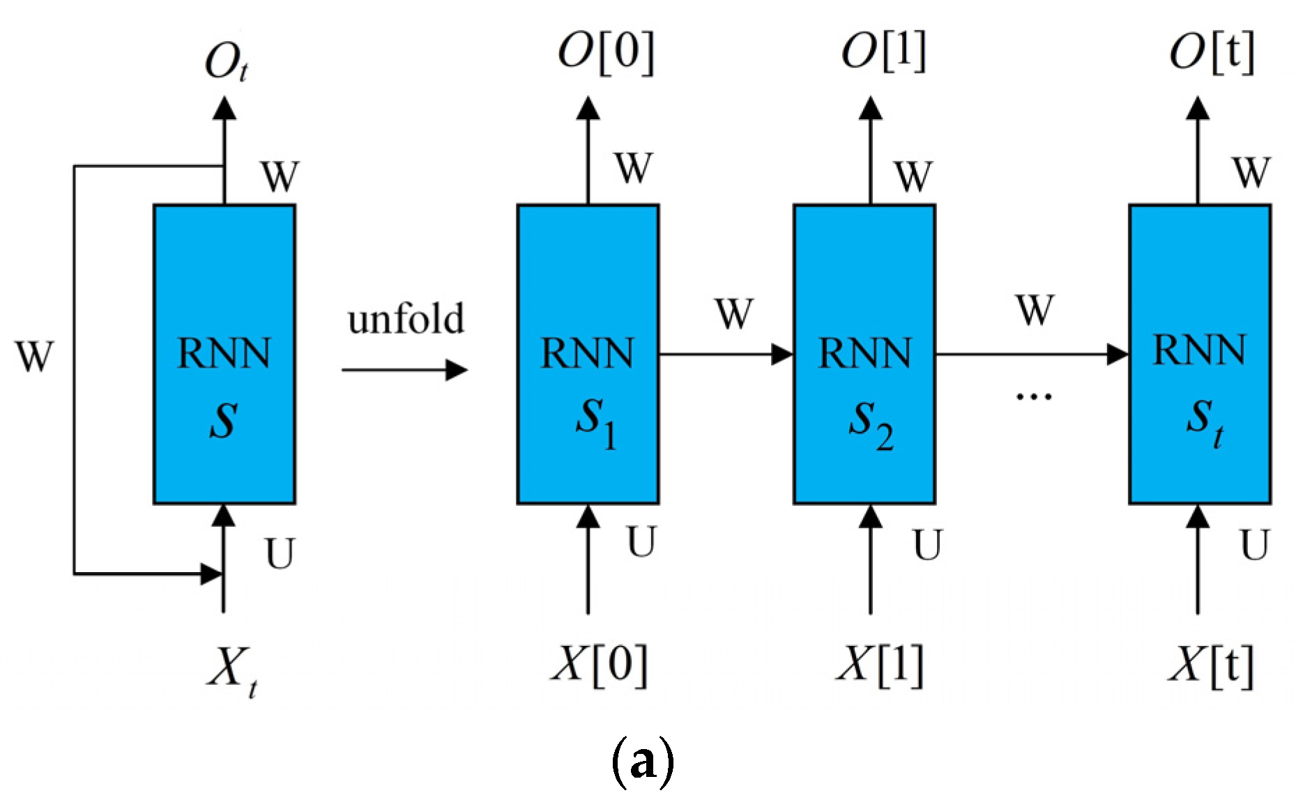
In artificial recurrent neural networks (RNNs), LSTM networks are among the most popular [29,69,70,71]. In time series analyses, RNNs are excellent because they consider the relationship between previous and subsequent data. As with normal neural networks, RNNs are trained by backpropagation and then learn by gradient descent [27]. Recurrent neural networks recirculate input data according to layers, in contrast to normal neural networks. In this way, new information is added to the memory and past information is remembered. A generic RNN architecture is shown in Figure 10a: X[0], X[1]…X[t] are the data inputs, and O[0], O[1]…O[t] are the data outputs, where t is the time or order for each vector [51].

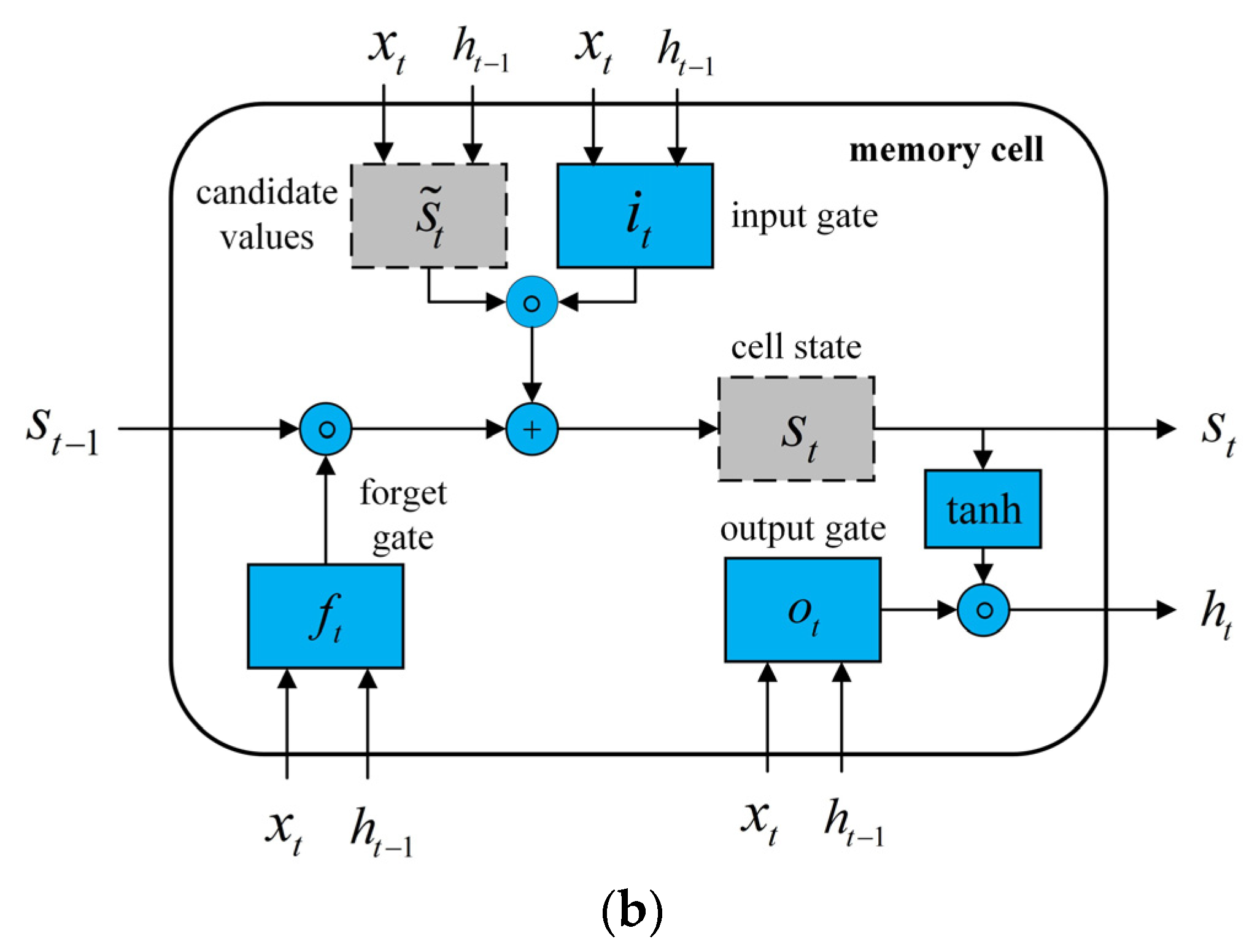
There are three basic layers in LSTM networks: an input layer, one or more hidden layers, and an output layer. Feature space (explanatory variables) is equal to the number of neurons in the input layer. In the hidden layer(s) of LSTM networks, memory cells play a key role in describing their characteristics [51]. Figure 10b illustrates the structure of a memory cell. LSTM layer memory cells are updated at every time step t according to the equations below. The notations used here are as follows:

• $x_t$ is the input vector at time step t.
• $W_{\mathrm{f},\mathrm{x}},\hspace{0.17em}{W}_{\mathrm{f},\mathrm{h}},\hspace{0.17em}{W}_{\tilde{\mathrm{s}},\mathrm{x}},\hspace{0.17em}{W}_{\tilde{\mathrm{s}},\mathrm{h}},\hspace{0.17em}{W}_{\mathrm{i},\mathrm{x}},\hspace{0.17em}{W}_{\mathrm{i},\mathrm{h}},\hspace{0.17em}{W}_{\mathrm{o},\mathrm{x}}$ and $\hspace{0.17em}{W}_{\mathrm{o},\mathrm{h}}$ are weight matrices.
• $b_f,\hspace{0.17em}{b}_{\tilde{s}},\hspace{0.17em}{b}_i$, and $b_o$ are bias vectors.
• $f_t,i_t$, and $o_t$ are vectors for activating the respective gates.
• $s_{\mathrm{t}}$ and ${\tilde{s}}_t$ are vectors for the cell states and candidate values, respectively.
• $h_t$ is a vector representing the LSTM layer.

Therefore, the activation values f_t of the forget gates at time step t are computed based on the current input x_t, the outputs h_t−1 of the memory cells at the previous time step (t − 1), and the bias terms b_f of the forget gates:

$$f_t=sigmoid(W_{f,x}{x}_t+W_{f,h}{h}_{t-1}+b_f)$$

(16)

In the second step, the LSTM layer determines which information should be added to the network’s cell states ($s_{\mathrm{t}}$). This procedure comprises two operations:

$${\tilde{s}}_t=\tanh (W_{\tilde{s},x}{x}_t+W_{\tilde{s},h}{h}_{t-1}+b_{\tilde{s}})$$

(17)

$$i_t=sigmoid(W_{i,x}{x}_t+W_{i,h}{h}_{t-1}+b_i)$$

(18)

In the third step, s_t is calculated based on the results of the previous two steps:

$$s_t=f_t\circ s_{t-1}+i_t\circ {\tilde{s}}_t$$

(19)

In the last step, the outputs of h_t are derived in the following two equations:

$$o_t=sigmoid(W_{0,x}{x}_t+W_{0,h}{h}_t+b_0)$$

(20)

$$h_t=o_t\times \tanh (s_t)$$

(21)

LSTM networks process input sequences by displaying their features timestep by timestep. The network processes the input (in this case, one single standardized return) at each time step t, as given in the equations above. The final output is returned once all elements of the sequence have been processed.

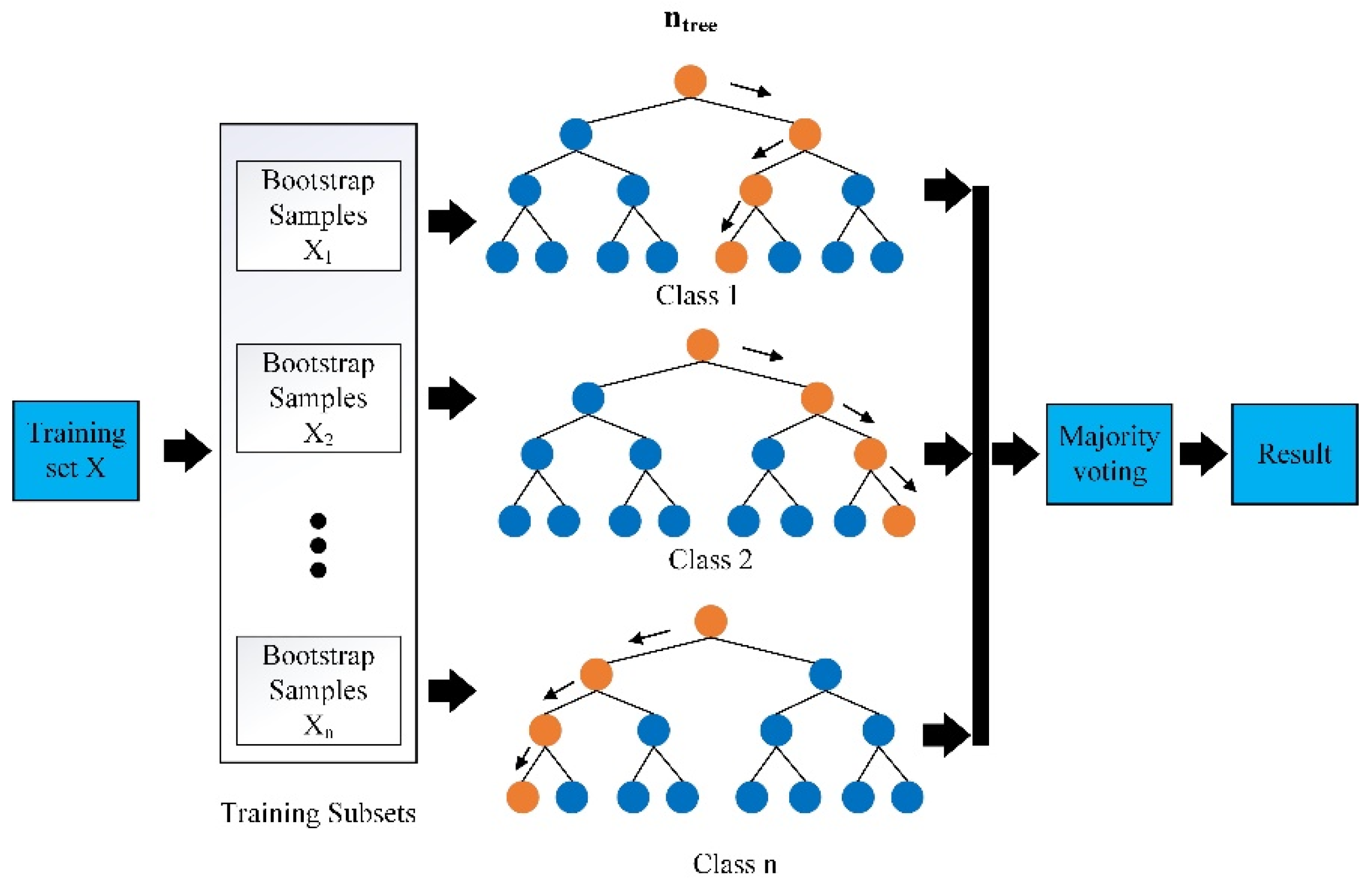
4.2. RF Algorithm

In decision tree modelling, the random forest (RF) algorithm is based on an ensemble classifier. A bootstrap sampling approach is used to generate n training data subsets from an original dataset. These subsets are then trained to build n decision trees [72]. A combination of decision trees is used in the RF algorithm to overcome this shortcoming. When multiple trees are combined, the average of multiple trees will produce the correct results, eliminating the instability of a single tree [72,73]. The final classification result is determined based on the votes for each sample of the testing dataset (Figure 11). Throughput forecasts are performed using RF, with explanatory variables as input variables and residuals from stage 1 as dependent variables [27]. The proposed tasks would be easier to solve with multiple regression; however, RF is superior in accuracy and has wide applicability, including in retail management [27,54], financial management [29], and supply chain management [31]. Furthermore, recent empirical evaluations of the RF strategy demonstrate competitive forecasting performance. Due to the large number of trees, it is computationally expensive.

4.3. Hybrid Deep Learning for Forecasting Strategy

Batch size in the LSTM is defined as a set of past values used to predict future values. Batch size ranges from a single sample to a whole training set, but smaller batch sizes enable computing resources to be optimized. In this way, LSTM cannot make use of the data that are available across products to train the model. In contrast, RF can be trained over datasets on all products, thus obtaining more data and obtaining a better model for predicting the relationship between demand and independent variables; however, RF cannot detect trends or cyclicity in demand [27]. As a result, the proposed method, based on the three-step approach outlined below, overcomes these limitations and presents a complete solution to the problems of modelling the temporal and regression effects of port throughput data.

Combining LSTM with RF enables the proposed forecasting method to take advantage of both methods’ complementary strengths, while avoiding overlapping weaknesses. Thus, the proposed method is the hybrid cooperative schemes from steps (1) and (2). In step (1), LSTM acts as the main algorithm to predict the nonlinear time series. In step (2), RF acts as a supervisory algorithm to predict the errors of step (1); then, step (3) can be used for the final forecasting results. These are errors caused by external shocks as well as serious internal uncertainties that LSTM cannot cover. Thus, the complete algorithm works in this way:

Step (1): The data series X_t is an input of the LSTM network, and forecasting $\widehat{y}$, and the errors $e_{LSTM}=y-\widehat{y}$ are typically generated. The forecasting step (1) is presented in Algorithm 1.

Step (2): The residuals from the first forecast $e_{LSTM}$ are regressed over independent variables through the RF model and forecasting ${\widehat{e}}_{LSTM}$ values for the residuals are determined. This algorithm step can be described in Algorithm 2.

Step (3): The final forecasting is obtained as: $y_F=\widehat{y}+{\widehat{e}}_{LSTM}$

Due to its ability to overcome both LSTM and RF limitations, the hybrid method should be able to predict outcomes better than either algorithm individually. LSTM forecasts future values based on past data, called the batch size. Smaller batch sizes produce better results when compared with larger batch sizes. Therefore, the algorithm cannot be used to train the model based on data from another dataset. Conversely, RF can be trained as a function of data from all training datasets; thus, it has a larger dataset on which to operate. Demand data cannot be modelled using RF, however, because they lack trend and cyclicity. In this regard, a hybrid approach that takes advantage of the combined advantages through three forecasting steps is suggested to overcome those limitations and provide a comprehensive solution to model the temporal and regression effects of demand data [27,29].

Algorithm 1: Forecasting base on LSTM architectures
$\mathrm{Input}: \mathrm{Data}\mathrm{input}{\mathrm{x}}_t$, training data length Ly, an LSTM model with P layers, weight W, and training epoch n			Dataset to be used
$\mathrm{Output}: \mathrm{Predicted}\mathrm{throughput}\widehat{y}$$\mathrm{and}\mathrm{error}{e}_{LSTM}$
1.	$\mathrm{Set}n=0,y(n)=y_0$		${}_{⊳}$ Training data
2.	$\mathrm{while}t<L_y$, do
3.		$t\leftarrow t+1$
4.		$f_t=sigmoid(W_{f,x}{x}_t+W_{f,h}{h}_{t-1}+b_f)$	${}_{⊳}$ LSTM input
5.		${\tilde{s}}_t=\tanh (W_{\tilde{s},x}{x}_t+W_{\tilde{s},h}{h}_{t-1}+b_{\tilde{s}})$	${}_{⊳}$ input gate
6.		$i_t=sigmoid(W_{i,x}{x}_t+W_{i,h}{h}_{t-1}+b_i)$	${}_{⊳}$ forget gate
7.		$s_t=f_t\circ s_{t-1}+i_t\circ {\tilde{s}}_t$	${}_{⊳}$ cell
8.		$o_t=sigmoid(W_{0,x}{x}_t+W_{0,h}{h}_t+b_0)$	${}_{⊳}$ output gate
9.		$h_t=o_t\ast \tanh (s_t)$	${}_{⊳}$ LSTM output
10.		$v_t=h_t(y_t)$
11.	end
	Prediction results:
12.	$E=AP(v^t,v^{t-1},v^{t-2},\dots ,v^{t-M})$		${}_{⊳}$ Average Pooling
13.	$\mathrm{Compute}{P}_k=\left\{P_1,\dots ,P_K\right\}\leftarrow soft\max (E)$
14.	$\mathrm{Find}Id\mathrm{x}\leftarrow Support(\max (P_k))$		${}_{⊳}$ Index of highest probability
15.	$\widehat{y}=Id\mathrm{x}$		${}_{⊳}$ Predicted output
16.	$e_{LSTM}=y-\widehat{y}$		${}_{⊳}$ Predicted error
17.	End procedure

Algorithm 2: Error forecasting using the RF method
$\mathrm{Input}\text{:} \mathrm{error}\mathrm{dataset}\mathrm{for}\mathrm{training}{e}_{LSTM}=y-\widehat{y}$						${}_{⊳}$ dataset to be used
$\mathrm{Output}: \mathrm{Predicted}\mathrm{error}{\widehat{e}}_{LSTM}$
1.	$n\_repl\leftarrow 240$					${}_{⊳}$ number of replicate experiments
2.	$n\_folds\leftarrow 20$					${}_{⊳}$ number of cross-validation folds
3.	$n\_runs\leftarrow 50$					${}_{⊳}$ number of runs per fold
4.	$n\_trees\leftarrow 100$					${}_{⊳}$ number of trees in RF
5.	$\mathrm{for}repl\leftarrow 1$$\mathrm{to}n\_repl$ do
6.		$\mathrm{Shuffle}\mathit{dataset}\mathrm{and}\mathrm{generate}n\_folds$ folds
7.		for $folds\leftarrow 1$$\mathrm{to}n\_folds$ do
8.			Split dataset into training and test sets according to fold
9.			$jungle=\left\{\right\}$			${}_{⊳}$ initialize empty jungle
10.			$\mathrm{super}\text{-}\mathrm{ensemble}=\left\{\right\}$			${}_{⊳}$ initialize empty super-ensemble
11.			for run ← 1 to n_runs do
12.				Train RF with n_trees on training set
13.				Test resultant RF on test set
14.				Add all models (decision trees) to jungle
15.				Add RF to super-ensemble
16.			end
17.			Test jungle
18.			Test super-ensemble
19.			Generate gardens of given sizes using order-based pruning, clustering-based pruning, and lexigarden
20.			Test resultant gardens on test set
21.		end
22.	end

5. Empirical Testing Results

5.1. Experimental Setup

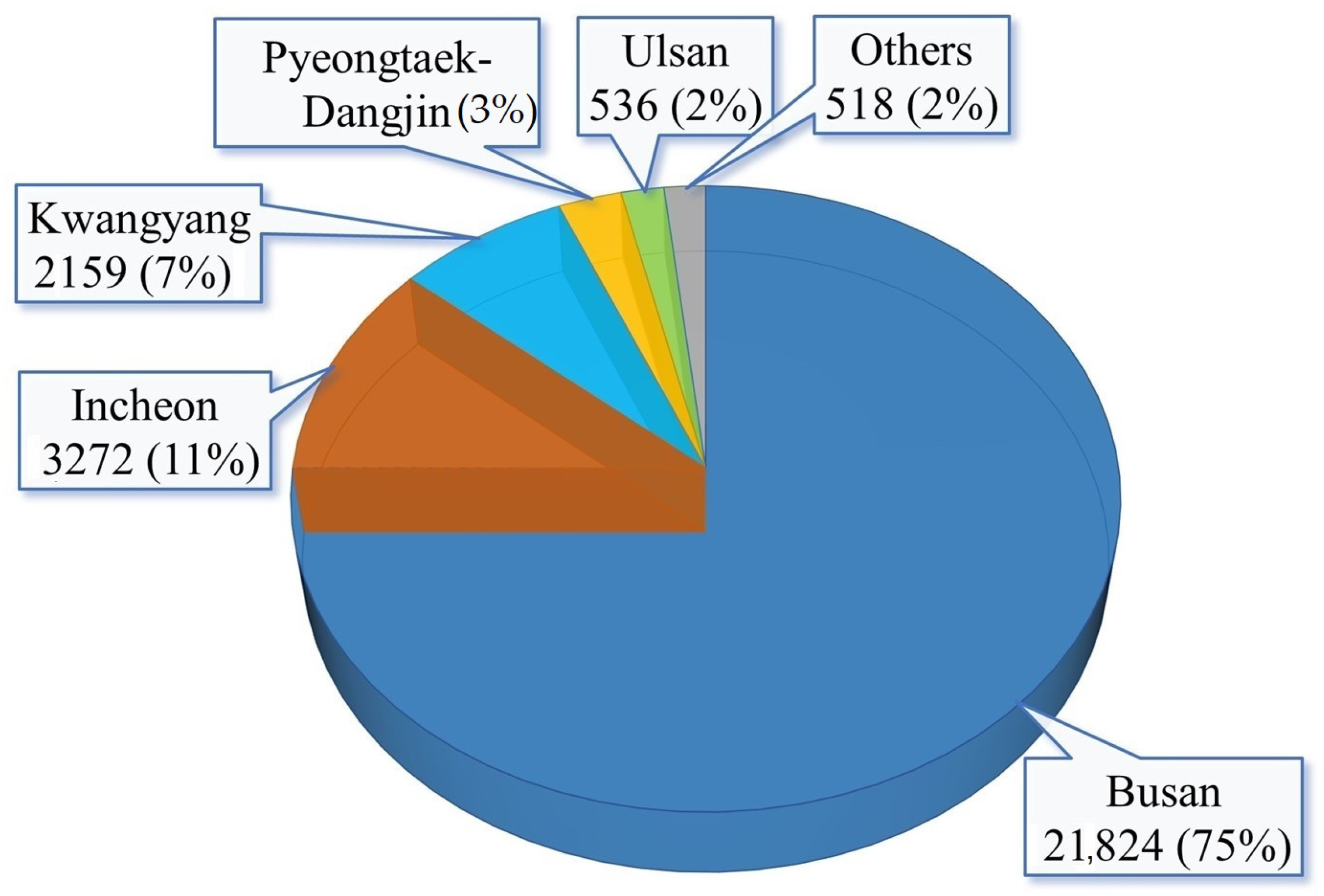
The strategic vision for Busan port has been about ensuring connectivity, productivity, and competitiveness. The dataset was derived from container throughput, which can be expressed as a twenty-foot equivalent unit (TEU) of Busan port in the period of 2001M1 to 2020M12, available in the shipping port logistics information system (PORT-MIS). The monthly data included 240 data points and covered import, export, and trans-shipment containers (

Table 1. Summary statistics of the dataset (million TEU).

Mean	Standard Error	Median	Mode	Standard Deviation	Minimum	Maximum	Sum
1.29	0.02	1.24	0.99	0.37	0.58	1.99	310.68

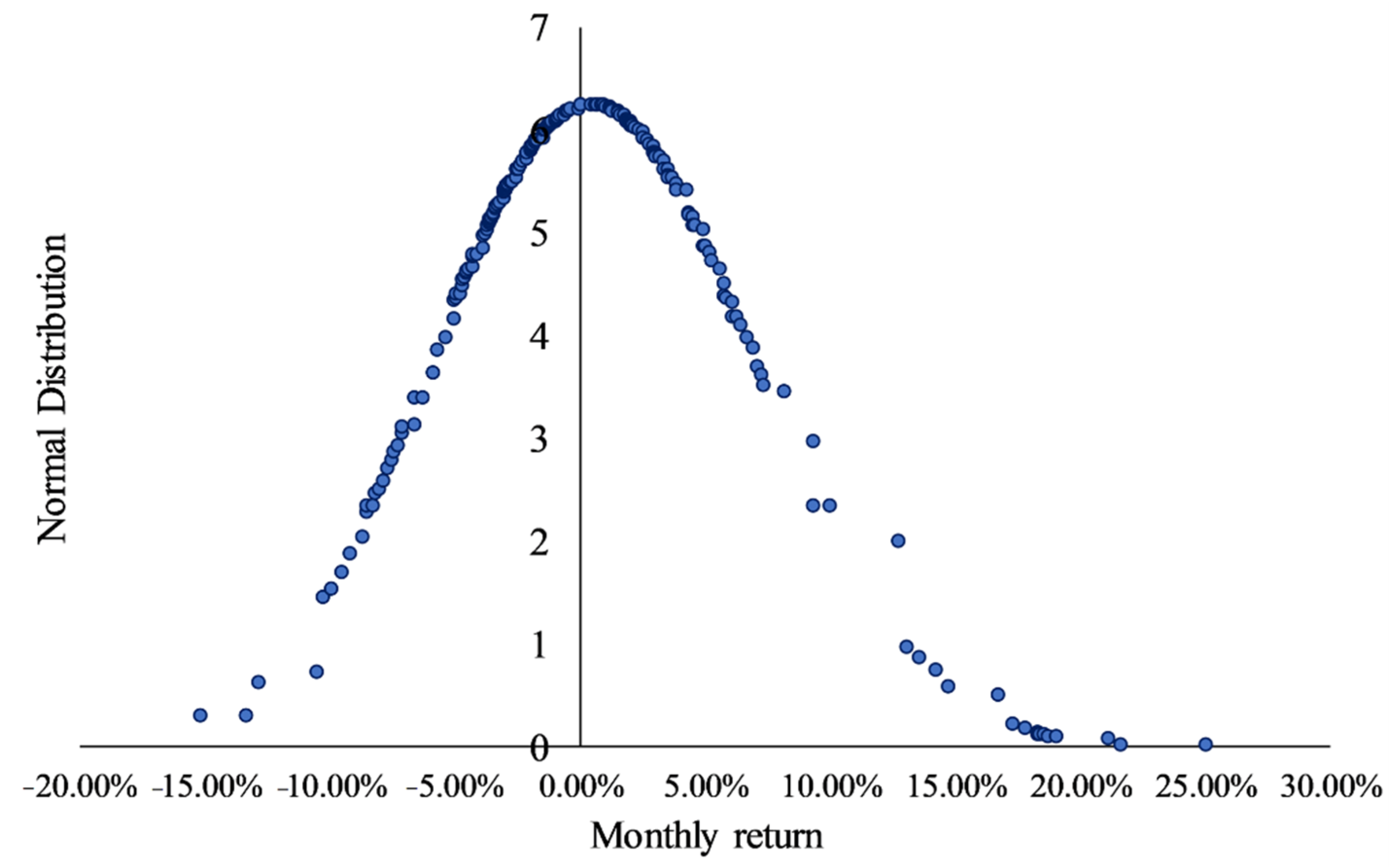
). The same training and testing datasets were used for all testing methods. The training dataset ranged from 2001M1 of monthly data to 2016M12, including 192 data points; the testing dataset included 48 data point consisting of monthly data from 2017M1 to 2020M12. According to the analysis in Section 3.2, the dataset (training and testing) followed a normal distribution, and the monthly volatility was around 6.38%.

Two convolutional layers of 64 and 128 filters were used in the RNN and LSTM models, respectively. Using a max pooling layer of 2 and an LSTM layer of 120 units, a fully connected layer of 36 neurons, and a neuron as the output layer, each layer was followed by a max pooling layer. There were 100 runs performed per fold for each training set of 4 folds and the left-out test set of 4 folds. A 100-tree RF was fitted for the training set, and a test set was created from the fitted RF. In addition, all trees were collected into a jungle and all RFs were saved into a super-ensemble.

5.2. Forecasting Performance Criteria

In order to determine a proposed algorithm’s predictive capabilities, four criteria are commonly used: mean squared error (MSE), mean absolute error (MAE), root-mean-square error (RMSE), and root-mean-square logarithmic error (RMSLE). The metric of each method is described in Equations (20)–(25), respectively. MSE, MAE, and RMSE are three well-known statistical measures. These methods were performed in this study for evaluating the deviations of forecasted results from actual values. MSE measures the difference between the original and forecasted values extracted by squaring the average difference over the dataset. MAE represents the deviations of the original and forecasted values extracted by averaging the absolute difference over the dataset. RMSE is obtained by the square root of MSE.

$$MSE=\frac{1}{N}{\displaystyle \sum _{i=1}^N{(y_i-{\widehat{y}}_i)}^2}$$

(22)

$$MAE=\frac{1}{N}{\displaystyle \sum _{i=1}^N(\left|y_i-{\widehat{y}}_i\right|})$$

(23)

$$RMSE=\sqrt{\frac{1}{N}{\displaystyle \sum _{i=1}^N{(y_i-{\widehat{y}}_i)}^2}}$$

(24)

$$MAPE=\frac{1}{N}{\displaystyle \sum _{i=1}^N\left|\frac{y_i-{\widehat{y}}_i}{y_i}\right|}$$

(25)

$$RMSLE=\sqrt{\frac{1}{N}{\displaystyle \sum _{i=1}^N(\log {({\widehat{y}}_i+1)}^2-\log {(y_i+1)}^2)}}$$

(26)

where $y_i$ and ${\widehat{y}}_i$ are the actual and forecasted values, respectively, and N is the sample size.

A modern statistic evaluation method, the Diebold–Mariano (DM) test, is presented in this paper instead of the traditional evaluation criteria for forecasting performance mentioned previously [74], which can be used as a quantitative tool to assess forecast accuracy. Using this test, it is possible to determine whether the difference between the forecasts is significant or the result of a specific choice of datasets. According to Diebold and Mariano [75], the DM test theory originated from them. In fact, the DM test tends to reject the null hypothesis too often for a dataset with a small sample size. A better test procedure is based on the Harvey et al. [69], or the so-called HLN test method, which is described as follows:

$$HLN=DM\sqrt{\frac{T+1-2h+h(h-1)}{n}}$$

(27)

The DM test has been widely used to test for forecast accuracy in large samples. If the forecast samples are small, the HLN test is conveniently used, which is actually a modification of the DM test with a small sample size. In this study, both DM and HLN test methods were used to evaluate the effectiveness of the proposed forecasting algorithms.

5.3. Long-Term Forecasting Results for Container Throughput

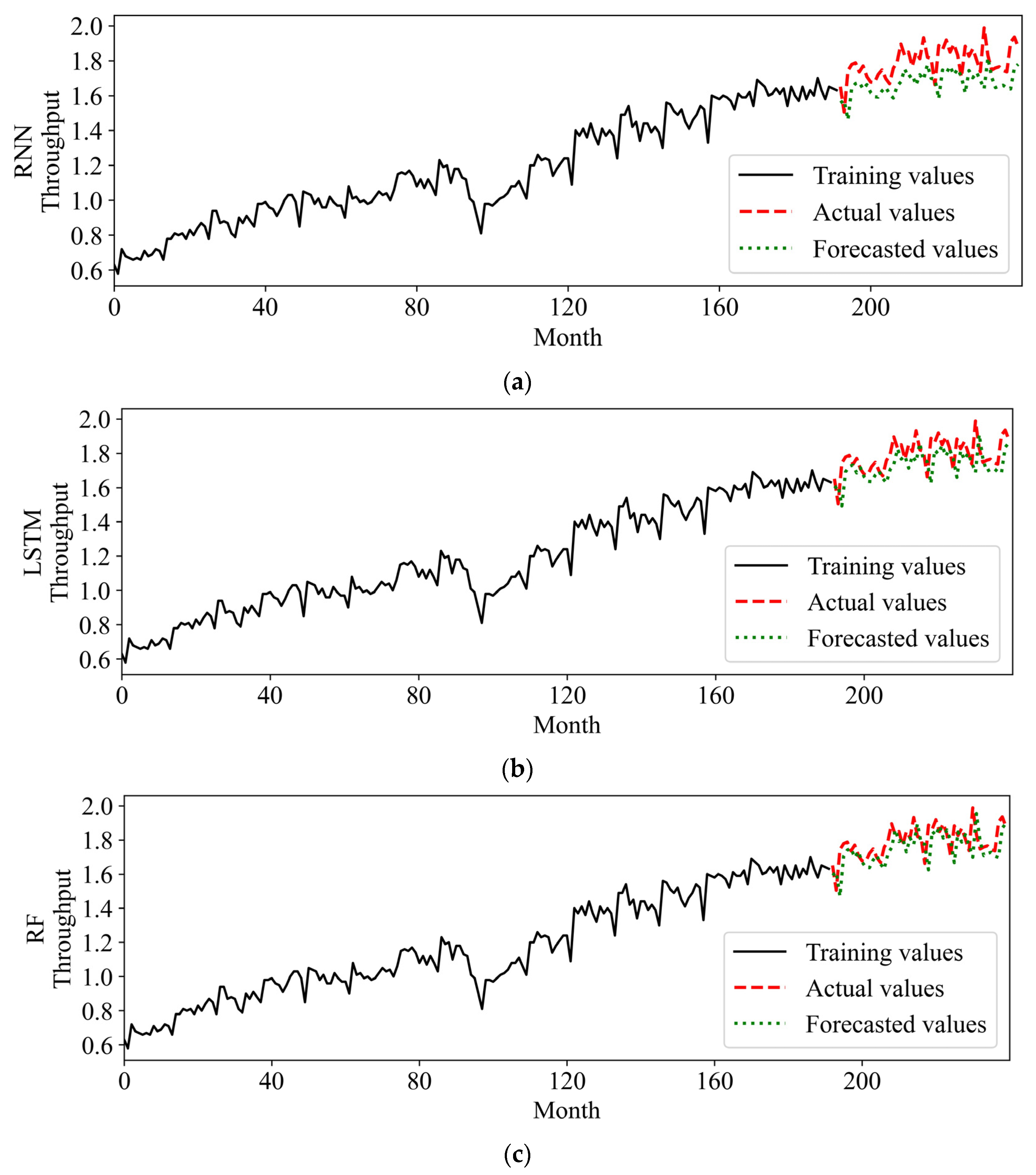
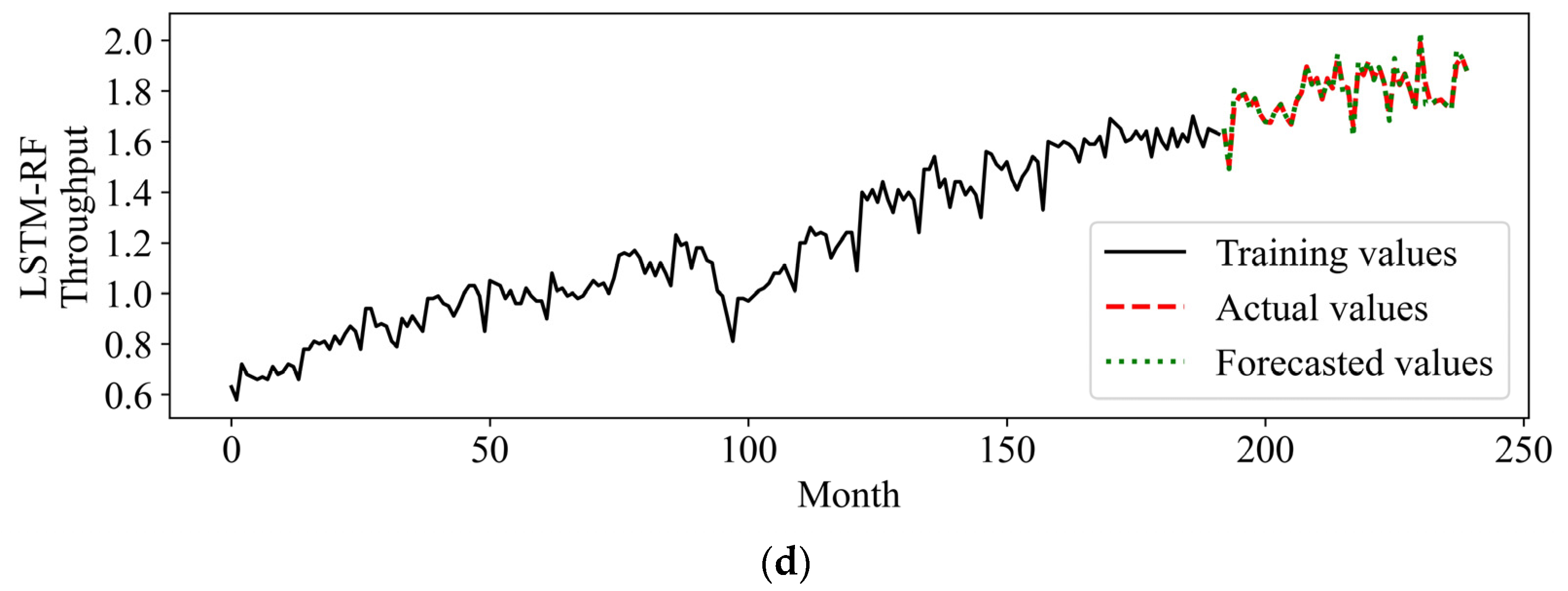
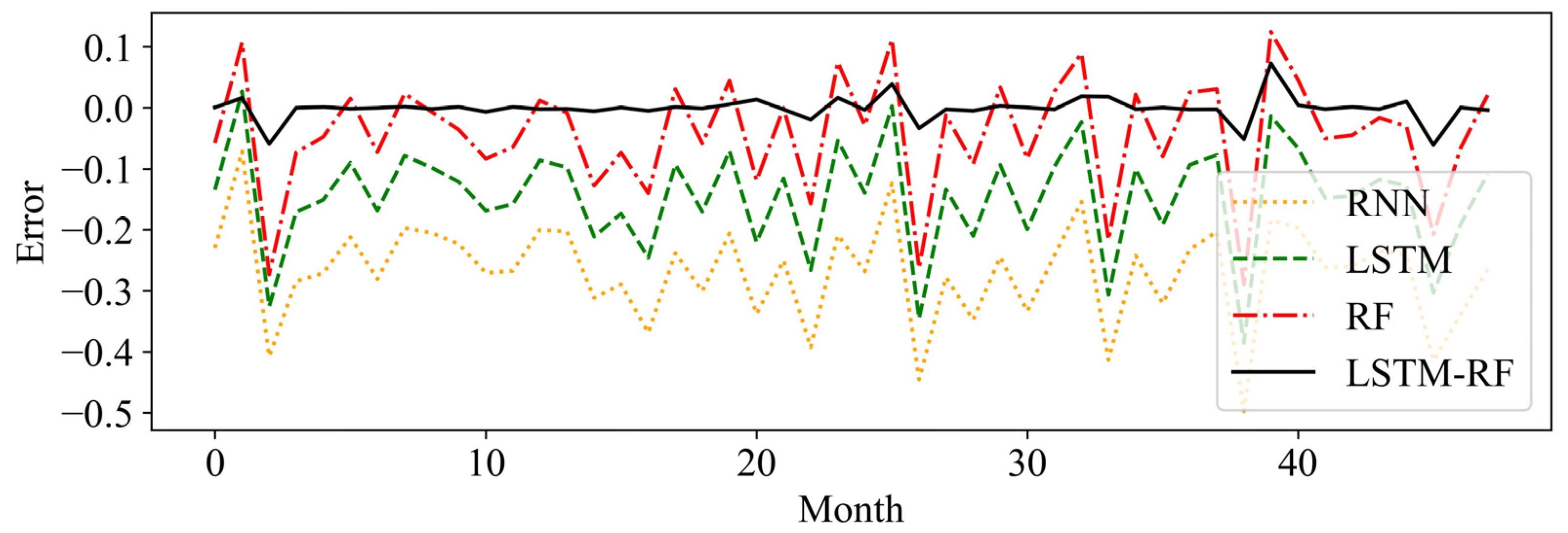
The proposed forecasting method was initially applied for long-term prediction. A forecast of the container throughput volume for the next four years was based on data from the first 16 years for training. Three benchmarking algorithms, RNN, LSTM, and RF, were used to evaluate the effectiveness of the proposed algorithms. The actual extrapolations are shown in Figure 11. It can be seen in Figure 11 that LSTM, RF, and the proposed methods achieved better forecasting performance than RNN. Moreover, the results show that the new hybrid approach has the best performance where the forecasting data series could converge to the actual data. In more detail, the residual errors of the forecasting methods are shown in Figure 12. It can be seen that the proposed method performs extremely well compared with other methods, whereas the RNN algorithm yields relatively larger errors than other methods (see Figure 13).

As shown in

Table 2. Long-term forecasting performance evaluation (the smaller, the better).

	MAE	MSE	RMSE	MAPE	RMSLE
RNN	0.0115	0.0797	0.1075	0.0436	0.0388
LSTM	0.0277	0.1426	0.1664	0.0784	0.0610
RF	0.0093	0.0741	0.0966	0.0412	0.0348
LSTM-RF	0.0004	0.0094	0.0190	0.0051	0.0066

, throughput forecasts for the next four years are averaged. Results from the proposed method show that forecasts are more accurate. When comparing all methods for forecasting port throughput, the proposed hybrid method outperforms benchmarking methods.

Based on the DM and HLN tests, statistical significance tests were conducted for the empirical evaluation differences between the proposed hybrid method and the aforementioned algorithms (

Table 3. Long-term prediction (4 years in the future) with statistical significance tests.

	A: DM Test (p-Value)				B: HLN Test (p-Value)
Algorithm (i,j)	Proposed	RNN	LSTM	RF	Proposed	RNN	LSTM	RF
Proposed	-	0.0000	0.0000	0.0000	-	0.0000	0.0000	0.0000
RNN		-	0.2631	0.1479		-	0.2209	0.1156
LSTM			-	0.0000			-	0.0000
RF				-				-

). Statistically significant differences in forecasting performance exist at a 95% confidence level between the proposed method and different benchmarking methodologies. For the null hypothesis that paired methods have equal performance, panel A of Table 3 shows the p-values from the DM test. A p-value indicates the confidence that method i will produce a worse prediction than method j. Forecasts using the proposed method are superior to benchmarking methods (RNN, LSTM, and RF) because all individual hypotheses are rejected over the 95% significance level. As shown in Table 3, the HLN test yielded similar results for panel B. Comparing the proposed algorithm with other algorithms, all test results demonstrated optimal performance. Therefore, this hybrid method can be successfully applied for throughput forecasting in a volatile environment with ensuring better performance and higher accuracy compared with conventional methods.

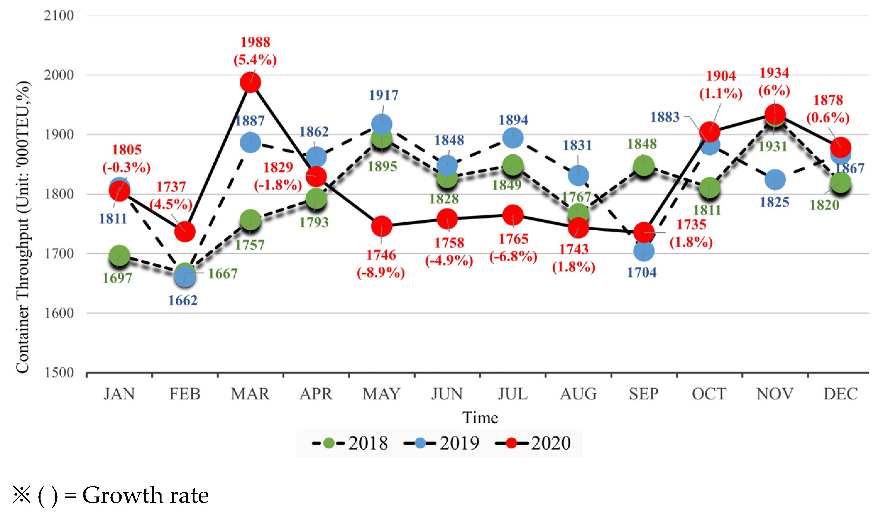
5.4. Short-Term Forecasting Results for Container Throughput

After evaluating long-term forecasting methods, short-term testing could be a more challenging issue because the disruptions would only be of a short duration; therefore, it is very difficult to predict the next trend. The last 10 years of container throughput data are used as training data to forecast the trend over the next 12 months, in which the test setup is described in Section 5.1. The forecast periods are divided into three periods, covering 2018–2020. The performance evaluation and significance test of each period are presented in

Table 4. Performance evaluation of short-term prediction (2018).

	MAE	MSE	RMSE	MAPE	RMSLE
RNN	0.0442	0.2001	0.2104	0.1099	0.0774
LSTM	0.0198	0.1240	0.1409	0.0678	0.0510
RF	0.0102	0.0809	0.1008	0.0455	0.0354
LSTM-RF	6.2620e-05	0.0053	0.0079	0.0029	0.0027

,

Table 5. Statistical significance tests for short-term prediction (2018).

	A: DM Test (p-Value)				B: HLN Test (p-Value)
Algorithm (i,j)	Proposed	RNN	LSTM	RF	Proposed	RNN	LSTM	RF
Proposed	-	0.0008	0.0000	0.0000	-	0.0098	0.0000	0.0000
RNN		-	0.1428	0.0712		-	0.1878	0.0468
LSTM			-	0.0600			-	0.0000
RF				-				-

,

Table 6. Performance evaluation of short-term prediction (2019).

	MAE	MSE	RMSE	MAPE	RMSLE
RNN	0.0404	0.1772	0.2009	0.0951	0.0731
LSTM	0.0131	0.0873	0.1143	0.0477	0.0412
RF	0.0169	0.1133	0.1300	0.0630	0.0461
LSTM-RF	0.0003	0.0111	0.0169	0.0063	0.0061

,

Table 7. Statistical significance tests for short-term prediction (2018).

	A: DM Test (p-Value)				B: HLN Test (p-Value)
Algorithm (i,j)	Proposed	RNN	LSTM	RF	Proposed	RNN	LSTM	RF
Proposed	-	0.0000	0.0000	0.0000	-	0.0000	0.0000	0.0000
RNN		-	0.0000	0.0600		-	0.0303	0.0468
LSTM			-	0.0000			-	0.0000
RF				-				-

,

Table 8. Performance evaluation of short-term prediction (2019).

	MAE	MSE	RMSE	MAPE	RMSLE
RNN	0.0396	0.1750	0.1990	0.0947	0.0723
LSTM	0.0130	0.0803	0.1142	0.0427	0.0402
RF	0.0156	0.1070	0.1248	0.0585	0.0434
LSTM-RF	0.0011	0.0188	0.0325	0.0099	0.0112

and

Table 9. Statistical significance tests for short-term prediction (2020).

	A: DM Test (p-Value)				B: HLN Test (p-Value)
Algorithm (i,j)	Proposed	RNN	LSTM	RF	Proposed	RNN	LSTM	RF
Proposed	-	0.0000	0.0000	0.0000	-	0.0000	0.0000	0.0000
RNN		-	0.0000	0.5124		-	0.4659	0.4520
LSTM			-	0.0000			-	0.0000
RF				-				-

. In general, the proposed hybrid algorithm yielded good performance compared with other methods in all the periods of 2018–2020 (Table 4, Table 6 and Table 8, respectively). An important aberration from the short-term prediction is that LSTM exhibited better performance than RF in 2019 and 2020. This is different from the long-term test where RF always performed better than LSTM. Furthermore, DM and HLN tests were performed to evaluate statistical significance for short-term forecasting. Table 5, Table 7, and Table 9 show the test results for monthly predictions for the years 2018, 2019, and 2020, respectively. Similar results were obtained for all tests over time. The proposed hybrid algorithm was the top-performing strategy across all the metrics at a 95% confidence level. The test results confirm the superiority of the proposed hybrid method for throughput prediction against volatile market conditions.

5.5. Discussions

Comprehensive data analytics techniques for analysing nonlinear dynamical behaviour and identifying business disruptions are presented in this study (LE, information entropy, HE, statistical significance with DM and PT evaluation). The accuracy and efficiency of business forecasting have recently been improved, but researchers have spent comparatively little time assessing performance. A biased forecast, however, can lead to higher logistical costs (transportation, carrying, inventory, and warehousing), which directly affects profit margins.

Forecasting algorithms (including the hybrid and three benchmark forecasting models) have been presented to predict the container throughput of Busan port using historical data back to 2001. It shows that for handling a complex and potentially risky system such as port throughput dynamics, effective throughput forecasting is not readily obvious using only conventional benchmark models. Five metrics and two statistical tests have been used to comprehensively prove that the hybrid method outperforms all other benchmarking algorithms. For long-term forecasts, RF is the best performing of the tested prediction models, whereas LSTM is the third best. The case of RF demonstrates the advantage of the decision tree model in long-term prediction over LSTM or RNN. In fact, RNN showed the lowest performance level of the tested prediction models, whereas advanced methods, such as the proposed hybrid method and LSTM, are well-suited for short-term prediction. In particular, for short-term foresting in 2019 and 2020, LSTM provided higher accuracy compared with RF. Notably, the hybrid method performed better than LSTM and RF in both short- and long-term forecasting. This is mainly due to the LSTM network which was first applied to model the temporal characteristics of the time series. The residuals of the LSTM network were then modelled using RF with any exogenous information that differed for each time period. Then, the proposed method was successfully used to predict the real throughput data of Busan port. Finally, the proposed hybrid model focused on building the operational resilience of port management using novel deep learning algorithms against a disruptive market environment.

6. Conclusions, Managerial Insights, and Future Research

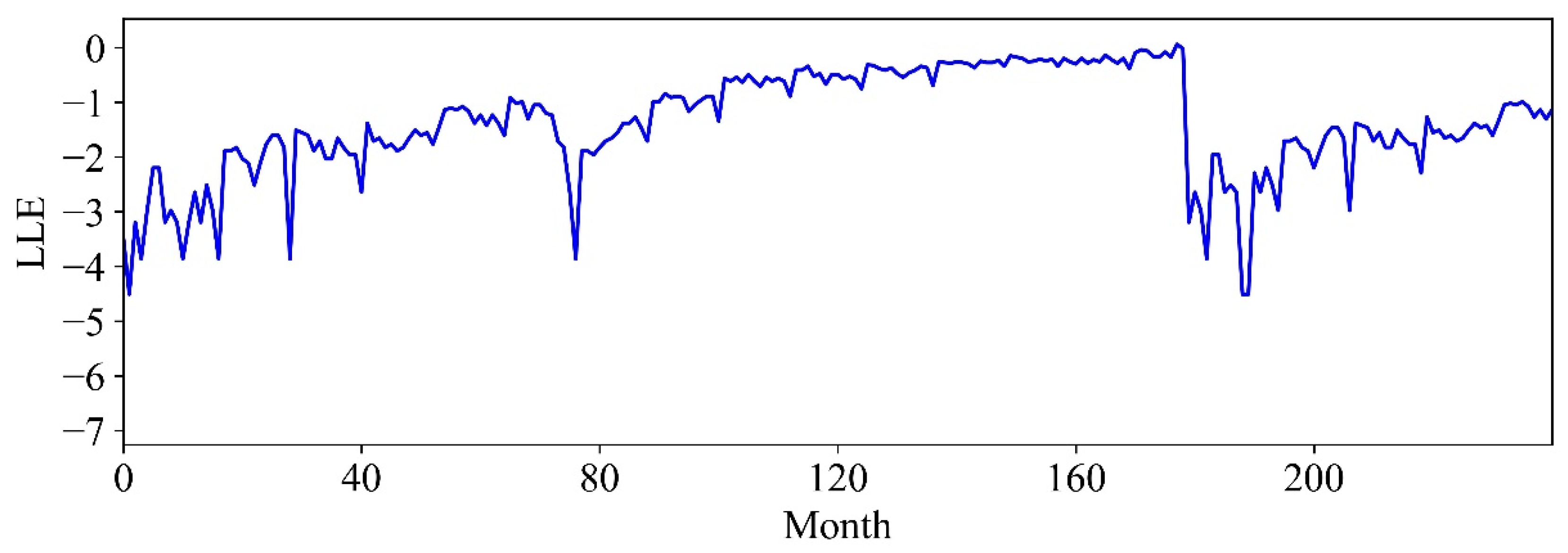
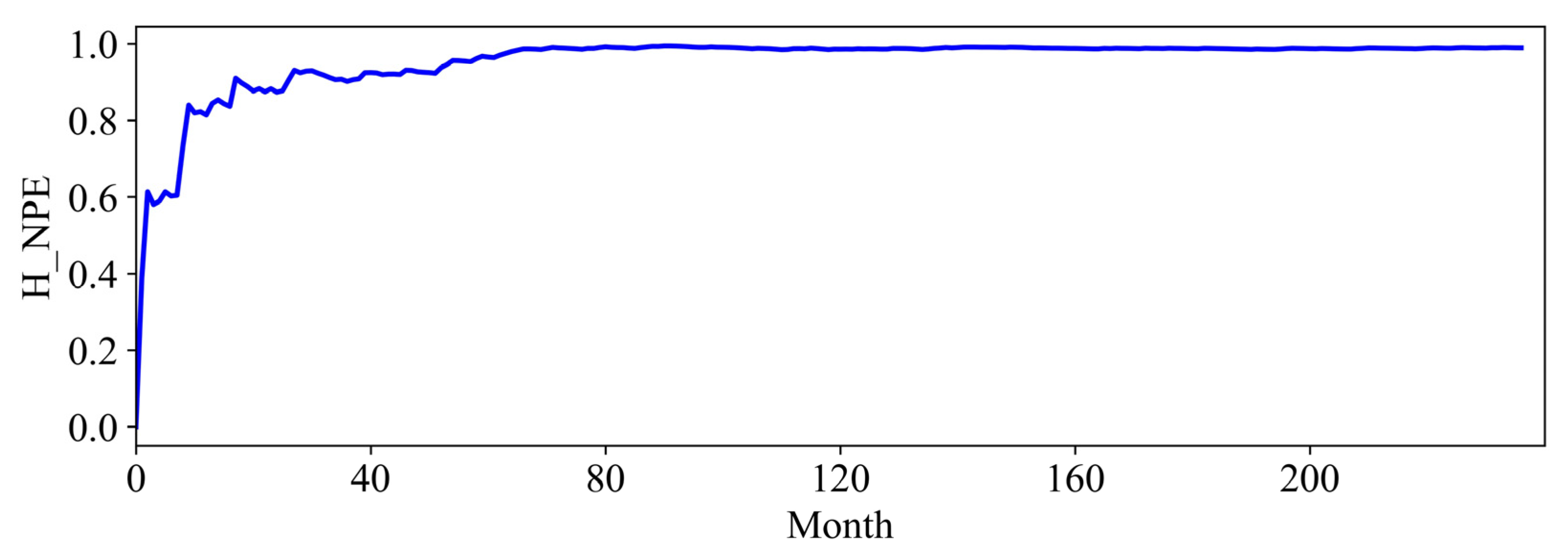
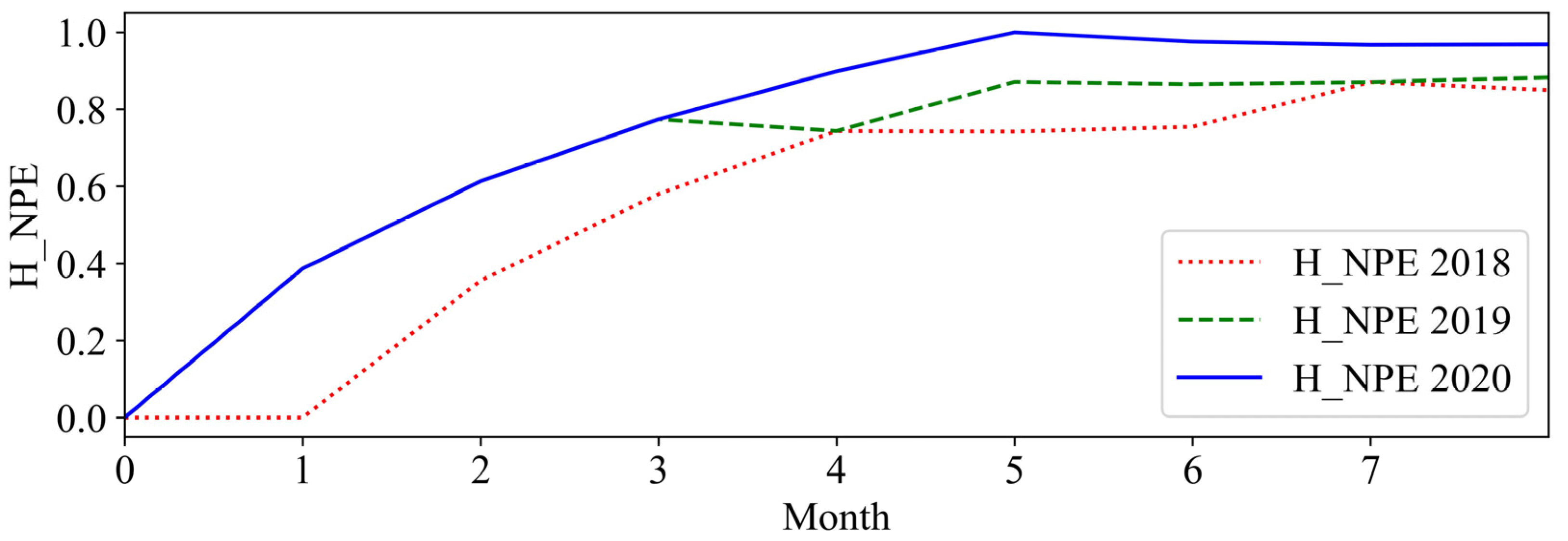
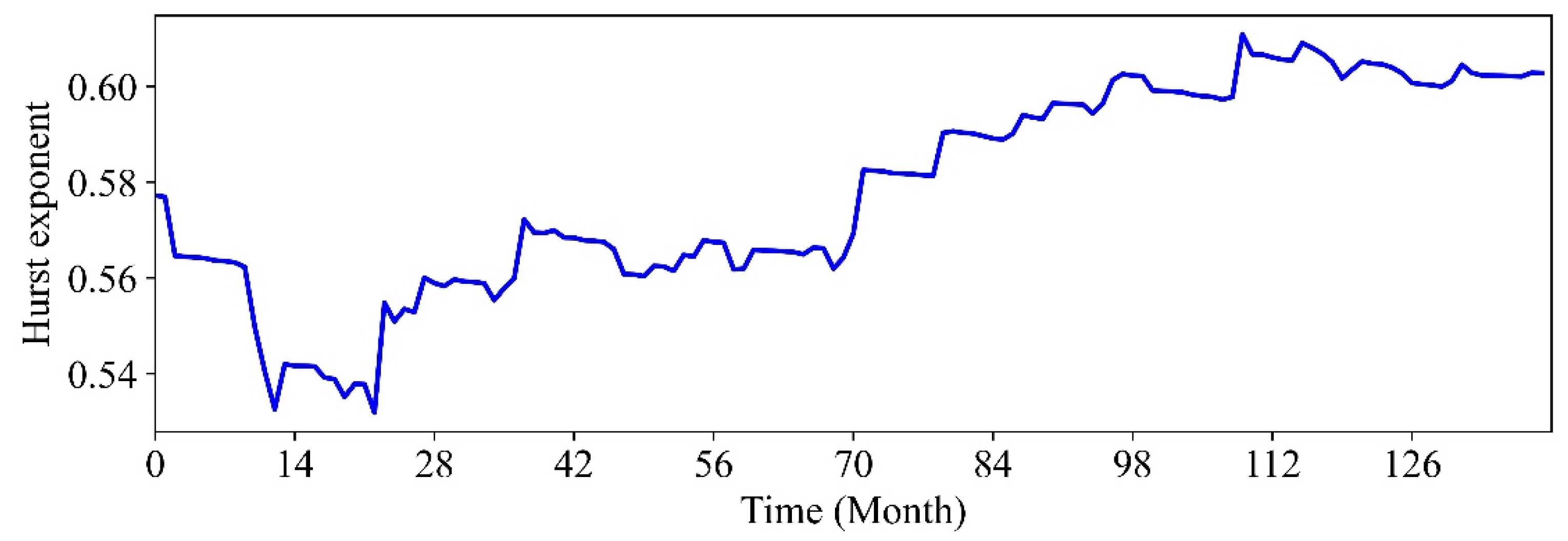
In this paper, comprehensive methods have been proposed for evaluating port resilience and throughput forecasting based on nonlinear time series analysis. The data analytics techniques can provide managerial insights for decision makers in understanding, characterizing, and predicting port productivity. First, the port resilience was evaluated using both nonlinear time-series analysis and statistical methods to help policymakers gain a deeper understanding of the resilience properties of maritime logistics in a disruptive market environment. In particular, the port throughput resilience against disruptions has been investigated through historical events such as the 2009 financial crisis and the COVID-19 pandemic. Nonlinear data analytics techniques for improving decision-making include Lyapunov exponents, entropy analysis, and Hurst exponents, which demonstrated the nonlinearity and chaotic tendency of a dynamic system.

Next, a robust forecasting method has been proposed by combining LSTM and RF to draw on the strengths of each strategy while avoiding their weaknesses. Then, the forecasting performance was extensively evaluated for the proposed hybrid method and a set of well-known algorithms, including RNN, LSTM, and RF. The performance evaluation metrics used were MSE, MAE, MAPE, RMSE, and RMSLE. Furthermore, the DM and HLN statistical significance tests were used to demonstrate the proposed empirical findings. All the evaluation results indicated that the proposed method outperformed all benchmarking models used in this study for both long- and short-term prediction. The proposed hybrid algorithm was the top-performing strategy across all measures at a 95% confidence level. The test results confirmed the superiority of the proposed hybrid method for throughput prediction against market volatility. In addition, the prediction results show that this study has many other possible applications in nonlinear time series forecasting and provides a new paradigm for the development of port productivity forecasting.

In more detail, this study makes major contributions to the theory and practice of both data analytics and dynamical behaviour for port productivity. As part of the first contribution, powerful analysis tools are proposed to investigate complex and nonlinear system behaviour, helping decision makers gain a better understanding of the dynamic behaviour of port productivity; the resilience mechanisms of port operations under external disturbances were explored by data analytics and statistical methods. In addition, a robust forecasting method has been proposed in this paper, which could be used to analyse complex maritime logistics patterns in the event of disruptions. This method employs a hybrid approach: first, an LSTM is applied to represent the temporal characteristics of a time series, followed by an RF for residuals from the model fitting. Therefore, port authorities can better prepare for future planning and operations based on the results obtained in the past through the proposed algorithm. Furthermore, the third contribution is that this study provides new insights into the mechanisms for clarifying system dynamic behaviour via nonlinear time series theory, such as in economic and financial forecasting problems.

In this study, the forecasting method was based on univariate analysis for training on the historical data. However, the expansion of multiple input variables, such as storage capacity of the terminal yard, ship turnaround time, container dwell time, berth/crane productivity, custom declaration time, etc., will make the forecasting method more comprehensive through learning various relationships that affect port productivity. For further studies, nonlinear control techniques could be used to help port authorities make systemic decisions that improve productivity and profitability.

References

1. Justice, V.; Bhaskar, P.; Pateman, H.; Cain, P.; Cahoon, S. US container port resilience in a complex and dynamic world. Marit. Policy Manag. 2016, 43, 179–191. [Google Scholar] [CrossRef]
2. Lam, J.S.; Notteboom, T. The greening of ports: A comparison of port management tools used by leading ports in Asia and Europe. Transp. Rev. 2014, 34, 169–189. [Google Scholar] [CrossRef]
3. Milenković, M.; Milosavljevic, N.; Val, S. Container flow forecasting through neural networks based on metaheuristics. Operational Res. 2021, 21, 965–997. [Google Scholar]
4. Frantzeskaki, N.; Wittmayer, J.; Loorbach, D. The role of partnerships in ‘realising’ urban sustainability in Rotterdam’s City Ports Area, The Netherlands. J. Clean. Prod. 2014, 65, 406–417. [Google Scholar] [CrossRef]
5. Kim, S.; Chiang, B.G. The role of sustainability practices in international port operations: An analysis of moderation effect. J. Korea Trade 2017, 21, 125–144. [Google Scholar] [CrossRef]
6. Marchese, D.; Reynolds, E.; Bates, M.E.; Morgan, H.; Clark, S.S.; Linkov, I. Resilience and sustainability: Similarities and differences in environmental management applications. Sci. Total Environ. 2018, 613, 1275–1283. [Google Scholar] [CrossRef]
7. Mubarik, M.S.; Naghavi, N.; Mubarik, M.; Kusi-Sarpong, S.; Khan, S.A.; Zaman, S.I.; Kazmi, S.H. Resilience and cleaner production in industry 4.0: Role of supply chain mapping and visibility. J. Clean. Prod. 2021, 292, 126058. [Google Scholar] [CrossRef]
8. Tsai, F.M.; Huang, L.J. Using artificial neural networks to predict container flows between the major ports of Asia. Int. J. Prod. Res. 2017, 55, 5001–5010. [Google Scholar] [CrossRef]
9. Holling, C.S. Resilience and stability of ecological systems. Annu. Rev. Ecol. Syst. 1973, 4, 1–23. [Google Scholar] [CrossRef] [Green Version]
10. Timmerman, P. Vulnerability, resilience and the collapse of society. In A Review of Models and Possible Climatic Applications; Institute for Environmental Studies, University of Toronto: Toronto, ON, Canada, 1981. [Google Scholar]
11. Westman, W.E. Resilience: Concepts and measures. In Resilience in Mediterranean-Type Ecosystems; Springer: Dordrecht, The Netherlands, 1986; pp. 5–19. [Google Scholar]
12. Tang, O.; Musa, S.N. Identifying risk issues and research advancements in supply chain risk management. Int. J. Prod. Econ. 2011, 133, 25–34. [Google Scholar] [CrossRef] [Green Version]
13. Chen, H.; Cullinane, K.; Liu, N. Developing a model for measuring the resilience of a port-hinterland container transportation network. Transp. Res. Part E Logist. Transp. Rev. 2017, 97, 282–301. [Google Scholar] [CrossRef]
14. Shaw, D.R.; Grainger, A.; Achuthan, K. Multi-level port resilience planning in the UK: How can information sharing be made easier? Technol. Forecast. Soc. Chang. 2017, 121, 126–138. [Google Scholar] [CrossRef]
15. Sazvar, Z.; Tafakkori, K.; Oladzad, N.; Nayeri, S. A capacity planning approach for sustainable-resilient supply chain network design under uncertainty: A case study of vaccine supply chain. Comput. Ind. Eng. 2021, 159, 107406. [Google Scholar] [CrossRef]
16. Lee, H.; Aldwin, C.M.; Kang, S.; Ku, X. Vulnerability and resilience among older South Korean Vietnam war veterans: A latent profile analysis. Psychol. Serv. 2022, 19, 95. [Google Scholar] [CrossRef] [PubMed]
17. Cuong, T.N.; Kim, H.S.; Xu, X.; You, S.S. Container throughput analysis and seaport operations management using nonlinear control synthesis. Appl. Math. Model. 2021, 100, 320–341. [Google Scholar] [CrossRef]
18. Wang, C.N.; Nguyen, N.A.; Fu, H.P.; Hsu, H.P.; Dang, T.T. Efficiency assessment of seaport terminal operators using DEA Malmquist and epsilon-based measure models. Axioms 2021, 10, 48. [Google Scholar] [CrossRef]
19. Xie, G.; Zhang, N.; Wang, S. Data characteristic analysis and model selection for container throughput forecasting within a decomposition-ensemble methodology. Transp. Res. Part E Logist. Transp. Rev. 2017, 108, 160–178. [Google Scholar] [CrossRef]
20. Saini, S.; Roy, D.; de Koster, R. A stochastic model for the throughput analysis of passing dual yard cranes. Comput. Oper. Res. 2017, 87, 40–51. [Google Scholar] [CrossRef]
21. Gosasang, V.; Chandraprakaikul, W.; Kiattisin, S. A comparison of traditional and neural networks forecasting techniques for container throughput at Bangkok port. Asian J. Shipp. Logist. 2011, 27, 463–482. [Google Scholar] [CrossRef] [Green Version]
22. Alshboul, O.; Almasabha, G.; Shehadeh, A.; Al Hattamleh, O.; Almuflih, A.S. Optimization of the Structural Performance of Buried Reinforced Concrete Pipelines in Cohesionless Soils. Materials 2022, 15, 4051. [Google Scholar] [CrossRef] [PubMed]
23. Liu, Y.; Chen, Y. Application of grey system model in throughput forecasting of inland river port. Port Waterw. Eng. 2006, 4, 31–34. [Google Scholar]
24. Shankar, S.; Ilavarasan, P.V.; Punia, S.; Singh, S.P. Forecasting container throughput with long short-term memory networks. Ind. Manag. Data Syst. 2020, 120, 425–441. [Google Scholar] [CrossRef]
25. Yang, C.H.; Chang, P.Y. Forecasting the demand for container throughput using a mixed-precision neural architecture based on CNN–LSTM. Mathematics 2020, 8, 1784. [Google Scholar] [CrossRef]
26. Shankar, S.; Punia, S.; Ilavarasan, P.V. Deep learning-based container throughput forecasting: A triple bottom line approach. Ind. Manag. Data Syst. 2021, 121, 2100–2117. [Google Scholar] [CrossRef]
27. Punia, S.; Nikolopoulos, K.; Singh, S.P.; Madaan, J.K.; Litsiou, K. Deep learning with long short-term memory networks and random forests for demand forecasting in multi-channel retail. Int. J. Prod. Res. 2020, 58, 4964–4979. [Google Scholar] [CrossRef]
28. Lin, W.; Wu, Z.; Lin, L.; Wen, A.; Li, J. An ensemble random forest algorithm for insurance big data analysis. IEEE Access 2017, 5, 16568–16575. [Google Scholar] [CrossRef]
29. Fischer, T.; Krauss, C. Deep learning with long short-term memory networks for financial market predictions. Eur. J. Oper. Res. 2018, 270, 654–669. [Google Scholar] [CrossRef] [Green Version]
30. Johannesen, N.J.; Kolhe, M.; Goodwin, M. Relative evaluation of regression tools for urban area electrical energy demand forecasting. J. Clean. Prod. 2019, 218, 555–564. [Google Scholar] [CrossRef]
31. Islam, S.; Amin, S.H. Prediction of probable backorder scenarios in the supply chain using Distributed Random Forest and Gradient Boosting Machine learning techniques. J. Big Data 2020, 7, 1–22. [Google Scholar] [CrossRef]
32. Sipper, M.; Moore, J.H. Conservation machine learning: A case study of random forests. Sci. Rep. 2021, 11, 3629. [Google Scholar] [CrossRef] [PubMed]
33. Becker, A.; Caldwell, M.R. Stakeholder perceptions of seaport resilience strategies: A case study of Gulfport (Mississippi) and Providence (Rhode Island). Coast. Manag. 2015, 43, 1–34. [Google Scholar] [CrossRef] [Green Version]
34. Omer, M.; Mostashari, A.; Nilchiani, R.; Mansouri, M. A framework for assessing resiliency of maritime transportation systems. Marit. Policy Manag. 2012, 39, 685–703. [Google Scholar] [CrossRef]
35. Lhomme, S. Vulnerability and resilience of ports and maritime networks to cascading failures and targeted attacks. In Maritime Networks; Routledge: London, UK, 2015; pp. 253–265. [Google Scholar]
36. Nazemzadeh, M.; Vanelslander, T. The container transport system: Selection criteria and business attractiveness for North-European ports. Marit. Econ. Logist. 2015, 17, 221–245. [Google Scholar] [CrossRef]
37. Trepte, K.; Rice, J.B., Jr. An initial exploration of port capacity bottlenecks in the USA port system and the implications on resilience. Int. J. Shipp. Transp. Logist. 2014, 6, 339–355. [Google Scholar] [CrossRef] [Green Version]
38. Verschuur, J.; Koks, E.E.; Hall, J.W. Port disruptions due to natural disasters: Insights into port and logistics resilience. Transp. Res. Part D Transp. Environ. 2020, 85, 102393. [Google Scholar] [CrossRef]
39. Notteboom, T.; Pallis, T.; Rodrigue, J.P. Disruptions and resilience in global container shipping and ports: The COVID-19 pandemic versus the 2008–2009 financial crisis. Marit. Econ. Logist. 2021, 23, 179–210. [Google Scholar] [CrossRef]
40. Sarkar, B.D.; Shankar, R.; Kar, A.K. A scenario-based interval-input output model to analyze the risk of COVID-19 pandemic in port logistics. J. Model. Manag. 2021; ahead-of-print. [Google Scholar] [CrossRef]
41. Marasco, A.; Romano, A. Inter-port interactions in the Le Havre-Hamburg range: A scenario analysis using a nonautonomous Lotka Volterra model. J. Transp. Geogr. 2018, 69, 207–220. [Google Scholar] [CrossRef]
42. Zhang, W.; Lam, J.S. An empirical analysis of maritime cluster evolution from the port development perspective–Cases of London and Hong Kong. Transp. Res. Part A Policy Pract. 2017, 105, 219–232. [Google Scholar] [CrossRef]
43. Slotine, J.J.; Li, W. Applied Nonlinear Control; Prentice Hall: Englewood Cliffs, NJ, USA, 1991. [Google Scholar]
44. Morris, S.A.; Pratt, D. Analysis of the Lotka–Volterra competition equations as a technological substitution model. Technol. Forecast. Soc. Chang. 2003, 70, 103–133. [Google Scholar] [CrossRef]
45. Alshboul, O.; Shehadeh, A.; Tatari, O.; Almasabha, G.; Saleh, E. Multiobjective and multivariable optimization for earthmoving equipment. J. Facil. Manag. 2022; ahead-of-print. [Google Scholar] [CrossRef]
46. Schulze, P.M.; Prinz, A. Forecasting container transshipment in Germany. Appl. Econ. 2009, 41, 2809–2815. [Google Scholar] [CrossRef]
47. Niu, M.; Hu, Y.; Sun, S.; Liu, Y. A novel hybrid decomposition-ensemble model based on VMD and HGWO for container throughput forecasting. Appl. Math. Model. 2018, 57, 163–178. [Google Scholar] [CrossRef]
48. Chen, S.H.; Chen, J.N. Forecasting container throughputs at ports using genetic programming. Expert Syst. Appl. 2010, 37, 2054–2058. [Google Scholar] [CrossRef]
49. Ma, X.; Yu, Q.; Liu, J. Modeling Urban Freeway Rear-End Collision Risk Using Machine Learning Algorithms. Sustainability 2022, 14, 12047. [Google Scholar] [CrossRef]
50. Liu, Z.; Lei, H.; Lei, L.; Sheng, H. Spatial Prediction of Total Nitrogen in Soil Surface Layer Based on Machine Learning. Sustainability 2022, 14, 11998. [Google Scholar] [CrossRef]
51. Graves, A.; Mohamed, A.R.; Hinton, G. Speech recognition with deep recurrent neural networks. In Proceedings of the 2013 IEEE International Conference on Acoustics, Speech and Signal Processing, Vancouver, BC, Canada, 26–30 May 2013; pp. 6645–6649. [Google Scholar]
52. Al Shehri, W.; Almalki, J.; Mehmood, R.; Alsaif, K.; Alshahrani, S.M.; Jannah, N.; Alangari, S. A Novel COVID-19 Detection Technique Using Deep Learning Based Approaches. Sustainability 2022, 14, 12222. [Google Scholar] [CrossRef]
53. Pawar, P.; Ainapure, B.; Rashid, M.; Ahmad, N.; Alotaibi, A.; Alshamrani, S.S. Deep Learning Approach for the Detection of Noise Type in Ancient Images. Sustainability 2022, 14, 11786. [Google Scholar] [CrossRef]
54. Ferreira, K.J.; Lee, B.H.; Simchi-Levi, D. Analytics for an online retailer: Demand forecasting and price optimization. Manuf. Serv. Oper. Manag. 2016, 18, 69–88. [Google Scholar] [CrossRef] [Green Version]
55. Mejia, J.; Avelar-Sosa, L.; Mederos, B.; Ramírez, E.S.; Roman, J.D. Prediction of time series using an analysis filter bank of LSTM units. Comput. Ind. Eng. 2021, 157, 107371. [Google Scholar] [CrossRef]
56. Baird, A. Analysis of private seaport development: The port of Felixstowe. Transport Policy. 1999, 6, 109–122. [Google Scholar] [CrossRef]
57. Ye, Y.; Zhang, Y.; Wang, Q.; Wang, Z.; Teng, Z.; Zhang, H. Fault diagnosis of high-speed train suspension systems using multiscale permutation entropy and linear local tangent space alignment. Mech. Syst. Signal Process. 2020, 138, 106565. [Google Scholar] [CrossRef]
58. Ng, A.K.; Liu, J.J. The port and maritime industries in the post-2008 world: Challenges and opportunities. Res. Transp. Econ. 2010, 27, 1–3. [Google Scholar] [CrossRef]
59. Fusillo, M.; Haralambides, H. Do carrier expectations indicate industry structure in container shipping? An econometric analysis. J. Shipp. Trade 2020, 5, 1–6. [Google Scholar] [CrossRef]
60. Sohn, J.I.; Alakshendra, A.; Kim, H.J.; Kim, K.H.; Kim, H.D. Understanding the New Characteristics and Development Strategies of Coastal Tourism for Post-COVID-19: A Case Study in Korea. Sustainability 2021, 13, 7408. [Google Scholar] [CrossRef]
61. Hwarng, H.B.; Xie, N. Understanding supply chain dynamics: A chaos perspective. Eur. J. Oper. Res. 2008, 184, 1163–1178. [Google Scholar] [CrossRef]
62. Wolf, A.; Swift, J.B.; Swinney, H.L.; Vastano, J.A. Determining Lyapunov exponents from a time series. Phys. D Nonlinear Phenom. 1985, 16, 285–317. [Google Scholar] [CrossRef] [Green Version]
63. Clément, A.; Laurens, S. An alternative to the Lyapunov exponent as a damage sensitive feature. Smart Mater. Struct. 2011, 20, 025017. [Google Scholar] [CrossRef] [Green Version]
64. Jahanshahi, H.; Yousefpour, A.; Wei, Z.; Alcaraz, R.; Bekiros, S. A financial hyperchaotic system with coexisting attractors: Dynamic investigation, entropy analysis, control and synchronization. Chaos Solitons Fractals 2019, 126, 66–77. [Google Scholar] [CrossRef]
65. Bandt, C.; Pompe, B. Permutation entropy: A natural complexity measure for time series. Phys. Rev. Lett. 2002, 88, 174102. [Google Scholar] [CrossRef]
66. Corazza, M.; Malliaris, A.T. Multi-fractality in foreign currency markets. Multinatl. Financ. J. 2002, 6, 65–98. [Google Scholar] [CrossRef]
67. Tzouras, S.; Anagnostopoulos, C.; McCoy, E. Financial time series modeling using the Hurst exponent. Phys. A Stat. Mech. Its Appl. 2015, 425, 50–68. [Google Scholar] [CrossRef]
68. Hurst, H.E. Long-term storage capacity of reservoirs. Trans. Am. Soc. Civ. Eng. 1951, 116, 770–799. [Google Scholar] [CrossRef]
69. Harvey, D.; Leybourne, S.; Newbold, P. Testing the equality of prediction mean squared errors. Int. J. Forecast. 1997, 13, 281–291. [Google Scholar] [CrossRef]
70. Alshboul, O.; Shehadeh, A.; Mamlook, R.E.; Almasabha, G.; Almuflih, A.S.; Alghamdi, S.Y. Prediction Liquidated Damages via Ensemble Machine Learning Model: Towards Sustainable Highway Construction Projects. Sustainability 2022, 14, 9303. [Google Scholar] [CrossRef]
71. Xie, W.; Zhuge, S.; Wu, Y.; Xiao, D. Simulation-Based Operational Evaluation of a Single-Berth Multipurpose Seaport with Wharf Space Restriction. J. Mar. Sci. Eng. 2021, 9, 883. [Google Scholar] [CrossRef]
72. Wu, X.; Gao, Y.; Jiao, D. Multi-label classification based on random forest algorithm for non-intrusive load monitoring system. Processes 2019, 7, 337. [Google Scholar] [CrossRef] [Green Version]
73. Dietterich, T.G. An experimental comparison of three methods for constructing ensembles of decision trees: Bagging, boosting and randomization. Mach. Learn. 1998, 32, 139–157. [Google Scholar]
74. Chen, H.; Wan, Q.; Wang, Y. Refined Diebold-Mariano test methods for the evaluation of wind power forecasting models. Energies 2014, 7, 4185–4198. [Google Scholar] [CrossRef]
75. Diebold, F.; Mariano, R. Comparing predictive accuracy. J. Bus. Econ. Stat. 1995, 13, 253–265. [Google Scholar]
Figure 1. The shares in container throughput by Korean ports in 2020. Unit: TEU, %. Source: authors’ compilation adapted from 2020 container statistics of Busan port.
Sustainability 14 13985 g001
Figure 2. Container throughput of Busan port by month, January 2001 to December 2020. Source: authors’ compilation adapted from 2020 container statistics of Busan Port.
Sustainability 14 13985 g002
Figure 3. Busan port’s monthly throughput for the past three years (2018–2020). Source: authors’ compilation adapted from 2020 container statistics of Busan port.
Sustainability 14 13985 g003
Figure 4. The historical monthly returns of container throughput (Busan port).
Sustainability 14 13985 g004
Figure 5. Empirical distribution of monthly returns in the time period 2001–2020.
Sustainability 14 13985 g005
Figure 6. Lyapunov exponent spectrum of port throughput (Busan port).
Sustainability 14 13985 g006
Figure 7. Temporal variation in permutation entropy of Busan port throughput.
Sustainability 14 13985 g007
Figure 8. Entropy comparison of Busan port in the period 2018–2020.
Sustainability 14 13985 g008
Figure 9. Hurst exponent over a sliding window of 140 observations (from May 2009 to December 2020).
Sustainability 14 13985 g009
Figure 10. Structures of the deep learning method. (a) RNN and (b) LSTM.
Sustainability 14 13985 g010aSustainability 14 13985 g010b
Figure 11. Structure and workings of the random forest algorithm (RF).
Sustainability 14 13985 g011
Figure 12. Forecasting performance for deep learning models in time series data: (a) RNN, (b) LSTM, (c) RF, and (d) LSTM-RF (hybrid method) (unit: million TEUs).
Sustainability 14 13985 g012aSustainability 14 13985 g012b
Figure 13. The residual errors from forecasts on time series.
Sustainability 14 13985 g013