Shadow Economy Estimation Using Cash Demand Approach: The Case of Serbia

Abstract

Informalities in the Serbian economy seem to be relatively persistent and widespread, as suggested by some empirical evidence and numerous anecdotal evidence provided by citizens and companies. Nevertheless, the shadow—or informal—economy is a rather complicated phenomenon with a complex set of causes and consequences, implying that there are no universally accepted definitions nor quantification methods for determining the relative size of its impact. This paper takes a pioneering approach using the “monetary method” or the “currency demand approach” for the Serbian economy, based on econometric estimates of the demand for money. In this context, we rely on the well-known currency demand approach, expanding and applying it to the case of Serbia. Against the backdrop of the key research question, we found that the shadow economy in Serbia has decreased to roughly 20% of GDP in late 2021 from roughly 30% in 2005.

1. Introduction

The informal or shadow economy, although often imprecisely defined, represents a major socio-economic challenge across the world, particularly severe in developing countries. The informal economy refers to two components: (a) all economic activities undertaken by workers and economic units are not covered or are not sufficiently covered by formal arrangements in regard to the law or in practice, and (b) it does not take into account illicit activities [1]. One of the definitions of the shadow economy is that it is a set of all market and legal production and service activities that are hidden by a conscious effort from government authorities for a number of the following reasons: to avoid income tax collection, value-added tax, or tax on some other basis; to avoid paying social security contributions; to avoid certain requirements arising from labor legislation such as minimum wages, maximum working hours, safety standards; and to avoid certain administrative procedures [2].

Significantly, although tax evasion is one of the main macroeconomic factors behind the emergence of the shadow economy, the erosion of budget revenues constitutes a relatively more harmful consequence. This reduces the fiscal room, thus limiting the financing of various public services [3], which is reflected in the deepening of the budget deficit. Additionally, unregistered businesses represent unfair competition to legally legitimate companies, especially in terms of reporting and tax liabilities payments [4].

In order to mitigate the aforementioned effects of tax evasion and the erosion of budget revenues throughout the shadow economy, it is necessary to understand their causes and the effects of public policy measures aimed at curtailing them. Accordingly, the quantification of a shadow economy should be prioritized. However, its measuring is challenging as it is difficult to directly assess a phenomenon that individuals or institutions deliberately keep hidden, such as tax evasion [5], etc.

This paper contextualises this issue in the case of Serbia—a middle-income European country with a PPP GDP per capita of only about 40% of the 2021 EU average and with an institutional, political, and economic legacy inducing a prominent inclination towards shadow economic activity.

Indeed, in the aftermath of Yugoslavia’s collapse in the 1990s, the Serbian economy faced a very deep political crisis and international sanctions—provoking severe, profound, and long-lasting institutional deterioration. Following the decade characterised by a fall in income, a rise in poverty, and hyperinflation [6], Serbia’s belated transition to a market economy began as late as the early 2000s. However, the ensuing episode of strong growth and political stability was abruptly stopped by the effects of the 2008 global economic crisis—implying that Serbia’s economy never managed to fully catch up with its Central and East European neighbors.

Against this historical backdrop, Serbia’s shadow economy flourished in all forms, seemingly having reached about 50% of GDP by the end of the 1990s [7]. Significant efforts in reforming taxation and various elements of the business environment were made since the end of the 1990s, which contributed to a subsequent decrease in the shadow economy—resulting in improved tax inflows—albeit it remains relatively widespread.

This paper aims to complement the quantification of the shadow economy in Serbia so far and thus contribute to appropriate monitoring efforts and quality public policies aimed towards addressing its consequences. By doing so, the key research question is: what is the level of the shadow economy in Serbia, and what was its trend between 2005 and 2021?

There have been a few attempts so far to quantify the shadow economy in Serbia [8]. As the measurement of something intentionally hidden represents a challenge per se, each of these studies expectedly contains some methodological limitations. Most of the measurements are partial in terms of their coverage of different dominant forms of the shadow economy. Some of them are also based on relatively arbitrary and/or perception-based methods, such as surveys or polls, which are both expensive and difficult to properly organise. Most of them are ad hoc and therefore are published in irregular frequencies, and in the case of some methods, even produced only once. Given the different methods used, the results obtained are incomparable.

In light of these observations and setbacks, our paper aims to provide a novel, more comprehensive, and more affordable approach which can be used to frequently quantify the presence of the shadow economy in Serbia as well as to monitor its trends.

We rely on the Currency Demand Approach (CDA) that first empirically estimates the level of currency in circulation using its main theoretically derived determinants such as the level of income, the interest rate—as the opportunity cost of holding cash—and a variable measuring tax burden or other incentives for informal transactions. Subsequently, the excess currency in circulation is assessed as the difference between the estimated level of currency in circulation and the level obtained by the same equation but with setting the incentive variable to the level at which all transactions in the economy would be registered (external to the shadow economy). Finally, the unregistered income is assessed using the obtained level of excess currency and the money velocity.

Although this method has been applied extensively, covering a wide range of countries—including the OECD members and many developing countries—it has never been used for the Serbian case. This indicator relies on publicly available historical data—which allows for the construction of a time series from the year 2005 to 2021. This is the first attempt at making an integral overview of the dynamics of the shadow economy in Serbia.

Finally, our estimation is well grounded in similar studies conducted internationally. More significantly, it is well adapted to the specific context of Serbia in terms of period coverage as well as the choice and design of variables to reflect the theoretically proposed definitions in the empirical model. According to a report by NALED [9], aversion to tax payments remains the main motive behind the shadow economy in Serbia. Considering this finding, and in order to accurately capture the relevant changes in the most notable tax regimes, we also develop an original means of designing the variable measuring tax burden, crucial to the process of quantifying the shadow economy.

Thus, we propose a rather objective and relatively affordable indicator of the shadow economy for Serbia, which can be produced in annual, quarterly, or possibly even shorter frequencies—providing valuable and timely information for policy monitoring, evaluation, and a more informed policy formulation.

In this publication, we measure the level and trend of the shadow economy. Our indicator reports that the shadow economy has been in a downward trend since the early 2000s, decreasing by a total of some 10pp to approx. 20% in the early 2020s. Nevertheless, the indicator reports two reversal episodes within this period—in the aftermath of the 2008 global financial crisis, i.e., in the early 2010s, and the other in the aftermath of the COVID-19 pandemic. However, it seems that even despite these reversal episodes, the shadow economy has continued to decrease as early as 2021.

Section 2 presents the existing literature on the currency demand approach while nesting it in the broader taxonomy of applied approaches in the estimation of the shadow economy. In the same section, we show the results of the existing estimation of the shadow economy in Serbia. Section 3 presents our estimation model, data, and variables. Section 4 presents the results and discussion, and Section 5 contains concluding remarks.

2. Overview of the Relevant Literature

Our study aims to complement the efforts in assessing the size of the shadow economy in Serbia.

Shadow economy, as defined in our introductory section following the major strand of literature [2,3], is a broadly studied phenomenon across the world. A wide interest in the shadow economy started back in the 1980s and still represents a live field of research. It is driven by the government’s need to understand the real volume of the GDP, well documented, for example, by Schneider and Enste [4] and Alm [5] for tax evasion. The main questions in the literature seem to be related to the causes of the shadow economy and its measurement. Arsić et al. [10] produced a comprehensive overview of the studies on the causes of the shadow economy, while Alm [5] provided a discussion on the causes of tax evasion—this being a relatively tightly related phenomenon.

As our study aims to complement the efforts in assessing the size of the shadow economy in Serbia, we first present the results of the existing studies by classifying them according to the applied methodological approach (Section 2.1). Then we present a literature overview while providing the theoretical and empirical background of the best-known and most widely used approaches in the quantification of the shadow economy (Section 2.2).

2.1. Available Estimates of the Shadow Economy in Serbia

The available approaches in the literature to measure informality can be classified into three categories: (1) direct methods, (2) indirect methods, and (3) MIMIC or model approaches [11].

(1)

Direct Methods

Direct methods include (a) inspection visits—where the assessment of the macro-level hidden economy needs to rely on random audit, and (b) different kinds of public or private surveys where respondents are asked to report on known hidden economic activities. The survey method was applied in Serbia two consecutive times [12]. It sought to measure the perception of registered entities about the unregistered activities of their competitors. 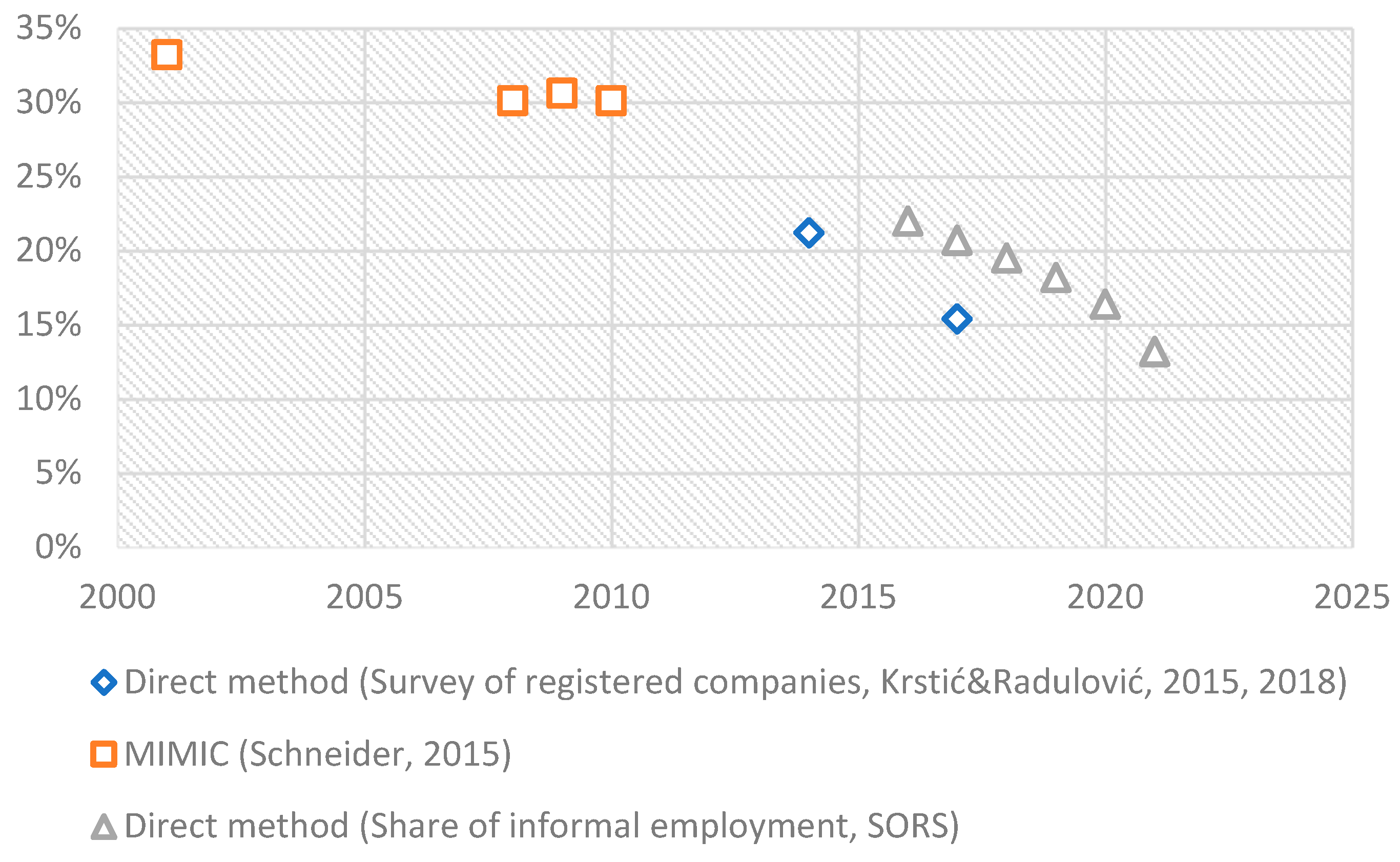This method was applied in Serbia for the last time in 2017 [8]. At that time, the volume of the shadow economy was measured at the level of 15.4% of GDP, significantly lower than in 2012, when it was measured at 21.2% of GDP using the same method. In 2017, an innovative survey method was also applied to gather data on undeclared salaries and company profits. The results indicated approximately the same volume of the shadow economy, 14.9% of GDP, as based on the application of the (old) survey method targeting undeclared income. The survey was conducted during September and October of 2017 with a sample including 1049 business entities, i.e., 540 companies and 509 entrepreneurs. Most of the respondents were business owners or managers. The authors underlined in their conclusions that this estimate represented the lower limit of the shadow economies scope since the research included only registered companies and entrepreneurs.

Compared to other countries where the innovative survey method has been applied, the estimated shadow economy in Serbia (14.9% of GDP) is lower than in Montenegro (24.5%) and Latvia (20.3%), while it is on the same approximate level as registered in Estonia (15.4%) and Lithuania (16.5%). However, the share of unregistered companies, which are not included in this assessment, is significantly higher in Serbia compared to the Baltic countries. According to business estimates, 17.2% of companies in their business industry were perceived as not registered.

The same report showed that in Serbia, it is informal employment, i.e., the partial or full payment of wages in cash, that comprises a significantly larger portion of the shadow economy than the undeclared business surplus (profit). Out of 100 dinars in the shadow economy, approximately 62 dinars are considered as payment of undeclared salaries of employees and 38 dinars as undeclared profits.

Although our approach provides direct insight into the structure of different forms of the shadow economy, the method nonetheless carries limitations. One such finding showed that the dominant aspect of the shadow economy underreports labor costs of companies that pay workers’ salaries in cash. Namely, the subjective nature and relatively narrow focus are reflected in the fact that this approach offers a rather lower-bound estimate of the shadow economy. Moreover, it is a relatively expensive method that is not usually measured on a regular basis which would not allow for a timely signal to policymakers of the trends in the shadow economy and its possible reversals.

Another available direct method applied in Serbia since 2014 is the measure of informal employment through the Labor Force Survey, which is conducted on a quarterly basis by the Statistical Office of the Republic of Serbia following the internationally aligned methodology by the International Labour Organization. According to this survey, persons who are informally employed are employed workers without a written employment contract, self-employed persons in unregistered business entities, as well as assisting family members. The estimated share of informally employed in the total employed population was 22% in 2016 (including workers in agriculture), decreasing to 13.2% in 2021 (Figure 1).

(2)

Indirect Methods

These methods are implemented by the use of discrepancies found in official records (such as disparities between official and actual labour force in the economy, disparities between consumption and national income, different monetary methods, etc.) as proxies for the size of the informal sector. Indirect methods use the discrepancy between the estimated actual economic activity and the officially registered activity based on macroeconomic data as a proxy for the shadow economy. Their disadvantages in relation to direct methods are, firstly, that they cannot describe the structure of the shadow economy in such detail and, secondly, that they are not able to measure a precisely defined shadow economy. Therefore, it is considered that indirect methods provide an indicator of the upper limit of the shadow economy, while direct methods measure the lower limit of the shadow economy. The advantage of the indirect method is that it is often the more objective approach, considering all the shortcomings inherent to the survey (direct) methods, which are reflected in insincere answers and other difficulties related to the direct measurement of phenomena that are impermissible and undesirable. Some of the most commonly used indirect methods are: (a) the discrepancy between measured GDP by income and expenditure, (b) the discrepancy between formally registered labor and actual labor, (c) the method of comparing electricity consumption with reported income, and (e) a method based on estimating the need for cash in an economy and defining the shadow economy indicator by measuring the gap between cash in use and the estimated actual need for cash [13,14], which will be elaborated in more details as a theoretical basis for our study presented in the remainder of this paper.

Having completed a thorough investigation and, therefore, according to our present knowledge, this class of methods has not been applied to the Serbian context so far, and our attempt is a pioneering one.

(3)

MIMIC or Model Approach

While this approach may seem to belong to the indirect methodology, it diverges from the methods that were applied previously since it can create links between unobserved variables and observed indicators, making use of structural equations that model causal relationships amidst the unobserved variables. Utilising the MIMIC approach for the purpose of estimating the extent of the informal sector was initially introduced by Frey and Weck-Hanneman [15]. This method was used by Schneider et al. [10] to estimate the hidden economy in 11 Central and Eastern European countries, including Serbia, for the period from 2001 to 2010. To overcome the inherent drawback of the MIMIC approach, which is that it only gives relative estimated sizes of the extent of the shadow economy, and to obtain the absolute figures for the shadow economy, the authors used existing data from the currency demand approach applied to Hungary, Poland, and Slovenia, and for the other countries from Schneider [12] (having used the DYMIMIC method on 110 countries’ data to evaluate coefficients of main determinants of the shadow economy, while they used already available estimated level for some of the countries by other studies to calculate the absolute level of shadow economy) and Lackó [16] (having measured the shadow economy in transition countries using the physical input method—electricity).

The obtained estimate for the extent of the Serbian shadow economy was measured at 33.2% in 2001, declining to 30.1% in 2008, then increasing in 2009 to 30.6%, and decreasing again in 2010 to 30.1% (Figure 1). A minor increase in 2009 was perceivable for nearly all 11 countries. The results indicated that the extent of the shadow economy had decreased in Serbia over the period of economic growth and then remained near constant after the beginning of the economic crisis. Moreover, throughout the considered time frame (2000–2025), the extent of the shadow economy in Serbia is somewhat greater than the average values observed in the other 11 countries. Only in Bulgaria, the proportion of its shadow economy in percent of GDP relative to Serbia was greater (by 2.2 percentage points in 2010).

2.2. Currency Demand Approach: Relevant Theoretical Background and Practical Applications

The currency demand approach is usually classified among the indirect methods. The family of monetary methods traces its beginnings back to Cagan, Gutmann, and Feige [17,18,19]. This particular approach was popularised among economists by Tanzi [13]. Throughout the prior two decades, this approach has been widely used to estimate informality mainly in developed countries such as Tanzi [13] for the USA, Shima [20] for Norway, Klovland [21] for Norway and Sweden, Bovi and Castellucci [22] for Italy, and Bovi and Dell’Anno [23] for OECD countries. More recent studies cover developing countries such as Brambila and Cazzavilan for Mexico, Hernandez for Peru, Schneider and Bajada for Asia-Pacific countries, Koloane and Bodhlyera for South Africa, Dybka et al. for Poland, Dell’Anno and Davidescu for Romania, Ahumada et al. and Petranov et al. for Bulgaria, and Khan for Malaysia [24,25,26,27,28,29,30,31,32].

The primary assumption behind this kind of approach is that transactions in the informal sector mainly utilize cash to maintain their informal activities and to avoid any means of formalizing or recording their activities. Therefore, once we estimate the quantity of cash used for informal transactions, we should be able to estimate the size of the informal sector within the economy.

A general form of the Cagan [17] type demand function for currency can be expressed as follows:

$$C=A{\left(1+\Theta \right)}^{\alpha }{Y}^{\beta }{e}^{\gamma i}$$

(1)

where $C$ denotes cash balances, and $\Theta$ is a variable that induces agents to realize hidden transactions. This is a crucial variable that is featured in all currency models. It is based on the hypothesis that high taxes and government regulations are the main causes of shadow economic activities. Therefore, this incentive variable is usually estimated using GDP-normalized government consumption, tax rates (direct taxes, indirect taxes, etc.), or tax revenues to GDP. A higher $\Theta$ should have a positive influence on currency demand because agents will be more encouraged to address the informal sector, requiring more currency to fund transactions.

$Y$ represents a scale variable (for example, registered GDP). This variable is an approximation of the level of transactions within the economy. Surrogate measures can be GDP/consumption per capita. Lastly, $i$ quantifies the opportunity cost of holding cash (interest rate or inflation rate) and $A$ is a non-negative parameter. $Y$ should have a positive coefficient since a higher income stimulates a larger currency demand for transactions. Furthermore, $i$ should have a negative coefficient due to the increased opportunity cost of holding cash as the result of higher interest rates on deposits.

Estimating Equation (1) provides us with the estimated cash level in circulation $\tilde{C}$. The next step includes setting the incentive variable $\Theta$ to zero, as originally proposed by Tanzi [13] and used in many applications of the methodology. However, some relevant authors in more recent literature, such as Hernandez [25], Koloane and Bodhlyera [27], and Dybka et al. [28], have criticized the hypothesis of a zero tax rate as unrealistic for any economy and suggested using some version of a minimal tax rate for which there would be no tax evasion. To estimate the shadow economy, Dybka et al. [28] used the minimal recorded tax and social security contribution inflows. By applying the no-shadow-economy tax rate to the estimated model while keeping the coefficients of other variables constant, we find the estimated level of cash in circulation that would be needed if there was no (tax-related) incentive to perform operations within the shadow economy $\widehat{C}$. The difference between $\tilde{C}$ and $\widehat{C}$ allows for the estimation of extra currency ($EC$), i.e., the quantity of currency holdings that are caused by the incentive to avoid tax by operating in the unregistered economy. Put another way, the difference measures the quantity of unlawful money in the economy. In the second step, under the assumption that money velocity is the same in both formal and informal sectors, one can derive an estimate of the size of the informal economy by multiplying illegal money $EC$ (equals $\tilde{C}-\widehat{C}$) by money velocity ($v=Y/\left(M1\right)$).

Ahumada et al. [33] criticized the last assumption, which claims that money velocity is equal in the formal and informal sectors. They demonstrated that money velocity in the unofficial production is dependent on the income elasticity of cash demand. Thus, only when this elasticity equals one the assumption of the equal velocity of currency in the unofficial and official economy holds true. By the same token, in the case when this elasticity is not unitary, the authors propose the following correction that allows for the estimate of an amount of untaxed production, which represents a percentage of official GDP and is unbiased.

$$\frac{Y_H}{Y_R}={\left(\frac{C_H}{C_R}\right)}^{\frac{1}{\beta }}={\left(\frac{{\underset{\_}{Y}}_H}{{\underset{\_}{Y}}_R}\right)}^{\frac{1}{\beta }}$$

(2)

In Equation (2), $Y_H$ and $C_H$ stand for informal (hidden) income and excess cash (for hidden transactions), respectively, $Y_R$ and $C_R$ for registered income and cash for registered transactions, respectively, and $\frac{{\underset{\_}{Y}}_H}{{\underset{\_}{Y}}_R}$ is the “erroneous” ratio calculated under the restriction that $\beta =1$. Where $\beta$ represents the elasticity of cash demand to the level of income, which can be estimated from the currency demand function and is rarely equal to one.

3. Methodology, Data, and Variables

This paper departs from its key research question: what is the level of the shadow economy in Serbia, and what has been its trend in the past two decades?

More precisely, this study uses quarterly data series that cover a period from the 1st quarter of 2005 to the 3rd quarter of 2021. The choice of the period length of the study depended solely on data availability, that of the tax-related variable. The main sources of the data obtained for the study include the National Bank of Serbia, the Statistical Office of the Republic of Serbia, and the Ministry of Finance of the Government of Serbia.

3.1. Estimated Model

To capture the long-run relationships of the explanatory variables on currency demand, we considered the log version of Equation (1) throughout our analysis. Taking logs to both sides, the estimated equation of the demand for currency is given by the following equation:

$$C{R}_t={\alpha }_0+{\alpha }_1·Ta{x}_t+{\alpha }_2·GD{P}_t+{\alpha }_3·i_t+{\alpha }_4·C_t+{\epsilon }_t,$$

(3)

where:

$C{R}_t$	$\mathrm{is}$ registered cash in circulation in real terms at time t in national currency (dinar)
$GD{P}_t$	is natural logarithm of real GDP in national currency in the period t
$Ta{x}_t$	$\mathrm{is} \mathrm{natural} \mathrm{logarithm} \mathrm{of} \left(1+Tax Rate\right)$$(\mathrm{see} \mathrm{subsection} \mathrm{on} \mathrm{choice} \mathrm{of} TaxRate$ variable)
$i_t$	is average nominal interest rate for newly contracted deposits in local currency in the period t
$C_t$	is a dummy variable taking a value of 1 for the period covering the COVID-19 pandemic and 0 otherwise
${\alpha }_0$	is natural logarithm of $A$
${\epsilon }_t$	stands for error term

In line with the theory, we expect that real income (variable $GD{P}_t$) captures a structural component of the quantity of currency outside banks and, therefore, a positive sign of the coefficient (${\alpha }_2>0$). On the other hand, interest rates as a measure of the opportunity cost for holding cash are expected to have a negative coefficient as a higher interest rate on deposits motivates agents to get rid of cash (${\alpha }_3<0$).

We chose the incentive variable, which is key for the estimation of the shadow economy, in line with the literature. Both theoretical propositions and empirical evidence suggest that the main cause of the shadow economy is the tax burden and/or its components (indirect taxes, direct taxes, and social contributions). Namely, as nicely summarized by Schneider [11], based on the empirical results of 28 studies, an increase in tax and social security contributions together with tax morale explains between 45 and 52% of the variance of the shadow economy, while the second most important cause relates to the intensity of state regulations (10–15% of variance). This evidence is also supported by the surveys of the shadow economy existing for Serbia so far [8,9,34]. This approach was also applied in all recent empirical works using the currency demand approach in other countries presented in Section 2.2.

Accordingly, we expect a positive sign for the tax burden coefficient (${\alpha }_1>0$).

There are other factors that may cause a higher level of shadow economy activity in Serbia. One of these factors, as discussed in Krstić et al. [35] and used in different methodological approaches (MIMIC model), is unemployment. However, we hesitate to include it as an independent variable in our model based on the estimation of the currency demand, which we further use to identify indirectly the part of the economic activity that is hidden. The reason is both substantive and methodological (related to the quality of the estimated model). Namely, the relation between unemployment and the shadow economy is ambiguous and goes through the level of income (already included as an independent variable). On the one hand, an increase in the number of unemployed increases work in the shadow economy to compensate for the loss of (official) income. On the other hand, the rise in unemployment is empirically related to the fall in income (Okun’s law), and the shadow economy tends to fall with the decline of the official economy. Therefore, a potential introduction of the unemployment level as another independent variable would distort the model due to multicollinearity, as unemployment is highly correlated with GDP growth. On the other hand, factors like regulatory burden and effectiveness of law enforcement by the government, which appear in some empirical models using CDA in comparable studies, are not available in the case of Serbia as a good quality indicator. Some proxies on an annual (but not quarterly) basis may be produced out of the international rankings but show little variability over the relatively short time period that we cover in our current study. Therefore, the inclusion of these variables is more suitable for cross-country studies of the shadow economy.

Finally, the COVID-19 outbreak was followed by a lockdown, which suddenly changed the patterns of consumption and precautionary-related cash savings. Therefore, we would rather expect a positive coefficient for the dummy variable for the pandemic period $C_t$ (${\alpha }_4>0$). However, this positive effect on cash holdings may be somewhat compensated by another change in behaviour reflected in the rise in the usage of e-purchases in everyday consumption.

The vector auto-regressive (VAR) integrated model is a forecasting tool with multiple time series. The VAR model has more than one equation, which is why it involves multiple independent variables. Each of these equations uses the lags of all variables as the explanatory variables and can also include a deterministic term. Time series models for VAR are usually based on applying VAR to stationary series with first differences from the original series, and because of that, there is always a possibility of a loss of information about the relationships among integrated series.

Although differencing the series to make them stationary can be used as an approach, it incurs the cost of ignoring the possibly important (“long-run”) relationships between the levels. An alternative is to test the “cointegration”, i.e., to test whether the level regressions are trustworthy. Johansen’s method is most often used to test whether cointegration exists. If it does exist, then a vector error correction model (VECM), combining levels and differences, can be estimated instead of a VAR in levels. The cointegrated of variables implies a linear, stable, and long-run relationship among variables. Therefore, the disequilibrium errors would tend to vary around a zero mean. Prior to this enhancement of econometric specification, unit root and cointegration tests must be conducted.

Examples of error correction models to measure informal economy are found in the existing literature throughout the following country-level approaches: Brambila and Cazzavillan [24] for Mexico, Bovi and Castellucci [22] and Chiarini and Marzano [36] for Italy, Hernandez [25] for Peru, and Ahumada et al. [31] for Bulgaria.

Unit root analysis. To analyse the time series, the augmented Dickey–Fuller (ADF) test and Phillips–Perron test for unit roots were used. Both tests strongly supported the hypothesis that the data series were stationary after the first difference at the 5% or 1% significance levels. Details on these analyses are shown in the Appendix A,

Table A1. Summary of Unit Root Test.

Models	Test	Variables	CR	GDP	Tax_1	i
no trend, no intercept	ADF a	level	1.769	0.965	−1.261	−0.983
	ADF	first diff.	−7.500 ***	−9.794 ***	−5.525 ***	−5.018 ***
	PP b	level	1.722	1.002	−1.267	−0.867
	PP	first diff.	−9.027 ***	−11.493 ***	−7.943 ***	−5.870 ***
intercept	ADF	level	−0.695	−2.747 *	−4.523 ***	−1.725
	ADF	first diff.	−8.092 ***	−9.962 ***	−5.645 ***	−4.982 ***
	PP	level	−1.004	−3.524 ***	−3.955 ***	−1.355
	PP	first diff.	−10.199 ***	−11.558 ***	−8.034 ***	−5.828 ***
trend and intercept	ADF	level	−2.452	−6.655 ***	−4.011 ***	−2.338
	ADF	first diff.	−8.127 ***	−9.876 ***	−6.264 ***	−2.338 ***
	PP	level	−3.065	−7.429 ***	−3.388 *	−1.929
	PP	first diff.	−10.156 ***	−11.461 ***	−8.513 ***	−5.894 ***

The lag length was chosen using the Schwarz Information Criterion; Null Hypothesis: variable has a unit root; Note: ^a ADF = Augmenter Dickey–Fuller test. ^b PP = Phillips–Perron test. *** represents significance at 1%. * represents significance at 10%.

.

Cointegration tests. As there is non-stationarity in our time series, we applied the Johansen test for cointegration to test whether a long-run relationship exists between variables, and we used Johansen’s technique to establish how many cointegration equations existed between variables.

The results showed that the maximum eigenvalue statistic and trace statistic suggested the presence of one cointegrating equation among the five variables in the Serbian economy at the 1% level. The test provided evidence of a long-run relationship between currency CR and the set of selected explanatory variables. Details on these analyses for model (1) are shown in the Appendix A,

Table A2. Johansen Cointegration Test—Maximum Eigenvalue.

Null Hypothesis	Test Statistics	5% Critical Value	1% Critical Value
r = 0	43.63	33.46	38.77
r ≤ 1	27.81 *1	27.07	32.24
r ≤ 2	16.40 *5	20.97	25.52
r ≤ 3	5.98	14.07	18.63

*¹ is the significance at 1%; *⁵ is the significance at 5%.

and

Table A3. Johansen Cointegration Test—Trace.

Null Hypothesis	Test Statistics	5% Critical Value	1% Critical Value
r = 0	94.23	68.52	76.07
r = 1	50.60 *1	47.21	54.46
r = 2	22.79 *5	29.68	35.65
r = 3	6.39	15.41	20.04

*¹ is the significance at 1%; *⁵ is the significance at 5%.

.

In our application of the VECM, we used the following precise definition of the model:

$$\Delta X_t=\alpha +\Gamma \Delta X_{t-1}+\Pi X_{t-1}+{\nu }_t$$

(4)

where $X=\left[CR GDP Tax i C\right]$ is a five-dimensional vector for models (1) to (4), and $\Gamma ,\Pi \in R^{5\times 5}$ are matrices of coefficients. If the rank of cointegration is $r<5$, then $\Pi =\mathit{\gamma }{\mathit{\beta }}^T,$ where $\mathit{\gamma }$ is the matrix of adjustment coefficients and $\mathit{\beta }$ is a matrix of cointegrating vectors.

3.2. Choice of Indicator for Dependent Variable

When applying the currency demand model, one of the first steps that need to be taken is deciding on the exact way of deflating the currency series. The classical approach that was first popularized by Tanzi [13] as a matter of standard procedure imposed currency deflation utilising M2 resulting in the dependent variable in the form of a ratio of currency holdings to broad money supply. On the other hand, this assumption received broad criticism. Spiro [37] stated that the utilisation of M2 is not adequate since it contains certain amounts that correspond to long-term wealth accumulation, while currency is primarily used for transaction purposes. Therefore, as in most of the similar studies over the last two decades (see Schneider and Enste [4]; Ögunç and Yilmaz [38]; Brambila and Cazzavillan [24]; Hernandez [25]; Gonzalez-Fernandez and Gonzales-Velasco [39]), we used currency in circulation in real terms.

We ran the model estimation using C/M2 in one of the specifications, which, as expected, performed less well. A similar situation occurred with C/M3 for the above-stated reason, as M3, even more than M2, includes long-term wealth reserves (in foreign currency). Namely, the caveat related to the use of currency to M2 and currency to M3 ratios is notably accounted for by the fact that Serbia entered the economic transition only in the early 2000s. As in other countries of Central and Eastern Europe, the transition included financial liberalizations, which led to the massive entry of foreign banks into the domestic banking sector, previously devastated during the 1990s, which was marked by economic isolation of the country, political turmoil, nationalization of citizens’ savings, and total loss of credibility in the banking sector (for more details see Dimitrijević and Najman [40]).

With the entry of foreign banks and the political determination of the new democratic government and monetary authority of the country to run a stabilizing economic course and reintegrate the country into the global flows, the credibility in the financial sector was steadily restored over the years. This led to a re-monetization process driving the inflow of deposits into the monetary system. The relatively stronger inflow related to the foreign currency deposits were, thus far, held as mattress money mainly for precautionary purposes.

As a result of these trends, Serbia’s structure of monetary aggregates dramatically changed in the initial phase of transition and until the hit of the global crisis to a large extent due to this specific one-off phenomenon. The change in the structure of monetary mass continues to date but at a smaller pace than in these initial transition years. Total local currency deposit stock rose from 5% of GDP to 12% in 2007 and about 25% in 2021. Foreign currency deposit stock rose from 7% of GDP in 2000 to 20% in 2007 and 25% in 2021, while cash to GDP rose from 2.5% in 2000 to about 3% in 2007 and about 5% in 2021.

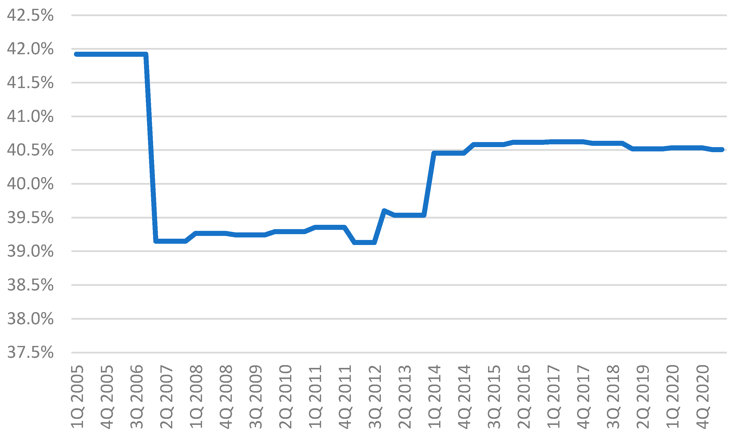
Another caveat in the choice of currency variable and definition of the estimated model is related to the high level of euroization of the economy (for more details see Atanasijević and Božović [41]). Apart from the foreign currency deposits, which constitute about 75% of citizens’ savings and approx. 62% of all deposits (57% of M3), Figure 2, there is a certain amount of foreign currency in cash that citizens keep in their homes. Some estimates based on a survey conducted by the Austrian central bank [42] show that Serbia has one of the highest rates of currency substitution measured by the share of foreign currency cash in total cash in circulation in Central, Eastern, and Southeastern Europe regions, at about 45% in 2019–2020, corresponding to the per capita amount of about 230 euro holding.

Unlike foreign currency deposits in banks, this foreign currency cash money is not registered or included within official monetary statistics. Therefore, it remains outside of the scope of our estimated dependent variable, which measures the real amount of currency in circulation. The Serbian Dinar is a legal tender in the economy and is used for almost all transactions with only a few exceptions. The law permits the use of foreign currency for payments related to purchasing of real estate and cars. Moreover, similar to foreign currency deposits, the stocks of foreign currency kept at homes serve primarily for the store of wealth function of money rather than for transactions. This is mostly due to psychological reasons related to the history of hyperinflation and very unstable exchange rates of local currency during several decades, which left consequences on the behaviour of citizens related to the credibility of local currency as a store of value.

A positive aspect of the previous caveat on our dependent variable (measured as local currency) is that it represents a clearer aggregate, i.e., the amount of transaction cash money—the one described by the currency demand function, which we estimate by our model. Thus, estimating the shadow economy using the currency demand approach in the case of Serbia, is more appropriate in terms of cash variable than for countries where the estimated cash in circulation variable includes the cash held for precautionary purposes, which has been registered to vary due to the changes in the behaviour of citizens over the observed period in EU countries [43]—the phenomena which may render the results of the estimated model quite ambiguous.

Nonetheless, we are aware that there may still be some cash in foreign currency used in transactions that belong to the shadow economy and that we want to assess, but it is not captured by the estimated excess currency from our model. In this context, we assume that the amount of cash in foreign currency used for transactions (that belong to the shadow economy) is relatively smaller than the domestic currency in circulation. In the final estimation, the consequent underestimation of the excess cash is somewhat compensated by the overestimation of the money velocity. The latter would be smaller if the transaction money in foreign currency cash were calculated as part of M1, i.e., part of C (due to an increase in the denominator of the Y/M1 ratio). As a result, the final share of the shadow economy in GDP would stay at a similar level.

3.3. Choice of the Variable Tax Rate Measuring Fiscal Burden

As addressed throughout the literature [44], the choice of the proxy variable to measure the fiscal burden, i.e., an incentive to conduct unregistered business, represents another practical challenge related to the currency demand approach.

Similar to prior studies using the currency demand approach for other countries, mentioned in Section 2.2, in this study, we examined several different alternative measures for this variable, notably considering the evolution of the tax system in Serbia over the observed period.

The most satisfying result, upon which we based our calculations of the final indicator of the informal economy, was obtained using an originally constructed variable to encompass the changes in the tax burden on personal income and VAT rate as the two most important taxes motivating unregistered business transactions (Tax_1). We constructed this variable by taking the official value of the consumer basket for the observed period. The official consumer basket is defined according to the methodology prepared by the Statistical Office of the Republic of Serbia (SORS) in line with Eurostat’s methodological principles. It is calculated and published regularly by the Government of Serbia by the ministry in charge of trade. We further calculated the value of income tax and contribution that would have to be paid for the equivalent net personal income according to the ruling taxing for the observed period. We added to that amount the value of VAT included in the equivalent consumption by applying the ruling VAT rates for the period in question. Finally, the constructed tax rate was obtained as a proportion of the sum of these two types of taxes and the equivalent gross income corresponding to the value of the consumer basket. Thus, our originally created variable represents a much more accurate indicator of the tax burden than any of the existing aggregate ratios dominantly used in the literature.

Following the literature, however, we estimated alternative models with a few different tax variables calculated as ratios of tax revenue or government spending to GDP. We ran the model using the overall tax revenue to GDP (Tax_2). This variable was less reliable as it is, to some extent, distorted in measuring fiscal burden by the government’s effort to reduce the shadow economy and improve tax collection—which is unevenly distributed over the observed period. The explicit government policy aiming to reduce the shadow economy and improve tax collection was on the agenda after a stiff fiscal consolidation program was introduced in 2014 and lasted over a few consecutive years. Since 2015, the Serbian Government has undertaken an explicit policy to reduce the grey economy initiated by large private companies. It enacted a set of specific measures as part of an action plan lasting from 2015 to 2020 [45], which was followed by another action plan [46]. At the same time and in line with the process of the modernization and digitalization of public services, a comprehensive plan for transforming and modernizing tax administration was implemented in 2019 [47]. The latter was agreed upon and monitored as part of an arrangement with the International Monetary Fund [48] and included the development of a strategic risk management function within the Tax Administration of Serbia which is meant to rely extensively on big data analytics.

Further following the literature, we tried using separate proxy variables for direct taxes. Thus, we used collected personal income tax to GDP (variable Tax_3) and collected personal income tax and contributions to GDP (variable Tax_4). The last two variables perform less well, which is probably due to possible multicollinearity. Namely, there is a negative correlation between variables Tax_3 and Tax_4 and variable GDP as there were two significant cuts in personal income burden in the periods of prolonged GDP growth over the observed period. The variable Tax_5 measures government expenditure to GDP, which, besides capturing the desired effect of changing fiscal burden, was in parallel changing over the observed period in line with the level of fiscal policy restrictiveness and access to funds (mostly debt) for financing the fiscal deficit (

Table 1. Variables correlation matrix.

	CR	GDP	Tax_1	Tax_2	Tax_3	Tax_4	Tax_5	i
CR	1.00
GDP	0.870 *	1.00
Tax_1	0.150	0.004	1.00
Tax_2	0.459 *	0.277 *	0.489 *	1.00
Tax_3	−0.425 *	−0.506 *	0.162	0.203	1.00
Tax_4	0.006	−0.124	0.247	0.634 *	0.748 *	1.00
Tax_5	0.305 *	0.240	−0.136	0.105	0.199	0.360 *	1.00
i	−0.652 *	−0.468 *	−0.611 *	−0.641 *	0.260 *	−0.103	0.069	1.00
FX_rate	0.558 *	0.584 *	−0.137	−0.082	−0.831 *	−0.568 *	−0.018	−0.243

Note: star (*) correspond to 0.05 probability level

).

4. Results and Discussion

As mentioned, the cointegrating vector $\mathit{\beta }$ from the VECM was used to obtain the relationship between the variables. The vector was normalized in relation to the first variable, Cr. For the sake of clarity, the vectors $-\mathit{\beta }=\left[1,{\alpha }_0,{\alpha }_1,{\alpha }_2,{\alpha }_3,{\alpha }_4 \right]$ are shown in

Table 2. Estimates of the long-run cointegration relation.

Model		(1)	(2)	(3)	(4)	(5)
trace statistic	5%	2	2	1	2	2
	1%	1	1	1	1	1
max eigenvalue-statistic	5%	2	2	1	2	2
	1%	1	2	1	2	2
GDP		2.107 (0.130) ***	2.114 (0.123) ***	2.462 (0.161) ***	2.301 (0.181) ***	2.053 (0.096) ***
Tax_1		1.640 (0.803) **
Tax_2			3.932 (1.381) ***
Tax_3				6.919 (2.248) ***
Tax_4					5.913 (1.941) ***
Tax_5						0.535 (0.699)
i		−0.0073 (0.004) **	0.0025 (0.005)	−0.0092 (0.003) ***	−0.0042 (0.0044)	−0.011 (0.003) ***
C		0.203 (0.034) ***	0.075 (0.043) *	0.123 (0.038) ***	−0.0811 (0.055)	0.179 (0.041) ***
const		−20.343	−19.495	−23.346	42.709	17.577
log likelihood		421.28	400.84	485.43	440.13	352.56
chi2		778.88	438.58	684.02	228.05	834.63

All models estimated assume one cointegrating equation. The number of lags in the model were determined using SBIC. Model was estimated using two lags. Standard errors are in parentheses. * p < 0.10 ** p < 0.05 *** p < 0.01.

for each model. As expected, in model (1), which corresponds to Equation (3), the overall level of income (measured by GDP) had a positive significant impact on the level of currency with the most important coefficient compared to other variables. A similar level of the coefficient stands in all model specifications. The tax burden proxy ($Tax\_1$) had a proportionally less important level with a positive and significant impact, in line with the expectation based on the theoretical model. A similar observation stands for the interest rate on local currency deposits while the coefficient, as expected, had a negative sign indicating that a higher opportunity cost of holding cash (interest rate on bank deposits) induced a lower level of currency in circulation. The dummy variable for the COVID-19 pandemic period, which was marked by lockdown and change in behaviour related to spending and related payments, yielded a positive and significant coefficient estimate. The model diagnostics and robustness check is presented in Appendix A.

After estimating the vector error correction model (VECM) and obtaining the coefficients for the long-run relationship, we used the estimated equation for version (1) of the model to calculate the estimated level of real cash in circulation $\widetilde{CR}$:

$${\widetilde{CR}}_t=-20.343+1.640·Ta{x}_1{}_t+2.107·GD{P}_t-0.0073·i_t+0.203·C_t$$

(5)

To determine the amount of extra currency (EC), we first estimate the $\widehat{CR}$ by setting the “no-informal economy” value of the incentive variable related to fiscal burden. We followed the principle of the approach by Dybka et al. [28] and Hernandez [25] that a zero tax rate should not be applied as it represents an unrealistic assumption. However, we considered that the use of the historical minimal rate, as applied by these authors, for the level of the incentive variable would result in the absence of the shadow economy and would also be unrealistic for the case of Serbia as the general level of measured fiscal burden is relatively high over the observed period despite some variations (Figure 3). For that reason, we opt for this purpose to set the minimal (average tax) rate at which there would be no shadow economy at 10%. This corresponds with the rate which is well known and acceptable minimal charge on the “market” for translating deposit into “legally taxed” cash (and vice versa, for a kind of (cash) money laundering i.e., translating it into usable deposit since firms owning illegal cash are not allowed to make any payment in cash except for some small charges).

The difference $\widetilde{CR}-\widehat{CR}$ gives EC (excess cash) used for all kinds of shadow activities in the economy. According to Tanzi [13], we assumed the velocity was the same in both formal and informal sectors, and we estimated the level of real informal income $Y_H$. Further on, we calculated the share of the informal economy in the total economy. Following Ahumada et al. [35], we proceeded to correct our estimates using their suggested method (Equation (3)). Equation (3) provides an expression for ${\widehat{Y}}_H$ given $Y_R$, estimated $C{R}_R,$ and $C{R}_H$ using the model specification in Equation (5) and $\beta ={\widehat{\alpha }}_2$ = 2.107.

The obtained indicator showed a downward trend over the overall period. However, after a steep decline in the expansionary period prior to the global crisis, the pre-crisis level of about 25% had risen afterward to 27% by the end of 2011. The subsequent visible decrease for the indicator began in 2014 and has lasted to date, where it reaches just below 20%. That period, as already mentioned, was marked by the government’s determination to fight the shadow economy using several targeted measures. However, the level of the hidden economy seems to appear relatively high (Figure 4).

Our results responding to our main research question on the level and trend of the shadow economy in Serbia revealed that it attained roughly 20% of GDP by the end of Q3 of 2021 and that it has been gradually decreasing from approx. 30% of GDP at the end of 2005. This trend could be explained by the country’s approximation process to the European Union and related harmonisation of the domestic legislation and fiscal consolidation coupled with the IMF program from 2014, including the modernization of tax administration and other targeted measures to reduce the shadow economy by several successive governments.

In comparison to the other methods applied for the Serbian case, the currency demand approach-based method consistently reported lower levels of the shadow economy than the MIMIC-based model—which is expected and reported in the literature [2]. Indeed, MIMIC-based models often take into account all institutional sectors and all types of informal activity [10] and thus are normally considered as upper-bound in comparison to other methods. In our case, our model shows that the shadow economy in 2008 stood at approx. 24% of GDP, against 26.2%, reported by a MIMIC model [8,10]. The gap between the two models persisted, with the gap reaching 4.7 percentage points in 2009 and 3.3 percentage points in 2010.

On the other hand, the currency demand approach-based model reported consistently higher levels of the shadow economy than the direct method-based method—which is, again, expected and reported in the literature [2], as this type of model tends to capture shadow economy activities very partially. For example, they often exclude some forms of informal labour, or only include formally registered companies, or it might, for instance, exclude the household sector [10], thus leaving some of the shadow economy activity out of the scope of the model. As a result, our model reported that the shadow economy reached about 25% of GDP in 2014, against 23.5% reported by the direct method-based model. The gap also persisted, with the gap reaching as much as 6.8 percentage points in 2017 [8].

In terms of relevant regional comparison, our results are similar to the obtained estimated level and trend of the shadow economy in Bulgaria using the comparable monetary approach [30]. Petranov et al. found that the shadow economy in Bulgaria for the period 2006–2019 tended to decline: from 31.7% of GDP to 21.1% of GDP. On the other side, the current estimated level of the shadow economy in Serbia at about 20% corresponds to the estimated average EU countries level in the 1980s using the currency demand approach [49], while the most similar result corresponds to Spain in the same period [49,50].

Apart from addressing the key research question, our paper also provides an originally constructed indicator for fiscal burden encompassing the effect of the changes in both direct and indirect taxes, i.e., from personal income tax and VAT rate—the two most important tax forms. As previously specified, we constructed this novel variable by taking the official value of the consumer basket for the observed period and calculated the value of income tax and contribution needed to be paid for the equivalent net personal income. This indicator performed much better as it did not suffer from some of the problems as the proxies for tax rate dominantly used in the literature and calculated using aggregates such as collected tax revenue to GDP or government expenditure to GDP. Thus, we somewhat contributed to addressing the issue of the measurement of fiscal burden, which is widely recognised in the literature related to the currency demand approach.

5. Concluding Remarks

This pioneering application of the cash demand method to the Serbian case provided additional insights into the nature, level, and trends of the shadow economy and its activities in Serbia over the past two decades. Its key contribution relates to the construction of a novel indicator, providing new insight into the level and dynamic of the shadow economy in Serbia. Our indicator showed that Serbia’s shadow economy has gradually decreased to approximately 20% of GDP in 2021, down by almost 10pp since 2005. This also included two reversal episodes within this period—in the aftermath of the 2008 global financial crisis, i.e., in the early 2010s, and in the aftermath of the COVID-19 pandemic.

Thanks to the nature of the approach, which relies on publicly available data and is a relatively objective way to indirectly assess the unregistered economic activity by estimating the excess cash in use, this indicator provides an integral overview of the level and dynamic of the shadow economy in Serbia—reporting its levels for each quarter between 2005 and 2021. This represents a significant contribution to the understanding of the shadow economy by complementing the results obtained using the other estimation methods—which tend to provide only sporadic and less objective results for the same period.

Our results convey at least two important proposals relevant to policy formulation. Firstly, the authorities could put in place an annual or quarterly monitoring of the shadow economy, which can be easily produced based on the public data available, with a lag of one to two quarters. Thus, the observed changes in its level and trend may be a valuable input for policymakers as well as their tool in tracing the effects of their policy on the relative level of the shadow economy.

Secondly, our results show a relatively high level of the income elasticity of cash in circulation for the relative level of income per capita in Serbia, which may represent a valuable insight for policymakers. Namely, a further investigation should be directed to understand the underlying factors that result in the higher than unitary income elasticity of the currency in circulation. These factors could be rooted in some regulation or behaviour patterns which could, in turn, be targeted by specific policy measures.

However, it should be underlined that this approach contains certain limitations. First, it strives to measure the income that is only generated through the excessive use of currency, which was hidden from the tax authorities, i.e., unregistered. Yet, the actual size of the informal sector may be even larger if some other incentives to hide economic activity were included (e.g., the illegal economy). Thirdly, our results are somewhat distorted as we only looked at the Serbian Dinar-denominated part of the informal transactions, while some part of the shadow economic activity could be realized by foreign currency cash payments.

Moreover, the model could be improved in the future by including a few other relevant factors influencing the level of currency in circulation, such as technology adoption for cashless payments and switching to online purchases. This will become possible once the time span broadens to cover a longer series of available data on payment behaviour and online consumption, which starts from as early as 2016. The longer data series will also allow the introduction of some measure of the regulatory burden in the estimated model.

Having all the previously stated in mind, and given the degree of uncertainty around the estimates, the presented results should be taken as an approximation of the size and trend of the shadow economy rather than as its precise measure.