Study on Noise Correction Algorithm of Infrared Emissivity of Rock under Uniaxial Compression

Abstract

In the process of uniaxial loading of rocks, the original temperature information of infrared radiation is easily submerged in the noise signal, which leads to distortion of the obtained infrared radiation response information. In this paper, we propose a multi-band pseudo-emissivity denoising algorithm. Based on the basic theory of infrared radiation, by separating the infrared temperature measurement from the emissivity of the measured object, we constructed an infrared multi-band temperature measurement vector group that does not involve the emissivity to reduce the noise interference caused by the infrared temperature measurement results and the emissivity. Under a loading experiment of rock under uniaxial compression, the change of infrared radiation (IR) characteristics with loading was observed. The research results show that the multi-band pseudo-emissivity algorithm could effectively denoise infrared images and, using the denoised rock surface MIRT, AIRT and IRV as indicators, the characteristics of infrared radiation change in the process of uniaxial compression loading and fracturing of real rocks were analyzed.

1. Introduction

Large-scale continuous mining of coal mines over the years has led to the depletion of shallow coal resources, and mineral resources have gradually entered the deep mining stage [1,2,3,4,5]. When coal is mined at greater depth, the frequency of coal rock dynamic disasters rises, which seriously affects mine production safety. During the process of rock deformation and damage abundant radiation energy, such as acoustic radiation and electromagnetic radiation, is released. The use of advanced monitoring technology has become common practice to understand the process of rock damage [6,7,8,9]. As a real-time, non-destructive, non-contact monitoring technology, infrared thermography provides a new perspective for understanding the loading damage of rocks [10,11,12,13,14,15].

In the past several decades, many scholars have studied the properties of infrared radiation during rock loading, and have accumulated abundant results. Deng [16] found experimentally that infrared radiation varies with the stress state during the loading of rocks. Wu conducted mechanical experiments and made infrared radiation observations for different types of rocks under laboratory conditions [17,18,19]. Ma investigated the connection between microscopic changes, mechanics and infrared radiation characteristics during rock fracture [20,21,22]. Freund proposed that infrared radiation is generated due to the excitation of cavity charges inside rocks under stress to form electric currents emitting electromagnetic radiation [23]. Luong MP studied the infrared thermal characteristics of different types of rocks during fracture [24]. Grinzato studied the infrared thermographic characterization of rock fractures [25].

When monitoring the damage and fracture of coal and rocks using infrared radiation technology, the infrared radiation information is easily affected by the emissivity, measurement angle and ambient temperature [26,27,28,29,30]. The low amplitude of infrared radiation temperature change during the evolution of rock damage results in the original temperature information of infrared radiation being easily drowned in the noise signal, which in turn makes the experimental results unreliable [31,32,33,34,35,36,37,38]. This greatly affects the application of infrared radiation technology in mining, and in the field of rock mechanics. It is particularly important to eliminate or reduce the noise signal in infrared radiation information.

In this paper, we use emissivity to explore the optical mechanism of infrared denoising. Based on the basic theory of infrared radiation, an infrared denoising algorithm is proposed. By separating the infrared temperature measurement from the emissivity of the measured object, an infrared multi-band temperature measurement vector group that does not involve emissivity is constructed to solve the problem of low coupling between infrared temperature measurement results and emissivity. The denoising effect is analyzed, and the temperature variation characteristics of the coal uniaxial compression infrared radiation after denoising are obtained.

2. Infrared Emissivity Denoising Algorithm

The general basic equation for thermal infrared imager radiation temperature measurement can be expressed as:

$$f(T_0^{\prime })={\tau }_a[\epsilon f(T_0)+(1-\alpha )f(T_u)]+(1-{\tau }_a)f(T_a)$$

(1)

where f(x) is the expression of radiation temperature measurement of the infrared thermal imager. $T_0^{\prime }$ is the surface temperature of the measured object, T₀ is the real temperature, T_u is the ambient temperature, T_a is the atmospheric temperature, ε is the emissivity, α is the absorption, and τ_a is the atmospheric transmittance.

The actual temperature of the measured object is:

$$f(T_0)=\frac{1}{\epsilon {\tau }_a}[f(T_0^{\prime })-{\tau }_a(1-\alpha )f(T_u)-(1-{\tau }_a)f(T_a)]$$

(2)

In Equation (2), the true temperature of the object being measured is affected by the emissivity of the object surface, atmospheric transmittance, surface absorption, ambient temperature, atmospheric temperature and radiation temperature of the object surface temperature. Because most infrared thermal image measurements are short-range measurements, τ_a = 1 can be taken [39,40,41]. Equation (2) becomes:

$$f(T_0)=\frac{1}{\epsilon }[f(T_0^{\prime })-(1-\alpha )f(T_u)]$$

(3)

where the unknown quantities are f(T₀), ε and α. For objects with continuous radiation, the emissivity is ε(λ,T). According to Taylor’s formula, this can be expanded as:

$$\begin{array}{l}\epsilon (\lambda ,T)=\epsilon ({\lambda }_0,T)+\epsilon ({\lambda }_0,T)(\lambda -{\lambda }_0)+\frac{1}{2}{\epsilon }^{″}({\lambda }_0,T)(\lambda -{\lambda }_0)+\\ \dots +\frac{1}{n}{\epsilon }^{(n)}({\lambda }_0,T){(\lambda -{\lambda }_0)}^n+O_n(\lambda )\end{array}$$

(4)

where the residual term O_n(λ) is:

$$O_n(\lambda )=\frac{1}{(n+1)!}{\epsilon }^{(n+1)}({\lambda }_0,T){(\lambda -{\lambda }_0)}^{(n+1)}$$

(5)

Define dimensionless wavelength Λ. The meaning of Λ is a dimensionless constant, which is used to represent the wavelength coverage Λ = (λ − λ_min)/(λ_max − λ_min), where λ_max is the upper limit of the IR camera response band and λ_min is the lower limit of the IR camera response band.

$$\epsilon (\lambda ,T)=a_0(\lambda ,T)+a_1(\lambda ,T)\mathsf{\Lambda }$$

(6)

$$\alpha (\lambda ,T)=b_0(\lambda ,T)+b_1(\lambda ,T)\mathsf{\Lambda }$$

(7)

Equation (3) can be expressed as:

$$f(T_0^{\prime })=\epsilon f(T_0)+(1-\alpha )f(T_u)$$

(8)

Substituting Equations (6) and (7) into Equation (8), the vector group can be constructed:

$$\left[\begin{array}{c}{f}_1(T_0^{\prime })\\ f_2(T_0^{\prime })\\ f_3(T_0^{\prime })\end{array}\right]=\left[\begin{array}{cc}1& {\mathsf{\Lambda }}_1\\ 1& {\mathsf{\Lambda }}_2\\ 1& {\mathsf{\Lambda }}_3\end{array}\right]\times \left[\begin{array}{c}{a}_0\\ a_1\end{array}\right]\times \left[\begin{array}{c}{f}_1(T_0)\\ f_2(T_0)\\ f_3(T_0)\end{array}\right]+\left[\left[\begin{array}{c}1\\ 1\\ 1\end{array}\right]-\left[\begin{array}{cc}1& {\mathsf{\Lambda }}_1\\ 1& {\mathsf{\Lambda }}_2\\ 1& {\mathsf{\Lambda }}_3\end{array}\right]\times \left[\begin{array}{c}{b}_0\\ b_1\end{array}\right]\right]\times \left[\begin{array}{c}{f}_1(T_u)\\ f_2(T_u)\\ f_3(T_u)\end{array}\right]$$

(9)

According to Kirchhoff’s law, the object to be measured is a diffuse reflector; then, there are:

$$b_0(\lambda ,T)+b_1(\lambda ,T)\mathsf{\Lambda }=1-[a_0(\lambda ,T)+a_1(\lambda ,T)\mathsf{\Lambda }]$$

The vector group (9) can be deformed as:

$$\begin{gathered} \left[\begin{array}{c}{f}_1(T_0^{\prime })\\ f_2(T_0^{\prime })\\ f_3(T_0^{\prime })\end{array}\right]=\left[\begin{array}{cc}1& {\mathsf{\Lambda }}_1\\ 1& {\mathsf{\Lambda }}_2\\ 1& {\mathsf{\Lambda }}_3\end{array}\right]\times \left[\begin{array}{c}{a}_0\\ a_1\end{array}\right]\times \left[\begin{array}{c}{f}_1(T_0)\\ f_2(T_0)\\ f_3(T_0)\end{array}\right]+\left[\left[\begin{array}{cc}1& {\mathsf{\Lambda }}_1\\ 1& {\mathsf{\Lambda }}_2\\ 1& {\mathsf{\Lambda }}_3\end{array}\right]\times \left[\begin{array}{c}{a}_0\\ a_1\end{array}\right]\right]\times \left[\begin{array}{c}{f}_1(T_u)\\ f_2(T_u)\\ f_3(T_u)\end{array}\right] \\ {f}_1\left(T_0\right)=f_2\left(T_0\right)=f_3\left(T_0\right), f_1\left(T_{\mathrm{u}}\right)=f_2\left(T_{\mathrm{u}}\right)=f_3\left(T_{\mathrm{u}}\right). \end{gathered}$$

(10)

The vector set has three unknowns, a₁, a₀ and f(T₀), and the matrix can be transposed and deformed to calculate the temperature of the measured object with unknown emissivity.

3. Experiment Design

3.1. Experimental Equipment

SC7300 infrared thermal imager (pixel resolution 320256, pixel pitch 30, thermal imager optional calibration range −20 °C–500 °C). YSSZ-2000 microcomputer-controlled electro-hydraulic servo rock triaxial testing machine (maximum test force: 2000 kN, displacement measurement range: 0–200 mm, displacement resolution: 0.01 mm.)

3.2. Experimental Preparation

Experimental samples were collected from Hunan Province, China. The samples were processed into a size of Φ50 mm×100 mm, and the error of the end face non-parallelism and non-uniformity was less than 0.05 mm [42,43,44,45,46,47,48,49,50]. There were four samples in total. Physical parameters and test results of the samples are listed in

Table 1. Physical parameters and test results of samples.

Sample No.	Emissivity	Density/g/cm3	Poisson’s Ratio	Uniaxial Compressive Strength/MPa	Elastic Modulus/GPa
A	0.85	2.35	0.2	38.34	10.26
B	0.87	2.34	0.19	32.45	9.43
C	0.83	2.34	0.2	32.83	9.52
D	0.84	2.36	0.21	28.76	8.71

.

In order to eliminate the impact of environmental interference, a paper isolation box with a length of 1 m and a width of 0.8 m was prepared. The sample was first placed in the laboratory for more than 24 h to ensure that the temperature of the rock sample was equal to room temperature. It was ensured that the instrument could be used normally and the instrument was started before the test. Both ends of the specimen were coated with butter to reduce end effects during uniaxial compression.

3.3. Experimental Process

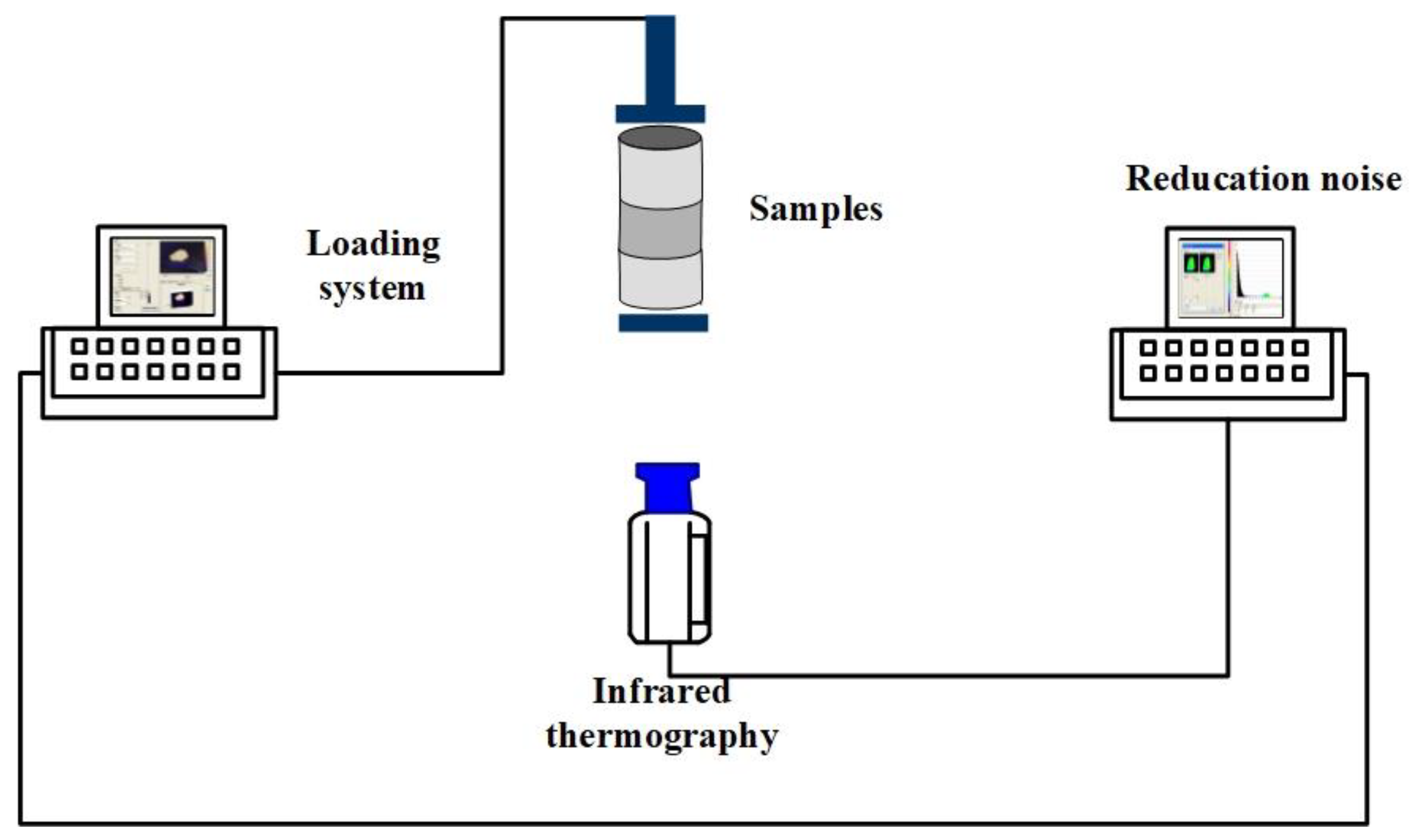
A schematic diagram of the experimental setup is shown in Figure 1. Loading the samples until rupture, the infrared thermal imager was used to observe the infrared radiation dynamics of the test surface during the loading process [43,44,45]. The collected infrared radiation information was applied to the denoising algorithm to optimize the denoising. This experiment yielded basic data and images to provide the basis of infrared radiation response mechanism in the process of bearing coal rock damage.

4. Infrared Radiation Data Processing and Indicators

We recorded both mechanical data and infrared radiation data. Due to the discrete nature of the experimental results, the most representative data in the test specimens were isolated. Data analysis included the calculation and analysis of the strain field and infrared images of the connected rock specimens. The raw infrared image is a representation of the IRT data matrix.

The IRT data in the test area were converted to CSV files by the software. The CSV data sheet could be converted into a temperature matrix using Python software. The expression of IRT data in frame p is shown in Equation (11):

$$f_p(x,y)=\left[\begin{array}{cccc}{f}_p(1,1)& f_p(1,2)& \dots & f_p(1,N)\\ f_p(2,1)& f_p(2,2)& \dots & f_p(2,N)\\ \dots & \dots & \dots & \dots \\ f_p(M,1)& f_p(M,2)& \dots & f_p(M,N)\end{array}\right]$$

(11)

where p is the frame index of the infrared image sequence, and x and y are the rows and columns of the thermal recorder temperature matrix, respectively. M and N are the maximum number of rows and columns in x and y, respectively.

It is important to note that IRT is the radiant temperature of the target surface, not the true physical temperature.

At this time, the acquired infrared data are obviously related to the emissivity. In order to obtain more accurate infrared data, the multi-band pseudo-emissivity algorithm was first used to correct the data matrix and obtain a temperature matrix unrelated to the emissivity. Python software was then applied to extract the relevant IR indicators (MIRT, AIRT and IRV). The parameters representing IRT in this area mainly include the maximum infrared radiation temperature (MIRT), the average infrared radiation temperature (AIRT) and the infrared radiation variance (IRV).

The processing of infrared thermal images and the extraction steps of indicators are shown in Figure 2.

MIRT refers to the highest temperature in the regional temperature field. AIRT reflects the overall intensity of regional infrared radiation. IRV can reflect the dispersion degree of the infrared radiation temperature value on the entire rock surface, and can be obtained by calculating the variance of the infrared radiation thermal image sequence matrix.

$$MIRT=\max f_p(x,y)$$

(12)

$$AIRT=\frac{1}{M}\frac{1}{N}{\displaystyle \sum _{y=1}^N{\displaystyle \sum _{x=1}^M{f}_p(x,y)}}$$

(13)

$$IRV=\frac{1}{M}\frac{1}{N}{{\displaystyle \sum _{y=1}^N{\displaystyle \sum _{x=1}^M[f_p(x,y)-AIRT]}}}^2$$

(14)

where p is the frame index of the infrared image sequence and x and y are the rows and columns of the thermal recorder temperature matrix, respectively. M and N are the maximum number of rows and columns in x and y, respectively.

5. Experiment Results

5.1. Infrared Thermogram

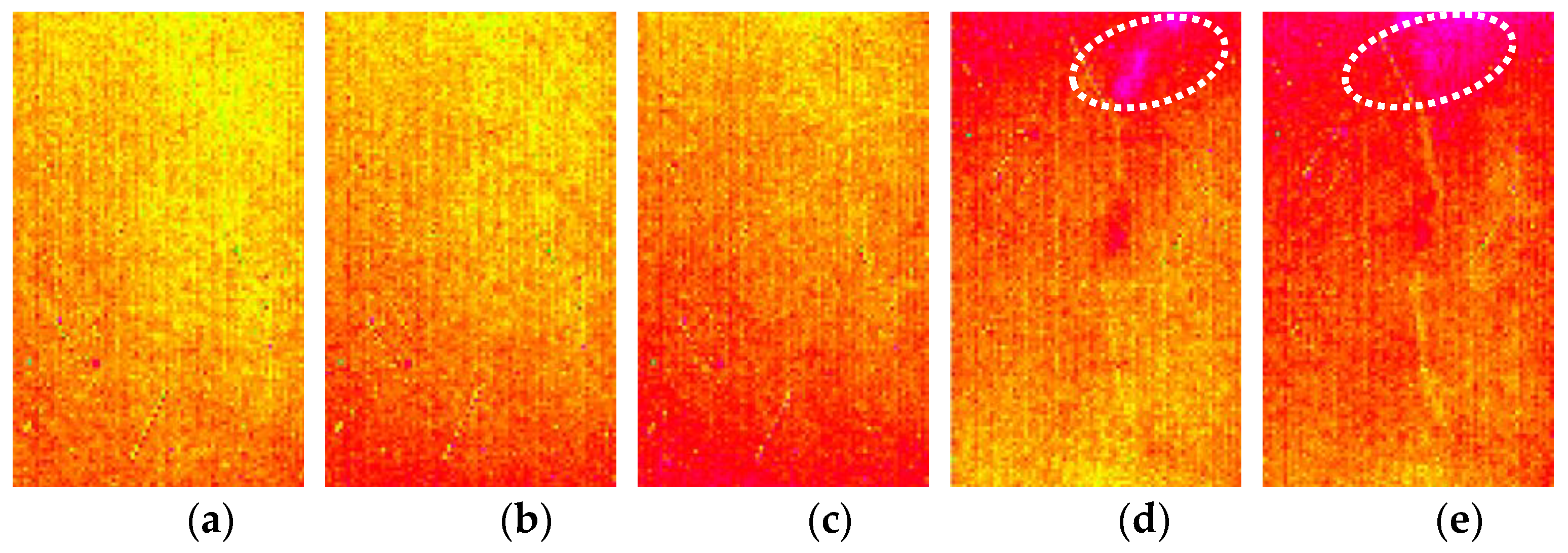
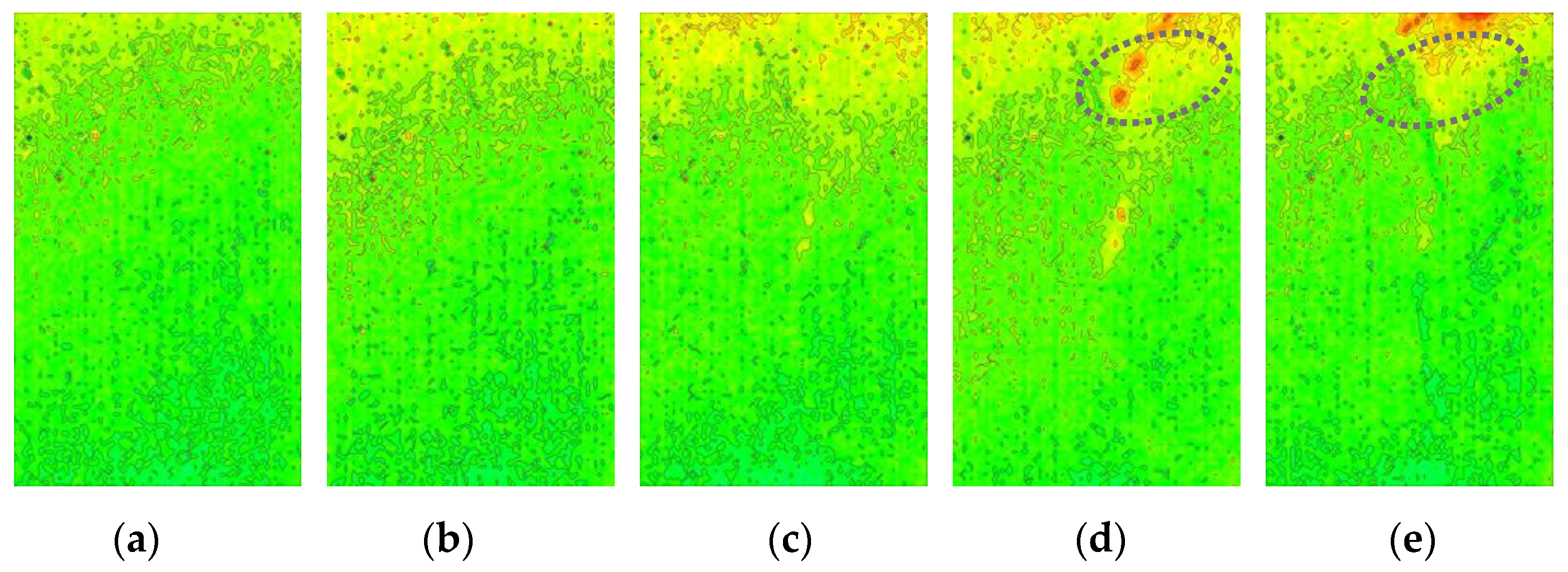
IRT reflects the dispersion degree of infrared radiation temperature on the rock surface. In order to analyze the spatial distribution and change of infrared radiation of rock samples during the loading process, the original infrared radiation data on the rock surface were extracted, and the data matrix was corrected by applying the multi-band pseudo-emissivity algorithm to obtain infrared cloud images that are not related to emissivity. Due to restricted sample space, only Sample A is analyzed in this paper. Figure 3 is the original infrared image of rock Sample A and Figure 4 is the infrared image after noise reduction of rock Sample A.

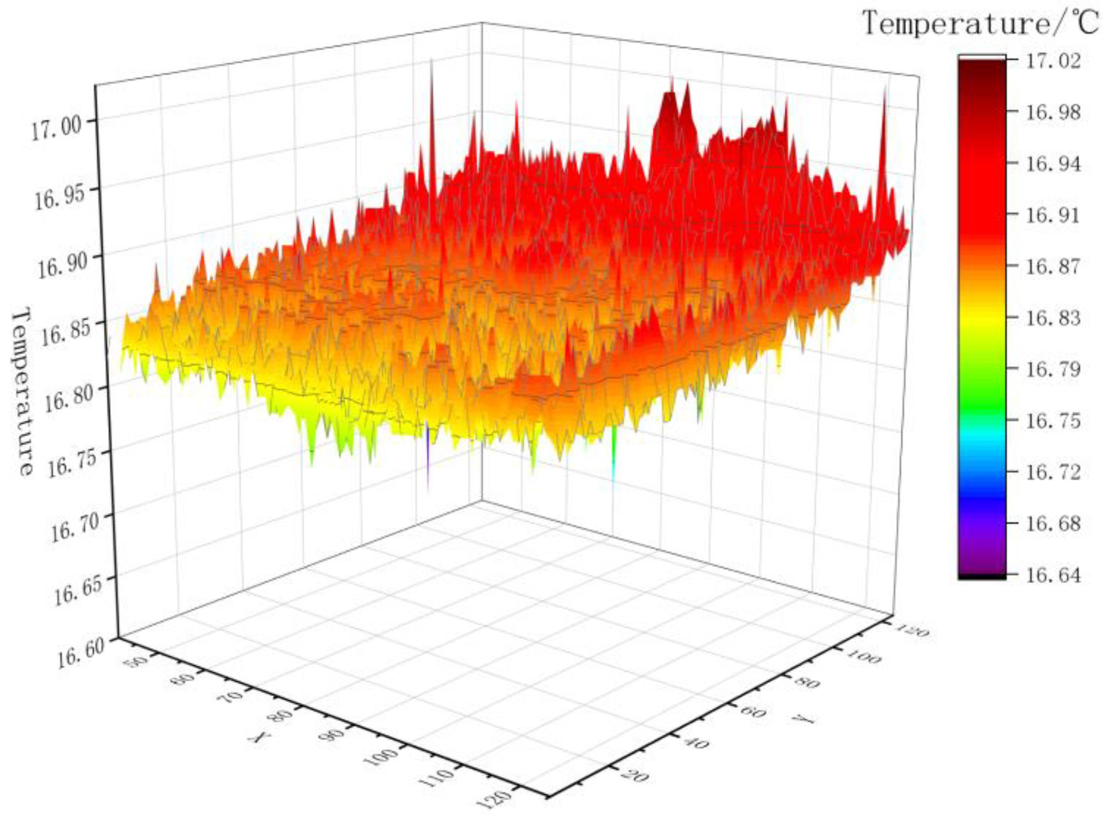
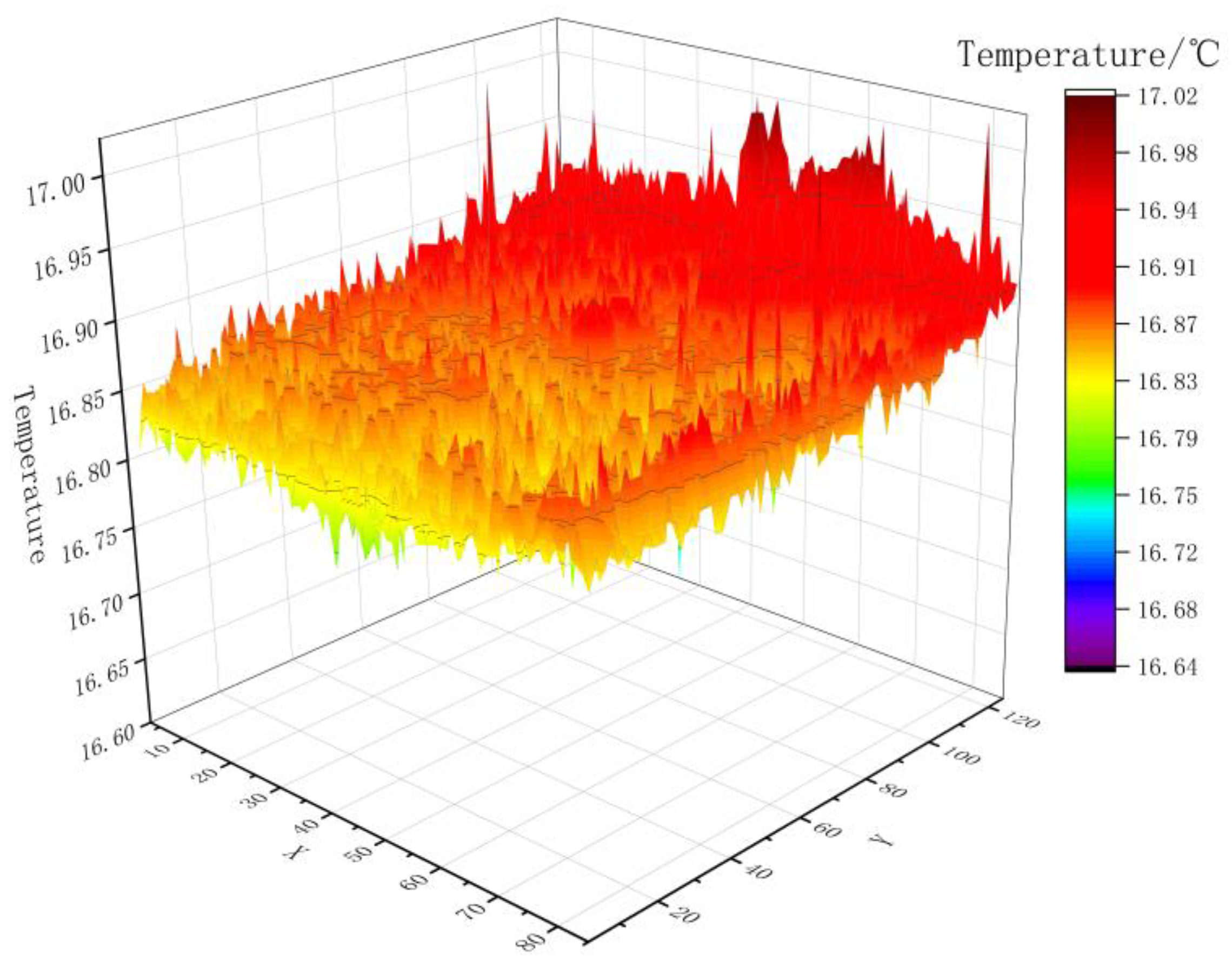
According to related studies, abnormal high-temperature areas will appear in infrared images during rock loading damage. Comparing Figure 3 and Figure 4, the change in the high-temperature area in the original infrared image is not particularly obvious because of the influence of the original emissivity of the rock. In the infrared image after noise reduction it can be observed that the abnormal high-temperature area gradually appears from the beginning of loading, and the bright band becomes increasingly obvious until it breaks. In order to further compare the difference between the infrared images before and after noise reduction, an infrared 3D cloud map was made. Figure 5 is the original infrared image cloud map at 800 s, while Figure 6 is the infrared image cloud map after noise reduction at 800 s. Comparing Figure 5 and Figure 6, it is apparent that the abnormal high-temperature area fluctuates more obviously after noise reduction.

5.2. Indicator of MIRT

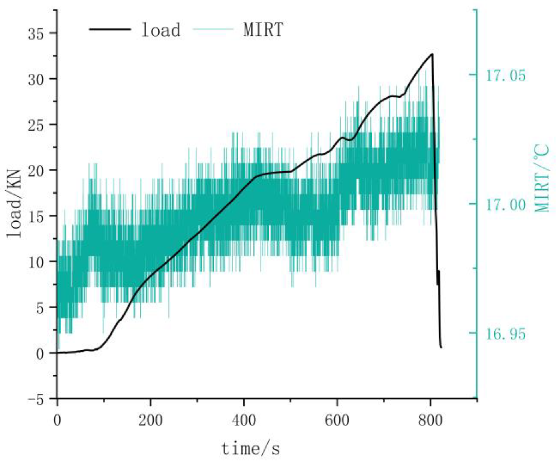
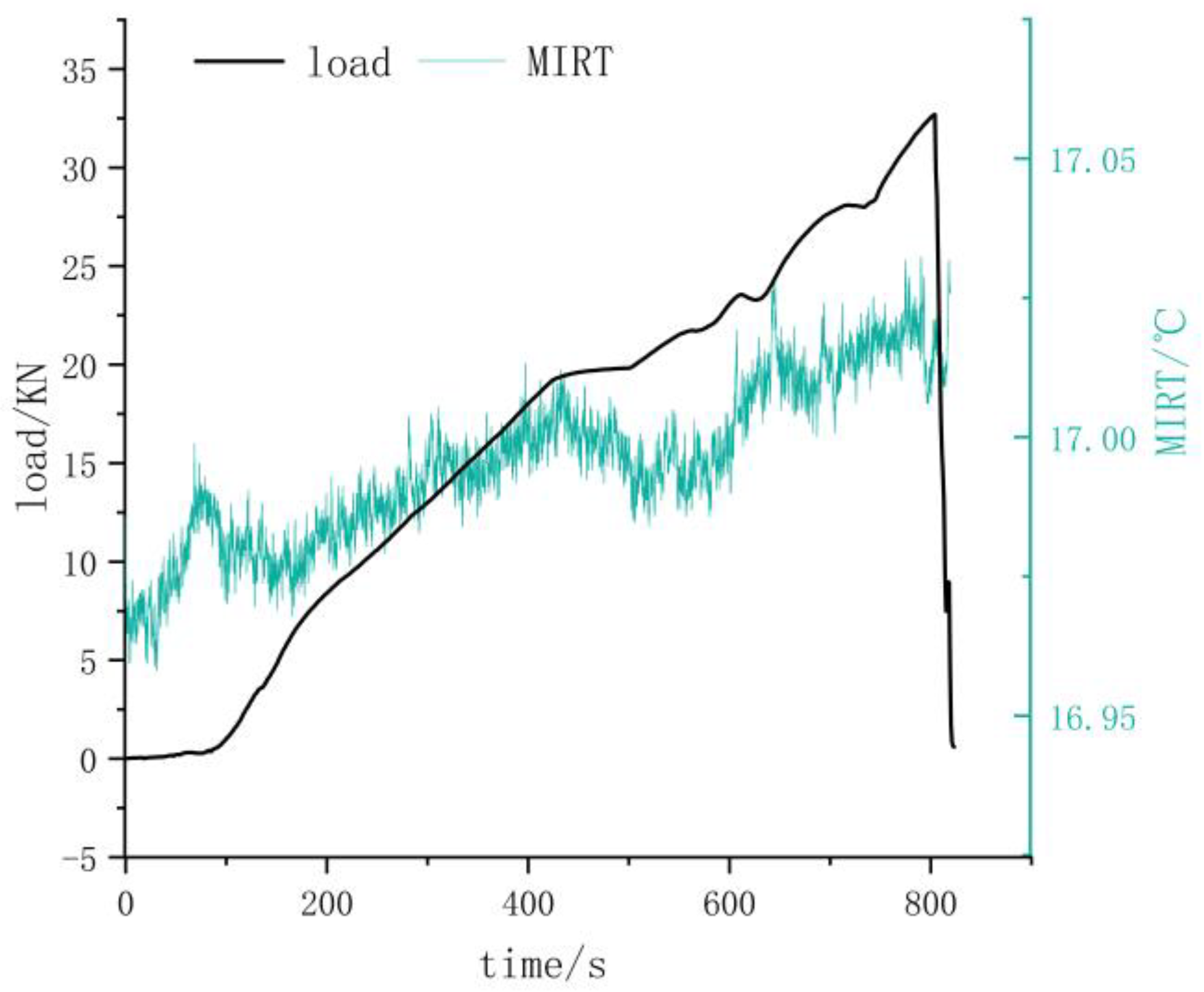
There was a correlation between MIRT and stress during the uniaxial loading of rocks. Due to the restricted sample space, only Sample A was selected for image analysis. Figure 7 shows the MIRT–load time curve without denoising, Figure 8 is the MIRT–Load time curve after algorithm noise reduction. During the loading process, the MIRT exhibits a step-by-step heating pattern as a whole over time. The rise is small, and only changes significantly at the moment of destruction. In Figure 7, the temperature increases from 16.92 °C to 17.02 °C—an increase of 0.1 °C. In Figure 8, the temperature increases from 16.98 °C to 17.03 °C—an increase of 0.05 °C. Comparing Figure 7 and Figure 8, it is clear that the fluctuation range of the MIRT data after noise reduction processing is more precise.

For further comparative analysis, the MIRT data of the samples were fitted. The fitting functions for samples are as follows. The degree of fitting of the formula is shown in

Table 2. Degree of fitting of the formula.

Sample	Degree of Fitting of the Formula
	Before Denoising	After Denoising
A	0.6413	0.8428
B	0.4295	0.5173
C	0.6111	0.6134
D	0.5726	0.5180

.

For Sample A, the MIRT fitting relation before denoising is:

f(x) = 16.967 + 3.653*10⁻⁶*x + 8.8511*10⁻¹⁰*x² − 1.7773*10⁻¹³*x³ + 8.9928*10⁻¹⁸*x⁴.

The MIRT fitting relation after denoising is:

f(x) = 16.967 + 3.6697*10⁻⁶*x + 8.7422*10⁻¹⁰*x² − 1.7589*10⁻¹³*x³ + 8.9018*10⁻¹⁸*x⁴.

For Sample B, the MIRT fitting relation before denoising is:

f(x) = 16.871 − 2.4253*10⁻⁶*x + 1.7748*10⁻⁹*x² − 2.2831*10⁻¹³*x³ + 9.1538*10⁻¹⁸*x⁴.

The MIRT fitting relation after denoising is:

f(x) = 16.968 + 4.1492*10⁻⁶*x + 2.0841*10⁻¹¹*x² − 2.5144*10⁻¹⁴*x³ + 1.4767*10⁻¹⁸*x⁴.

For Sample C, the MIRT fitting relation before denoising is:

F(x) = 16.905 + 2.2722*10⁻⁶*x + 6.8655*10⁻¹⁰*x² − 1.0916*10⁻¹³*x³ + 5.0192*10⁻¹⁸*x⁴.

The MIRT fitting relation after denoising is:

f(x) = 16.694 + 2.7602*10⁻⁶*x + 4.9095*10⁻¹⁰*x² − 6.233*10⁻¹⁴*x³ + 2.3735*10⁻¹⁸*x⁴.

For Sample D, the MIRT fitting relation before denoising is:

F(x) = 16.599 + 7.2586*10⁻⁶*x−1.8187*10⁻⁹*x² + 2.3396*10⁻¹³*x³ − 9.0388*10⁻¹⁸*x⁴.

The MIRT fitting relation after denoising is:

f(x) = 16.968 + 4.1320*10⁻⁶*x + 2.8111*10⁻¹¹*x² − 2.6187*10⁻¹⁴*x³ + 1.5240*10⁻¹⁸*x⁴.

From the above fitting data of four samples, it can be seen that the fluctuation trend of MIRT was more concentrated after denoising.

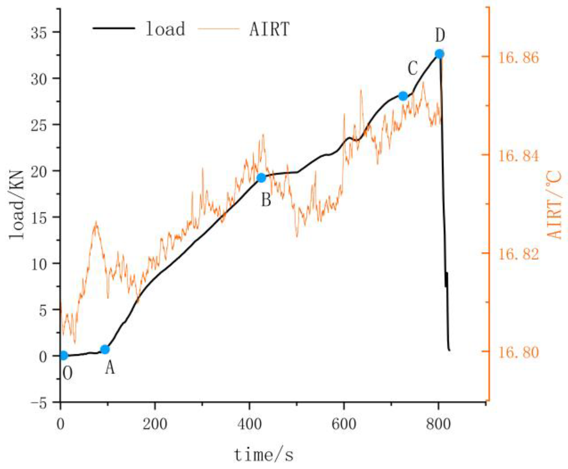
5.3. Indicator of AIRT

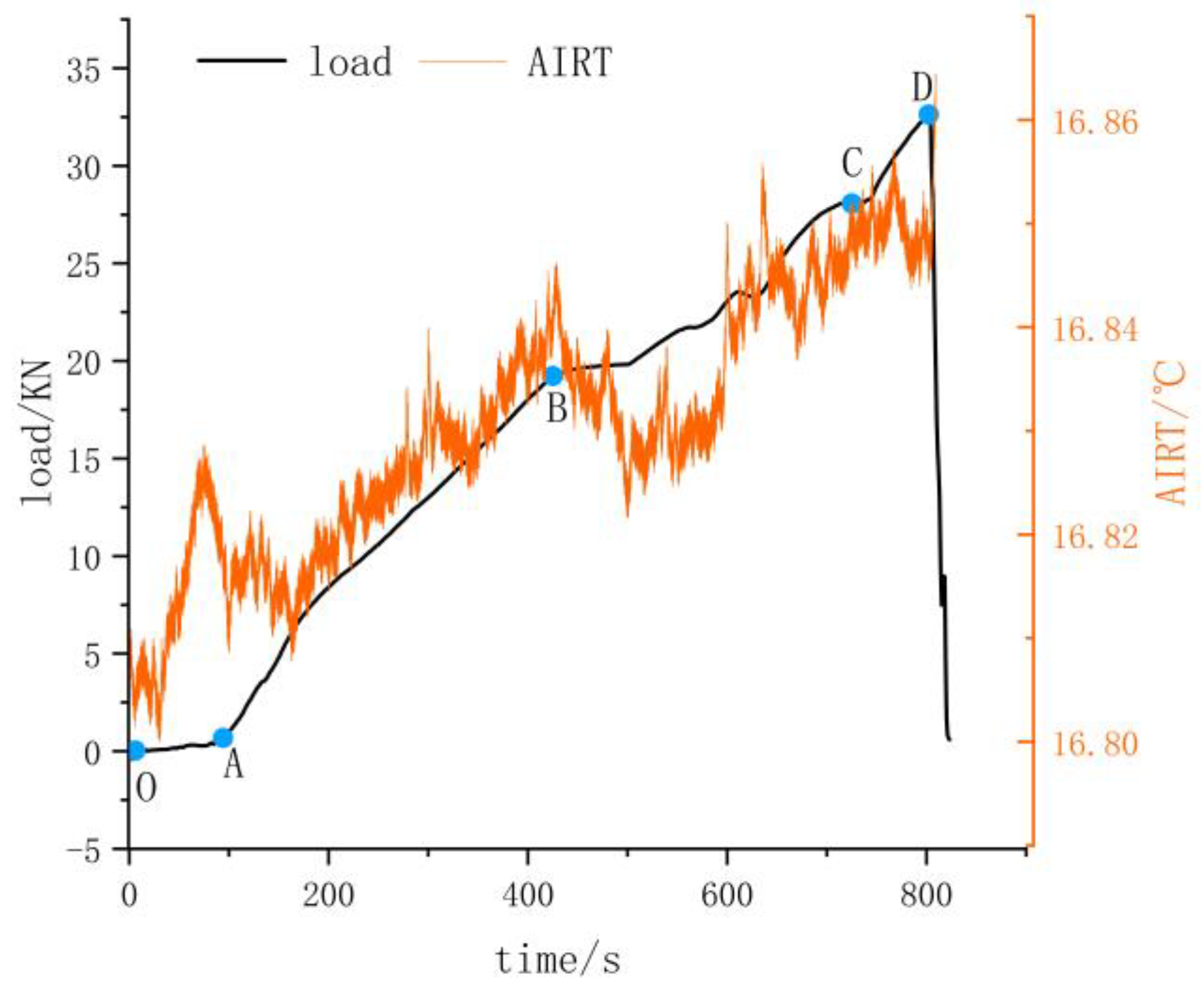
There was a correlation between AIRT and stress during the uniaxial loading of rocks. Due to the limitation of space, only Sample A was selected for image analysis. Figure 9 shows the AIRT–load time curve without denoising, and Figure 10 shows the AIRT–load time curve after algorithm noise reduction.

It can be seen from the figures that AIRT during the loading process was generally increasing before the damage of this specimen. At the early stage of loading (OA stage), the sample was in the pressure-dense stage, when the stress increased more slowly with time and the curve shows a concave form, at which time the AIRT gradually increased over time, and the temperature increased.

At the time of loading to the elastic phase (AB stage), when AIRT was positively correlated with stress growth, the temperature rises due to the thermoelastic effect. When loading to point C (BC stage), at this point in the crack expander the AIRT increase became slower and there was a small, a sudden drop has occurred. In the CD stage, the AIRT appeared to increase; when loaded to point D, the specimen underwent a significant stress drop at 801 s and the AIRT underwent a transient, abrupt change.

In comparing Figure 9 and Figure 10, it is clear that the fluctuations of AIRT data are smoother after the noise reduction process.

For further comparative analysis the AIRT data of the samples were fitted.

The fitting functions for samples are as follows. The degree of fitting of the formula is shown in

Table 3. Degree of fitting of the AIRT formula.

Sample	Degree of Fitting of the Formula
	Before Denoising	After Denoising
A	0.8482	0.9746
B	0.7801	0.7838
C	0.8239	0.8255
D	0.9065	0.9110

.

For Sample A, the AIRT fitting relation before denoising is:

f(x) = 16.805 + 5.1781*10⁻⁶*x + 1.8152*10⁻¹⁰*x² − 7.41*10⁻¹⁴*x³ + 4.2735*10⁻¹⁸*x⁴.

The AIRT fitting relation after denoising is:

f(x) = 16.805 + 5.2049*10⁻⁶*x + 1.4219*10⁻¹⁰*x² − 7.2776*10⁻¹⁴*x³ + 4.2143*10⁻¹⁸*x⁴.

For Sample B, the AIRT fitting relation before denoising is:

f(x) = 16.799 − 1.4273*10⁻⁷*x + 1.3888*10⁻⁹*x² − 2.0379*10⁻¹³*x³ + 8.7585*10⁻¹⁸*x⁴.

For Sample C, the AIRT fitting relation before denoising is:

f(x) = 16.807 + 1.0547*10⁻⁶*x + 9.2707*10⁻¹⁰*x² − 1.3595*10⁻¹³*x³ + 5.973*10⁻¹⁸*x⁴.

The AIRT fitting relation after denoising is:

f(x) = 16.807 + 1.1616*10⁻⁶*x + 8.9461*10⁻¹⁰*x² − 1.3176*10⁻¹³*x³ + 5.8085*10⁻¹⁸*x⁴.

For Sample D, the AIRT fitting relation before denoising is:

f(x) = 16.820 + 1.959*10⁻⁶*x + 1.1912*10⁻⁹*x² − 1.7995*10⁻¹³*x³ + 8.0367*10⁻¹⁸*x⁴.

The AIRT fitting relation after denoising is:

f(x) = 16.822 + 1.9166*10⁻⁶*x + 1.2517*10⁻⁹*x² − 1.8863*10⁻¹³*x³ + 8.4190*10⁻¹⁸*x⁴.

From the above fitting data of four samples, it can be seen that the fluctuation trend of AIRT was more concentrated after denoising.

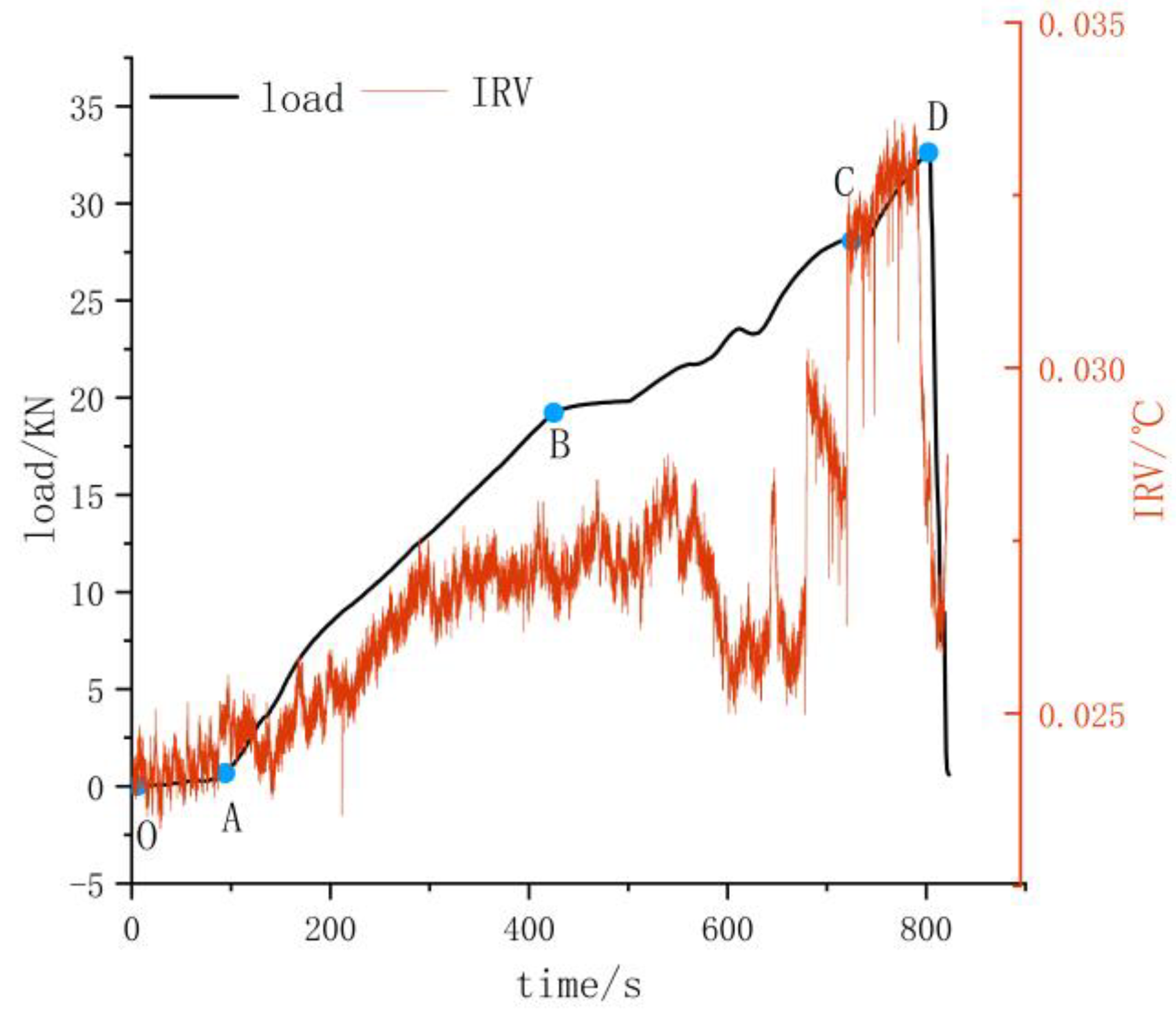
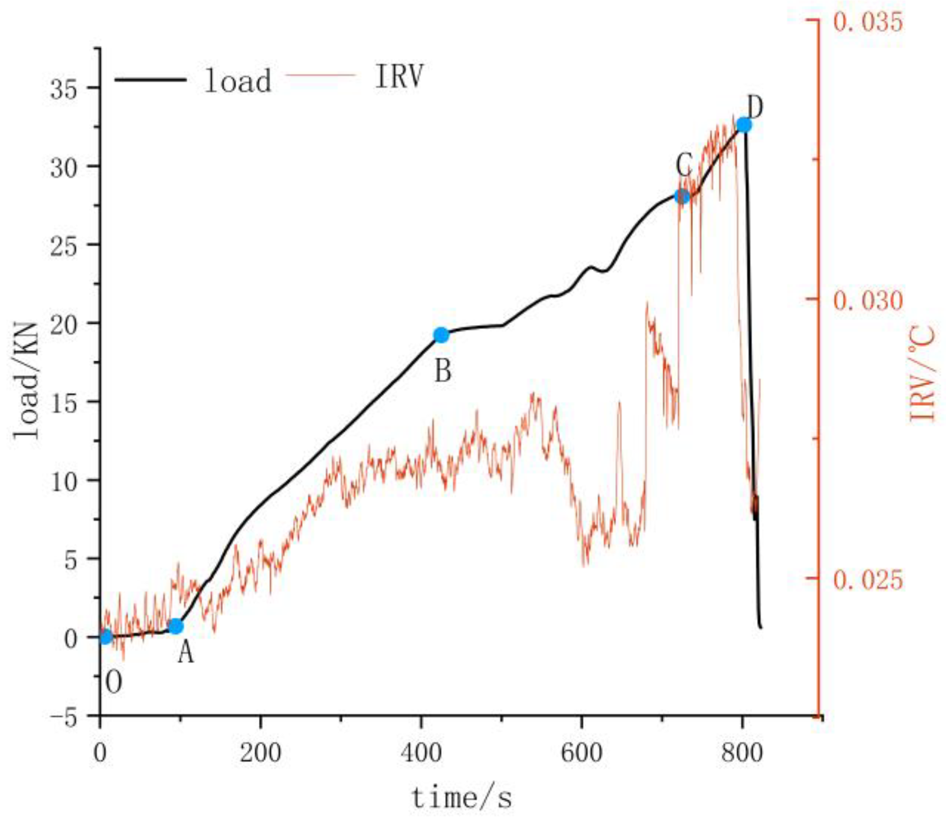
5.4. Indicator of IRV

There was a correlation between IRV and stress during the uniaxial loading of rocks. Due to the limitation of space, only Sample A was selected for image analysis. Figure 11 shows the IRV–load time curve without the denoising process, and Figure 12 shows the IRV–load time curve after the algorithm noise reduction. It can be seen from the figure that the IRV during loading was generally increasing before the damage of this specimen.

At the early stage of loading (OA stage), the sample was in the compression-density stage, when the stress increased more slowly with time and the curve shows a downward concave form, and the IRV gradually increased with time. At loading to the elastic phase (AB stage), when IRV was positively correlated with stress growth, the temperature increased under thermoelastic effects. When loading to point C (BC stage), at this point in the crack expander the IRV increase became slower and there was a small, sudden drop. In the CD section there was an increase in IRV, and when loaded to point D, the specimen underwent a significant stress drop at 789.51 s and a sudden and instantaneous change in IRV. Comparison of Figure 11 and Figure 12 shows clearly that the fluctuations of IRV data are smoother after the noise reduction process.

For further comparative analysis, the IRV data of the samples were fitted.

The fitting functions for the samples are as follows. The degree of fitting of the formula is shown in

Table 4. Degree of fitting of the IRV formula.

Sample	Degree of Fitting of the Formula
	Before Denoising	After Denoising
A	0.9646	0.9746
B	0.5927	0.6087
C	0.8671	0.8990
D	0.9646	0.9751

.

For Sample A, the IRV fitting relation before denoising is:

f(x) = 195.54 − 1.0366*10⁻⁷*x + 2.0589*10⁻¹⁰*x² − 2.7678*10⁻¹⁴*x³ + 1.3168*10⁻¹⁸*x⁴.

The IRV fitting relation after denoising is:

f(x) = 195.54 − 1.0366*10⁻⁷*x + 3.1149*10⁻¹⁰*x² − 3.179*10⁻¹⁴*x³ + 1.8645*10⁻¹⁸*x⁴.

For Sample B, the IRV fitting relation before denoising is:

f(x) = 162.69 − 2.1972*10⁻⁷*x − 5.8093*10⁻¹²*x² + 3.3799*10⁻¹⁵*x³ − 1.0014*10⁻¹⁹*x⁴.

The IRV fitting relation after denoising is:

f(x) = 162.70 − 2.212*10⁻⁷*x − 5.1172*10⁻¹²*x² + 3.2724*10⁻¹⁵*x³ − 9.5187*10⁻²⁰*x⁴.

For Sample C, the IRV fitting relation before denoising is:

f(x) = 180.03 − 4.0661*10⁻⁷*x + 1.8586*10⁻¹⁰*x² − 2.3537*10⁻¹⁴*x³ + 1.0205*10⁻¹⁸*x⁴.

The IRV fitting relation after denoising is:

f(x) = 180.02 − 4.0505*10⁻⁷*x + 1.8520*10⁻¹⁰*x² − 2.3444*10⁻¹⁴*x³ + 1.0162*10⁻¹⁸*x⁴.

For Sample D, the IRV fitting relation before denoising is:

f(x) = 192.95 − 3.1691*10⁻⁷*x + 2.5371*10⁻¹⁰*x² − 3.3*10⁻¹⁴*x³ + 1.5070*10⁻¹⁸*x⁴.

The IRV fitting relation after denoising is:

f(x) = 192.94 − 3.1536*10⁻⁷*x + 2.5287*10⁻¹⁰*x² − 3.287*10⁻¹⁴*x³ + 1.5007*10⁻¹⁸*x⁴.

From the above fitting data of four samples, it can be seen that the fluctuation trend of IRV is more concentrated after denoising.

6. Conclusions

In order to eliminate the influence of noise on infrared radiation, a multi-band pseudo-emissivity algorithm is proposed in this paper. We carried out an infrared monitoring experiment of rock samples under uniaxial compression. During the experiment, the infrared radiation during the loading period was observed, and the infrared characteristic indexes before and after denoising were compared. The following conclusions are drawn.

Based on the basic theory of infrared radiation, the infrared temperature measurement was separated from the emissivity of the measured object, and a three-band infrared temperature measurement vector group without emissivity was constructed to solve the influence of emissivity noise of the object. The multi-band algorithm can measure the temperature without obtaining the emissivity of the measured object. By constructing three vector groups to solve the problem, the actual temperature can be obtained according to the infrared thermal image temperature and the ambient temperature (in the case of unknown emissivity), which solves the problem in the observation process.

During rock loading and damage, abnormal high-temperature areas appeared in infrared images. The location of the high-temperature belt basically corresponded to the actual fault location of the sample. In the noise-reduced infrared image, the abnormally high temperature region gradually appears from the loading, and the high temperature region becomes more and more obvious until the specimen ruptures.

In the process of loading, local stress can occur easily in rock samples, resulting in local fracture and thus leading to stress drop. In addition, local cracks in a sample may cause sudden changes in MIRT, AIRT and IRV in the infrared temperature field. The MIRT, AIRT and IRV indexes after noise reduction algorithm were more accurate.

The infrared images reflected the spatial distribution characteristics of temperature during the loading process of coal and rock, and the infrared radiation temperature field indexes (MIRT, AIRT, IRV) can be regarded as feedback signals of rock failure, and areearly-warning precursors of coal and rock damage. Since the denoised infrared radiation temperature field indexes (MIRT, AIRT, IRV) were more accurate, this suggests that the instability of coal and rock during mining provides more accurate precursor information. The denoised infrared radiation temperature field index could help to accurately identify fracture areas in mine rocks. The research results lay the theoretical and experimental basis for the use of infrared radiation to monitor the stability of mine rock mass, and to promote the monitoring and early warning of rock failure.

In conclusion, by using the denoising algorithm proposed in this paper, the infrared radiation information and characteristics of uniaxial compressed rock can be obtained without the influence of sample emissivity. In our experiments, the infrared radiation index of the denoised sample was closer to the stress, and the infrared radiation fluctuation of the coal sample was more obvious when the stress changed suddenly. Combined with infrared thermal images, the results indicate that there are obvious infrared radiation precursors before rock fracture.

In future, we will further study the relationship between the fracture mechanism and the infrared radiation image during the loading process of coal and rock, combined with the acoustic emission measurement or CT scanning measurement The infrared radiation image will be combined with mesoscopic damage mechanics to analyze the failure state and the rock. The internal relationship between fractures and the relationship between infrared radiation temperature and crack propagation will be quantitatively analyzed.

References

- Shen, R.; Li, H.R.; Wang, E.Y.; Chen, T.Q.; Li, T.X.; Tian, H.; Hou, Z.H. Infrared radiation characteristics and fracture precursor information extraction of loaded sandstone samples with varying moisture contents. Int. J. Rock Mech. Min. Sci. 2020, 130, 104344. [Google Scholar] [CrossRef]
- Cao, K.W.; Ma, L.Q.; Wu, Y.; Spearing, A.J.S.; Naseer, M.; Hussain, S.; Faheem, U. Statistical damage model for dry and saturated rock under uniaxial loading based on infrared radiation for possible stress prediction. Eng. Fract. Mech. 2022, 260, 108134. [Google Scholar] [CrossRef]
- Sun, X.; Xu, H.; He, M.; Zhang, F. Experimental investigation of the occurrence of rockburst in a rock specimen through infrared thermography and acoustic emission. Int. J. Rock Mech. Min. Sci. 2017, 100, 250–259. [Google Scholar] [CrossRef]
- Pappalardo, G.; Mineo, S.; Zampelli, S.P.; Cubito, A.; Calcaterra, D. Infrared thermography proposed for the estimation of the Cooling Rate Index in the remote survey of rock masses. Int. J. Rock Mech. Min. Sci. 2016, 83, 182–196. [Google Scholar] [CrossRef]
- Mineo, S.; Pappalardo, G.; Rapisarda, F.; Cubito, A.; Maria, G. Integrated geostructural, seismic and infrared thermography surveys for the study of an unstable rock slope in the Peloritani Chain (NE Sicily). Eng. Geol. 2015, 195, 225–235. [Google Scholar] [CrossRef]
- Cheng, X.; Fu, T.; Fan, X. The principle of primary spectrum pyrometry. Sci. China Ser. G Phys. Mech. Astron. 2005, 48, 142–149. [Google Scholar] [CrossRef]
- Fu, T.R.; Cheng, X.F.; Zhong, M.H. The application analyses for primary spectrum pyrometer. Sci. China Ser. G Phys. Mech. Astron. 2007, 50, 753–765. [Google Scholar] [CrossRef]
- Shen, J.; Zhang, Y.; Xing, T. The study on the measurement accuracy of non-steady state temperature field under different emissivity using infrared thermal image. Infrared Phys. Technol. 2018, 94, 207–213. [Google Scholar] [CrossRef]
- He, M.C.; Fei, Z.; Yu, Z.; Shuai, D.; Lei, G. Feature evolution of dominant frequency components in acoustic emissions of instantaneous strain-type granitic rockburst simulation tests. Rock Soil Mech. 2015, 36, 1–8. [Google Scholar]
- Zhou, X.P.; Qian, Q.H.; Yang, H.Q. Rock burst of deep circular tunnels surrounded by weakened rock mass with cracks. Theor. Appl. Fract. Mech. 2011, 56, 79–88. [Google Scholar] [CrossRef]
- Feng, X.T.; Young, R.P.; Reyes-Montes, J.M.; Aydan, O.; Ishida, T.; Liu, J.P.; Liu, H.J. ISRM suggested method for in situ acoustic emission monitoring of the fracturing process in rock masses. Rock Mech. Rock Eng. 2019, 52, 1395–1414. [Google Scholar] [CrossRef]
- Ishida, T.; Labuz, J.F.; Manthei, G.; Meredith, P.; Nasseri, M.; Shin, K.; Yokoyama, T.; Zang, A. ISRM suggested method for laboratory acoustic emission monitoring. Rock Mech. Rock Eng. 2017, 50, 665–674. [Google Scholar] [CrossRef]
- Zhang, K.; Liu, X.; Chen, Y.; Cheng, H. Quantitative description of infrared radiation characteristics of preflawed sandstone during fracturing process. J. Rock Mech. Geotech. Eng. 2021, 13, 131–142. [Google Scholar] [CrossRef]
- Shi, D.P.; Xie, C.Y.; Xiong, L.C. Changes in the Structures and Directions of Rock Excavation Research from 1999 to 2020: A Bibliometric Study. Adv. Civ. Eng. 2021, 2021, 1–8. [Google Scholar] [CrossRef]
- Cai, J.; Xie, C.Y.; Zhiru, H. Ecological evaluation of heavy metal pollution in the soil of Pb-Zn mines. Ecotoxicology 2022, 31, 259–270. [Google Scholar] [CrossRef]
- Deng, M.; Geng, N.; Cui, C.; Zhi, Y.Q.; Fan, Z.F.; Ji, Q.Q. The study on the variation of thermal state of rocks caused by the variation of stress state of rocks. Earthq. Res. China 1997, 13, 179–185. [Google Scholar]
- Wu, L.X.; Cui, C.Y.; Geng, N.G.; Wang, J.Z. Remote sensing rock mechanics (RSRM) and associated experimental studies. Int. J. Rock Mech. Min. Sci. 2000, 37, 879–888. [Google Scholar] [CrossRef]
- Wu, L.X.; Liu, S.J.; Wu, Y.H.; Wang, C.Y. Precursors for rock fracturing and failure-Part I: IRR image abnormalities. Int. J. Rock Mech. Min. Sci. 2006, 43, 473–482. [Google Scholar] [CrossRef]
- Wu, L.X.; Liu, S.J.; Wu, Y.H.; Wang, C.Y. Precursors for rock fracturing and failure-Part II: IRR T-Curve abnormalities. Int. J. Rock Mech. Min. Sci. 2006, 43, 483–493. [Google Scholar] [CrossRef]
- Ma, L.Q.; Sun, H.; Zhang, Y.; Hu, H.; Zhang, C. The role of stress in controlling infrared radiation during coal and rock failure. Strain 2018, 54, e12295. [Google Scholar] [CrossRef]
- Ma, L.Q.; Sun, H.; Zhang, Y.; Zhou, T.; Li, K.; Guo, J. Characteristics of infrared radiation of coal specimens under uniaxial loading. Rock Mech. Rock Eng. 2016, 49, 1567–1572. [Google Scholar] [CrossRef]
- Ma, L.Q.; Sun, H. Spatial-temporal infrared radiation precursors of coal failure under uniaxial compressive loading. Infrared Phys. Technol. 2018, 93, 144–153. [Google Scholar] [CrossRef]
- Freund, F.T. Rocks that crackle and sparkle and glow: Strange pre-earthquake phenomena. J. Sci. Explor. 2003, 17, 37–71. [Google Scholar]
- Luong, M.P. Infrared thermographic observations of rock failure. Compr. Rock Eng. 1993, 26, 715–730. [Google Scholar]
- Grinzato, E.; Marinetti, S.; Bison, P.G.; Concas, M.; Fais, S. Comparison of ultrasonic velocity and IR thermography for the characterisation of stones. Infrared Phys. Technol. 2004, 46, 63–68. [Google Scholar] [CrossRef]
- Yang, H.; Liu, B.; Karekal, S. Experimental investigation on infrared radiation features of fracturing process in jointed rock under concentrated load. Int. J. Rock Mech. Min. Sci. 2021, 139, 104619. [Google Scholar] [CrossRef]
- Cao, K.; Ma, L.; Wu, Y.; Khan, N.M.; Yang, J. Using the characteristics of infrared radiation during the process of strain energy evolution in saturated rock as a precursor for violent failure. Infrared Phys. Technol. 2020, 109, 103406. [Google Scholar] [CrossRef]
- Wang, S.; Li, D.; Li, C.; Zhang, C.; Zhang, Y. Thermal radiation characteristics of stress evolution of a circular tunnel excavation under different confining pressure. Tunn. Undergr. Space Technol. 2018, 78, 76–83. [Google Scholar] [CrossRef]
- Deng, M.D.; Cui, C.Y.; Geng, N.G.; Zhi, Y.Q. Study of the infrared waveband radiation characteristics of rocks. J. Infrared Millim. Waves 1994, 13, 425–430. [Google Scholar]
- Zhang, X.Q.; Zou, J.X. Research on collaborative control technology of coal spontaneous combustion and gas coupling disaster in goaf based on dynamic isolation. Fuel 2022, 321, 124123. [Google Scholar] [CrossRef]
- Fan, S.; Song, Z.; Xu, T.; Zhang, Y. Investigation of the microstructure damage and mechanical properties evolution of limestone subjected to high-pressure water. Constr. Build. Mater. 2022, 316, 125871. [Google Scholar] [CrossRef]
- Sun, H.; Liu, X.L.; Zhang, S.G.; Nawnit, K. Experimental investigation of acoustic emission and infrared radiation thermography of dynamic fracturing process of hard rock pillar in extremely steep and thick coal seams. Eng. Fract. Mech. 2020, 226, 106845. [Google Scholar] [CrossRef]
- Li, Z.; Yin, S.; Niu, Y.; Cheng, F.Q.; Liu, S.J.; Sun, Y.H. Experimental study on the infrared thermal imaging of a coal fracture under the coupled effects of stress and gas. J. Nat. Gas Sci. Eng. 2018, 55, 444–451. [Google Scholar] [CrossRef]
- Sun, H.; Konietzky, H.; Wang, F.; Herbst, M. Some Thoughts about Infrared Radiation Response Characteristics during Loading of Coal and Sandstone Samples. Res. Sq. 2022. [Google Scholar] [CrossRef]
- Yang, Z.; Zhang, S.C.; Yang, L. Altering Spectrum Method in Temperature Measurement Using Infrared Imager in Complex Background Environment. In Advanced Materials Research; Trans Tech Publications Ltd.: Wollerau, Switzerland, 2012; Volume 479, pp. 348–351. [Google Scholar]
- Sun, H.; Ma, L.Q.; Adeleke, N.; Zhang, Y. Background thermal noise correction methodology for average infrared radiation temperature of coal under uniaxial loading. Infrared Phys. Technol. 2017, 81, 157–165. [Google Scholar] [CrossRef]
- Yang, Z.; Yang, L.; Zhang, S. Infrared temperature measurement technology on Lambertian based on the dual temperature and dual-band method. J. Eng. Thermophys. 2013, 34, 2132–2135. [Google Scholar]
- Li, Z.J.; Shi, D.P.; Wu, C.; Wang, X.L. Infrared thermography for prediction of spontaneous combustion of sulfide ores. Trans. Nonferrous Met. Soc. China 2012, 22, 3095–3102. [Google Scholar] [CrossRef]
- Shi, D.; Wu, C.; Li, Z.; Nan, J.; Pan, W. Optimized tri-wavelength infrared temperature measurement introducing dimensionless model and bending coefficient. Infrared Laser Eng. 2015, 45, 0204006. [Google Scholar]
- Shi, D.; Wu, C.; Li, Z.; Pan, W. Analysis of the influence of infrared temperature measurement based on reflected temperature compensation and incidence temperature compensation. Infrared Laser Eng. 2015, 44, 2321. [Google Scholar]
- Chen, C.; Shi, D.P. The Atmospheric Environment Effects of the COVID-19 Pandemic: A Metrological Study. Int. J. Environ. Res. Public Health 2022, 9, 11111. [Google Scholar] [CrossRef] [PubMed]
- Liu, S.J.; Wei, J.L.; Huang, J.W.; Wu, L.X.; Zhang, Y.B.; Tian, B.Z. Quantitative analysis methods of infrared radiation temperature field variation in rock loading process. Chin. J. Rock Mech. Eng. 2015, 34, 2968–2976. [Google Scholar]
- Wang, H.; Yang, T.H.; Liu, H.L.; Zhao, Y. Deformation and acoustic emission characteristics of dry and saturated sand under cyclic loading and unloading process. J. Northeast. Univ. (Nat. Sci.) 2016, 37, 1161. [Google Scholar]
- Gong, W.L.; Gong, Y.X.; Long, A.F. Multi-filter analysis of infrared images from the excavation experiment in horizontally stratified rocks. Infrared Phys. Technol. 2013, 56, 57–68. [Google Scholar] [CrossRef]
- Xie, C.Y.; Nguyen, H.; Bui, X.; Nguyen, V.T.; Zhou, J. Predicting roof displacement of roadways in underground coal mines using adaptive neuro-fuzzy inference system optimized by various physics-based optimization algorithms. J. Rock Mech. Geotech. Eng. 2021, 13, 1452–1465. [Google Scholar] [CrossRef]
- Xie, C.Y.; Nguyen, H.; Choi, Y.; Armaghani, D.J. Optimized functional linked neural network for predicting diaphragm wall deflection induced by braced excavations in clays. Geosci. Front. 2022, 13, 101313. [Google Scholar] [CrossRef]
- Amann, F.; Button, E.A.; Evans, K.F.; Gischig, V.S. Experimental study of the brittle behavior of clay shale in rapid unconfined compression. Rock Mech. Rock Eng. 2011, 44, 415–430. [Google Scholar] [CrossRef] [Green Version]
- Lou, Q.; He, X. Experimental study on infrared radiation temperature field of concrete under uniaxial compression. Infrared Phys. Technol. 2019, 90, 20–30. [Google Scholar] [CrossRef]
- Yao, Q.; Chen, T.; Ju, M.; Liang, S.; Liu, Y.; Li, X. Effects of water intrusion on mechanical properties of and crack propagation in coal. Rock Mech. Rock Eng. 2016, 49, 4699–4709. [Google Scholar] [CrossRef]
- Chen, T.; Yao, Q.L.; Du, M.; Zhou, C.G.; Zhang, B. Experimental research of effect of water intrusion times on crack propagation in coal. Chin. J. Rock Mech. Eng A 2016, 2, 3756–3762. [Google Scholar]
Figure 1.
Schematic diagram of the experiment.
Figure 2.
Method for processing infrared images.
Figure 3.
IRT of Sample A: (a) 102 s, (b) 200 s, (c) 576 s, (d) 800 s, (e) 963 s.
Figure 4.
Noise reduction IRT of Sample A: (a) 102 s, (b) 200 s, (c) 576 s, (d) 800 s, (e) 963 s.
Figure 5.
Three-dimensional cloud map of Sample A at 800 s (without denoising).
Figure 6.
Three-dimensional cloud map of Sample A at 800 s (after denoising).
Figure 7.
Load–time curves and MIRT–time curves of Sample A (without denoising).
Figure 8.
Load–time curves and MIRT–time curves of Sample A (after denoising).
Figure 9.
Load–time curves and AIRT–time curves of sample A (without denoising).
Figure 10.
Load–time curves and AIRT–time curves for Sample A (after denoising).
Figure 11.
Load–time curves and IRV–time curves of Sample A (without denoising).
Figure 12.
Load–time curves and IRV–time curves of Sample A (after denoising).