
Urban Heat Island Mitigation through Planned Simulation
by
 , and
, and
Paul Eduardo Vásquez-Álvarez
1,*, 
Carlos Flores-Vázquez
2 ,
,
Juan-Carlos Cobos-Torres
3 and
Sandra Lucía Cobos-Mora
4,5,* 1
Academic Unit of Postgraduate, Master’s Program in Construction, Catholic University of Cuenca, Cuenca 010111, Ecuador
2
Academic Unit of Postgraduate, Electrical Engineering Career, Visible Radiation and Prototyping Research Group GIRVyP, Research, Innovation and Technology Transfer Center (CIITT), Catholic University of Cuenca, Cuenca 010111, Ecuador
3
Academic Unit of Postgraduate, Electrical Engineering Career, Visible Radiation and Prototyping Research Group GIRVyP, Embedded Systems and Artificial Vision in Architectural, Agricultural, Environmental and Automatic Sciences Research Group (SEVA4CA), Catholic University of Cuenca, Cuenca 010111, Ecuador
4
Academic Unit of Postgraduate, Research, Innovation and Technology Transfer Center (CIITT), Civil Engineering Career, Urban and Earth Data Science Research Group, City, Environment and Technology Research Group, Catholic University of Cuenca, Cuenca 010111, Ecuador
5
Department of Physical Geography and Regional Geographical Analysis, University of Sevilla, 41004 Sevilla, Spain
*
Authors to whom correspondence should be addressed.
Sustainability 2022, 14(14), 8612; https://doi.org/10.3390/su14148612
Submission received: 18 January 2022
/
Revised: 20 June 2022
/
Accepted: 23 June 2022
/
Published: 14 July 2022
(This article belongs to the Topic Sustainable Built Environment)
Abstract
:The urban heat island (UHI) phenomenon is caused by the anthropic alteration of the natural environment by urban expansion, its impermeable surfaces, and anthropic activities. In addition, urban morphology can also contribute to the increase in temperature in cities. The UHI effect can be described as an urban climate that is generally characterized by higher temperatures in densely built-up areas compared to surrounding areas. This effect impacts the environmental stress of the city and directly affects the health and quality of life of its inhabitants. Therefore, it is necessary to allocate resources to understand the UHI mechanism in cities in order to propose appropriate mitigation measures that will reduce energy consumption and improve living conditions. In this context, this research was aimed at analyzing the behavior of urban heat islands by replacing asphalt with cool paving materials (concrete) in roadways. Through computer simulations, using the ENVI-met software, the thermal variations of urban heat islands were examined. The city of Cuenca (Ecuador) was selected as the study area. The day of the analysis was 22 January 2020, which was recorded as the warmest day of the year, registering an average temperature of 16 °C. The findings of this research evidenced that, by replacing asphalt pavements with concrete pavements in the analyzed zones, land surface temperature (LST) could be reduced by 8 °C and the global LST of the studied areas could be reduced by approximately 3 °C. Consequently, the mean air temperature of the study areas reflected a decrease of up to 0.83 °C.
1. Introduction
The UHI is a climatic phenomenon that occurs when temperatures in urban areas tend to be higher than in their surrounding or rural areas [1]. UHIs can be detected in several cities around the world, e.g., Lucknow City [2], India, Nanchang City; (China) [3], Singapore [4], Madrid [5], Colombo [6], Wuhan [7], Melbourne [8], Karaj [9], and Sydney [10]. One of the main causes of UHIs is the alteration of the Earth’s surface through anthropogenic activities [11], such as the replacement of vegetation cover with impervious construction materials used in city infrastructure [12]. However, there are other factors for this effect, including the spatial contiguity of urban development [13], spatiotemporal patterns [14], and climatic conditions [15].
It is estimated that by 2030, approximately 61% of the global population will be living in high-density urban areas [16]. The urbanization process is closely associated with land-use and land-cover changes [17]; as a consequence of this fact, cities’ temperatures are expected to gradually increase in accordance with the UHI effect. In theory, average UHI intensity varies from 2 to 4 °C, and the maximum intensity ranges from 7 to 14 °C [8]. These values depend on the location of a city, its topographic characteristics, and its elements, such as roads, vegetation cover, and building structures. For urban planners, the increasing temperatures in cities emphasize the need to rethink development models to shift their primary focus towards sustainability [18] and energy efficiency [19], especially because this warming effect has critical impacts on health, wellbeing, human comfort, and the local atmosphere. It includes significant environmental stress increases on the planet [20], increases in morbidity and mortality rates [12], increases in peak electricity demand [21], and air quality degradation via the presence of ozone and nitrogen oxide [22].
The extent of a UHI is usually estimated through air temperature or LST. Air temperature is usually determined through meteorological data from nearby stations, and satellite or airborne sensor data are used to determine LST. The major limitation of analyzing a UHI through air temperature is the availability and distribution of meteorological stations. On the other hand, although LST is an indirect measure of a UHI, it does not require the availability of meteorological stations in the study areas and allows for the explicit analysis of a determined UHI surface [23].
Road infrastructure is the urban component with the largest horizontal surface area (approximately 20%) exposed to direct solar radiation [24]. Its material composition is determined by its thermal and optical properties, specifically the albedo (the percentage of radiation reflected by a surface), emissivity, thermal conductivity, diffusivity, and heat capacity [25], which positively or negatively contribute to the UHI effect [26]. This effect is also influenced by local climatic conditions [27]. In this context, asphalt, one of the most popular materials for urban streets, is also one of the main causes of rising temperatures in cities [20] due to its low albedo content and higher radiation absorption, thus increasing the temperature of ambient air and pavement surfaces [28,29].
To mitigate UHI effects, there are some strategies widely discussed in the literature, e.g., increasing the amount of vegetation allowed Maleki and Mahdav [30] to achieve a reduction in the air temperature of up to 3 °C. There is also the use of cool roofs [31]. In this context, Zhang [32] demonstrated a maximum roof surface temperature difference from 2.5 °C to 5.7 °C depending on the season of the year. Another common approach is the use of cool pavements, such as reflective pavements, permeable pavements, the use of phase change materials in the mass of the pavement, the circulation of water in the mass of asphaltic pavements, and the use of photovoltaic pavements [33]. In this respect, Sen et al. [34] demonstrated a decrease in the air temperature of 0.20–0.40 °C, and Kyriakodis et al. [35] demonstrated a reduction of up to 1.5 °C in ambient temperature and 11.5 °C in LST.
Within this context, major Ecuadorian cities are already experiencing gradual increases in temperatures in urban areas [36]. In Cuenca, the UHI effect has been identified due to thermal variations in urban areas ranging from 2 to 5 °C compared to the rural areas of the city [37]. Narváez et al. [24] acknowledged that urban areas with less vegetation cover and a higher percentage of asphalt road surface have increased UHI effects because asphalt has a low albedo and it therefore absorbs solar radiation. Bustamante et al. [38] found that in Cuenca, this phenomenon is most evident in an urban area known as El Vecino, where a meteorology monitoring station is located. The station reports temperatures that are 3.24 °C higher than those reported by a station located in a rural area known as Quingeo.
Cities and their populations are subject to climate change caused by both heat-waves and UHIs, which are two types of heat-related impacts that can combine to generate synergistic impacts and cause negative effects for inhabitants [39]. It is essential to have the means to study local urban climates, especially at the microscale level [40] because this level provides detailed thermal information for a deep understanding of relevant processes, which facilitates the prediction of a particular location’s behavior at a given time and provides control over variables that directly interfere with these measurements [41].
Nowadays, scenario simulations employing techniques and software allow for the study of physical phenomena with great precision. Microscale modeling and simulation studies have proven to be efficient alternatives to mitigating the UHI problem [42,43,44]. There are multiple UHI mitigation strategies involving green roofs, reflective materials, blue infrastructure, vegetation cover, and cool pavements. However, the generated cooling performance may be different within different urban contexts. The comparison of multiple hypothetical scenarios with simulated reality enables researchers to generate timely solutions or measures to mitigate the negative effects of environmental phenomena. In view of this, this research was intended to propose scenarios for mitigating the UHI effect by performing simulations using the ENVI-met software v5.0.0 in which current asphalt materials for road networks were replaced by concrete, which is a type of cool pavement and has a higher albedo coefficient. This allowed for comparisons of surface and air thermal variations through heat maps. For this purpose, three areas located in Cuenca (Barrio Sucre, Monay, and El Vergel) were selected because their roads are mainly composed of asphalt materials (approximately 90%) and they are highly densified residential areas [24]. The number of areas selected for our numerical simulation model was in concordance with the analysis performed by Kyriakodis et al. [35].
2. Materials and Methods
2.1. Study Area
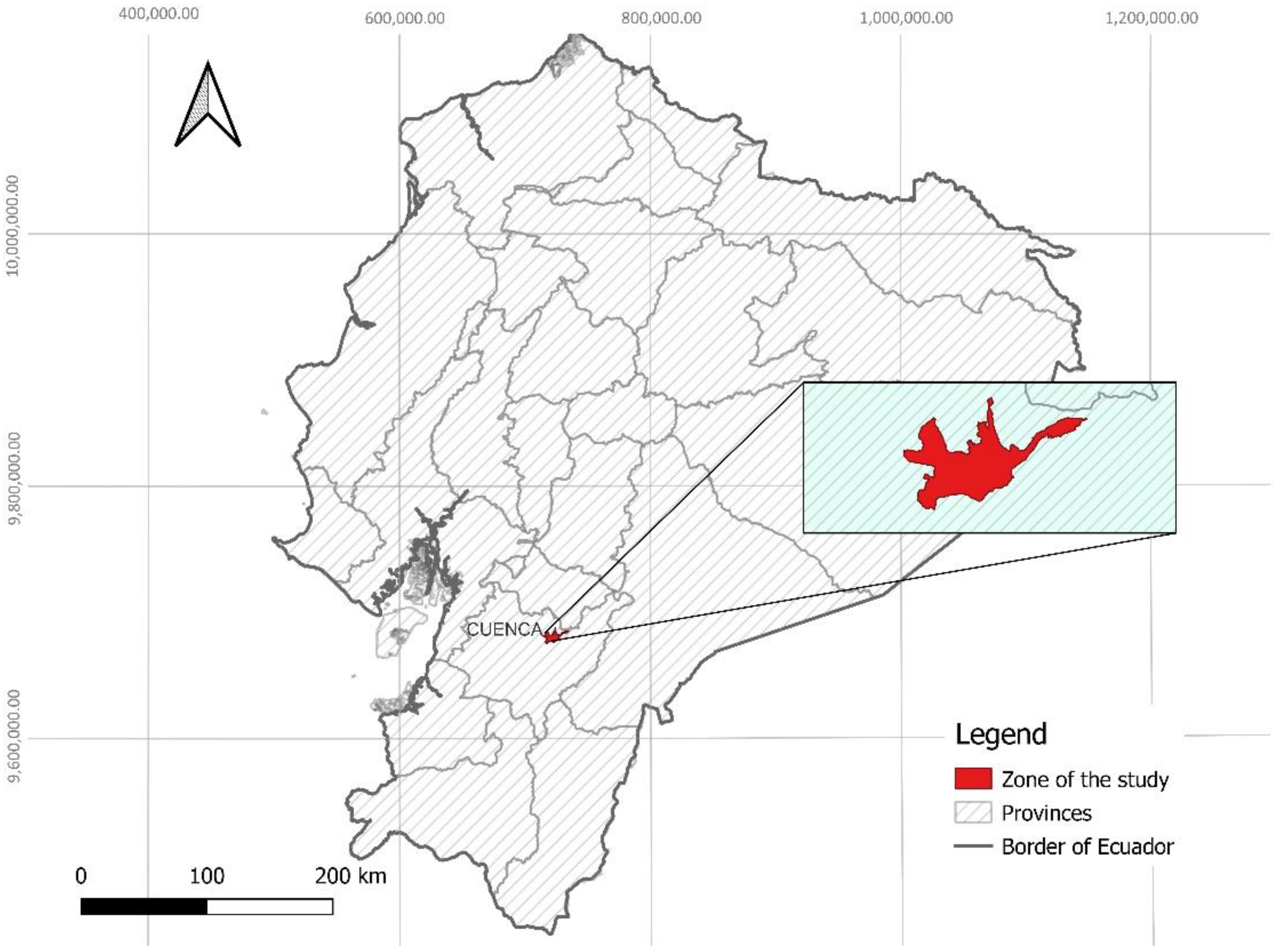
The city of Cuenca (Figure 1), the capital of the province of Azuay, is one of the largest and most populated cities in southern Ecuador. Its urban area is home to about 505,000 people, which represents 71.1% of the inhabitants of Azuay [45]. The annual urban population growth of Cuenca is estimated to be about 120 ha [46]. The city has an urban area of 6923 ha and a rural area of 368,520.11 ha. [47]. Its average altitude is 2550 m.a.s.l; the city is located in an extensive valley in the middle of the Andeans Mountains. Because of these features, the temperature of the city oscillates between 7 and 25 °C. According to the Koppen–Geiger climate classification, Cuenca has a Marnie West Coast Cfb climate [48], with an average annual temperature of 14.7 °C [49].
2.2. Methodology
This research was based on computer simulations of real geospatial models under specific climatic conditions (Table 1). Using simulated scenarios, the UHI effect was analyzed under different conditions (e.g., materials for urban infrastructure and the replacement of asphalt for pavements), as proposed in previous research [50,51,52]. The objective of this simulation was to graphically and statistically determine the behavior of UHIs depending on the materials applied in different scenarios of the analyzed zones. The results helped determine the best measures to mitigate the UHI effect in the study area. The workflow of these simulations is shown in Figure 2.
2.2.1. Study Design
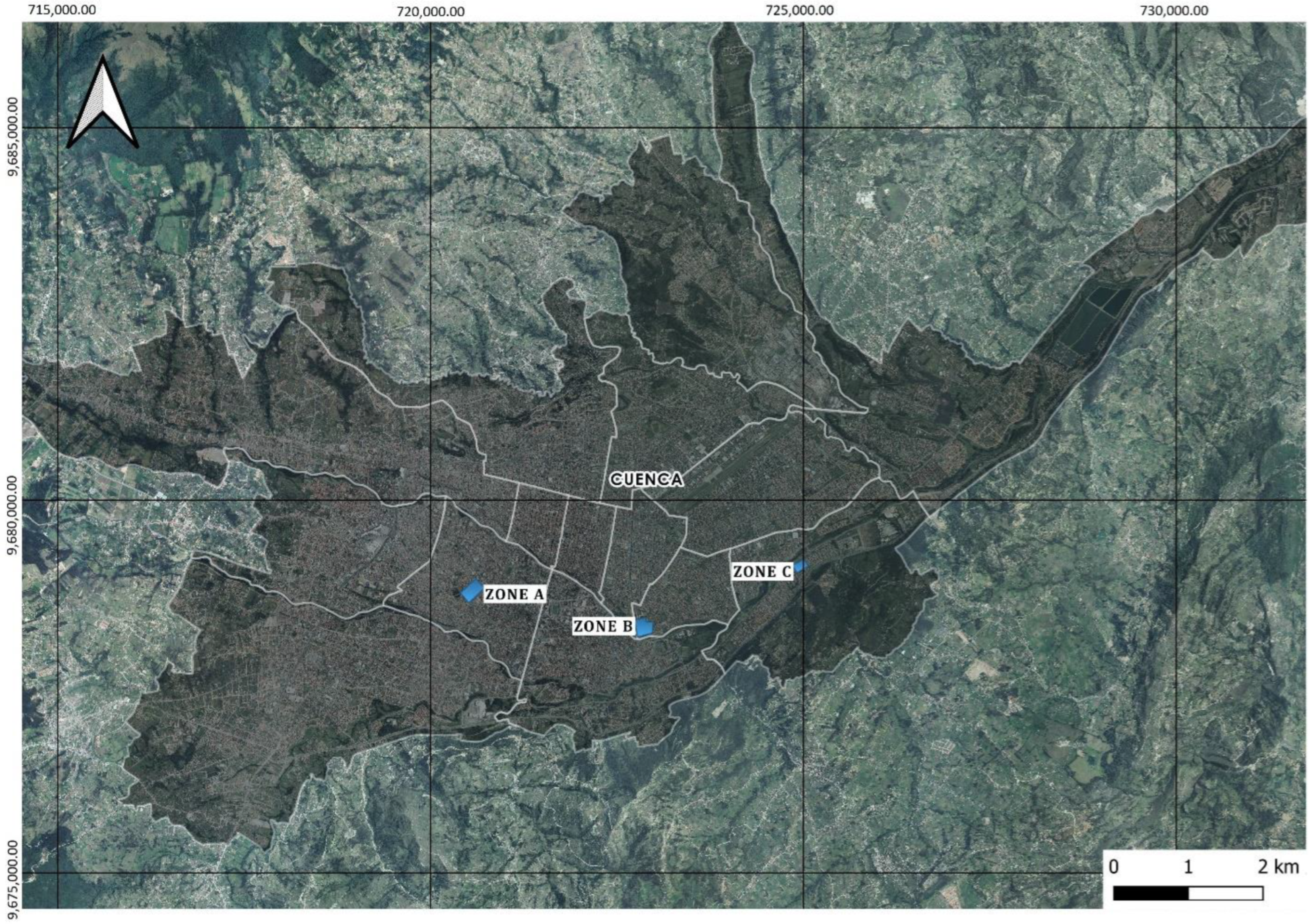
When selecting the urban areas of interest for this study, those with the highest percentages of asphalt in their road network were considered. According to Narváez et al. [24], the Sucre, Cañaribamba, and Monay parishes met said criterion. From each of these three zones, an area with an average surface of 6 ha was selected to create computer-based scenarios. Zone A was located in the center of Sucre, and its analysis area was 200 × 300 m. Zone B was located southwest of Cañaribamba, and its analysis area was 200 × 300 m. Lastly, Zone C was located south of Monay, and its analysis area was 120 × 220 m (Figure 3).
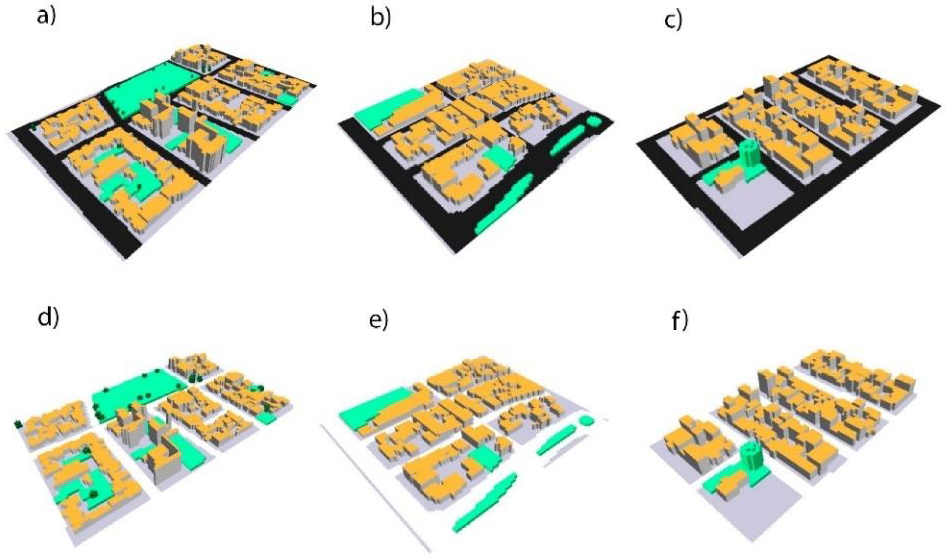
All three-dimensional base scenarios (Figure 4a–c), including roads, buildings, and green surfaces, were digitized with a resolution of 2 m for the horizontal plane and 5 m for the vertical plane (Figure 4). These scenarios demonstrated the current state of the analyzed zones (A, B, and C), while the mitigation scenarios (Figure 4d–f) demonstrated the state of the zones following the substitution of asphalt with concrete.
2.2.2. Weather Inputs
The meteorological parameters used in this research and specified in Table 1 corresponded to those of 22 January 2020, which was the warmest day of 2020 in Cuenca, Ecuador according to the records of the National Aeronautics and Space Administration (NASA). On this day, the average air temperature was 15.03 °C and the maximum temperature was 20 °C. The meteorological parameters were directly obtained from the “Power Data Viewer” platform with the “Power Report” widget from the NASA Langley Research Center (LaRC) POWER Project [53]. These parameters were derived from NASA’s GMAO MERRA-2 assimilation model and GEOS 5.12.4 FP-IT. MERRA-2 is a version of NASA’s Goddard Earth Observing System (GEOS) Data Assimilation System [54]. MERRA-2 is composed of multiple satellites that allow for an approximate resolution of 0.5° × 0.65° around the world [55]. The data were downloaded in the CSV format.
2.2.3. Material Characteristics Input
After structuring three-dimensional geospatial models of the analyzed zones, the thermal characteristics of materials (thermal absorption or albedo) that interact with pre-established meteorological conditions were established. The used characteristics were given by ENVI-met and are shown in Table 2 [56].
2.2.4. Simulations
After establishing the thermophysical characteristics of the materials, digitizing the scenarios, determining the climatic conditions of the zones, and detailing the timing of the simulations, simulations for 12 consecutive hours were established from 06:00 to 18:00 h at one-second intervals on 22 January 2020, following the recommendation of Faragallah et al. [57]. The results of these simulations were represented in heat maps, for which LST and air temperature data were obtained at noon on the day of analysis for each zone of interest.
2.2.5. Data Validation
The validation process of the simulated air temperature model was performed through comparisons between the experimental measurements and the measurements of the predicted results for the same analysis date. The first data were obtained from the Power View Data platform [53] in the CSV format, and the simulation provided the second data. These comparison were conducted using the coefficient of determination (R2) as a quantitative measure for the statistical validation of the models [45]. This coefficient is widely used to validate simulation studies for urban microclimates [58,59,60]. R2 is used to describe the agreement between model forecasts and observed field values, and it represents the proportion of variance between the dependent variables. R2 values can range from 0 to 1 [57], from which it is inferred that models are highly correlated when their R2 values are close to 1.
3. Results
3.1. Surface Temperature
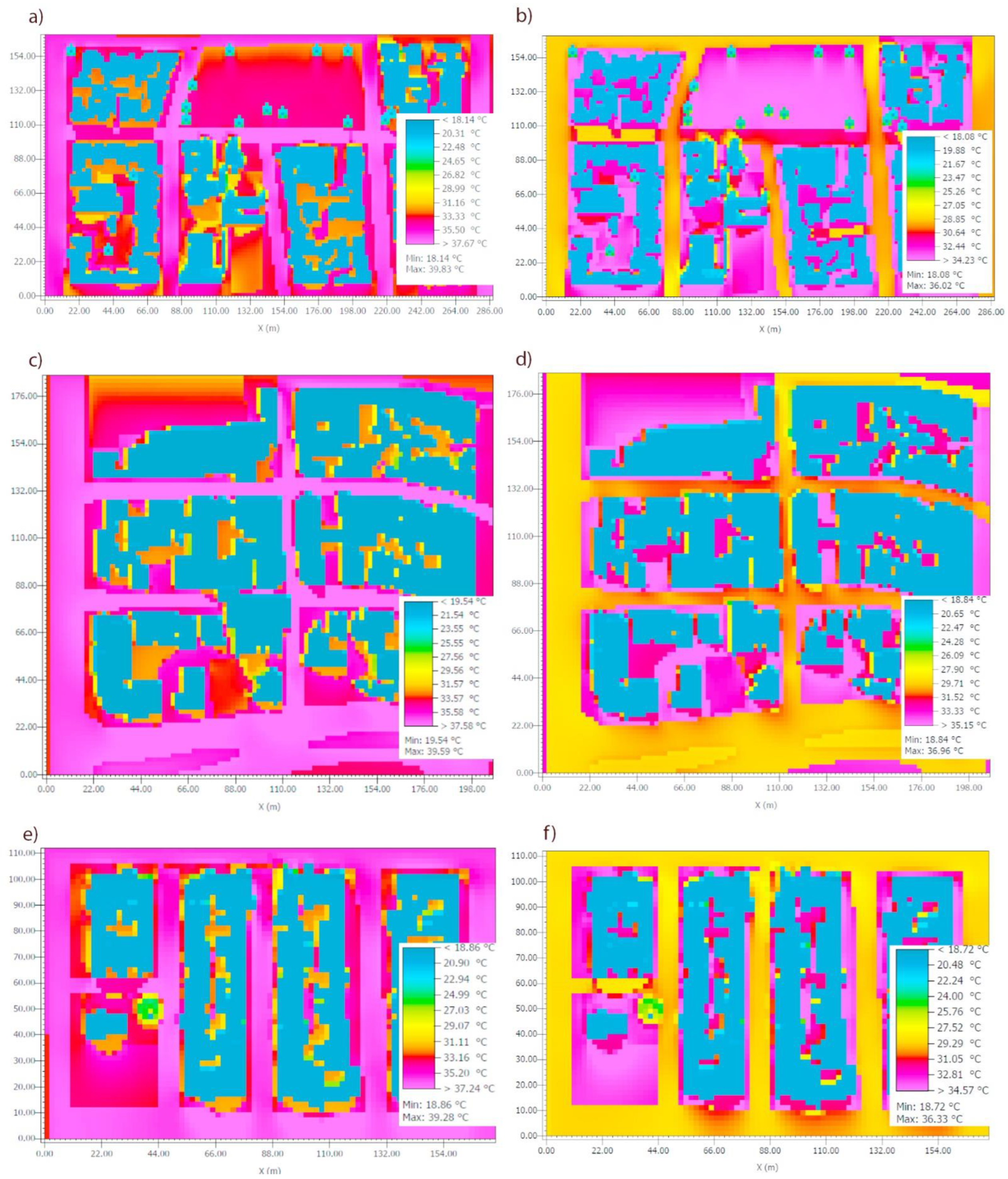
LST maps of base scenarios (Figure 5) showed approximate maximum values of 40 °C and minimum values of 18 °C. On the other hand, in the mitigation scenarios, LST reached a maximum of 36 °C and a minimum of 18 °C. In Zone A, the LST of its base scenario (Figure 5a) varied between 18.14 °C and 39.83 °C. The road surface of the zone registered the maximum temperature (35 °C on average), while its buildings registered the minimum temperature. In the upper central part of this zone, there was a large, mostly grass-covered area (public park) that had some trees reaching up to 4 m in height; here, the average LST was 30 °C. Figure 5b shows the mitigation scenario for Zone A, where the maximum temperature was 36.02 °C and the minimum temperature was 18.04 °C. The road surface temperature was 29 °C on average. In this scenario, the average temperature of the public park was 32 °C.
The LST of the base scenario for Zone B (Figure 5c) registered temperatures that ranged from 19.54 to 39.59 °C. At the top and bottom left corner of its map, there were mostly grass-covered areas where the surface temperature reached 34 °C. Currently, this vegetation-covered area is part of a vacant lot located in a residential area, with an approximate area of 2000 m2. On the other hand, the maximum and minimum surface temperatures of its mitigation scenario, shown in Figure 5d, were 36.96 °C and 18.06 °C, respectively. In grass-covered areas, the average surface temperature was 33 °C. Lastly, the base scenario for Zone C, shown in Figure 5e, registered 39.28 °C as the maximum surface temperature and 18.86 °C as the minimum surface temperature. Maximum temperature peaks were observed on its road surface. In its corresponding mitigation scenario (Figure 4f), the road surface no longer registered the maximum temperature (30 °C).
3.2. Surface Temperature Difference
By comparing base scenarios with mitigation scenarios, heat maps were created. LST variations were observed and analyzed in these maps by replacing existing road materials with ones that had higher albedo values, such as concrete. The results of this analysis are shown in Figure 6, where white areas represent the locations of buildings. These white areas do not show significant temperature differences between base and mitigation scenarios.
The temperature in Zone A (Figure 6a) decreased by about 6.35 °C on peripheral roads. In turn, the road surface temperature of its central area decreased by approximately 3.51 °C. For the entire area, the surface temperature decreased by 3.75 °C on average. The analysis of the thermal variation between the base and mitigation scenarios for Zone B (Figure 6b) indicated that the road surface temperature decreased by 8.44 °C. In addition, there was a zone of interest in the central part of the model on the concrete road surface, where a 10 °C increase in LST was registered. Apparently, this increase was due to the narrowness of the area and the wind direction, which did not favor air circulation in that specific place. Moreover, the global surface temperature of Zone B decreased by 1.93 °C. The analysis of Zone C, shown in Figure 6c, demonstrated thermal differences in the road surface that could reach 8 °C. The global LST difference of Zone C decreased by 2.81 °C.
In summation, the zone that registered the greatest global thermal variation was Zone A, located in Sucre, with a 3.75 °C difference; this was followed by Zone C, located in Monay, with a 2.81 °C surface temperature difference. Finally, Zone B, located in Cañaribamba, registered a 1.93 °C surface temperature difference.
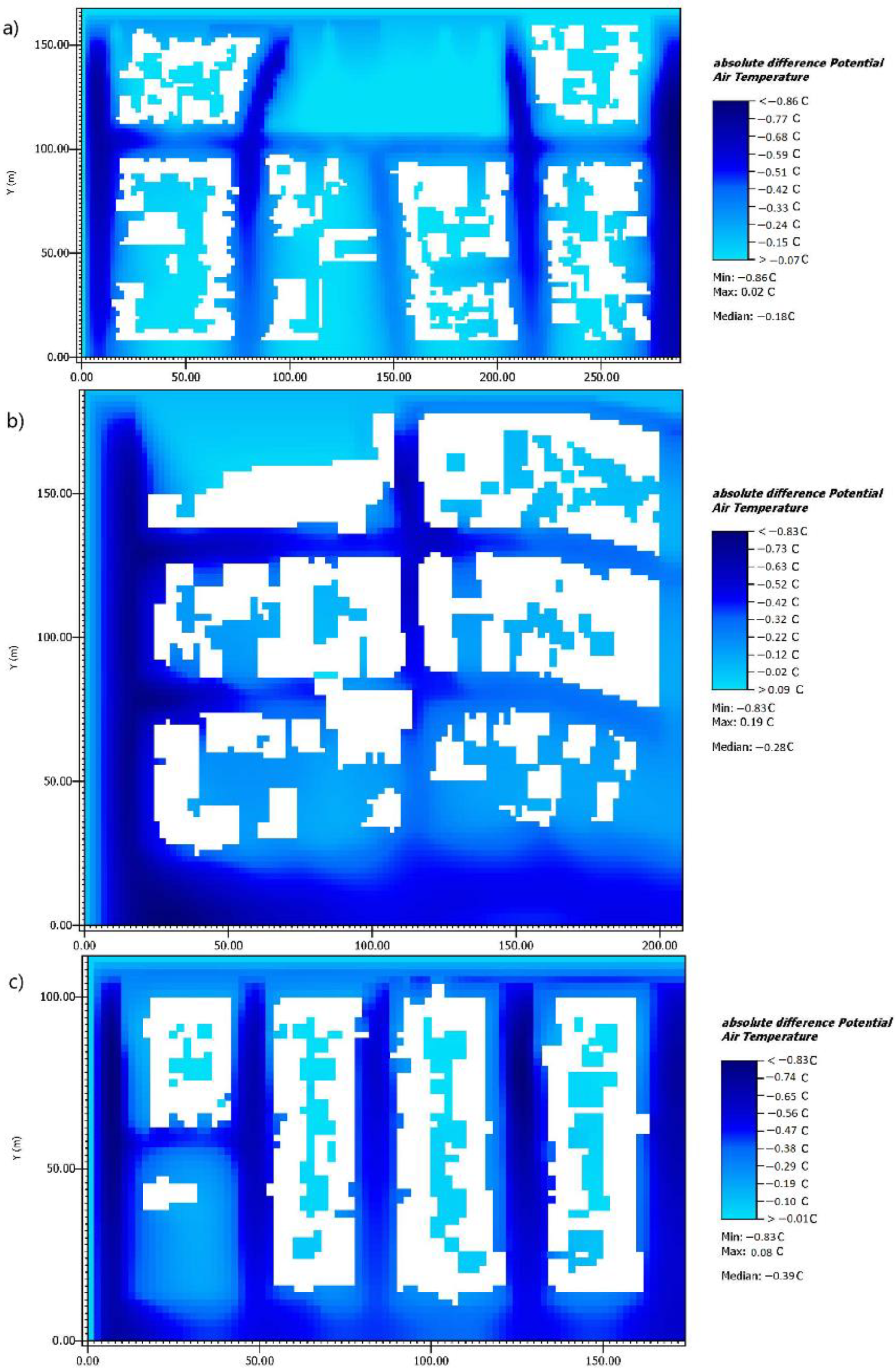
3.3. Air Temperature Difference
The analysis of the difference in air temperature between the baseline and mitigation scenarios, through the use of heat maps, allowed us to appreciate the thermal variations of the air in the study zones. These results can be seen in Figure 7. The air temperature in Zone A (Figure 7a) demonstrated a decrease of between 0.5 and 0.86 °C over its roadway. A decrease of between 0.07 and 0.5 °C could be seen in places where buildings were implemented. Zone A registered an average air temperature difference of 0.18 °C between the two scenarios. The air temperature difference in Zone B, represented in Figure 7b, showed the most critical thermal variations, with an observed decrease of between 0.42 and 0.83 °C, and the global average temperature of Zone B showed a decrease of 0.28 °C. Lastly, the analysis of the air temperature difference between the base and mitigation models for Zone C (Figure 7c) showed a thermal decrease over its roadway of between 0.47 and 0.83 °C, and the global average air temperature of the zone showed a 0.39 °C decrease.
In short, the difference in air temperature between the simulated and base scenarios allowed us to observe that the replacement of asphalt with cold pavements directly influenced the decrease in the global average temperature of the analysis zones.
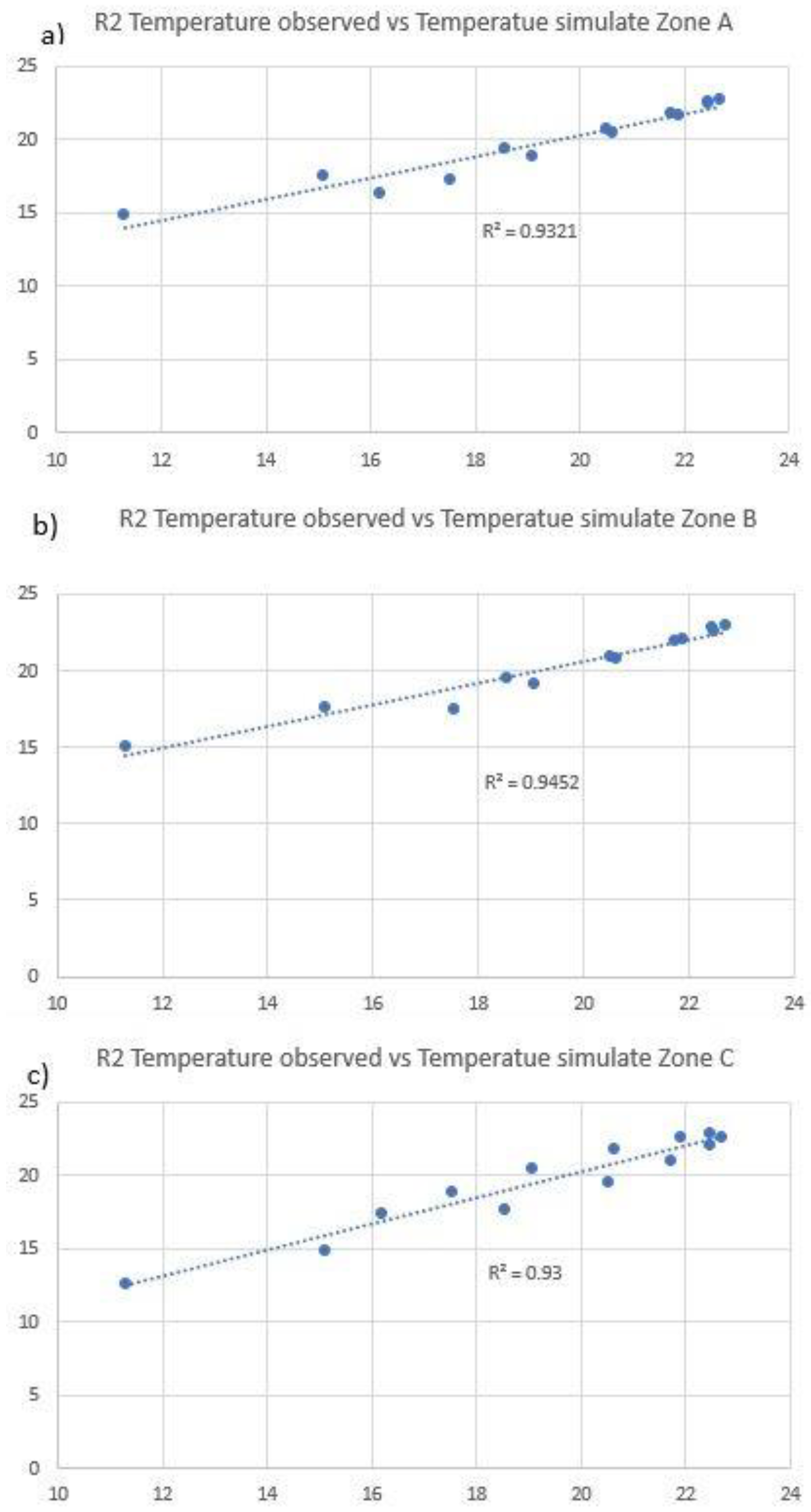
4. Validation
Figure 8 shows the results of the comparison between the observed and simulated air temperatures for the three study zones using the analysis of the coefficient of determination as the validation method of the simulated models. In this study, the R2 concerning air temperature in Zone A was equal to 0.93 (Figure 8a). Furthermore, Zone B registered an R2 value of 0.95 (Figure 8b), and Zone C registered an R2 value of 0.93 (Figure 8c). This means that the observed and simulated values of air temperatures of all zones were strongly correlated.
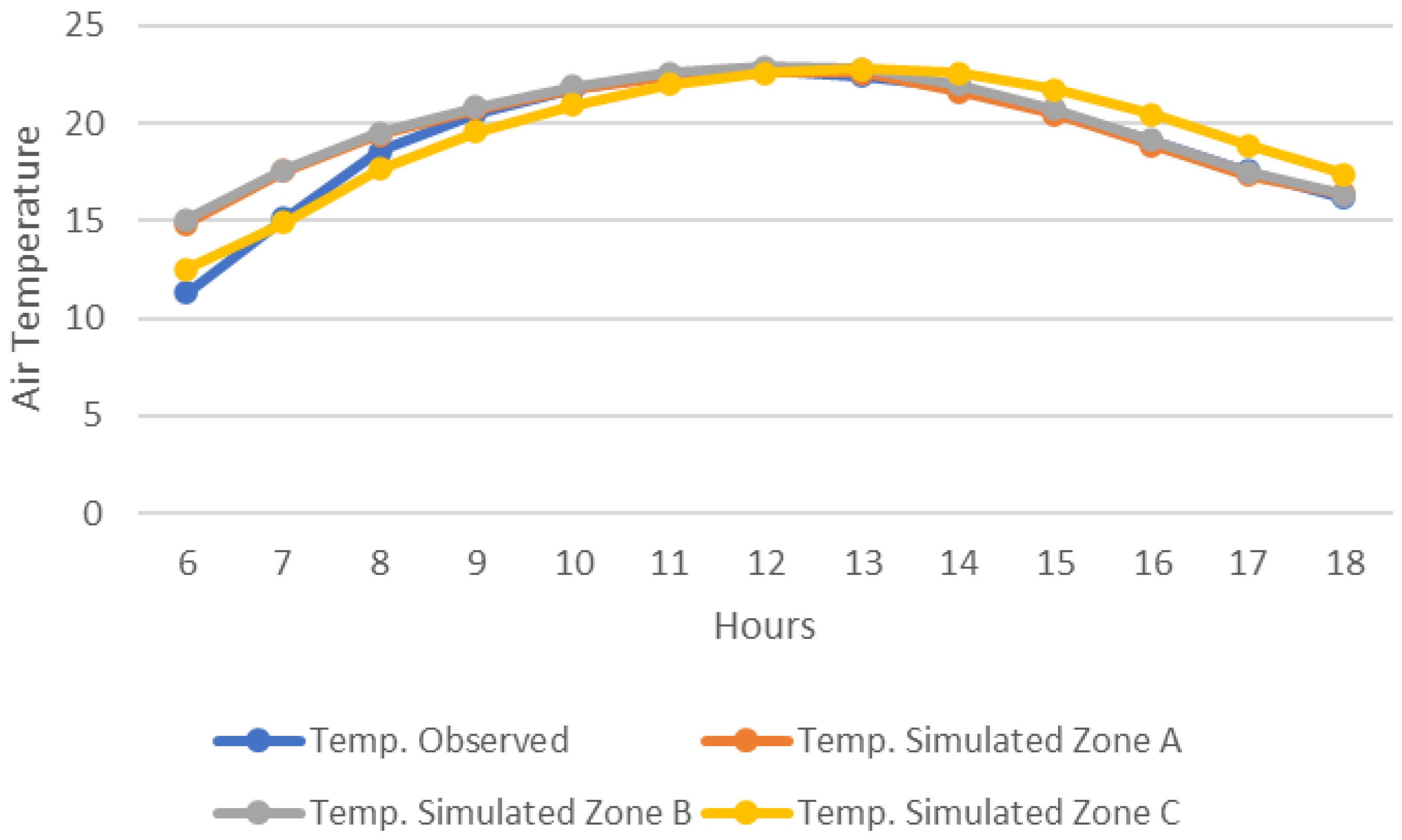
In Figure 9, the air temperature variations of the results of the three base scenarios and the observed air temperature over the same zones are shown graphically for the 12 continuous hours of the analysis. Thus, it is evident that the simulated air temperature values similarly fluctuated to the observed air temperature.
5. Discussion
As shown in the analysis carried out in three zones of Cuenca, replacing asphalt with concrete on roads proved to be beneficial for reducing LST (8 °C) and air temperature (0.86 °C). In addition, the findings of this study suggest that the high reflectivity of these pavements does not increase the temperature of building surfaces, possibly as a consequence of the reflection effect because the height of most buildings in the analyzed zones does not exceed 9 m. As suggested by Noelia et al. [61], this mitigation measure is effective. On the other hand, Qin et al. [62] concluded that to achieve optimal results for mitigating UHI effects, the areas where road materials are replaced with those that have higher albedo indexes must have a proportionality less than or equal to 1.5 between the height of buildings and the width of roads; when these measures are considered, solar radiation reflected by roads is not absorbed by the surfaces of buildings, thus avoiding the thermal discomfort of its inhabitants. Another strategy to improve asphalt reflectance is to add titanium dioxide-based dyes to the asphalt mixture, which can achieve similar results to those of concrete pavements according to Zheng et al. [63]. In addition, there are other mitigation alternatives such as those proposed by Cortes et al. [64]; in their UHI simulation analysis, carried out in Mandaue City on Cebu Island, adding green roofs and vegetation helped decrease air temperature and LST by 0.4 and 1.1 °C, respectively. For this type of mitigation strategy, vegetation height plays an important role in cooling surfaces [65].
For all analyzed zones, it was also observed that the average thermal difference of the roads (between base and mitigation scenarios) was approximately 8 °C. This result is comparable with those obtained by Ambrosini et al. [66], who carried out their study in the small town of Teramo (Italy). Teramo shares similar climatic characteristics with Cuenca, as its temperatures range between 11 and 22 °C. In their study, a similar thermal decrease was observed during the hottest hours of the day. Their analysis was based on mitigation simulations using cool pavements, but unlike this study, it also included green roofs. On the other hand, in a study conducted by Faragallah et al. [57] in Alexandria (Egypt), a city that has a warm desert climate, the following factors were added to the mitigation scenario: vegetation, trees, and small bodies of water. In addition, basalt was used for roads and concrete was used for sidewalks. Under these conditions, a reduction of 3 °C in global LST was archived. The findings are significantly similar to the ones obtained in this study, i.e., a 2.83 °C average decrease in global LST. Moreover, in all the previously analyzed zones, the surface temperature of the asphalt layer reached 40 °C, which was higher than the ambient temperature (20 °C).
Urban expansion and the rapid densification of cities accentuate the effect of UHIs, as demonstrated by Rahman et al. [17]. In their study, a remote sensing and geospatial tool analysis was carried out in the major districts of Bangladesh, where it was evident that land-use changes by urbanization increased LST in the winter seasons from 3 to 8 °C and a cool pavement-based mitigation proposal (such as the one used in this analysis that decreased the LST by 8 °C) could be used to mitigate the effects of UHI due to urbanization.
The findings of this study concerning air temperature indicated decreases of up to 0.83 °C over roads, and it was observed that average air temperature of the studied zones decreased by approximately 0.45 °C in the mitigation scenarios. These findings can be compared with those of Crank et al. [42], who used a similar mitigation design, in which a temperature decrease of up to 0.20 °C was observed. Additionally, Zhang et al. [60] obtained a decrease in mean air temperature of up to 1.5 °C by including green roofs in their mitigation scenarios. Furthermore, the study conducted by Faragallah et al. [57] in the city of Alexandria Egypt demonstrated that combinations of cool pavements with vegetation and water bodies in urban environments could decrease air temperature by up to 3.5 °C.
6. Conclusions
It is possible to mitigate the urban heat island effect by using more reflective materials or materials with higher albedo indices for urban roads. The results of this research revealed that there was a decrease in surface temperature that led to a decrease in average air temperature in all analyzed areas when replacing asphalt with concrete pavements.
On average, in the mitigation scenarios, the road surface temperatures decreased by 8 °C. On the other hand, the overall LST decreased by 3 °C, and the average air temperature decreased by 0.45 °C on average; the air temperature over the roads also registered a decrease of up to 0.86 °C. The areas with vegetation cover in the three studied zones showed an LST decrease of between 1 and 2 °C, and the air temperature in these areas registered an average decrease of 0.25 °C. At the same time, surface temperatures did not change in the building areas, which could indicate no changes in their thermal comfort as measured with an equivalent physiological temperature index.
Wind direction and speed play important roles in the cooling of surfaces. In this study, Zone A registered a significant decrease of approximately 4 °C in the LST of the road surface due to the roads being located in the direction of the wind flow, and the air temperature above the roads was reduced by up to 0.83 °C. In turn, in areas where wind circulation is limited, thermal variations were not significant, especially in the spaces of buildings and narrow alleys where temperatures decreased, though not with the same intensity as in open spaces or areas with favorable circulation for air exchange.
This analysis was carried out with the ENVI-met software, student version 5.0.0. In this version, the processing capacity of the computer is limited to a single core. The limited processing capacity prevented the analysis of the study areas at higher resolutions due to their size. Higher resolution heat maps would require a lot of time and computational resources. For more accurate results, it is recommended to use additional climatic parameters, such as relative humidity, precipitation, temperature, cloudiness, solar radiation, and wind speed. In addition, for future complementary research, it is recommended to incorporate other sustainable alternatives, such as green roofs and increased vegetation cover, in the mitigation scenarios of the analyzed areas to more accurately assess the behavior of UHIs.
The results of this study can be used by government agencies or urban planners to make better decisions regarding the creation of more sustainable cities and more comfortable spaces for their inhabitants.
Author Contributions
Conceptualization, P.E.V.-Á. and S.L.C.-M.; methodology, S.L.C.-M. and J.-C.C.-T.; software, P.E.V.-Á.; validation, P.E.V.-Á.; formal analysis, P.E.V.-Á.; investigation, P.E.V.-Á.; resources, S.L.C.-M.; data curation, P.E.V.-Á.; writing—original draft preparation, P.E.V.-Á.; writing—review and editing, P.E.V.-Á. and S.L.C.-M.; visualization, P.E.V.-Á.; supervision, S.L.C.-M. and C.F.-V.; project administration, S.L.C.-M.; funding acquisition, S.L.C.-M. and J.-C.C.-T. All authors have read and agreed to the published version of the manuscript.
Funding
This project was funded by Catholic University of Cuenca by funding number UCACUE-JIEI-2021-241-OF.
Institutional Review Board Statement
Not applicable.
Informed Consent Statement
Not applicable.
Data Availability Statement
Not applicable.
Acknowledgments
This manuscript is part of a Master’s Program in Construction with a Major in the Sustainable Construction Management Catholic University of Cuenca. It is also linked to the “Urban Sustainability Indicators for the City of Cuenca—Ecuador” Research Project. In addition, we would like to thank all professors part of the following research groups: City, Environment, and Technology; Embedded Systems and Artificial Vision in Architectural, Agricultural, Environmental and Automatic Sciences (SEVA4CA); and Urban and Earth Data Science for knowledge and information provided for carrying out this study.
Conflicts of Interest
The authors declare no conflict of interest.
References
- Zhou, D.; Xiao, J.; Bonafoni, S.; Berger, C.; Deilami, K.; Zhou, Y.; Frolking, S.; Yao, R.; Qiao, Z.; Sobrino, J.A. Satellite remote sensing of surface urban heat islands: Progress, challenges, and perspectives. Remote Sens. 2019, 11, 48. [Google Scholar] [CrossRef] [Green Version]
- Singh, P.; Kikon, N.; Verma, P. Impact of land use change and urbanization on urban heat island in Lucknow city, Central India. A remote sensing based estimate. Sustain. Cities Soc. 2017, 32, 100–114. [Google Scholar] [CrossRef]
- Zhang, X.; Estoque, R.C.; Murayama, Y. An urban heat island study in Nanchang City, China based on land surface temperature and social-ecological variables. Sustain. Cities Soc. 2017, 32, 557–568. [Google Scholar] [CrossRef]
- Manoli, G.; Fatichi, S.; Schläpfer, M.; Yu, K.; Crowther, T.W.; Meili, N.; Burlando, P.; Katul, G.G.; Bou-Zeid, E. Magnitude of urban heat islands largely explained by climate and population. Nature 2019, 573, 55–60. [Google Scholar] [CrossRef] [PubMed]
- Tumini, I. El microclima Urbano en los Espacios Abiertos: Estudio de Casos en Madrid; Universidad Politécnica de Madrid: Madrid, Spain, 2012. [Google Scholar]
- Herath, H.M.P.I.K.; Halwatura, R.U.; Jayasinghe, G.Y. Modeling a Tropical Urban Context with Green Walls and Green Roofs as an Urban Heat Island Adaptation Strategy. Procedia Eng. 2018, 212, 691–698. [Google Scholar] [CrossRef]
- Chen, T.; Sun, A.; Niu, R. Effect of Land Cover Fractions on Changes in Surface Urban Heat Islands Using Landsat Time-Series Images. Int. J. Environ. Res. Public Health 2019, 16, 971. [Google Scholar] [CrossRef] [Green Version]
- Torok, S.J.; Morris, C.J.G.; Skinner, C.; Plummer, N. Urban heat island features of southeast Australian towns. Aust. Meteorol. Mag. 2001, 50, 1–13. [Google Scholar]
- Ghobadi, A.; Khosravi, M.; Tavousi, T. Surveying of Heat waves Impact on the Urban Heat Islands: Case study, the Karaj City in Iran. Urban Clim. 2018, 24, 600–615. [Google Scholar] [CrossRef]
- Sharifi, E.; Lehmann, S. Comparative analysis of surface urban heat island effect in central sydney. J. Sustain. Dev. 2014, 7, 23–34. [Google Scholar] [CrossRef] [Green Version]
- Campoverde, A.S.B. Analysis of the urban heat island in the Andean environment of Cuenca-Ecuador. Investig. Geogr. 2018, 167–179. [Google Scholar] [CrossRef] [Green Version]
- Li, X.; Zhou, Y.; Asrar, G.R.; Imhoff, M.; Li, X. The surface urban heat island response to urban expansion: A panel analysis for the conterminous United States. Sci. Total Environ. 2017, 605–606, 426–435. [Google Scholar] [CrossRef] [PubMed]
- Debbage, N.; Shepherd, J.M. The urban heat island effect and city contiguity. Comput. Environ. Urban Syst. 2015, 54, 181–194. [Google Scholar] [CrossRef]
- Niu, L.; Tang, R.; Jiang, Y.; Zhou, X. Spatiotemporal patterns and drivers of the surface urban heat island in 36 major cities in China: A comparison of two different methods for delineating rural areas. Sustainbility 2020, 12, 478. [Google Scholar] [CrossRef] [Green Version]
- Mohajerani, A.; Bakaric, J.; Jeffrey-Bailey, T. The urban heat island effect, its causes, and mitigation, with reference to the thermal properties of asphalt concrete. J. Environ. Manag. 2017, 197, 522–538. [Google Scholar] [CrossRef] [PubMed]
- Ferrelli, F.; Bustos, M.Y.; Piccolo, M. Modificaciones en la distribución espacial de la temperatura y la humedad relativa como resultado del crecimiento urbano: El caso de la ciudad de Bahía Blanca, Argentina. Rev. Climatol. 2016, 16, 51–61. [Google Scholar]
- Rahman, M.N.; Rony, M.R.H.; Jannat, F.A.; Pal, S.C.; Islam, M.S.; Alam, E.; Islam, A.R.M.T. Impact of Urbanization on Urban Heat Island Intensity in Major Districts of Bangladesh Using Remote Sensing and Geo-Spatial Tools. Climate 2022, 10, 3. [Google Scholar] [CrossRef]
- Ranagalage, M.; Estoque, R.C.; Zhang, X.; Murayama, Y. Spatial changes of urban heat island formation in the Colombo District, Sri Lanka: Implications for sustainability planning. Sustainbility 2018, 10, 1367. [Google Scholar] [CrossRef] [Green Version]
- ONU-Habitad Hacer de la Densidad una Variable Fundamental Disponible en. Available online: https://onuhabitat.org.mx/index.php/hacer-de-la-densidad-una-variable-fundamental (accessed on 18 May 2021).
- Heaviside, C.; Macintyre, H.; Vardoulakis, S. The Urban Heat Island: Implications for Health in a Changing Environment. Curr. Environ. Health Rep. 2017, 4, 296–305. [Google Scholar] [CrossRef]
- Hassid, S.; Santamouris, M.; Papanikolaou, N.; Linardi, A.; Klitsikas, N.; Georgakis, C.; Assimakopoulos, D.N. Effect of the Athens heat island on air conditioning load. Energy Build 2000, 32, 131–141. [Google Scholar] [CrossRef]
- Sarrat, C.; Lemonsu, A.; Masson, V.; Guedalia, D. Impact of urban heat island on regional atmospheric pollution. Atmos. Environ. 2006, 40, 1743–1758. [Google Scholar] [CrossRef]
- Marando, F.; Heris, M.P.; Zulian, G.; Udías, A.; Mentaschi, L.; Chrysoulakis, N.; Parastatidis, D.; Maes, J. Urban heat island mitigation by green infrastructure in European Functional Urban Areas. Sustain. Cities Soc. 2022, 77, 103564. [Google Scholar] [CrossRef]
- Narváez, T.; Contreras, C. Metodología de Análisis Para Mitigar el Efecto de la Isla del Calor Urbano de la Ciudad de Cuenca Con énfasis en los Pavimentos de Hormigón; Universidad Católica de Cuenca: Cuenca, Ecuador, 2019. [Google Scholar]
- Ernesto, M.; Correa, D. Análisis crítico de la planificación urbana de la Ciudad de Cuenca. Maskana 2016, 7, 107–122. [Google Scholar]
- Cobo, L. Isla de Calor por la Incidencia de los Fenómenos de Tranferencia en Pavimentos Flexibles en la Ciudad de Riobamba; Universidad Nacional de Chimborazo: Riobamba, Ecuador, 2020. [Google Scholar]
- Sen, S.; Roesler, J. Thermal and optical characterization of asphalt field cores for microscale urban heat island analysis. Constr. Build. Mater. 2019, 217, 600–611. [Google Scholar] [CrossRef]
- Correa, E.N.; Flores Larsen, S.; Lesino, G. Isla de calor urbana: Efecto de los pavimentos. Av. Energías Renov. Medio Ambient. 2003, 7, 25–30. [Google Scholar]
- Ibrahim, S.H.; Ibrahim, N.I.A.; Wahid, J.; Goh, N.A.; Koesmeri, D.R.A.; Nawi, M.N.M. The impact of road pavement on urban heat island (UHI) phenomenon. Int. J. Technol. 2018, 9, 1597–1608. [Google Scholar] [CrossRef] [Green Version]
- Maleki, A.; Mahdavi, A. Evaluation of Urban Heat Islands Mitigation Strategies Using 3dimentional Urban Micro-Climate Model Envi-Met. ASIAN J. Civ. Eng. 2016, 17, 357–371. [Google Scholar]
- Pisello, A.L.; Pignatta, G.; Castaldo, V.L.; Cotana, F. Experimental analysis of natural gravel covering as cool roofing and cool pavement. Sustainbility 2014, 6, 4706–4722. [Google Scholar] [CrossRef] [Green Version]
- Zhang, L.; Fukuda, H.; Liu, Z. The value of cool roof as a strategy to mitigate urban heat island effect: A contingent valuation approach. J. Clean. Prod. 2019, 228, 770–777. [Google Scholar] [CrossRef]
- Santamouris, M. Using cool pavements as a mitigation strategy to fight urban heat island-A review of the actual developments. Renew. Sustain. Energy Rev. 2013, 26, 224–240. [Google Scholar] [CrossRef]
- Sen, S.; Roesler, J.; Ruddell, B.; Middel, A. Cool pavement strategies for Urban Heat Island mitigation in Suburban Phoenix, Arizona. Sustainbility 2019, 11, 4452. [Google Scholar] [CrossRef] [Green Version]
- Kyriakodis, G.E.; Santamouris, M. Using reflective pavements to mitigate urban heat island in warm climates-Results from a large scale urban mitigation project. Urban Clim. 2018, 24, 326–339. [Google Scholar] [CrossRef]
- Machado, J. La temperatura en Quito no deja de subir desde 2004. Available online: primicias.ec/noticias/sociedad/temperatura-quito-calor-calentamiento-global/ (accessed on 18 September 2021).
- Guillén Mena, V.; Orellana Valdez, D. Un acercamiento a caracterizar la isla de calor en Cuenca, Ecuador. In Proceedings of the Congreso Nacional del Medio Ambiente Conama 2016, Madrid, España, 1–28 December 2016; pp. 1–16. [Google Scholar]
- Bustamante Campoverde, A.; Orellana Valdez, D. Caracterización de la isla de calor urbana en Cuenca (Ecuador). Efectos de la morfología urbana. In Proceedings of the Congreso Internacional I+D+i en sosteniblidad energética INER 2017, Quito, Ecuador, 20–22 September 2017; pp. 10–18. [Google Scholar]
- He, B.J.; Wang, J.; Liu, H.; Ulpiani, G. Localized synergies between heat waves and urban heat islands: Implications on human thermal comfort and urban heat management. Environ. Res. 2021, 193, 110584. [Google Scholar] [CrossRef] [PubMed]
- Kubilay, A.; Allegrini, J.; Strebel, D.; Zhao, Y.; Derome, D.; Carmeliet, J. Advancement in urban climate modelling at local scale: Urban heat island mitigation and building cooling demand. Atmosphere 2020, 11, 1313. [Google Scholar] [CrossRef]
- Fernández, Q.V. Simulación con Modelos Climáticos en Infraestructuras de Computación Distribuida; Universidad de Cantabria: Cantabria, Spain, 2020. [Google Scholar]
- Crank, P.J.; Sailor, D.J.; Ban-Weiss, G.; Taleghani, M. Evaluating the ENVI-met microscale model for suitability in analysis of targeted urban heat mitigation strategies. Urban Clim. 2018, 26, 188–197. [Google Scholar] [CrossRef]
- Yilmaz, S.; Mutlu, E.; Yilmaz, H. Alternative scenarios for ecological urbanizations using ENVI-met model. Environ. Sci. Pollut. Res. 2018, 25, 26307–26321. [Google Scholar] [CrossRef]
- Mutlu, B.E.; Yilmaz, S. Evaluation of the Effect of Green Areas on Thermal Comfort in Urban Areas with Microscale ENVI-Met Software. In Proceedings of the PACE 2021, Erzurum, Turkey, 20–23 June 2021; pp. 1–5. [Google Scholar]
- Instituto Nacional de Estadísticas y Censos. Fascículo Provincial Azuay. Equipo Comun. y Análisis del Censo Población y Vivienda. INEC 2010, 1, 8. [Google Scholar]
- Quezada, M.F. Lineamientos Metodológicos Para Ordenar el Área Periurbana de Cuenca: Caso Guncay-El Valle; Universidad de Cuenca: Cuenca, Ecuador, 2015. [Google Scholar]
- Pinos-Arévalo, N. Prospective land use and vegetation cover on land management-Case canton Cuenca. Estoa 2016, 5, 7–19. [Google Scholar] [CrossRef] [Green Version]
- Kottek, M.; Grieser, J.; Beck, C.; Rudolf, B.; Rubel, F. World map of the Köppen-Geiger climate classification updated. Meteorol. Z. 2006, 15, 259–263. [Google Scholar] [CrossRef]
- Barragán, A.E.; Ochoa, P.E. Diseño de viviendas ambientales de bajo costo. Maskana 2014, 5, 81–98. [Google Scholar] [CrossRef] [Green Version]
- Ozkeresteci, I.; Crewe, K.; Brazel, A.J.; Bruse, M. Use and evaluation of the ENVI-met model for environmental design and planning. An Experiment on Lienar Parks. In Proceedings of the 21st International Cartographic Conference (ICC), Durban, South Africa, 10–16 August 2003; pp. 10–16. [Google Scholar]
- Elnabawi, M.H.; Hamza, N.; Dudek, S. Use and evaluation of the envi-met model for two different urban forms in cairo, egypt: Measurements and model simulations. In Proceedings of the 3th Conference of International Building Performance Simulation Association, Chambéry, France, 25–28 August 2013; pp. 2800–2806. [Google Scholar]
- Sun, S.; Xu, X.; Lao, Z.; Liu, W.; Li, Z.; Higueras García, E.; He, L.; Zhu, J. Evaluating the impact of urban green space and landscape design parameters on thermal comfort in hot summer by numerical simulation. Build. Environ. 2017, 123, 277–288. [Google Scholar] [CrossRef]
- NASA Power Ceres Merra 2 Daily Data. Available online: Power.larc.nasa.gov/data-access-viewer (accessed on 9 September 2021).
- Bosilovich, M.G.; Lucchesi, R.; Suarez, M. MERRA-2: File Specification. Earth 2016, 9, 73. [Google Scholar]
- Gelaro, R.; McCarty, W.; Suárez, M.J.; Todling, R.; Molod, A.; Takacs, L.; Randles, C.A.; Darmenov, A.; Bosilovich, M.G.; Reichle, R.; et al. The modern-era retrospective analysis for research and applications, version 2 (MERRA-2). J. Clim. 2017, 30, 5419–5454. [Google Scholar] [CrossRef] [PubMed]
- ENVI-met GmbH Emvi-met V5 2021. Available online: Envi-met.com/landscape-architects/ (accessed on 14 October 2021).
- Faragallah, R.N.; Ragheb, R.A. Evaluation of thermal comfort and urban heat island through cool paving materials using ENVI-Met. Ain Shams Eng. J. 2022, 13, 101609. [Google Scholar] [CrossRef]
- Elwy, I.; Ibrahim, Y.; Fahmy, M.; Mahdy, M. Outdoor microclimatic validation for hybrid simulation workflow in hot arid climates against ENVI-met and field measurements. Energy Procedia 2018, 153, 29–34. [Google Scholar] [CrossRef]
- Abaas, Z.R. Impact of development on Baghdad’s urban microclimate and human thermal comfort. Alexandria Eng. J. 2020, 59, 275–290. [Google Scholar] [CrossRef]
- Zhang, L.; Zhan, Q.; Lan, Y. Effects of the tree distribution and species on outdoor environment conditions in a hot summer and cold winter zone: A case study in Wuhan residential quarters. Build. Environ. 2018, 130, 27–39. [Google Scholar] [CrossRef]
- Alchapar, N.L.; Correa, E.N. The use of reflective materials as a strategy for urban cooling in an arid “OASIS” city. Sustain. Cities Soc. 2016, 27, 1–14. [Google Scholar] [CrossRef]
- Qin, Y. Urban canyon albedo and its implication on the use of reflective cool pavements. Energy Build. 2015, 96, 86–94. [Google Scholar] [CrossRef]
- Zheng, N.; Lei, J.; Wang, S.; Li, Z.; Chen, X. Influence of heat reflective coating on the cooling and pavement performance of large void asphalt pavement. Coatings 2020, 10, 1065. [Google Scholar] [CrossRef]
- Cortes, A.; Rejuso, A.J.; Santos, J.A.; Blanco, A. Evaluating mitigation strategies for urban heat island in Mandaue City using ENVI-met. J. Urban Manag. 2022, 11, 97–106. [Google Scholar] [CrossRef]
- Baloloy, A.; Cruz, J.A.; Sta Ana, R.R.; Blanco, A.; Lubrica, N.V.; Valdez, C.J.; Bernardo, J.J. Modelling and simulation of potential future urbanization scenarios and its effect on the microclimate of lower session road, baguio city. ISPRS Ann. Photogramm. Remote Sens. Spat. Inf. Sci. 2020, 5, 187–194. [Google Scholar] [CrossRef]
- Ambrosini, D.; Galli, G.; Mancini, B.; Nardi, I.; Sfarra, S. Evaluating mitigation effects of urban heat islands in a historical small center with the ENVI-Met® climate model. Sustainability 2014, 6, 7013–7029. [Google Scholar] [CrossRef] [Green Version]
Figure 1.
General location map of the study area in Ecuador.

Figure 2.
Workflow of computer simulations using ENVI-met.

Figure 3.
Zone locations (A, B, and C) for computer modeling.

Figure 4.
Scenarios digitized in the space module of ENVI-met software. Base scenarios (asphalt) are represented in (a–c), and mitigation scenarios (concrete) are represented in (d–f).
Figure 4.
Scenarios digitized in the space module of ENVI-met software. Base scenarios (asphalt) are represented in (a–c), and mitigation scenarios (concrete) are represented in (d–f).

Figure 5.
Surface temperature maps of studied zones. (a) Zone A—base scenario; (b) Zone A—mitigation scenario; (c) Zone B—base scenario; (d) Zone B—mitigation scenario; (e) Zone C—base scenario; (f) Zone C—mitigation scenario.
Figure 5.
Surface temperature maps of studied zones. (a) Zone A—base scenario; (b) Zone A—mitigation scenario; (c) Zone B—base scenario; (d) Zone B—mitigation scenario; (e) Zone C—base scenario; (f) Zone C—mitigation scenario.

Figure 6.
Surface temperature difference between base and mitigation scenarios: (a) Zone A, (b) Zone B, and (c) Zone C.
Figure 6.
Surface temperature difference between base and mitigation scenarios: (a) Zone A, (b) Zone B, and (c) Zone C.

Figure 7.
Air temperature difference between base and mitigation scenarios: (a) Zone A, (b) Zone B, and (c) Zone C.
Figure 7.
Air temperature difference between base and mitigation scenarios: (a) Zone A, (b) Zone B, and (c) Zone C.

Figure 8.
Comparison between simulated and measured air temperature on 22 January 2020 using R2. (a) Zone A, (b) Zone B, and (c) Zone C.
Figure 8.
Comparison between simulated and measured air temperature on 22 January 2020 using R2. (a) Zone A, (b) Zone B, and (c) Zone C.

Figure 9.
Hourly time series of observed vs. simulated average air temperatures on 22 January 2020.


Table 1.
Input weather parameters applied in the simulated scenarios.
| Meteorological Parameters | Unit |
|---|---|
| Minimum initial air temperature | 11 °C |
| Maximum air temperature | 20 °C |
| Wind speed | 2.5 m/s |
| Wind direction | 315° Northeast |
Table 2.
Thermophysical properties of materials applied in the simulated scenarios.
| Material | Albedo | Emissivity | Component |
|---|---|---|---|
| Asphalt | 0.2 | 0.9 | Roads |
| Used concrete | 0.3 | 0.9 | Roads/other |
| Concrete | 0.5 | 0.9 | Roads |
| Concrete | NA | NA | Walls |
| Tile | NA | NA | Roofs |
| Grass height of less than 25 cm | 0.2 | NA | Vegetation cover |
| Medium-sized, leafy trees | 0.2 | NA | Vegetation cover |
Publisher’s Note: MDPI stays neutral with regard to jurisdictional claims in published maps and institutional affiliations. |
© 2022 by the authors. Licensee MDPI, Basel, Switzerland. This article is an open access article distributed under the terms and conditions of the Creative Commons Attribution (CC BY) license (https://creativecommons.org/licenses/by/4.0/).
Share and Cite
MDPI and ACS Style
Vásquez-Álvarez, P.E.; Flores-Vázquez, C.; Cobos-Torres, J.-C.; Cobos-Mora, S.L. Urban Heat Island Mitigation through Planned Simulation. Sustainability 2022, 14, 8612. https://doi.org/10.3390/su14148612
AMA Style
Vásquez-Álvarez PE, Flores-Vázquez C, Cobos-Torres J-C, Cobos-Mora SL. Urban Heat Island Mitigation through Planned Simulation. Sustainability. 2022; 14(14):8612. https://doi.org/10.3390/su14148612
Chicago/Turabian StyleVásquez-Álvarez, Paul Eduardo, Carlos Flores-Vázquez, Juan-Carlos Cobos-Torres, and Sandra Lucía Cobos-Mora. 2022. "Urban Heat Island Mitigation through Planned Simulation" Sustainability 14, no. 14: 8612. https://doi.org/10.3390/su14148612
Note that from the first issue of 2016, this journal uses article numbers instead of page numbers. See further details here.