
Impact of Urbanization on Seismic Risk: A Study Based on Remote Sensing Data


Abstract
:1. Introduction
2. Materials and Methods
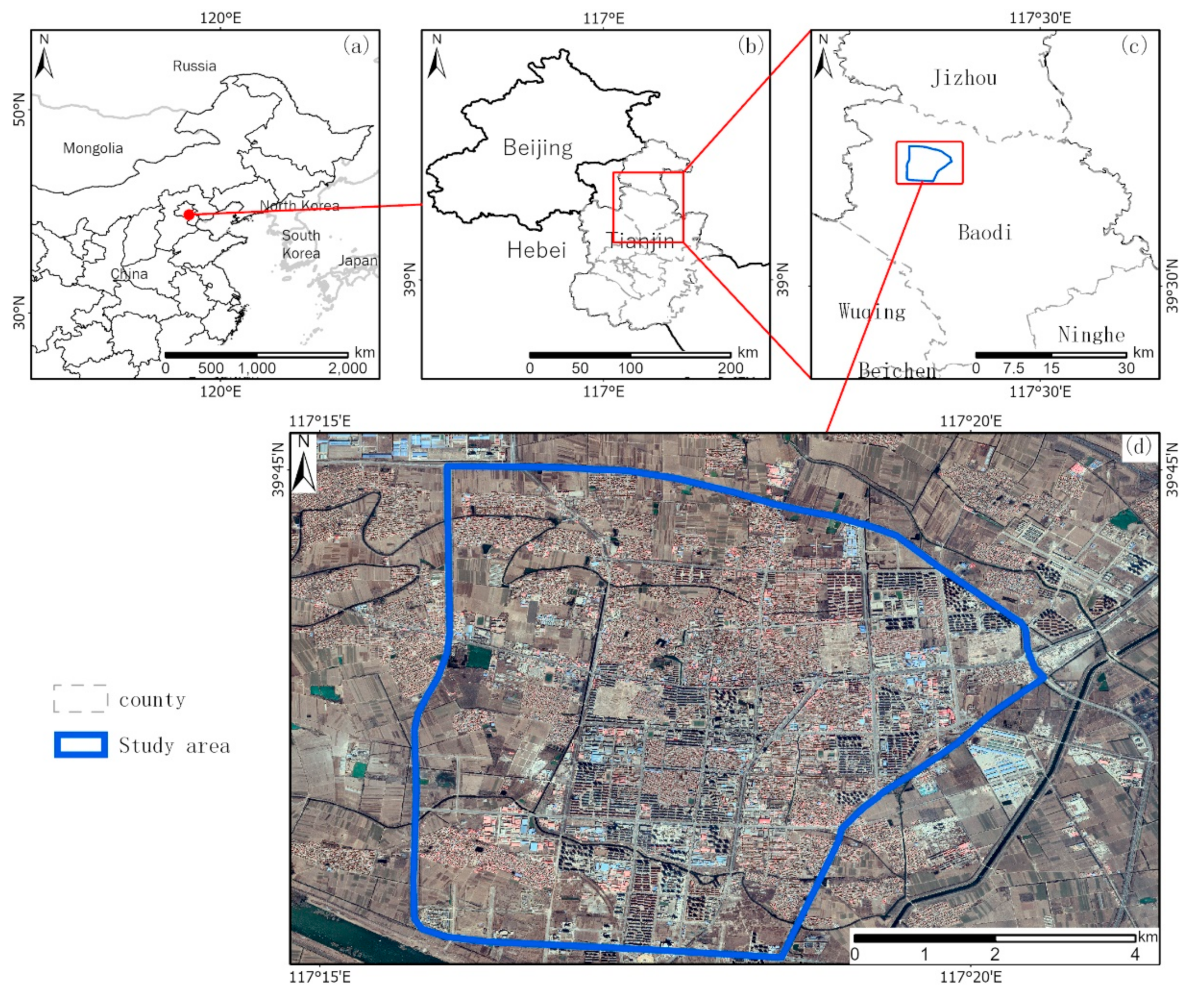
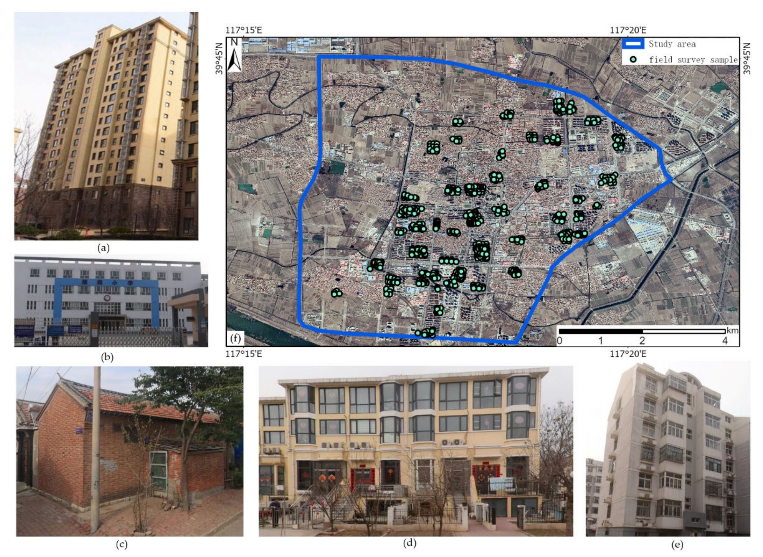
2.1. Study Area
2.2. Data Sources
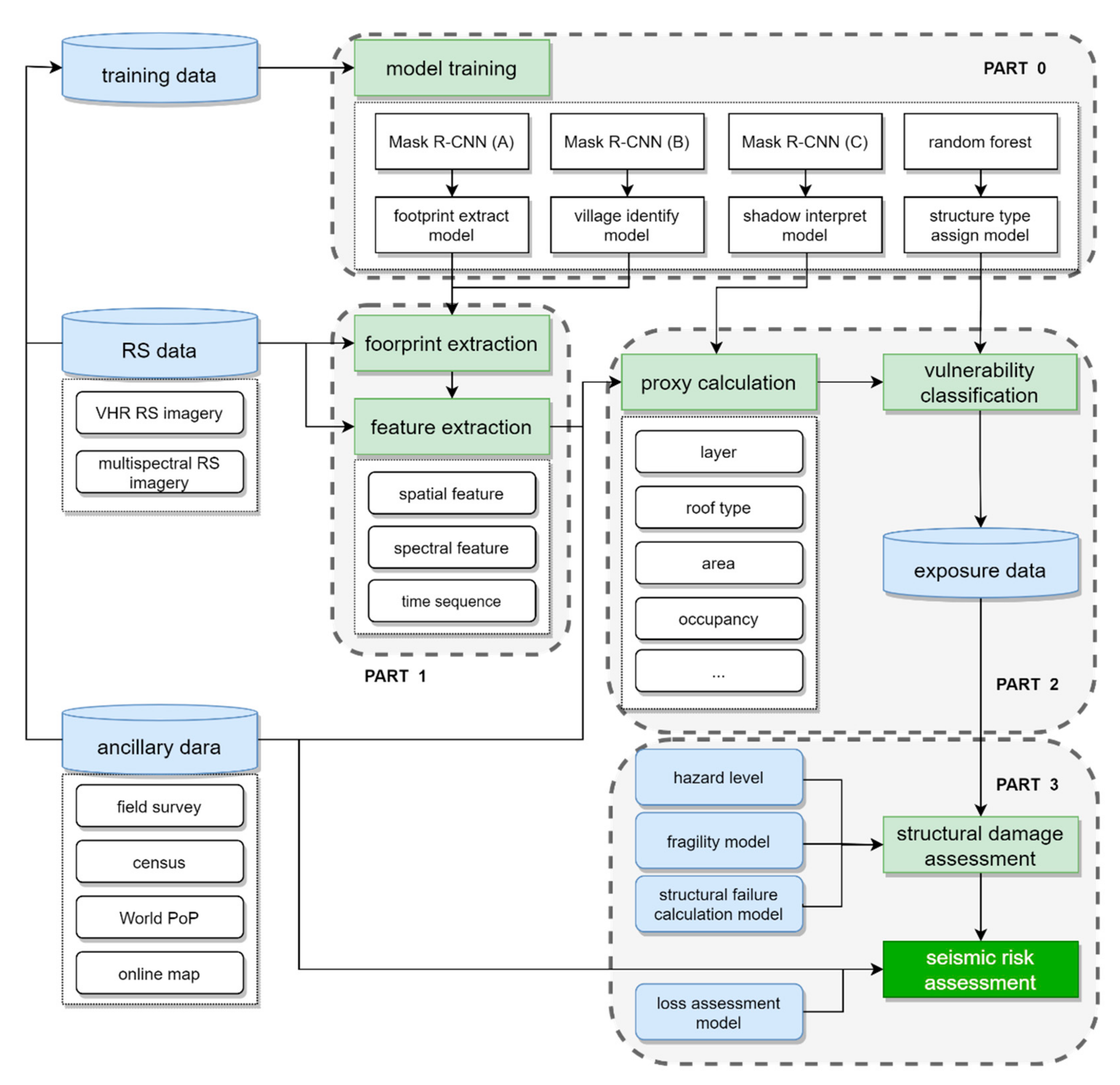
2.3. Overall Workflow
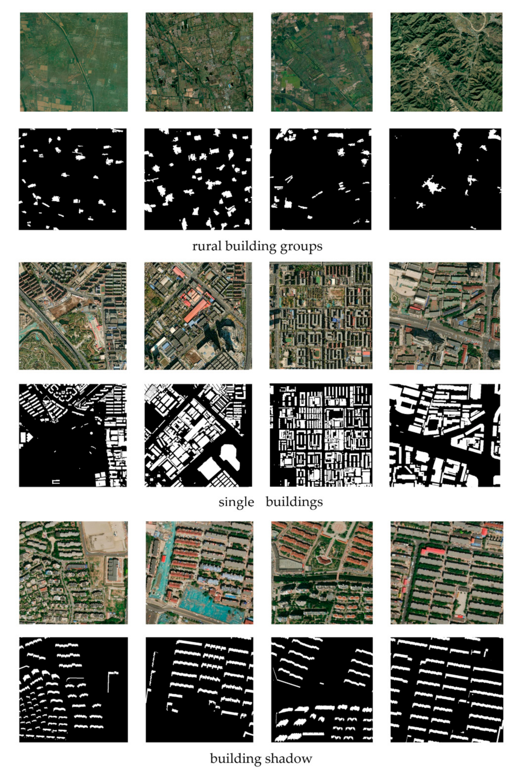
2.4. Building Feature Extraction
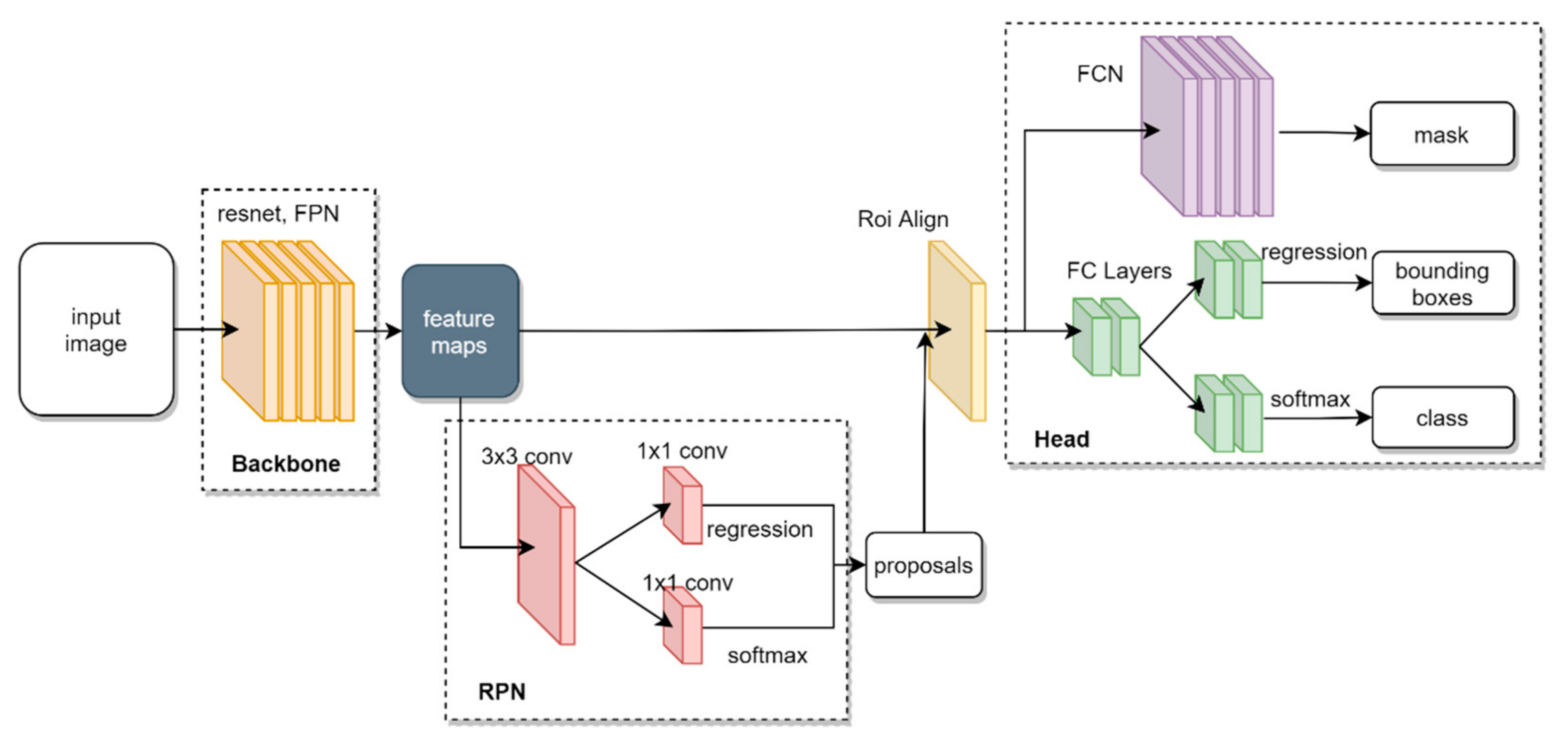
2.4.1. Mask R-CNN Framework
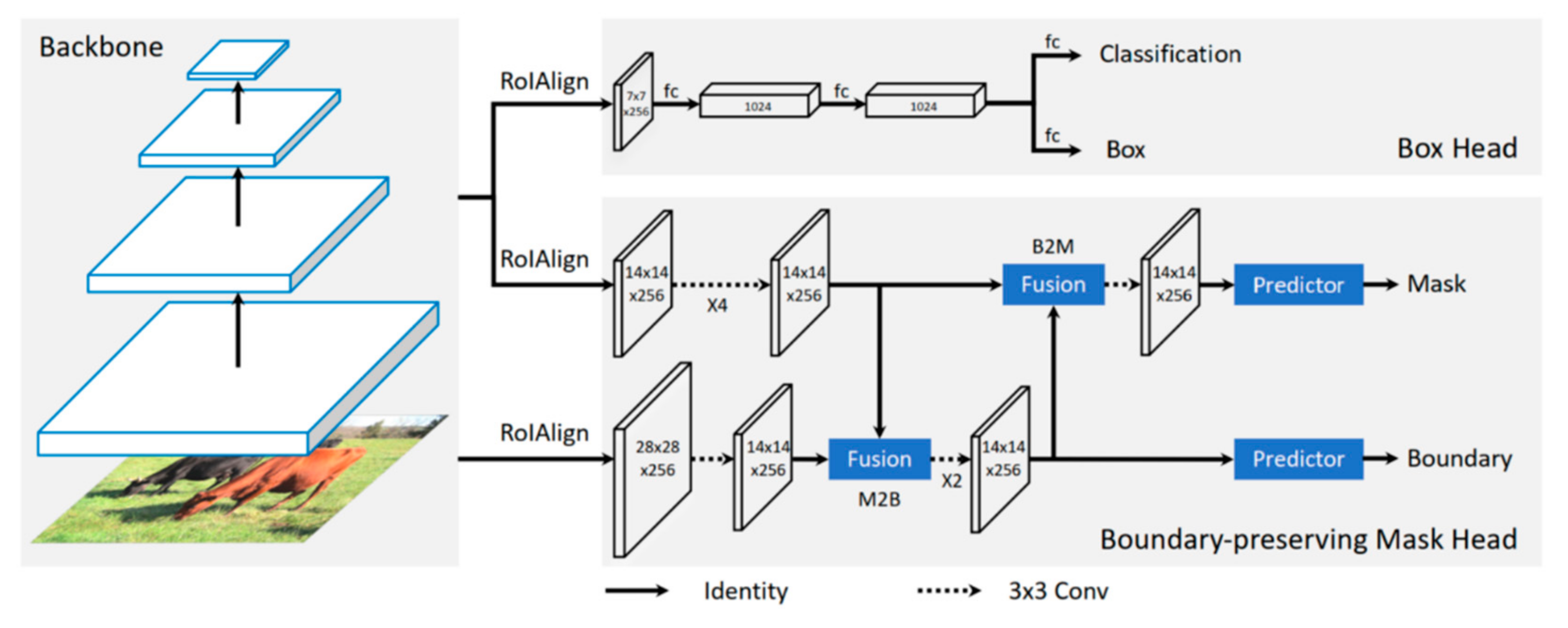
2.4.2. BMask R-CNN Framework
2.4.3. Post-Processing of Building Footprint
- (i)
- Eliminating non-structural misclassification by setting an area threshold;
- (ii)
- Intersecting single buildings and building groups, keeping single buildings in the rural building group, and eliminating redundancy in the two output footprints;
- (iii)
- Calculating the actual building area of the rural building group.
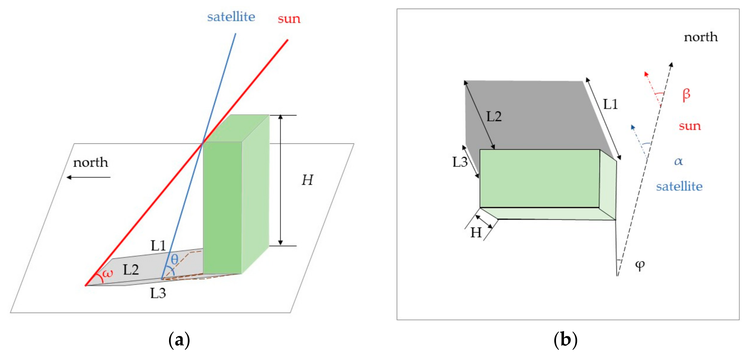
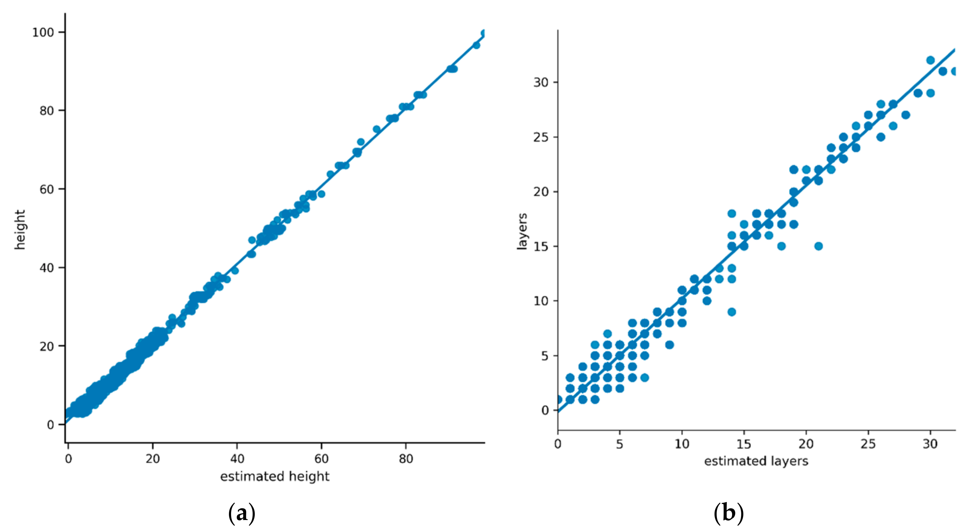
2.4.4. Estimating Floor Numbers
2.4.5. Occupancy and Population Disaggregation
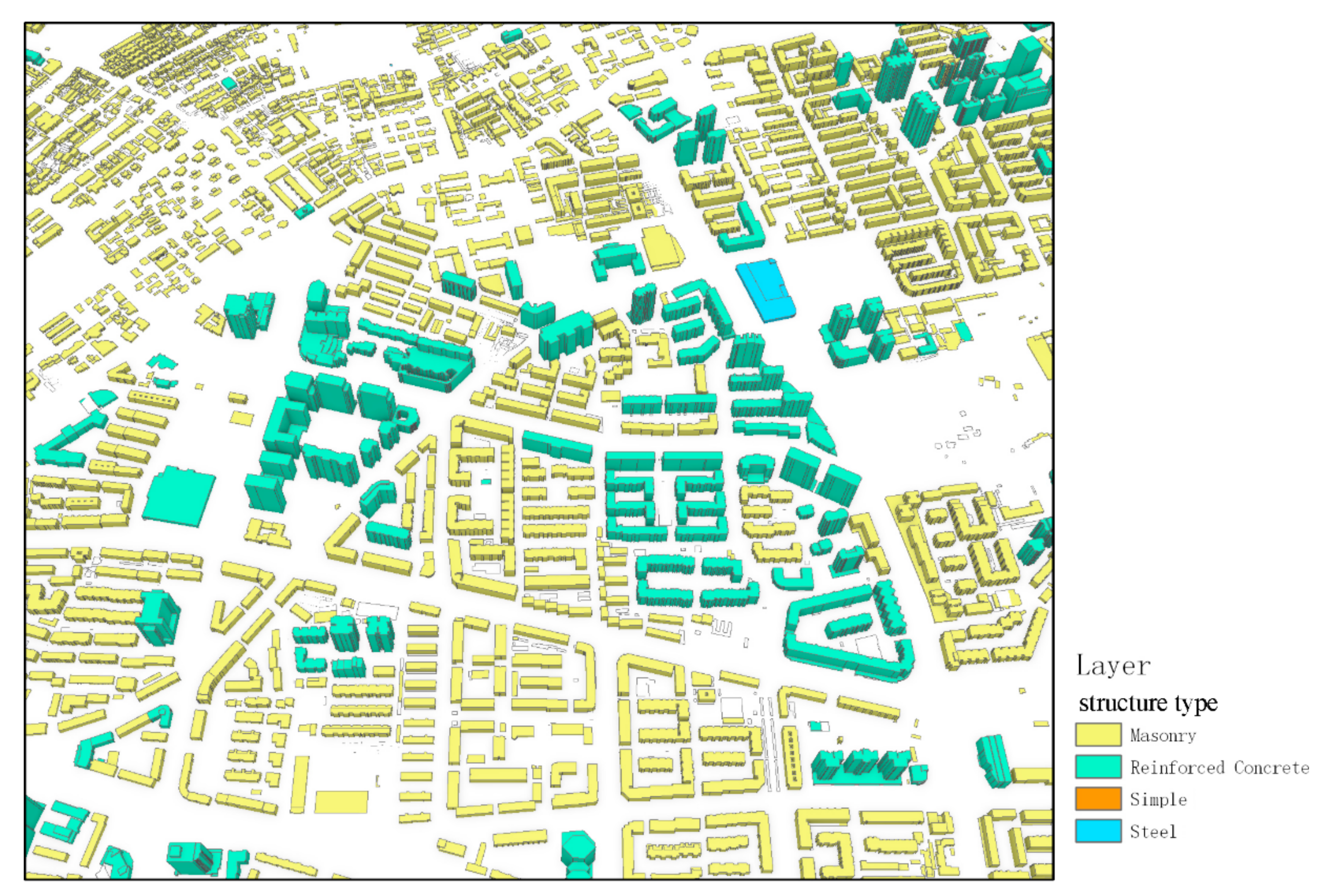
2.5. Vulnerability Classification
2.6. Loss Assessment
2.6.1. Structural Damage
2.6.2. Economic Loss
2.6.3. Social Loss
2.7. Evaluation Indicators
3. Results
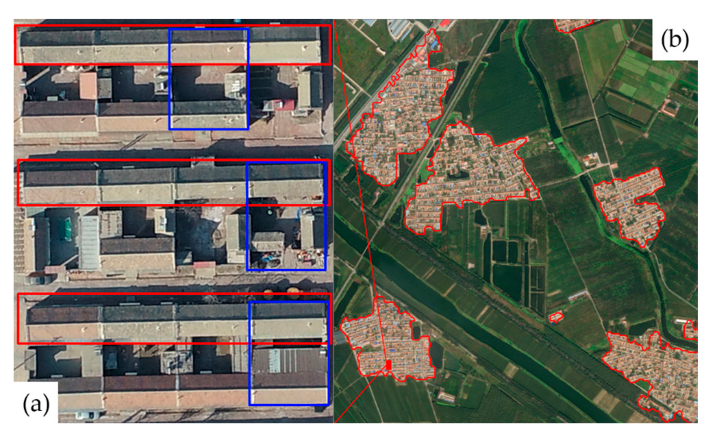
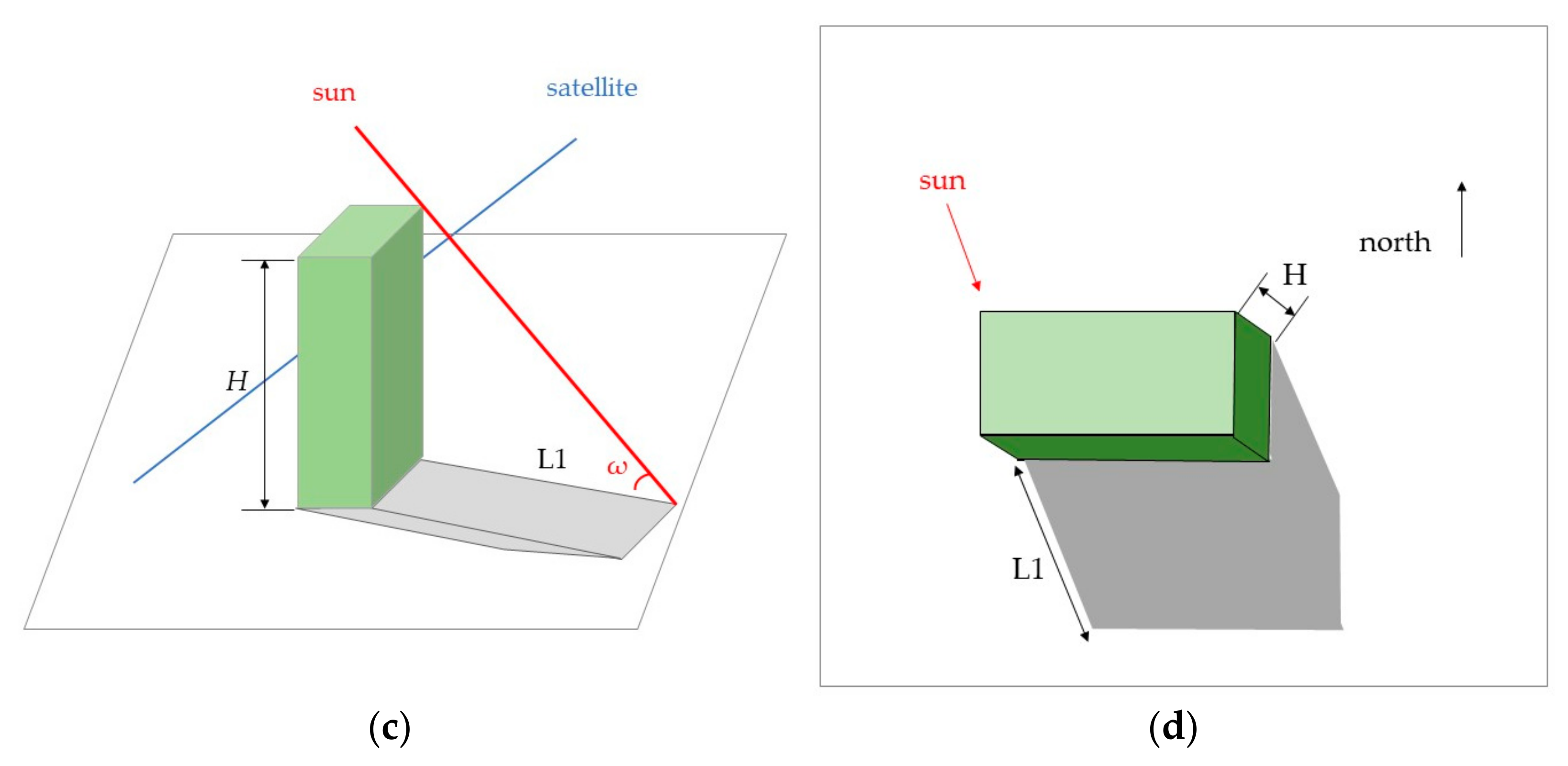
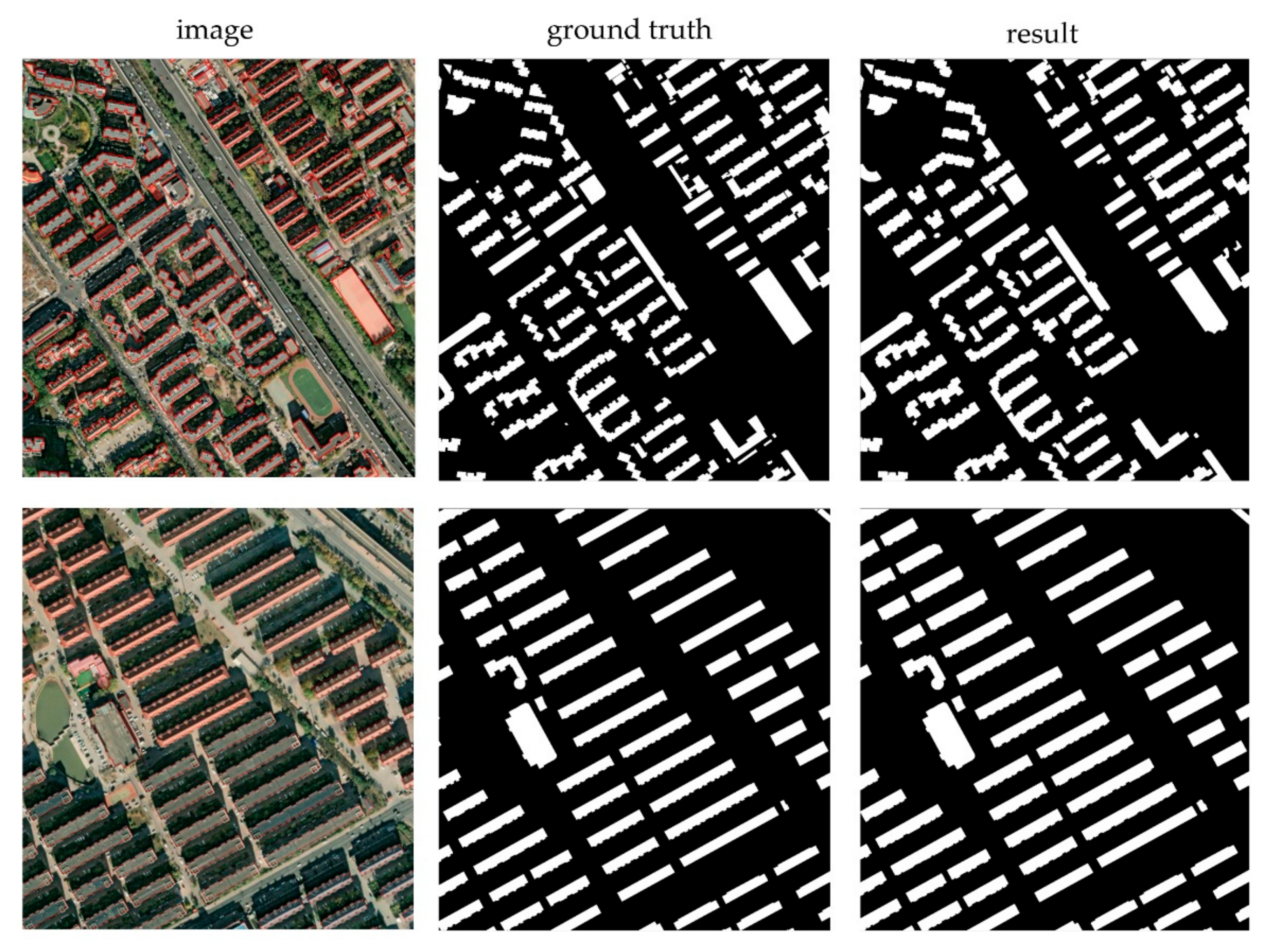
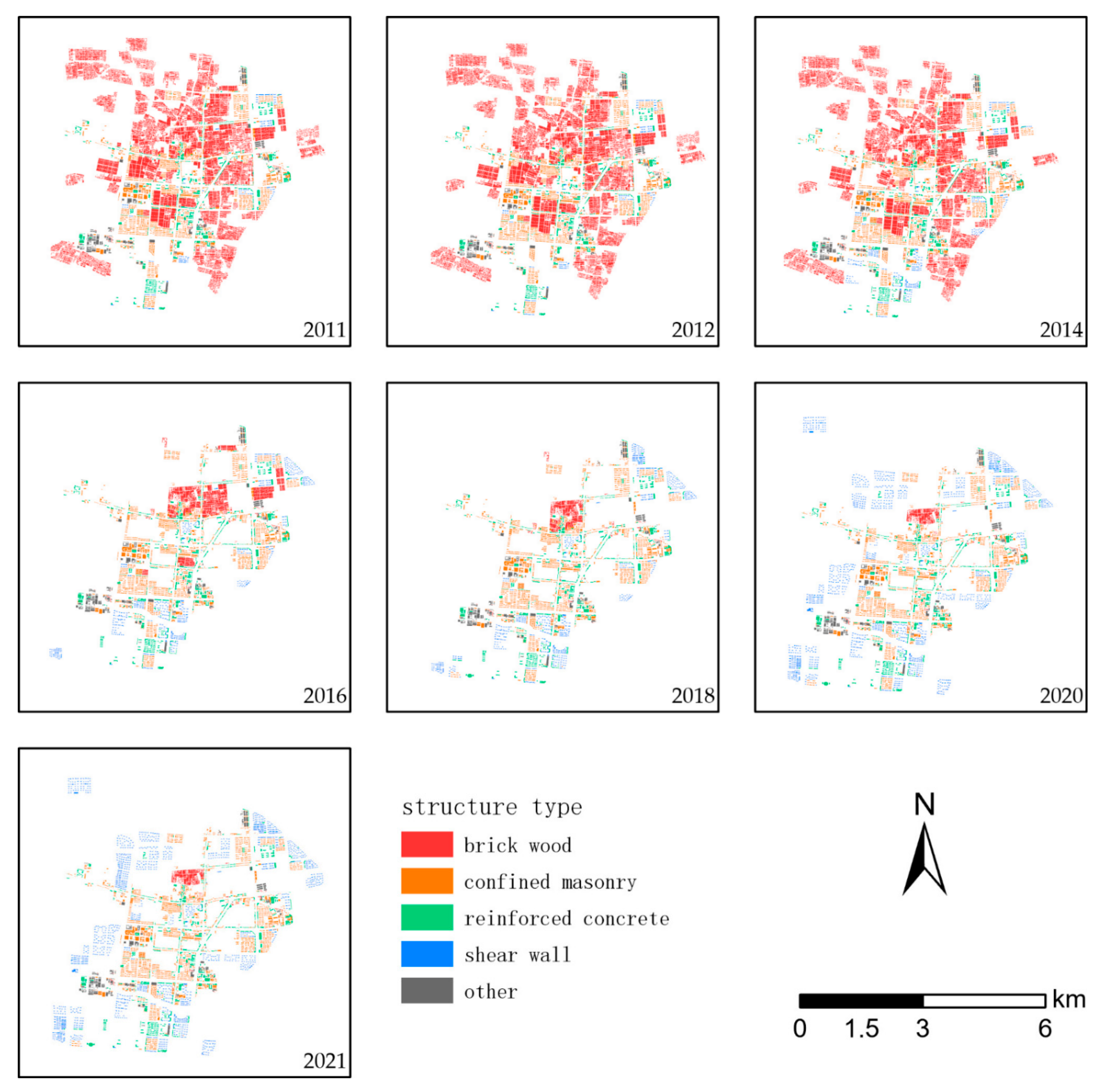
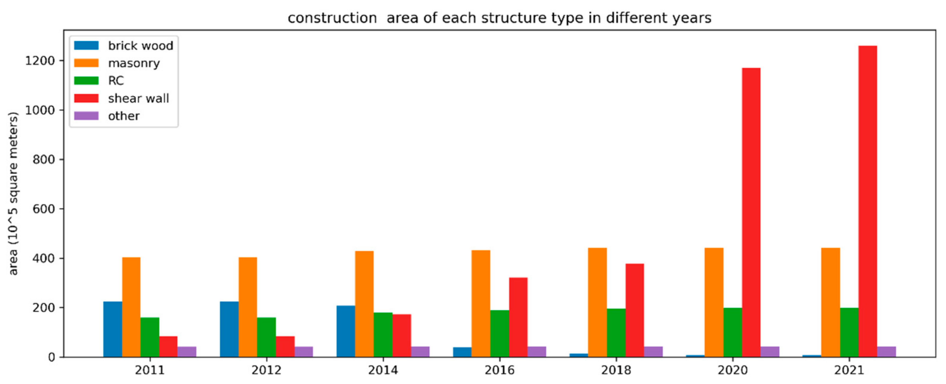
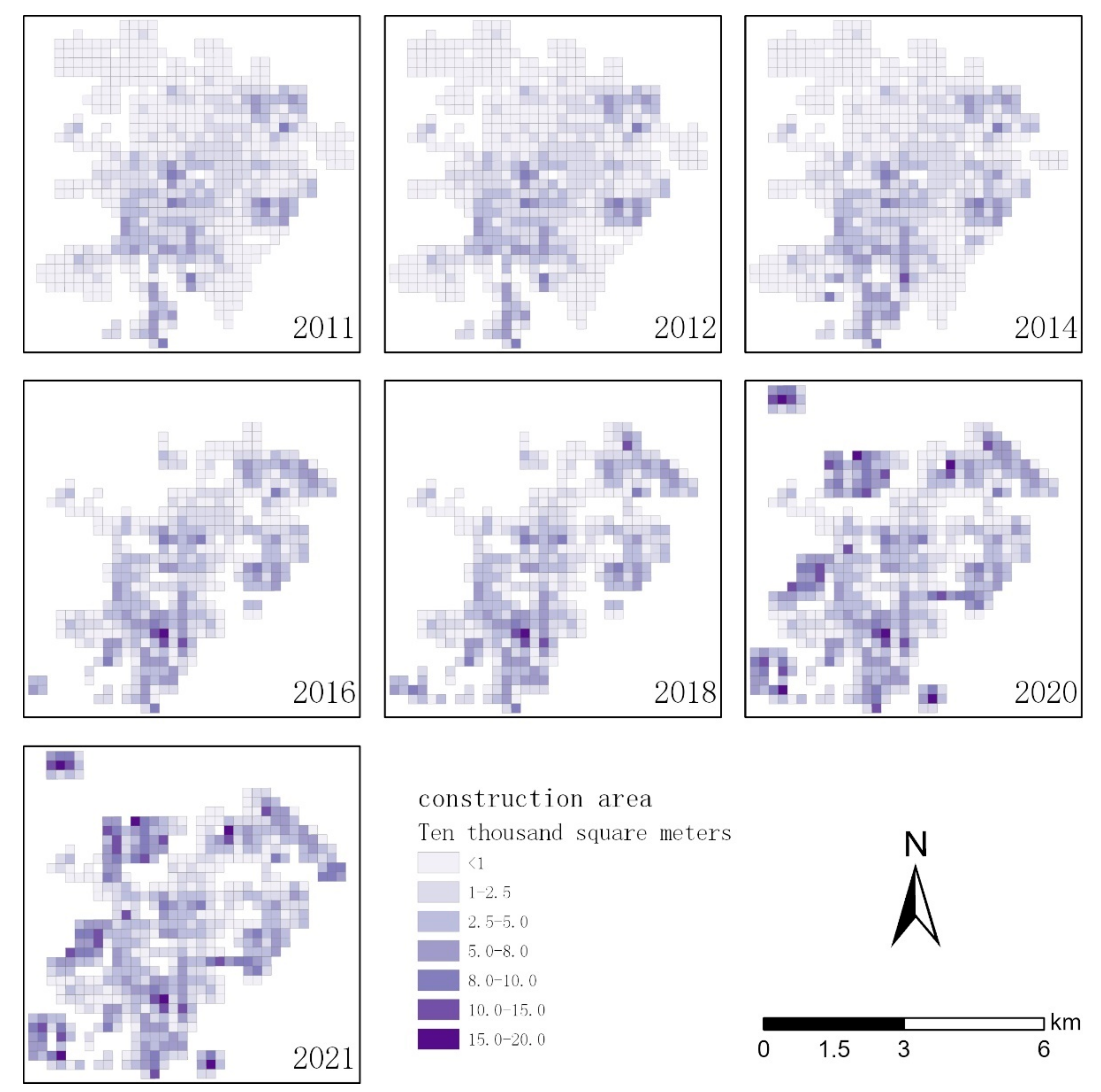
3.1. Building Information Extraction Result
3.2. Estimation of Seismic Risk Changes
4. Discussion
5. Conclusions
Author Contributions
Funding
Institutional Review Board Statement
Informed Consent Statement
Data Availability Statement
Acknowledgments
Conflicts of Interest
References
- Urbanization. Available online: https://en.wikipedia.org/wiki/Urbanization (accessed on 24 March 2022).
- What Should We Understand about Urbanization in China? YALE INSIGHT. 2013. Available online: https://insights.som.yale.edu/insights/what-should-we-understand-about-urbanization-in-china (accessed on 7 March 2022).
- Urbanization and Disaster Risks. Spotlightnepal. Available online: https://www.spotlightnepal.com/2016/01/02/urbanization-and-disaster-risks/ (accessed on 28 April 2022).
- Feng, B.; Zhang, Y.; Bourke, R. Urbanization impacts on flood risks based on urban growth data and coupled flood models. Nat. Hazards 2021, 106, 613–627. [Google Scholar] [CrossRef]
- Global Assessment Report on Disaster Risk Reduction 2015. Available online: https://www.preventionweb.net/english/hyogo/gar/2015/en/home/download.html (accessed on 28 April 2022).
- Earthquakes are the Most Damaging of all Natural Disasters. Available online: https://www.163.com/dy/article/DUSSDFLN0514R9P4.html (accessed on 28 April 2022).
- Chen, Y.; Qi, C. Earthquakes and Seismic Hazard in China. In Science Progress in China; Science Press: Beijing, China, 2003; pp. 387–400. [Google Scholar] [CrossRef]
- China National Earthquake Data Center. Available online: https://data.earthquake.cn/ (accessed on 28 April 2022).
- In Fact, 41% of the Big Cities in China Are in Earthquake-Prone Zone. Available online: https://www.bilibili.com/video/BV1HF411z7Td?share_source=copy_web (accessed on 24 March 2022).
- Wu, J. The direction and path of earthquake disaster risk prevention and control. Overv. Disaster Prev. 2021, 119, 28–31. (In Chinese) [Google Scholar]
- Sendai Framework for Disaster Risk Reduction 2015–2030. Available online: https://www.unisdr.org/files/43291_sendaiframeworkfordrren.pdf (accessed on 24 March 2022).
- Boughazi, K.; Rebouh, S.; Aiche, M.; Harkat, N. Seismic Risk, and Urbanization: The Notion of Prevention. Case of the City of Algiers. Procedia Econ. Financ. 2014, 18, 544–551. [Google Scholar] [CrossRef] [Green Version]
- Vitor, S.; Helen, C.; Marco, P.; Damiano, M.; Rui, P. Development of the OpenQuake engine, the Global Earthquake Model’s open-source software for seismic risk assessment. Nat. Hazards 2014, 72, 1409–1427. [Google Scholar]
- Federal Emergency Management Agency (FEMA)-National Institute of Building Sciences (NIBS). Earthquake Loss Estimation Methodology—HAZUS97; Technical Manual; Federal Emergency Management Agency: Washington, DC, USA, 1970. [Google Scholar]
- Hosseinpour, V.; Saeidi, A.; Nollet, M.-J.; Nastev, M. Seismic loss estimation software: A comprehensive review of risk assessment steps, software development, and limitations. Eng. Struct. 2021, 32, 111866. [Google Scholar] [CrossRef]
- Ghaffarian, S.; Kerle, N.; Filatova, T. Remote Sensing-Based Proxies for Urban Disaster Risk Management and Resilience: A Review. Remote Sens. 2018, 10, 1760. [Google Scholar] [CrossRef] [Green Version]
- Polli, D.; Dell’Acqua, F.; Gamba, P. First steps towards a framework for earth observation (EO)-based seismic vulnerability evaluation. Environ. Semeiot. 2009, 2, 16–30. [Google Scholar] [CrossRef]
- Zhai, Y.M. Research on the Application of High-Resolution Remote Sensing Images in Prediction and Rapid Evaluation of Urban Earthquake Damage. Ph.D. Thesis, Tongji University, Shanghai, China, 2009. (In Chinese). [Google Scholar]
- Borzi, B.; Dell’Acqua, F.; Faravelli, M.; Gamba, P.; Lisini, G.; Onida, M.; Polli, D. Vulnerability study on a large industrial area using satellite remotely sensed images. Bull. Earthq. Eng. 2011, 9, 675–690. [Google Scholar]
- Polli, D.; Dell’Acqua, F. Fusion of optical and SAR data for seismic vulnerability mapping of buildings. In Optical Remote Sensing; Springer: Berlin/Heidelberg, Germany, 2011; pp. 329–341. [Google Scholar]
- Wang, H.F.; Zhai, Y.M.; Chen, X. Rapid Prediction of Earthquake Disaster of Buildings Based on Remote Sensing Images. North China Earthq. Sci. 2010, 28, 45–47. (In Chinese) [Google Scholar]
- Zhao, Q.; Zhai, Y.G.; Li, T.Z. Study on Application of High-Resolution Remote Sensing Images in Rapid Prediction of Earthquake Disaster in Urban Area. J. Catastrophol. 2012, 27, 72–76. (In Chinese) [Google Scholar]
- Ma, J.J.; Feng, Q.M.; Zhou, H.Y. Method for predicting earthquake damage of housing building groups based on image explanation. J. Nat. Disasters 2013, 3, 62–67. (In Chinese) [Google Scholar] [CrossRef]
- Pittore, M.; Wieland, M. Toward a rapid probabilistic seismic vulnerability assessment using satellite and ground-based remote sensing. Nat. Hazards 2013, 68, 115–145. [Google Scholar] [CrossRef]
- Matsuoka, M.; Miura, H.; Midorikawa, S.; Estrada, M. Extraction of urban information for seismic hazard and risk assessment in Lima, Peru using satellite imagery. J. Disaster Res. 2013, 8, 328–345. [Google Scholar]
- Matsuoka, M.; Mito, S.; Midorikawa, S.; Miura, H.; Quiroz, L.G.; Maruyama, Y.; Estrada, M. Development of building inventory data and earthquake damage estimation in Lima, Peru for future earthquakes. J. Disaster Res. 2014, 9, 1032–1041. [Google Scholar] [CrossRef]
- Geiß, C.; Taubenboeck, H.; Tyagunov, S.; Tisch, A.; Post, J.; Lakes, T. Assessment of seismic building vulnerability from space. Earthq. Spectra 2014, 30, 1553–1583. [Google Scholar] [CrossRef]
- Wieland, M.; Pittore, M.; Parola, S.; Begaliev, U.; Yasunov, P.; Tyagunov, S.; Moldobekov, B.; Saidiy, S.; Ilyasov, I.; Abakanov, T. A multiscale exposure model for seismic risk assessment in Central Asia. Seismol. Res. Lett. 2014, 86, 210–222. [Google Scholar] [CrossRef] [Green Version]
- Riedel, I.; Guéguen, P.; Dalla, M.M.; Pathier, E.; Leduc, T.; Chanussot, J. Seismic vulnerability assessment of urban environments in moderate-to-low seismic hazard regions using association rule learning and support vector machine methods. Nat. Hazards 2015, 76, 1111–1141. [Google Scholar] [CrossRef]
- Abruzzese, D.; Angelaccio, M.; Giuliano, R.; Miccoli, L.; Vari, A. Monitoring and vibration risk assessment in cultural heritage via Wireless Sensors Network. In Proceedings of the 2nd Conference on Human System Interactions, Catania, Italy, 21–23 May 2009. [Google Scholar] [CrossRef]
- Ceriotti, M.; Mottola, L.; Picco, G.P.; Murphy, A.L.; Guna, S.; Corra, M.; Pozzi, M.; Zonta, D.; Zanon, P. Monitoring heritage buildings with wireless sensor networks: The Torre Aquila deployment. In Proceedings of the International Conference on Information Processing in Sensor Networks, San Francisco, CA, USA, 13–16 April 2009; pp. 277–288. [Google Scholar]
- Gaudiosi, G.; Alessio, G.; Nappi, R.; Noviello, V.; Spiga, E.; Porfido, S. Evaluation of Damages to the Architectural Heritage of Naples as a Result of the Strongest Earthquakes of the Southern Apennines. Appl. Sci. 2020, 10, 6880. [Google Scholar] [CrossRef]
- Ball, J.; Anderson, D.; Chan, C.S.A. Comprehensive Survey of Deep Learning in Remote Sensing: Theories, Tools, and Challenges for the Community. J. Appl. Remote Sens. 2017, 11, 042609. [Google Scholar] [CrossRef] [Green Version]
- LeCun, Y.; Bottou, L.; Bengio, Y.; Haffner, P. Gradient-Based Learning Applied to Document Recognition. Proc. IEEE 1998, 86, 2278–2324. [Google Scholar] [CrossRef] [Green Version]
- Zhang, L.; Zhang, L.; Du, B. Deep Learning for Remote Sensing Data: A Technical Tutorial on the State of the Art. IEEE Geosci. Remote Sens. Mag. 2016, 4, 22–40. [Google Scholar] [CrossRef]
- Krizhevsky, A.; Sutskever, I.; Hinton, G. ImageNet Classification with Deep Convolutional Neural Networks. Communications of the ACM. 2017, 60, 84–90. [Google Scholar] [CrossRef]
- Simonyan, K.; Zisserman, A. Very deep convolutional networks for large-scale image recognition. In Proceedings of the 3rd International Conference Learn Represent ICLR, San Diego, CA, USA, 7–9 May 2015; pp. 1–14. [Google Scholar] [CrossRef]
- He, K.; Zhang, X.; Ren, S.; Sun, J. Deep Residual Learning for Image Recognition. In Proceedings of the 2016 IEEE Conference on Computer Vision and Pattern Recognition (CVPR), Las Vegas, NV, USA, 27–30 June 2016; pp. 770–778. [Google Scholar] [CrossRef] [Green Version]
- Long, J.; Shelhamer, E.; Darrell, T. Fully convolutional networks for semantic segmentation. In Proceedings of the IEEE Conference on Computer Vision and Pattern Recognition 2015, Boston, MA, USA, 7–12 June 2015; pp. 3431–3440. [Google Scholar]
- Ronneberger, O.; Fischer, P.; Brox, T. U-Net: Convolutional Networks for Biomedical Image Segmentation. In Medical Image Computing and Computer-Assisted Intervention; Springer: Cham, Switzerland, 2015; pp. 234–241. [Google Scholar]
- Badrinarayanan, V.; Kendall, A.; Cipolla, R. SegNet: A Deep Convolutional Encoder-Decoder Architecture for Image Segmentation. IEEE Trans. Pattern Anal. Mach. Intell. 2017, 39, 2481–2495. [Google Scholar] [CrossRef]
- Zhao, H.; Shi, J.; Qi, X.; Wang, X.; Jia, J. Pyramid Scene Parsing Network. In Proceedings of the IEEE Conference on Computer Vision and Pattern Recognition 2017, Honolulu, HI, USA, 21–26 July 2017. [Google Scholar]
- Chen, L.C.; Papandreou, G.; Kokkinos, I.; Murphy, K.; Yuille, A.L. Deeplab:Semantic Image Segmentation with Deep Convolutional Nets, Atrous Convolution, and Fully Connected CRFs. IEEE Trans. Pattern Anal. Mach. Intell. 2018, 40, 834–848. [Google Scholar] [CrossRef] [Green Version]
- Chen, L.C.; Papandreou, G.; Schroff, F.; Adam, H. Rethinking Atrous Convolution for Semantic Image Segmentation. arXiv 2017, arXiv:1706.05587. [Google Scholar]
- Chen, L.-C.; Zhu, Y.-K.; Papandreou, G. Encoder-Decoder with Atrous Separable Convolution for Semantic Image Segmentation. In Proceedings of the European Conference on Computer Vision (ECCV), Munich, Germany, 8–14 September 2018. [Google Scholar]
- Kaiming, H.; Gkioxari, G.; Dollár, P.; Girshick, R. Mask R-CNN. Computer Vision and Pattern Recognition(cs.CV). arXiv 2018, arXiv:1703.06870v3. [Google Scholar]
- Zhan, Y.; Liu, W.; Maruyama, Y. Damaged Building Extraction Using Modified Mask R-CNN Model Using Post-Event Aerial Images of the 2016 Kumamoto Earthquake. Remote Sens. 2022, 14, 1002. [Google Scholar] [CrossRef]
- Altaweel, M.; Khelifi, A.; Li, Z.; Squitieri, A.; Basmaji, T.; Ghazal, M. Automated Archaeological Feature Detection Using Deep Learning on Optical UAV Imagery: Preliminary Results. Remote Sens. 2022, 14, 553. [Google Scholar] [CrossRef]
- Wang, Y.; Li, S.; Teng, F.; Lin, Y.; Wang, M.; Cai, H. Improved Mask R-CNN for Rural Building Roof Type Recognition from UAV High-Resolution Images: A Case Study in Hunan Province, China. Remote Sens. 2022, 14, 265. [Google Scholar] [CrossRef]
- Yu, K.; Hao, Z.; Post, C.J.; Mikhailova, E.A.; Lin, L.; Zhao, G.; Tian, S.; Liu, J. Comparison of Classical Methods and Mask R-CNN for Automatic Tree Detection and Mapping Using UAV Imagery. Remote Sens. 2022, 14, 295. [Google Scholar] [CrossRef]
- Liu, H.; Gong, P.; Wang, J.; Clinton, N.; Bai, Y.; Liang, S. Annual Dynamics of Global Land Cover and its Long-term Changes from 1982 to 2015. Earth Syst. Sci. Data 2020, 12, 1217–1243. [Google Scholar]
- Gong, P.; Li, X.C.; Zhang, W. 40-Year (1978–2017) human settlement changes in China reflected by impervious surfaces from satellite remote sensing. Sci. Bull. 2019, 64, 756–763. [Google Scholar] [CrossRef] [Green Version]
- Yang, J.; Huang, X. The 30 m annual land cover dataset and its dynamics in China from 1990 to 2019. Earth Syst. Sci. Data 2021, 13, 3907–3925. [Google Scholar] [CrossRef]
- Gruenhagen, L.; Juergens, C. Multitemporal Change Detection Analysis in an Urbanized Environment Based upon Sentinel-1 Data. Remote Sens. 2022, 14, 1043. [Google Scholar] [CrossRef]
- Daudt, R.C.; Le Saux, B.; Boulch, A.; Gousseau, Y. Urban change detection for multispectral earth observation using convolutional neural networks. In Proceedings of the IGARSS 2018—2018 IEEE International Geoscience and Remote Sensing Symposium, Valencia, Spain, 22–27 July 2018; pp. 2115–2118. [Google Scholar]
- Huang, X.; Cao, Y.; Li, J. An automatic change detection method for monitoring newly constructed building areas using time-series multi-view high-resolution optical satellite images. Remote Sens. Environ. 2020, 244, 111802. [Google Scholar]
- Du, P.; Hou, X.; Xu, H. Dynamic Expansion of Urban Land in China’s Coastal Zone since 2000. Remote Sens. 2022, 14, 916. [Google Scholar] [CrossRef]
- Huang, X.; Wen, D.; Li, J.; Qin, R. Multi-level monitoring of subtle urban changes for the megacities of China using high-resolution multi-view satellite imagery. Remote Sens. Environ. 2017, 196, 56–75. [Google Scholar]
- Statistical Yearbook of District Baodi. 2021. Available online: http://stats.tj.gov.cn/ (accessed on 9 March 2022). (In Chinese)
- He, Y.J. Study on Pattern of Tianjin Urbanization Since 1990. Ph.D. Thesis, Tianjin University, Tianjin, China, 2012. (In Chinese). [Google Scholar]
- Liu, J.W.; Wang, Z.M.; Xie, F.R. Seismic hazard and risk assessments for Beijing-Tianjin-Tangshan area, China. Chin. J. Geophys. 2010, 53, 318–325. (In Chinese) [Google Scholar] [CrossRef]
- Zhang, H.; Xu, K.; Wang, H.; Pan, Z.; Zhuan, S.P.; Zhang, Y.Q.; Li, Q.Z.; Bu, L.; Shi, G.Y.; Zhang, J.L. Study on the Activity of Baodi Fault Since Late Pleistocene in the Northern Margin of North China Basin. J. Geod. Geodyn. 2021, 41, 1169–1176, 1188. (In Chinese) [Google Scholar]
- WorldPop. Available online: https://www.worldpop.org/project/categories?id=3 (accessed on 24 March 2022).
- Dunbar, P.K.; Bilham, R.G.; Laituri, M.J. Earthquake loss estimation for India based on macroeconomic indicators. In Risk Science and Sustainability; Springer: Dordrecht, Netherlands, 2003; pp. 163–180. [Google Scholar]
- Shaoqing, R.; Kaiming, H.; Ross, G.; Jian, S. Faster R-CNN: Towards Real-Time Object Detection with Region Proposal Networks. IEEE Trans. Pattern Anal. Mach. Intell. 2017, 39, 1137–1149. [Google Scholar] [CrossRef] [Green Version]
- Ross., G. Fast R-CNN. In Proceedings of the 2015 IEEE International Conference on Computer Vision (ICCV), Washington, DC, USA, 7–13 December 2015; pp. 1440–1448. [Google Scholar] [CrossRef]
- Mask-Rcnn. Available online: https://ztlevi.github.io/Gitbook_Machine_Learning_Questions/cv/two-stage-detector/mask-rcnn.html (accessed on 24 March 2022).
- Cheng, T.; Wang, X.; Huang, L.; Liu, W. Boundary-preserving Mask R-CNN. In Computer Vision—ECCV 2020; Springer: Cham, Switzerland, 2020. [Google Scholar] [CrossRef]
- Milletari, F.; Navab, N.; Ahmadi, S. V-net: Fully convolutional neural networks for volumetric medical image segmentation. In Proceedings of the 2016 Fourth International Conference on 3D Vision (3DV), Stanford, CA, USA, 25–28 October 2016; pp. 565–571. [Google Scholar]
- Chen, C.; Yang, Z.Y.; Shi, X.L.; Shang, Y. Inversion of urban building height based on Google Earth remote sensing images. Bull. Surv. Mapp. 2020, 1, 90–101. (In Chinese) [Google Scholar] [CrossRef]
- Ecognition. Available online: https://geospatial.trimble.com/products-and-solutions/trimble-ecognition (accessed on 24 March 2022).
- Breiman, L. Random Forests. Mach. Learn. 2001, 45, 5–32. [Google Scholar] [CrossRef] [Green Version]
- Shinozuka, M.; Feng, M.Q.; Lee, J.; Naganuma, T. Statistical Analysis of Fragility Curves. J. Eng. Mech.-Asce. 2000, 126, 1224–1231. [Google Scholar] [CrossRef] [Green Version]
- Yao, X.Q. Analysis of Tianjin Rural Residential Vulnerability and Seismic Capacity Distribution. Ph.D. Thesis, Institute of Engineering Mechanics, China Earthquake Administration, Harbin, China, 2016. (In Chinese). [Google Scholar]
- Xin, D.; Daniell, J.E.; Wenzel, F. State of the art of fragility analysis for major building types in China with implications for intensity-PGA relationships. Nat. Hazards Earth Syst. Sci. Discuss. 2018, 1–34. [Google Scholar] [CrossRef] [Green Version]
- Cui, M.Z.; Wang, C.K.; Chen, C.H.; Pan, Y.H.; Xiong, Y.H.; Ren, C.C. Seismic fragility analysis on existing high-rise shear-wall structure based on incremental dynamic analysis. Build. Sci. 2021, 37, 151–157. [Google Scholar] [CrossRef]
- China Earthquake Administration. GB/T18208.4-2011; Post-Earthquake Field Works—Part 4: Assessment of Direct Loss; Earthquake Press: Beijing, China, 2011. [Google Scholar]
- Kappa_Coefficient. Available online: https://www.tutorialspoint.com/statistics/cohen_kappa_coefficient.htm (accessed on 24 March 2022).
- Wyss, M.; Rosset, P. Near-Real-Time Loss Estimates for Future Italian Earthquakes Based on the M6.9 Irpinia Example. Geosciences 2020, 10, 165. [Google Scholar] [CrossRef]
- Van Houtte, C.; Abbott, E. OpenQuake Implementation of the Canterbury Seismic Hazard Model. Seismol. Res. Lett. 2019, 90, 2227–2235. [Google Scholar] [CrossRef]
- Feliciano, D.; Arroyo, O.; Cabrera, T.; Contreras, D.; Valcárcel Torres, J.A.; Gómez Zapata, J.C. Seismic risk scenarios for the residential buildings in the Sabana Centro province in Colombia. Nat. Hazards Earth Syst. Sci. 2022. (in review). [Google Scholar] [CrossRef]
- Global Assessment Report on Disaster Risk Reduction 2022. Available online: https://www.undrr.org/publication/global-assessment-report-disaster-risk-reduction-2022 (accessed on 28 April 2022).


| Dataset | Source | Spatial Resolution | Time Scale |
|---|---|---|---|
| GF-1/6 | China Center For Resources Satellite Data and Application http://36.112.130.153:7777/DSSPlatform/index.html (accessed on 9 March 2022) | 2 m/8 m | 2014–2020 |
| GF-2 | 1 m/4 m | 2016–2021 | |
| ZY-3 | 2 m/6 m | 2012–2016 | |
| Sentinel 2 | https://scihub.copernicus.eu/ (accessed on 9 March 2022) | 10 m | 2015–2021 |
| Point of interest | https://lbsyun.baidu.com/ (accessed on 9 March 2022) | - | 2018, 2020 |
| Questionnaire | Field survey | - | 2019 |
| Statistical Yearbook | http://stats.tj.gov.cn/ (accessed on 9 March 2022) | - | 2011–2021 |
| Census data | http://stats.tj.gov.cn/ (accessed on 9 March 2022) | - | 2010, 2020, 2021 |
| Occupancy | Office | Factory | Business | Education | Medical | Residency | Other |
|---|---|---|---|---|---|---|---|
| Day | 0.03 | 0.01 | 0.09 | 0.52 | 0.3 | 0.01 | 0.03 |
| Night | 0.001 | 0 | 0 | 0.12 | 0.1 | 0.033 | 0.001 |
| Type | Features | Data |
|---|---|---|
| Extend | Area, length, length/width, width, border length | VHR image |
| Shape | Asymmetry, compactness, density, elliptic fit, rectangular fit, main direction, shape index, roundness | |
| Texture | GLCM (homogeneity, contrast, dissimilarity, entropy, Ang. 2nd moment, mean, Std.Dev.) | Multi-Spectral Data |
| Layer Values | mean, standard deviation, HSI transformation |
| Typology | LS1 | LS2 | LS3 | LS4 | Source | ||||
|---|---|---|---|---|---|---|---|---|---|
| µ | σ | µ | σ | µ | σ | µ | σ | ||
| Brick wood | 0.2997 | 0.093 | 0.2005 | 0.1397 | 0.216 | 0.2175 | 0.2228 | 0.2837 | [74] |
| Confined masonry | 0.139 | 0.845 | 0.292 | 0.709 | 0.510 | 0.608 | 1.372 | 0.828 | [75] |
| Reinforced concrete | 0.267 | 0.785 | 0.540 | 0.548 | 0.841 | 0.506 | 1.629 | 0.558 | [75] |
| shear wall | 0.130 | 0.170 | 0.150 | 0.240 | 0.20 | 0.470 | 0.250 | 0.810 | [76] |
| Bottom RC | 0.122 | 0.2 | 0.145 | 0.2 | 0.213 | 0.2 | 0.461 | 0.2 | [75] |
| Casualty Rate | Moderate Damage | Severely Damaged | Destroyed |
|---|---|---|---|
| Death Rate | 0.001% | 0.5% | 3% |
| Injury Rate | 10% | 15% | 30% |
| Buildings | IoU | Precision | Recall | F1 Score |
|---|---|---|---|---|
| Rural building group | 0.792079 | 0.898876 | 0.869565 | 0.883978 |
| Single buildings | 0.855615 | 0.924855 | 0.91954 | 0.92219 |
| Year | 2011 | 2012 | 2014 | 2016 | 2018 | 2020 | 2021 |
|---|---|---|---|---|---|---|---|
| Day | 240,344 | 240,260 | 258,043 | 268,555 | 274,613 | 360,118 | 369,280 |
| Night | 203,244 | 203,182 | 233,786 | 230,443 | 241,556 | 477,837 | 505,323 |
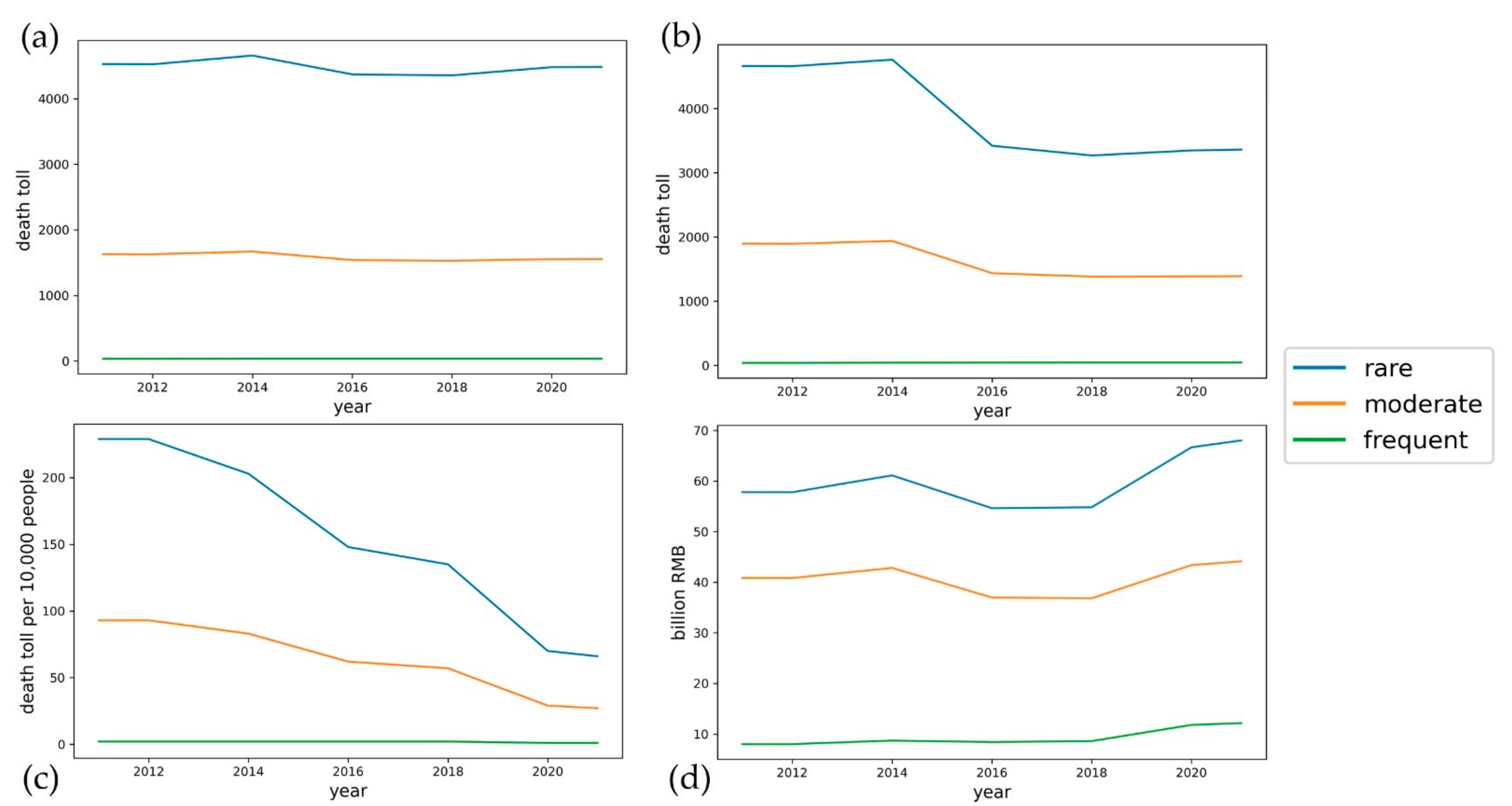
| Level | Year | 2011 | 2012 | 2014 | 2016 | 2018 | 2020 | 2021 |
|---|---|---|---|---|---|---|---|---|
| Rare | Eco loss (billion RMB) | 57.7964 | 57.7817 | 61.1094 | 54.6339 | 54.8115 | 66.6552 | 68.0225 |
| Night death toll | 4662 | 4660 | 4762 | 3421 | 3270 | 3348 | 3362 | |
| Day death toll | 4526 | 4524 | 4658 | 4371 | 4355 | 4480 | 4484 | |
| Moderate | Eco loss (billion RMB) | 40.8394 | 40.8280 | 42.8254 | 36.9838 | 36.8194 | 43.3709 | 44.1346 |
| Night death toll | 1896 | 1895 | 1939 | 1437 | 1384 | 1388 | 1390 | |
| Day death toll | 1630 | 1629 | 1670 | 1540 | 1530 | 1554 | 1555 | |
| Frequent | Eco loss (billion RMB) | 8.0140 | 8.0123 | 8.7140 | 8.4178 | 8.6097 | 11.8013 | 12.1698 |
| Night death toll | 40 | 40 | 43 | 44 | 45 | 45 | 45 | |
| Day death toll | 35 | 35 | 37 | 37 | 37 | 37 | 37 |
Publisher’s Note: MDPI stays neutral with regard to jurisdictional claims in published maps and institutional affiliations. |
© 2022 by the authors. Licensee MDPI, Basel, Switzerland. This article is an open access article distributed under the terms and conditions of the Creative Commons Attribution (CC BY) license (https://creativecommons.org/licenses/by/4.0/).
Share and Cite
An, L.; Zhang, J. Impact of Urbanization on Seismic Risk: A Study Based on Remote Sensing Data. Sustainability 2022, 14, 6132. https://doi.org/10.3390/su14106132
An L, Zhang J. Impact of Urbanization on Seismic Risk: A Study Based on Remote Sensing Data. Sustainability. 2022; 14(10):6132. https://doi.org/10.3390/su14106132
Chicago/Turabian StyleAn, Liqiang, and Jingfa Zhang. 2022. "Impact of Urbanization on Seismic Risk: A Study Based on Remote Sensing Data" Sustainability 14, no. 10: 6132. https://doi.org/10.3390/su14106132