Developing a Hybrid Approach Based on Analytical and Metaheuristic Optimization Algorithms for the Optimization of Renewable DG Allocation Considering Various Types of Loads

Abstract

The optimal location of renewable distributed generations (DGs) into a radial distribution system (RDS) has attracted major concerns from power system researchers in the present years. The main target of DG integration is to improve the overall system performance by minimizing power losses and improving the voltage profile. Hence, this paper proposed a hybrid approach between an analytical and metaheuristic optimization technique for the optimal allocation of DG in RDS, considering different types of load. A simple analytical technique was developed in order to determine the sizes of different and multiple DGs, and a new efficient metaheuristic technique known as the Salp Swarm Algorithm (SSA) was suggested in order to choose the best buses in the system, proportionate to the sizes determined by the analytical technique, in order to obtain the minimum losses and the best voltage profile. To verify the power of the proposed hybrid technique on the incorporation of the DGs in RDS, it was applied to different types of static loads; constant power (CP), constant impedance (CZ), and constant current (CI). The performance of the proposed algorithm was validated using two standards RDSs—IEEE 33-bus and IEEE 69-bus systems—and was compared with other optimization techniques.

1. Introduction

The electric power distribution network is the part which connects the high voltage (HV) electric power transmission network to low voltage (LV) consumers, which is considered the substantial part of the electric power network because the power delivered from the electric power to the loads is assured by operative and reliable distribution networks. The electric power system is sectioned into three parts: generation, transmission, and the distribution network. The last part is the distribution network, which is used to link between the consumers and transmission. The electric power system suffers from two important factors: a low voltage profile and a high percentage of power losses. However, 70% of the power losses are caused at the distribution level (primary and secondary), and the remaining 30% are caused by the transmission system [1]. Hence, the distribution networks attract the main attention of the researchers.

Exiting grids are mostly characterized by centralized bulk power generation far from load centers, requiring long, costly, and lossy transmission lines for power delivery.

By incorporating distribution generation (DG) units in the radial distribution system (RDS) at appropriate places, the losses can reach the minimum value. DG is known as electricity generation by specific capacity generators associated with the electric distribution system or close to the loads.

In smart networks, there is intense interest in the distribution systems to increase the penetration levels of renewable energy sources that are incorporated close to the point-of-use, which achieve lower losses in energy delivery, and this makes the transactions of the power in the lines of the distribution system bidirectional [2].

Research has demonstrated that the incorporation of DG sources in the electric power distribution networks could create various benefits; some of them are:

• Improved voltages of all busses.
• Decreased power losses.
• Improved security of critical buses.
• Network reinforcement.
• The reduction of the congestion of the distribution system.
• The reduction of operation costs.
• The improvement of system reliability

It is very important to incorporate an auxiliary power system beside the main generation in order to supply the loads with sufficient energy. Hence, the electrical network must achieve reliability, which is defined as the probability of this network to perform its intended function for a specific time [3].

In order to achieve these objectives, it is necessary to specify the optimal sizes and location of DG units in distribution systems; otherwise, it could lead to reverse actions, such as the increase in active power losses and a poor voltage profile.

There are multiple types of DGs, which can be discussed as follows:

• Type I: injects only active power, with a unity power factor.
• Type II: injects only reactive power, with zero power factor.
• Type III: injects active and reactive power.
• Type IV: injects active power and consumes reactive power.

Different techniques have been obtained in order to solve the optimization problems: analytical optimization techniques which based on the mathematical model (such as [4,5]) and metaheuristic techniques such as the Ant lion optimization algorithm [6], Hybrid particle swarm optimization, and the Genetic algorithm (GA-PSO) based on active power losses [7,8]; the Artificial Bee Colony Algorithm (ABC) [9]; the Modified Teaching–Learning-Based Optimization algorithm (MTLBO) [10]; and the Harmony Search Algorithm (HSA) [11]. In [12,13], the researchers used a hybrid evolutionary algorithm to specify the optimal DG placement; the improvement of the voltage profile and voltage stability were the main objectives of the researchers in [14,15]. There are also the Whale Optimization Algorithm (WOA) [16] and the Intersect Mutation Differential Evolution optimizer (IMDE) [17].

The loads of the electric distribution system are permanently changing due to consumer demand variations. In industrial areas, the electric power distribution network is susceptible to voltage collapse due to grievous loading conditions.

In load flow studies, it is acceptable to symbolize the composite load properties, as signified from the power given points. In the transmission networks, because of the voltage regulation, the load can be represented by using a constant power model, while in the distribution networks, the voltage is changed along the network lines because most of the buses are not voltage controlled. As such, the properties of the loads in the distribution network analysis are very important and serious.

Distribution power flow studies have been extremely influenced by load modeling. Furthermore, the load characteristics have a noticeable influence on power flow solutions and convergence ability [18].

There are two important types of load: static and dynamic loads. The dynamic loads are not signifying in power flow studies, while static load modeling expresses the active and reactive power as a function of the voltage magnitude of each bus, so it is appropriate for power flow studies, which are in turn categorized into different types of loads, as follows: constant power (CP), constant current (CI), and constant impedance (CZ).

Multiple papers have studied the effect of the DG units in RDS by considering the static load model [19,20]. In order to check the performance of the hybrid technique in power loss reduction and voltage improvement, it is applied to the three types of static loads.

In this paper, a hybrid analytical and metaheuristic technique is proposed in order to calculate the optimal allocation and sizing of multiple types of DGs with different types of load; the analytical technique was proposed to specify the proper size, while the Salp Swarm Algorithm (SSA) was chosen to specify best locations.

SSA is a new efficient optimization algorithm introduced by Mirjalil in 2017 [21]. The behavior of salps in a swarm for foraging or traveling across oceans is the main inspiration of this technique. Salps are a kind of Salpidae family that have a transparent barrel-shaped body; their tissues are highly similar to a jellyfish’s structure. The main reason for this behavior of salps in swarms is unclear as yet, but some of the researchers believe that the swarming is performed in order to achieve the best movement using rapid coordinated alterations and foraging.

The SSA technique is simple and uncomplicated to implement, and includes one controlling parameter C_1; the acclimated mechanism of this algorithm allows it to alert solutions, and ultimately finds an exact estimation of the optimal solutions. The SSA gives strongly satisfying results when it is integrated with other techniques; it is also characterized by its speed in convergence, and is suitable for different optimization problems, while the GA is easy to understand, and deals with multi objective optimization, but one of its important disadvantages is being time consuming and computationally expensive. As such, due to these advantages, SSA is an efficient and excellent technique comparable with recent techniques; nevertheless, this cannot be ensured for all optimization problems. Additionally, the SSA has been used to solve single-objective functions in various optimization areas; the Chaotic Salp Swarm Algorithm (CSSA) is a new optimization technique which was introduced by Sayed et al. [22]. In addition, SSA has been utilized in electrical power engineering problems; in [23], El-Fergany proposed a technique to define the parameters of the polarization curves of polymer exchange membrane fuel cells (PEMFC), which are based on SSA, and in [24], the authors presented a modification and application of SSA called the enhanced salp swarm algorithm (ESSA); in [25], the SSA was employed to solve optimal power flow (OPF) problems.

The rest of the paper is sectioned as follows: the problem formulation, including the load modeling, forward/backward load flow algorithm, objective function, and operational constraints are illustrated in Section 2; the SSA is presented in Section 3; Section 4 illustrates the analytical technique; Section 5 presents the simulation results; finally, the conclusion of the paper is illustrated in Section 6.

2. Problem Formulation

2.1. Load Modelling

In this paper, three types of static loads are studied, as follows:

• Constant impedance (CZ): the power is proportional to the square of the voltage value.
• Constant current (CI): the power is proportional to the voltage value.
• Constant power (CP): the power does not change with the voltage variation.

In this article, the exponential form is used to define the static load as follows:

$${\mathrm{P}}_{\mathrm{A}}={\mathrm{P}}_{0_{\mathrm{A}}}{\ast \mathrm{V}}_{\mathrm{A}}{}^{\mathsf{\sigma }}$$

(1)

$${\mathrm{Q}}_{\mathrm{A}}={\mathrm{Q}}_{0_{\mathrm{A}}}{\ast \mathrm{V}}_{\mathrm{A}}{}^{\mathsf{\sigma }}$$

(2)

where ${\mathrm{P}}_{\mathrm{A}}{\mathrm{and}\mathrm{Q}}_{\mathrm{A}}$ are the active and reactive power at bus$\mathrm{A}$, $\mathrm{V}$ is the voltage magnitude at bus $\mathrm{A}$,$\mathsf{\sigma }=0$ at constant power (CP),$\mathsf{\sigma }=1$ at constant current (CI), and $\mathsf{\sigma }=2$ at constant impedance (CZ).

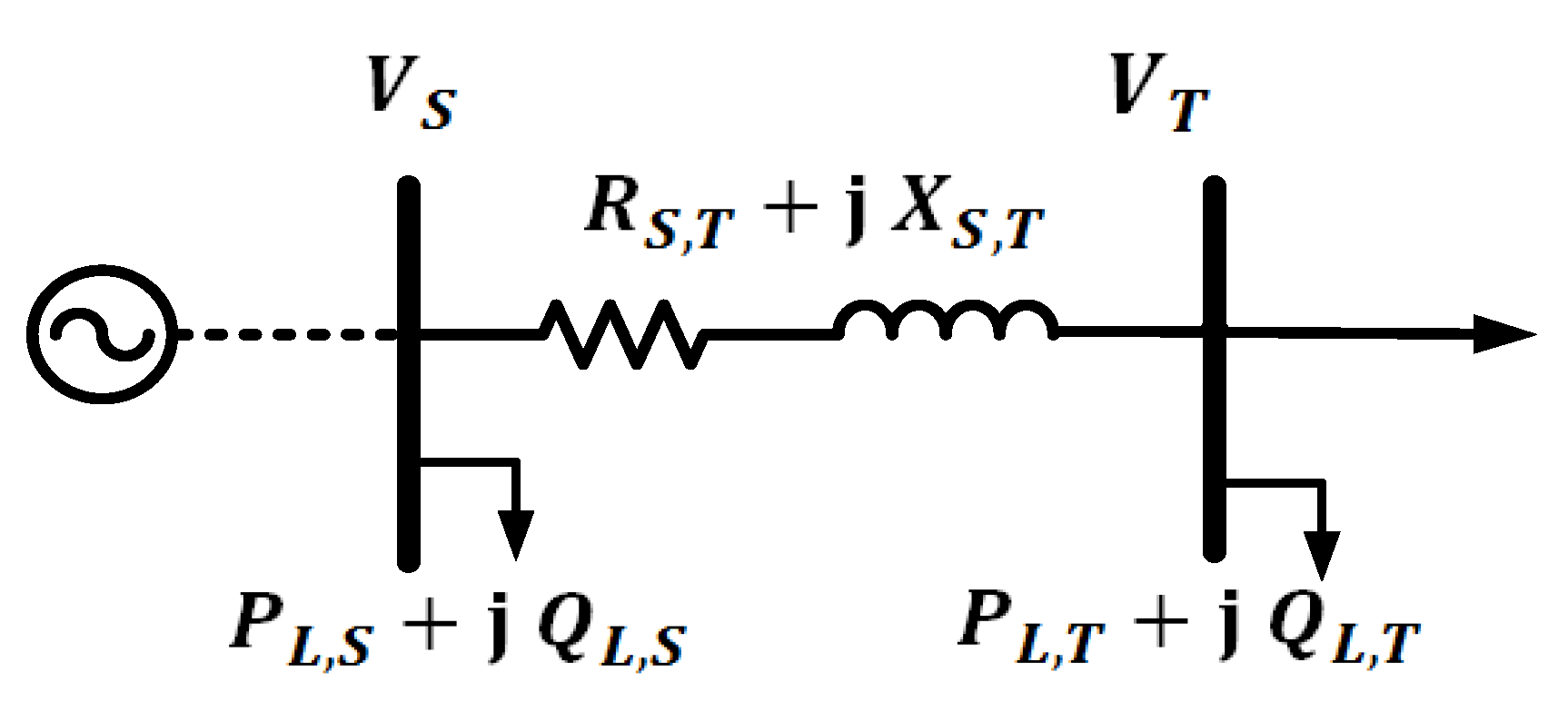
2.2. Forward–Backward Power Flow Algorithm

RDSs have some special properties, such as a radial structure, a high R/X ratio, and unbalanced loads. Due to the previous features, Gauss–Seidel (GS), Newton Raphson (NR), and the fast decoupled method are inefficient in radial distribution system analysis. Hence, the forward–backward load flow is a modern technique which is used in this paper to solve the load flow in RDS, which is divided into two processes: forward sweep and backward sweep. The voltage in the forward sweep is calculated from sending to the end of the feeder, while the power in the backward sweep is calculated from the end of the feeder to the source. Figure 1 illustrates two bus RDS; the active power P_S and the reactive power Q_S that flow from bus S to T can be calculated from backward sweep as follows.

$${\mathrm{P}}_{\mathrm{S}}={\mathrm{P}}_{\mathrm{T}}+{\mathrm{P}}_{\mathrm{L},\mathrm{T}}+\mathrm{R}\left(\frac{{({\mathrm{P}}_{\mathrm{T}}+{\mathrm{P}}_{\mathrm{L},\mathrm{T}})}^2+{({\mathrm{Q}}_{\mathrm{T}}+{\mathrm{Q}}_{\mathrm{L},\mathrm{T}})}^2}{{\left|{\mathrm{V}}_{\mathrm{T}}\right|}^2}\right).$$

(3)

$${\mathrm{Q}}_{\mathrm{S}}={\mathrm{Q}}_{\mathrm{T}}+{\mathrm{Q}}_{\mathrm{L},\mathrm{T}}+\mathrm{X}\left(\frac{{({\mathrm{P}}_{\mathrm{T}}+{\mathrm{P}}_{\mathrm{L},\mathrm{T}})}^2+{({\mathrm{Q}}_{\mathrm{T}}+{\mathrm{Q}}_{\mathrm{L},\mathrm{T}})}^2}{{\left|{\mathrm{V}}_{\mathrm{T}}\right|}^2}\right)$$

(4)

and the voltage of each bus can be determined in the forward sweep as:

$${\mathrm{V}}_{\mathrm{T}}^2=\left({\mathrm{V}}_{\mathrm{S}}^2-2\left({\mathrm{P}}_{\mathrm{S}}\mathrm{R}+{\mathrm{Q}}_{\mathrm{S}}\mathrm{X}\right)+\left({\mathrm{R}}^2+{\mathrm{X}}^2\right)\frac{\left({\mathrm{P}}_{\mathrm{S}}{}^2+{\mathrm{Q}}_{\mathrm{S}}{}^2\right)}{{\mathrm{V}}_{\mathrm{S}}^2}\right)$$

(5)

therefore, the active power loss in the branch from $\mathrm{S}$ to $\mathrm{T}$ can be determined as:

$${\mathrm{P}}_{\mathrm{loss}\left(\mathrm{S},\mathrm{T}\right)}={\mathrm{R}}_{\mathrm{S},\mathrm{T}}\left(\frac{{\mathrm{P}}_{\mathrm{S}}^2+{\mathrm{jQ}}_{\mathrm{S}}^2}{{\left|{\mathrm{V}}_{\mathrm{S}}\right|}^2}\right)$$

(6)

and the reactive power loss in the branch from S to T can be determined as:

$${\mathrm{Q}}_{\mathrm{loss}\left(\mathrm{S},\mathrm{T}\right)}={\mathrm{x}}_{\mathrm{S},\mathrm{T}}\left(\frac{{\mathrm{P}}_{\mathrm{S}}^2+{\mathrm{jQ}}_{\mathrm{S}}^2}{{\left|{\mathrm{V}}_{\mathrm{S}}\right|}^2}\right)$$

(7)

Hence, the total active and reactive power losses in RDS can be estimated as:

$$\mathrm{TPL}={\displaystyle \sum }_{\mathrm{s},\mathrm{t}=1}^{\mathrm{Br}}\left({\mathrm{P}}_{\mathrm{Loss}}\left(\mathrm{S},\mathrm{T}\right)\right)$$

(8)

$$\mathrm{TQL}={\displaystyle \sum }_{\mathrm{s},\mathrm{t}=1}^{\mathrm{Br}}\left({\mathrm{Q}}_{\mathrm{Loss}}\left(\mathrm{S},\mathrm{T}\right)\right)$$

(9)

2.3. Objective Function

In general, incorporating DGs into RDS reduces the power losses by reducing the amount of current flowing in the lines; also, it can improve the overall voltage profile, which in turn improves the efficiency of the network.

In the present work, the main objective function is to minimize total active power losses. Therefore, the objective function can be formulated as:

$${\mathrm{P}}_{\mathrm{Loss}}={\displaystyle \sum }_{\mathrm{S}=1}^{\mathrm{No}}{\displaystyle \sum }_{\mathrm{T}=1}^{\mathrm{No}}{\mathsf{\alpha }}_{\mathrm{ST}}\left({\mathrm{P}}_{\mathrm{S}}{\mathrm{P}}_{\mathrm{T}}+{\mathrm{Q}}_{\mathrm{S}}{\mathrm{Q}}_{\mathrm{T}}\right)+{\mathsf{\beta }}_{\mathrm{ST}}\left({\mathrm{Q}}_{\mathrm{S}}{\mathrm{P}}_{\mathrm{T}}-{\mathrm{P}}_{\mathrm{S}}{\mathrm{Q}}_{\mathrm{T}}\right)$$

(10)

${\mathrm{P}}_{\mathrm{S}}{\mathrm{and}\mathrm{P}}_{\mathrm{T}}$ are the active power at bus $\mathrm{S}\mathrm{and}\mathrm{T}$, respectively

${\mathrm{Q}}_{\mathrm{S}}{\mathrm{and}\mathrm{Q}}_{\mathrm{T}}$ are the reactive power at bus $\mathrm{S}\mathrm{and}\mathrm{T}$, respectively.

2.4. Operation Constraints

2.4.1. Equality Constraints

$${\mathrm{P}}_{\mathrm{Slack}}+{\displaystyle \sum }_{\mathrm{A}}^{\mathrm{No}}{\mathrm{P}}_{\mathrm{DG}\left(\mathrm{A}\right)}={\displaystyle \sum }_{\mathrm{A}}^{\mathrm{No}}{\mathrm{P}}_{\mathrm{Load}\left(\mathrm{A}\right)}+{\displaystyle \sum }_{\mathrm{B}}^{\mathrm{Br}}{\mathrm{P}}_{\mathrm{Loss}\left(\mathrm{B}\right)}$$

(11)

$${\mathrm{Q}}_{\mathrm{Slack}}+{\displaystyle \sum }_{\mathrm{A}}^{\mathrm{No}}{\mathrm{Q}}_{\mathrm{DG}\left(\mathrm{A}\right)}={\displaystyle \sum }_{\mathrm{A}}^{\mathrm{No}}{\mathrm{Q}}_{\mathrm{Load}\left(\mathrm{A}\right)}+{\displaystyle \sum }_{\mathrm{B}}^{\mathrm{Br}}{\mathrm{Q}}_{\mathrm{Loss}\left(\mathrm{B}\right)}$$

(12)

${\mathrm{P}}_{\mathrm{Slack},} {\mathrm{Q}}_{\mathrm{Slack}}$ are the active and reactive power of the slack bus, respectively.

No: number of buses; Br: number of branches$;{\mathrm{P}}_{\mathrm{Loss}}$: active power loss.

2.4.2. Inequality Constraints

The voltage at each bus must be between 0.90 and 1.05.

$${\mathrm{V}}_{\min }\le {\mathrm{V}}_{\mathrm{A}}\le {\mathrm{V}}_{\max }$$

(13)

The total reactive power injected by the DG is less than the total reactive power of loads.

$${{\displaystyle \sum }}^{\text{}}{\mathrm{Q}}_{\mathrm{DG}}\le {\displaystyle \sum }_{\mathrm{A}}^{\mathrm{No}}{\mathrm{Q}}_{\mathrm{Load}\left(\mathrm{A}\right)}$$

(14)

The total active power injected by the DG is less than the total active power loads.

$${{\displaystyle \sum }}^{\text{}}{\mathrm{P}}_{\mathrm{DG}}\le {\displaystyle \sum }_{\mathrm{A}}^{\mathrm{NO}}{\mathrm{P}}_{\mathrm{Load}\left(\mathrm{A}\right)}$$

(15)

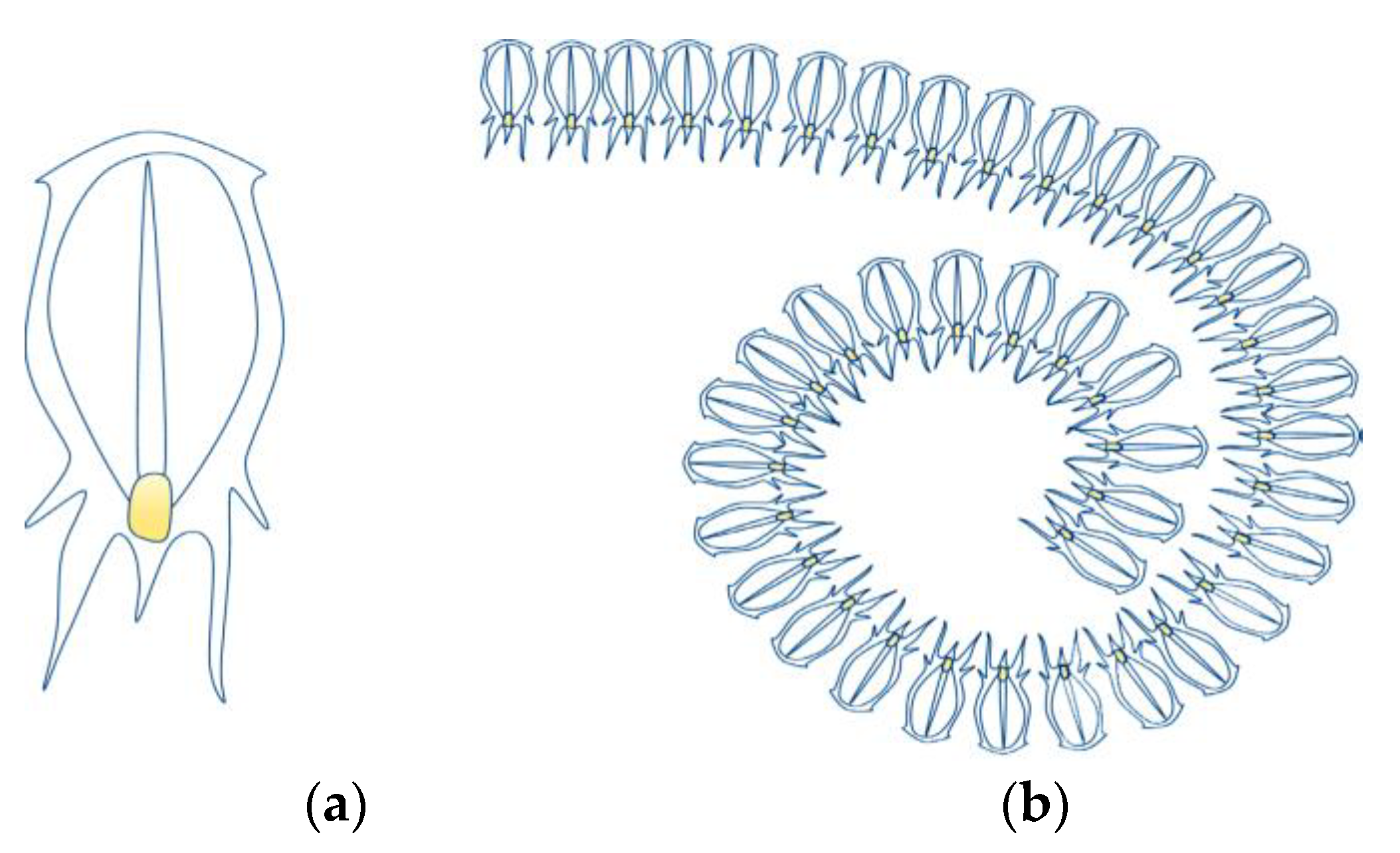
3. Salp Swarm Algorithm (SSA)

The SSA is a type of Salp family, and it is similar to a jellyfish’s body. The SSA inhabits oceans, and they derive their movement from water power to look for food, which adjust as swarms, and are known as salp chains.

The SSA typifies the solutions of the given problems by the position number of the salps, which are represented by (salp chain) in the dimension of (n × dim), where n is the search agent and dim is the proposed variable. The salp chain is categorized into two groups; the first one is the leader (in the front of the chain) and the second is the follower (all other salps in the swarm), as shown in Figure 2.

The optimal solution (the preferable salp) is considered as the swarm’s main target (food), which is followed up by the follower’s group. When the leader updates its position according to the best food, it explores the search space carefully to obtain the best solution, and the follower follows the leader.

The leader of the chain updates its place concerning a food source, which is formulated as:

$${\mathrm{A}}_{\mathrm{j}}{}^1=\{\begin{array}{c}{\mathrm{H}}_{\mathrm{j}}+{\mathrm{c}}_1\left(\left({\mathrm{U}}_{\mathrm{j}}-{\mathrm{L}}_{\mathrm{j}}\right){\mathrm{c}}_2+{\mathrm{L}}_{\mathrm{j}}\right){\mathrm{c}}_3\ge 0\\ {\mathrm{H}}_{\mathrm{j}}-{\mathrm{c}}_1\left(\left({\mathrm{U}}_{\mathrm{j}}-{\mathrm{L}}_{\mathrm{j}}\right){\mathrm{c}}_2+{\mathrm{L}}_{\mathrm{j}}\right){\mathrm{c}}_3<0\end{array}$$

(16)

${\mathrm{A}}_{\mathrm{j}}{}^1$is the leader position, ${\mathrm{H}}_{\mathrm{j}}$ is the position of the food source.

${\mathrm{L}}_{\mathrm{j}}{\mathrm{and}\mathrm{U}}_{\mathrm{j}}$represent the lower and upper boundaries, respectively. ${\mathrm{c}}_2{\mathrm{and}\mathrm{c}}_3$ are random numbers, where

$${\mathrm{c}}_1=2{\mathrm{e}}^{-{\left(\frac{4\mathrm{x}}{\mathrm{X}}\right)}^2}$$

(17)

$\mathrm{x}$ is the current iteration and $X$ is the maximum number of iterations. By Newton’s law of motion, the follower salps update their position:

$${\mathrm{A}}_{\mathrm{j}}{}^{\mathrm{i}}=\frac{1}{2}\left({\mathrm{aw}}^2+{\mathrm{v}}_{\mathrm{o}}\mathrm{wi}\right)\ge 2$$

(18)

where ${\mathrm{A}}_{\mathrm{j}}{}^{\mathrm{i}}$ is the follower salp position, $v_o$ is the initial speed, and $w$ is the number of the iteration.

Then, Equation (18) can be reorganized as:

$${\mathrm{A}}_{\mathrm{j}}{}^{\mathrm{i}}=\frac{1}{2}\left({\mathrm{A}}_{\mathrm{j}}{}^{\mathrm{i}}+{\mathrm{A}}_{\mathrm{j}}{}^{\mathrm{i}-1}\right)$$

(19)

The application of SSA for the optimal placement of DGs units can be summarized in the following steps:

• Step 1: specify the input variables of the SSA, which include the search agent, the number of iterations, and the lower and upper variable.
• Step 2: start the population of the SSA randomly, using (20).

$$\mathrm{A}\left(\mathrm{n},\mathrm{m}\right)=\mathrm{rand}\left(\mathrm{n},1\right)\ast \left(\mathrm{U}-\mathrm{L}\right)+\mathrm{L}$$

(20)

• Step 3: run the forward–backward load flow code and determine the fitness function.
• Step 4: calculate the best position according to the optimal fitness function.
• Step 5: update the position of the leader salp according to (16).
• Step 6: update the position of the follower salp according to (19).
• Step 7: verify the limits of the header and follower of the salp chain.
• Step 8: run the forward–backward load flow code in order to determine the fitness function for the positions which updated, then calculate the optimal position.
• Step 9: repeat the previous steps from step 5 to step 8 until the current iteration equals a maximum number of iterations.
• Step 10: finally, find an optimal position represented by the food source and the associated fitness function.

4. Optimal Sizes

From Figure 1, the total active power losses ($P_{Loss}$) in the RDS are calculated as:

$${\mathsf{\alpha }}_{\mathrm{ST}}=\frac{{\mathrm{R}}_{\mathrm{ST}}}{{\mathrm{V}}_{\mathrm{S}}{\mathrm{V}}_{\mathrm{T}}}\cos \left({\mathsf{\alpha }}_{\mathrm{S}}-{\mathsf{\alpha }}_{\mathrm{T}}\right)$$

(21)

$${\mathsf{\beta }}_{\mathrm{ST}}=\frac{{\mathrm{R}}_{\mathrm{ST}}}{{\mathrm{V}}_{\mathrm{S}}{\mathrm{V}}_{\mathrm{T}}}\sin \left({\mathsf{\alpha }}_{\mathrm{S}}-{\mathsf{\alpha }}_{\mathrm{T}}\right)$$

(22)

${\mathrm{V}}_{\mathrm{S}}{\mathrm{and}\mathrm{V}}_{\mathrm{T}}$ are the voltage magnitude at bus$\mathrm{S}\mathrm{and}\mathrm{T},$ respectively

${\mathrm{Z}}_{\mathrm{ST}}={\mathrm{R}}_{\mathrm{ST}}+{\mathrm{jX}}_{\mathrm{ST}}$, where ${\mathrm{Z}}_{\mathrm{ST}}$bus impedance matrix.

We assume that x is the number of the DG which supplies only active power (Type I) and their places are ${\mathrm{M}}_1,{\mathrm{M}}_2,\dots ..{\mathrm{M}}_{\mathrm{x}}$, while ${\mathrm{P}}_{{\left(\mathrm{DG}\right)}_{M_1}},{\mathrm{P}}_{{\left(\mathrm{DG}\right)}_{{\mathrm{M}}_2}}\dots \dots ..{\mathrm{P}}_{{\left(\mathrm{DG}\right)}_{{\mathrm{M}}_{\mathrm{x}}}}$ are the sizes of the DGs, respectively.

Therefore, the active power from Type I can be:

$[{\mathrm{P}}_{{\mathrm{M}}_1}={\mathrm{P}}_{{\left(\mathrm{DG}\right)}_{{\mathrm{M}}_1}}-{\mathrm{P}}_{{(\mathrm{Load})}_{{\mathrm{M}}_1}}\left],\dots \dots .,\right[{\mathrm{P}}_{{\mathrm{M}}_{\mathrm{x}}}={\mathrm{P}}_{{\left(\mathrm{DG}\right)}_{{\mathrm{M}}_{\mathrm{x}}}}-{\mathrm{P}}_{{(\mathrm{Load})}_{{\mathrm{M}}_{\mathrm{x}}}}]$. Furthermore, the number of the DGs supplying reactive power (Type II) is y, and their places are ${\mathrm{N}}_1,{\mathrm{N}}_2,\dots ..{\mathrm{N}}_{\mathrm{y}}$, while ${\mathrm{Q}}_{{\left(\mathrm{DG}\right)}_{{\mathrm{N}}_1}},{\mathrm{Q}}_{{\left(\mathrm{DG}\right)}_{{\mathrm{N}}_2}}\dots \dots ..{\mathrm{Q}}_{{\left(\mathrm{DG}\right)}_{{\mathrm{N}}_{\mathrm{y}}}}$ are the sizes of the DGs, respectively.

The reactive power from Type II can be written as: $[{\mathrm{Q}}_{{\mathrm{N}}_1}={\mathrm{Q}}_{{\left(\mathrm{DG}\right)}_{{\mathrm{N}}_1}}-{\mathrm{Q}}_{{(\mathrm{Load})}_{{\mathrm{N}}_1}}\left],\dots \dots ,\right[{\mathrm{Q}}_{{\mathrm{N}}_{\mathrm{y}}}={\mathrm{Q}}_{{\left(\mathrm{DG}\right)}_{{\mathrm{N}}_{\mathrm{y}}}}-{\mathrm{Q}}_{{(\mathrm{Load})}_{{\mathrm{N}}_{\mathrm{y}}}}].$

The minimum power losses can be obtained if the first derivative of the power losses with respect to the power supplied from the DGs becomes zero; therefore, it can be formed as:

$$\frac{\partial {\mathrm{P}}_{\mathrm{Loss}}}{\partial {\mathrm{P}}_{{\mathrm{M}}_1}}=2{\mathsf{\alpha }}_{{\mathrm{M}}_1{\mathrm{M}}_1}{\mathrm{P}}_{{\mathrm{M}}_1}+2{\displaystyle \sum }_{\begin{array}{c}\mathrm{T}=1\\ \mathrm{T}\ne {\mathrm{M}}_1\end{array}}^{\mathrm{No}}\left({\mathsf{\alpha }}_{{\mathrm{M}}_1\mathrm{T}}{\mathrm{P}}_{\mathrm{T}}-{\mathsf{\beta }}_{{\mathrm{M}}_1\mathrm{T}}{\mathrm{Q}}_{\mathrm{T}}\right)$$

(23)

or

$$\begin{gathered} {\mathsf{\alpha }}_{{\mathrm{M}}_1{\mathrm{M}}_1}{\mathrm{P}}_{{\mathrm{M}}_1}+{\mathsf{\alpha }}_{{\mathrm{M}}_1{\mathrm{M}}_2}{\mathrm{P}}_{{\mathrm{M}}_2}+\dots +{\mathsf{\alpha }}_{{\mathrm{M}}_1{\mathrm{M}}_{\mathrm{x}}}{\mathrm{P}}_{{\mathrm{M}}_{\mathrm{x}}}-{\mathsf{\beta }}_{{\mathrm{M}}_1{\mathrm{N}}_1}{\mathrm{Q}}_{{\mathrm{N}}_1}-{\mathsf{\beta }}_{{\mathrm{M}}_1{\mathrm{N}}_2}{\mathrm{Q}}_{{\mathrm{N}}_2}-\dots \\ -{\mathsf{\beta }}_{{\mathrm{M}}_1{\mathrm{N}}_{\mathrm{y}}}{\mathrm{Q}}_{{\mathrm{N}}_{\mathrm{y}}}=-{\displaystyle \sum }_{\begin{array}{c}\mathrm{T}=1\\ \mathrm{T}\ne {\mathrm{M}}_1,{\mathrm{M}}_2,\dots , {\mathrm{M}}_{\mathrm{x}}\\ \mathrm{T}\ne {\mathrm{N}}_1,{\mathrm{N}}_2,\dots ..,{\mathrm{N}}_{\mathrm{y}}\end{array}}^{\mathrm{No}}\left({\mathsf{\alpha }}_{{\mathrm{M}}_1\mathrm{T}}{\mathrm{P}}_{\mathrm{T}}-{\mathsf{\beta }}_{{\mathrm{M}}_1\mathrm{T}}{\mathrm{Q}}_{\mathrm{T}}\right) \end{gathered}$$

(24)

The derivative of the active power loss according to active power injection $P_{M_x}$ can be formulated as:

$$\frac{\partial {\mathrm{P}}_{\mathrm{Loss}}}{\partial {\mathrm{P}}_{{\mathrm{M}}_{\mathrm{x}}}}=2{\mathsf{\alpha }}_{{\mathrm{M}}_{\mathrm{x}}{\mathrm{M}}_{\mathrm{x}}}{\mathrm{P}}_{{\mathrm{M}}_{\mathrm{x}}}+2{\displaystyle \sum }_{\begin{array}{c}\mathrm{T}=1\\ \mathrm{T}\ne {\mathrm{M}}_{\mathrm{x}}\end{array}}^{\mathrm{No}}\left({\mathsf{\alpha }}_{{\mathrm{M}}_{\mathrm{x}}\mathrm{T}}{\mathrm{P}}_{\mathrm{T}}-{\mathsf{\beta }}_{{\mathrm{M}}_{\mathrm{x}}\mathrm{T}}{\mathrm{Q}}_{\mathrm{T}}\right)$$

(25)

or

$$\begin{gathered} {\mathsf{\alpha }}_{{\mathrm{M}}_{\mathrm{x}}{\mathrm{M}}_1}{\mathrm{P}}_{{\mathrm{M}}_1}+{\mathsf{\alpha }}_{{\mathrm{M}}_{\mathrm{x}}{\mathrm{M}}_2}{\mathrm{P}}_{{\mathrm{M}}_2}+\dots +{\mathsf{\alpha }}_{{\mathrm{M}}_{\mathrm{x}}{\mathrm{M}}_{\mathrm{x}}}{\mathrm{P}}_{{\mathrm{M}}_{\mathrm{x}}}-{\mathsf{\beta }}_{{\mathrm{M}}_{\mathrm{x}}{\mathrm{N}}_1}{\mathrm{Q}}_{{\mathrm{N}}_1}-{\mathsf{\beta }}_{{\mathrm{M}}_{\mathrm{x}}{\mathrm{N}}_2}{\mathrm{Q}}_{{\mathrm{N}}_2}-\dots \\ -{\mathsf{\beta }}_{{\mathrm{M}}_{\mathrm{x}}{\mathrm{N}}_{\mathrm{y}}}{\mathrm{Q}}_{{\mathrm{N}}_{\mathrm{y}}}=-{\displaystyle \sum }_{\begin{array}{c}\mathrm{T}=1\\ \mathrm{T}\ne {\mathrm{M}}_1,{\mathrm{M}}_2,\dots , {\mathrm{M}}_{\mathrm{x}}\\ \mathrm{T}\ne {\mathrm{N}}_1,{\mathrm{N}}_2,\dots ..,{\mathrm{N}}_{\mathrm{y}}\end{array}}^{\mathrm{NO}}\left({\mathsf{\alpha }}_{{\mathrm{M}}_{\mathrm{x}}\mathrm{T}}{\mathrm{P}}_{\mathrm{T}}-{\mathsf{\beta }}_{{\mathrm{M}}_{\mathrm{x}}\mathrm{T}}{\mathrm{Q}}_{\mathrm{T}}\right) \end{gathered}$$

(26)

Furthermore, the derivative of the active power losses regarding to the reactive power injection $Q_{N_1}$ can be formulated as:

$$\frac{\partial {\mathrm{P}}_{\mathrm{Loss}}}{\partial {\mathrm{Q}}_{{\mathrm{N}}_1}}=2{\mathsf{\alpha }}_{{\mathrm{N}}_1{\mathrm{N}}_1}{\mathrm{Q}}_{{\mathrm{N}}_1}+2{\displaystyle \sum }_{\begin{array}{c}\mathrm{T}=1\\ \mathrm{T}\ne {\mathrm{N}}_1\end{array}}^{\mathrm{No}}\left({\mathsf{\alpha }}_{{\mathrm{N}}_1\mathrm{T}}{\mathrm{P}}_{\mathrm{T}}-{\mathsf{\beta }}_{{\mathrm{N}}_1\mathrm{T}}{\mathrm{Q}}_{\mathrm{T}}\right)$$

(27)

or

$$\begin{gathered} {\mathsf{\beta }}_{{\mathrm{N}}_1{\mathrm{M}}_1}{\mathrm{P}}_{{\mathrm{M}}_1}+{\mathsf{\beta }}_{{\mathrm{N}}_1{\mathrm{M}}_2}{\mathrm{P}}_{{\mathrm{M}}_2}+\dots +{\mathsf{\beta }}_{{\mathrm{N}}_1{\mathrm{M}}_{\mathrm{x}}}{\mathrm{P}}_{{\mathrm{M}}_{\mathrm{x}}}-{\mathsf{\alpha }}_{{\mathrm{N}}_1{\mathrm{N}}_1}{\mathrm{Q}}_{{\mathrm{N}}_1}-{\mathsf{\alpha }}_{{\mathrm{N}}_1{\mathrm{N}}_2}{\mathrm{Q}}_{{\mathrm{N}}_2}-\dots \\ -{\mathsf{\alpha }}_{{\mathrm{N}}_1{\mathrm{N}}_{\mathrm{my}}}{\mathrm{Q}}_{{\mathrm{N}}_{\mathrm{y}}}=-{\displaystyle \sum }_{\begin{array}{c}\mathrm{T}=1\\ \mathrm{T}\ne {\mathrm{M}}_1,{\mathrm{M}}_2,\dots , {\mathrm{M}}_{\mathrm{x}}\\ \mathrm{T}\ne {\mathrm{N}}_1,{\mathrm{N}}_2,\dots ..,{\mathrm{N}}_{\mathrm{y}}\end{array}}^{\mathrm{No}}\left({\mathsf{\alpha }}_{{\mathrm{N}}_1\mathrm{T}}{\mathrm{Q}}_{\mathrm{T}}+{\mathsf{\beta }}_{{\mathrm{N}}_1\mathrm{T}}{\mathrm{P}}_{\mathrm{T}}\right) \end{gathered}$$

(28)

Similarly, the derivative for$Q_{N_y}$is

$$\frac{\partial {\mathrm{P}}_{\mathrm{loss}}}{\partial {\mathrm{Q}}_{{\mathrm{N}}_{\mathrm{y}}}}=2{\mathsf{\alpha }}_{{\mathrm{N}}_{\mathrm{y}}{\mathrm{N}}_{\mathrm{y}}}{\mathrm{Q}}_{{\mathrm{N}}_{\mathrm{y}}}+2{\displaystyle \sum }_{\begin{array}{c}\mathrm{T}=1\\ \mathrm{T}\ne {\mathrm{N}}_{\mathrm{y}}\end{array}}^{\mathrm{No}}\left({\mathsf{\alpha }}_{{\mathrm{N}}_{\mathrm{y}}\mathrm{T}}{\mathrm{P}}_{\mathrm{T}}-{\mathsf{\beta }}_{{\mathrm{N}}_{\mathrm{y}}\mathrm{T}}{\mathrm{Q}}_{\mathrm{T}}\right)$$

(29)

$$\begin{gathered} {\mathsf{\beta }}_{{\mathrm{N}}_{\mathrm{y}}{\mathrm{M}}_1}{\mathrm{P}}_{{\mathrm{M}}_1}+{\mathsf{\beta }}_{{\mathrm{N}}_{\mathrm{y}}{\mathrm{M}}_2}{\mathrm{P}}_{{\mathrm{M}}_2}+\dots +{\mathsf{\beta }}_{{\mathrm{N}}_{\mathrm{y}}{\mathrm{M}}_{\mathrm{x}}}{\mathrm{P}}_{{\mathrm{M}}_{\mathrm{x}}}-{\mathsf{\alpha }}_{{\mathrm{N}}_{\mathrm{y}}{\mathrm{N}}_1}{\mathrm{Q}}_{{\mathrm{N}}_1}-{\mathsf{\alpha }}_{{\mathrm{N}}_{\mathrm{y}}{\mathrm{N}}_2}{\mathrm{Q}}_{{\mathrm{N}}_2}-\dots \\ -{\mathsf{\alpha }}_{{\mathrm{N}}_{\mathrm{y}}{\mathrm{N}}_{\mathrm{y}}}{\mathrm{Q}}_{{\mathrm{N}}_{\mathrm{y}}}=-{\displaystyle \sum }_{\begin{array}{c}\mathrm{T}=1\\ \mathrm{T}\ne {\mathrm{M}}_1,{\mathrm{M}}_2,\dots , {\mathrm{M}}_{\mathrm{x}}\\ \mathrm{T}\ne {\mathrm{N}}_1,{\mathrm{N}}_2,\dots ..,{\mathrm{N}}_{\mathrm{y}}\end{array}}^{\mathrm{No}}\left({\mathsf{\alpha }}_{{\mathrm{N}}_{\mathrm{y}}\mathrm{T}}{\mathrm{Q}}_{\mathrm{T}}+{\mathsf{\beta }}_{{\mathrm{N}}_{\mathrm{y}}\mathrm{T}}{\mathrm{P}}_{\mathrm{T}}\right) \end{gathered}$$

(30)

After reorganizing the above equations, they can be rewritten as illustrate below:

(31)

where

$${\mathrm{H}}_{{\mathrm{M}}_{\mathrm{i}}}={\displaystyle \sum }_{\begin{array}{c}\mathrm{T}=1\\ \mathrm{T}\ne {\mathrm{M}}_1,{\mathrm{M}}_2,\dots , {\mathrm{M}}_{\mathrm{x}}\\ \mathrm{T}\ne {\mathrm{N}}_1,{\mathrm{N}}_2,\dots ..,{\mathrm{N}}_{\mathrm{y}}\end{array}}^{\mathrm{No}}\left({\mathsf{\alpha }}_{{\mathrm{M}}_1\mathrm{T}}{\mathrm{P}}_{\mathrm{T}}-{\mathsf{\beta }}_{{\mathrm{M}}_1\mathrm{T}}{\mathrm{Q}}_{\mathrm{T}}\right),\mathrm{i}=1,2,3\dots \dots \dots \dots \mathrm{x}$$

(32)

$${\mathrm{I}}_{{\mathrm{Y}}_{\mathrm{i}}}={\displaystyle \sum }_{\begin{array}{c}\mathrm{T}=1\\ \mathrm{T}\ne {\mathrm{M}}_1,{\mathrm{M}}_2,\dots , {\mathrm{M}}_{\mathrm{x}}\\ \mathrm{T}\ne {\mathrm{N}}_1,{\mathrm{N}}_2,\dots ..,{\mathrm{N}}_{\mathrm{y}}\end{array}}^{\mathrm{No}}\left({\mathsf{\alpha }}_{{\mathrm{N}}_1\mathrm{T}}{\mathrm{Q}}_{\mathrm{T}}+{\mathsf{\beta }}_{{\mathrm{N}}_1\mathrm{T}}{\mathrm{P}}_{\mathrm{T}}\right),\mathrm{i}=1,2,3\dots \dots \dots \dots \mathrm{y}$$

(33)

If we assume the matrix in (31) is equal:

(34)

(35)

Then, after reorganization, it becomes:

$$\left[\begin{array}{cc}{\left[{\mathrm{A}}_{11}\right]}_{\mathrm{x}\times \mathrm{x}}& {\left[{\mathrm{A}}_{12}\right]}_{\begin{array}{c}x\times y\end{array}}\\ {\left[{\mathrm{A}}_{21}\right]}_{\mathrm{y}\times \mathrm{x}}& {\left[{\mathrm{A}}_{22}\right]}_{\mathrm{y}\times \mathrm{y}}\end{array}\right]\left[\begin{array}{c}{\left[{\mathrm{P}}_{{\mathrm{M}}_{\mathrm{i}}}\right]}_{\mathrm{x}\times 1}\\ {\left[{\mathrm{Q}}_{{\mathrm{N}}_{\mathrm{i}}}\right]}_{\mathrm{y}\times 1}\end{array}\right]=\left[\begin{array}{c}{\left[{\mathrm{H}}_{{\mathrm{M}}_{\mathrm{i}}}\right]}_{\mathrm{x}\times 1}\\ {\left[{\mathrm{I}}_{{\mathrm{N}}_{\mathrm{i}}}\right]}_{\mathrm{y}\times 1}\end{array}\right]$$

(36)

Next

$$\left[\begin{array}{c}{\left[{\mathrm{P}}_{{\mathrm{M}}_{\mathrm{i}}}\right]}_{\mathrm{x}\times 1}\\ {\left[{\mathrm{Q}}_{{\mathrm{N}}_{\mathrm{i}}}\right]}_{\mathrm{y}\times 1}\end{array}\right]=\mathrm{inverse}\left[\begin{array}{cc}{\left[{\mathrm{A}}_{11}\right]}_{\mathrm{x}\times \mathrm{x}}& {\left[{\mathrm{A}}_{12}\right]}_{\mathrm{x}\times \mathrm{y}}\\ {\left[{\mathrm{A}}_{21}\right]}_{\mathrm{y}\times \mathrm{x}}& {\left[{\mathrm{A}}_{22}\right]}_{\mathrm{y}\times \mathrm{y}}\end{array}\right]\left[\begin{array}{c}{\left[{\mathrm{H}}_{{\mathrm{M}}_{\mathrm{i}}}\right]}_{\mathrm{x}\times 1}\\ {\left[{\mathrm{I}}_{{\mathrm{N}}_{\mathrm{i}}}\right]}_{\mathrm{y}\times 1}\end{array}\right]$$

(37)

Then

$$\mathrm{Inverse}\left[\begin{array}{cc}{\left[{\mathrm{A}}_{11}\right]}_{\mathrm{x}\times \mathrm{x}}& {\left[{\mathrm{A}}_{12}\right]}_{\mathrm{y}\times \mathrm{x}}\\ {\left[{\mathrm{A}}_{21}\right]}_{\mathrm{y}\times \mathrm{x}}& {\left[{\mathrm{A}}_{22}\right]}_{\mathrm{y}\times \mathrm{y}}\end{array}\right]=\left[\begin{array}{cc}\left[{\mathrm{A}\text{’}}_{11}\right]& \left[{\mathrm{A}\text{’}}_{12}\right]\\ \left[{\mathrm{A}\text{’}}_{21}\right]& \left[{\mathrm{A}\text{’}}_{22}\right]\end{array}\right]$$

(38)

$${\left[{\mathrm{P}}_{{\mathrm{M}}_{\mathrm{i}}}\right]}_{\mathrm{x}\times 1}={\left[{\mathrm{A}\text{’}}_{11}\right]}_{\mathrm{x}\times \mathrm{x}}{\left[{\mathrm{H}}_{{\mathrm{M}}_{\mathrm{i}}}\right]}_{\mathrm{x}\times 1}+{\left[{\mathrm{A}\text{’}}_{12}\right]}_{\mathrm{x}\times \mathrm{y}}{\left[{\mathrm{I}}_{\mathrm{N}}\right]}_{\mathrm{y}\times 1}$$

(39)

$${\left[{\mathrm{Q}}_{{\mathrm{N}}_{\mathrm{i}}}\right]}_{\mathrm{y}\times 1}={\left[{\mathrm{A}\text{’}}_{21}\right]}_{\mathrm{y}\times \mathrm{x}}{\left[{\mathrm{H}}_{{\mathrm{M}}_{\mathrm{i}}}\right]}_{\mathrm{x}\times 1}+{\left[{\mathrm{A}\text{’}}_{22}\right]}_{\mathrm{y}\times \mathrm{y}}{\left[{\mathrm{I}}_{{\mathrm{N}}_{\mathrm{i}}}\right]}_{\mathrm{y}\times 1}$$

(40)

Finally, after the installed DG at bus $S$, the active power obtained can be calculated from the following equation:

$${\left[{\mathrm{P}}_{{\left(\mathrm{DG}\right)}_{{\mathrm{M}}_{\mathrm{i}}}}\right]}_{\mathrm{x}\times 1}={\left[{\mathrm{P}}_{{\mathrm{M}}_{\mathrm{i}}}\right]}_{\mathrm{x}\times 1}+{\mathrm{P}}_{{(\mathrm{Load})}_{\mathrm{i}}}$$

(41)

${\mathrm{P}}_{{(\mathrm{Load})}_{\mathrm{i}}}$: active power demand at bus$M_i$.

The reactive power installed from type II can be determined from the following equation:

$${\left[{\mathrm{Q}}_{{\left(\mathrm{DG}\right)}_{{\mathrm{N}}_{\mathrm{i}}}}\right]}_{\mathrm{y}\times 1}={\left[{\mathrm{Q}}_{{\mathrm{N}}_{\mathrm{i}}}\right]}_{\mathrm{y}\times 1}+{\mathrm{Q}}_{{(\mathrm{Load})}_{\mathrm{i}}}$$

(42)

${\mathrm{Q}}_{{(\mathrm{Load})}_{\mathrm{i}}}$: reactive power demand at bus $N_i$.

Note that:

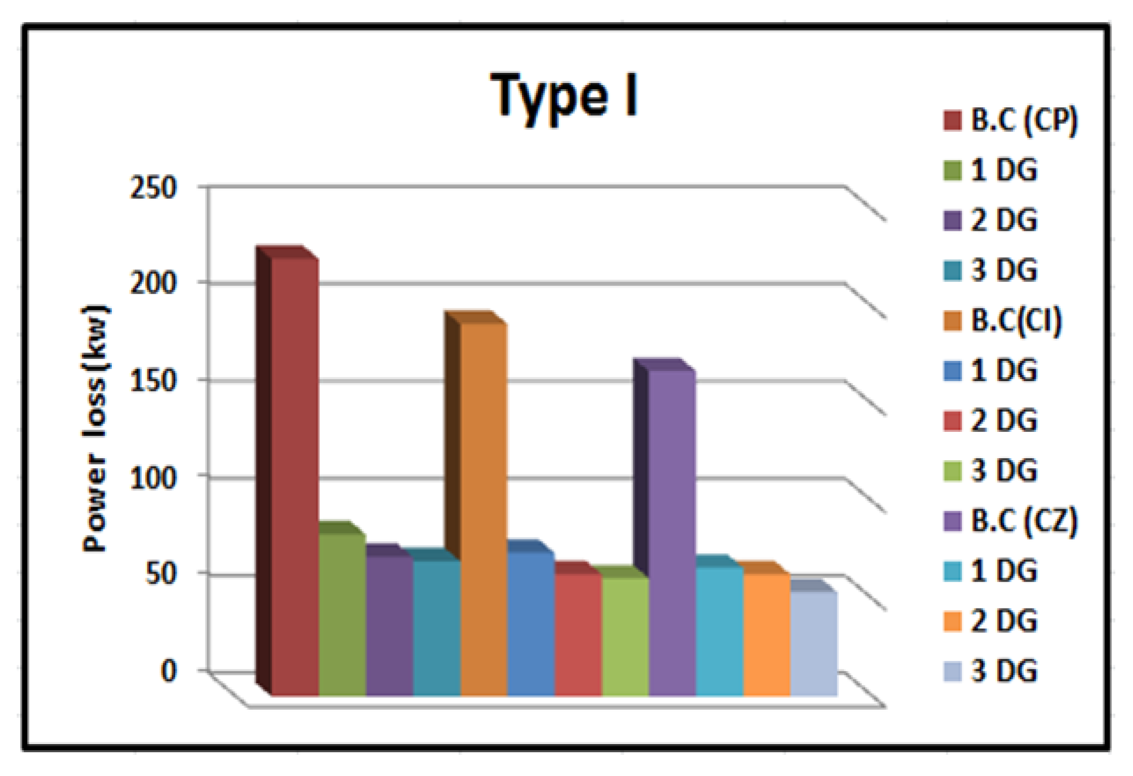
• For type I of the DG, $M_S\ne N_T\forall T$
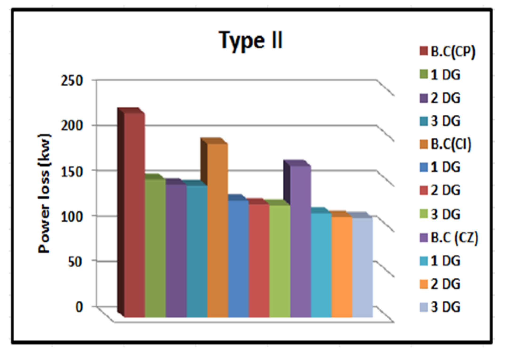
• For type II of the DG, $N_S\ne M_T\forall T$
• For type III of the DG, $M_S=N_T$

The power factor of Type III (injects active and reactive power) is calculated using (41) and (42), which can be evaluated as:

$$\mathrm{PF}=\frac{{\mathrm{P}}_{{\left(\mathrm{DG}\right)}_{\mathrm{i}}}}{\sqrt{{\mathrm{P}}_{{\left(\mathrm{DG}\right)}_{\mathrm{i}}}{}^2+{\mathrm{Q}}_{{\left(\mathrm{DG}\right)}_{\mathrm{i}}}{}^2}}$$

(43)

5. Results and Discussion

In the present work, two IEEE systems were chosen to check the effectiveness of the proposed technique. The IEEE 33-bus and IEEE 69-bus are shown in Figure 3 and Figure 4; their base voltages and apparent power are 12.66 kV and 100 MVA, respectively.

In order to obtain the optimal size and location of the DGs, the SSA is performed 100 times, and the optimal solutions are reported in tables for three load types. Furthermore, the main parameters of the SSA are specified as several search agents (=30), and the number of maximum iterations = 80.

In the present work, the simulation results of each system are divided to three cases; one DG integration, two DG integrations, and three DG integrations with three DG types and three types of loads: CP, CI, and CZ.

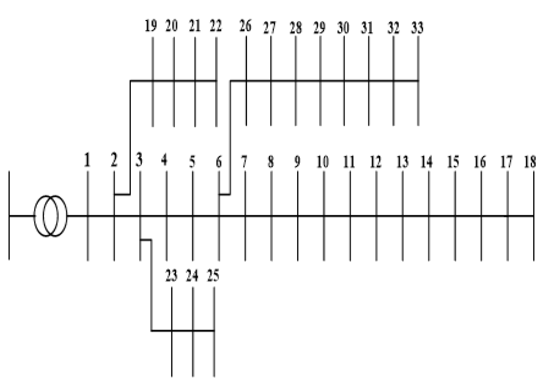
5.1. IEEE 33-Bus Test System

This system consists of 33 buses and 32 branches. The total active power of the load is 3715 kW, and the total reactive power of the load is 2300 kVAR; the total power loss at base case (B.C) is 211 kW, and the minimum voltage is 0.9040 p.u. on bus 18. The convergence characteristics of one, two, and three DGs of type I, type II, and Type III for the three loads are presented in Figure 5, Figure 6 and Figure 7, respectively. Figure 8, Figure 9, Figure 10, Figure 11, Figure 12, Figure 13, Figure 14, Figure 15 and Figure 16 describe the voltage profiles of 1DG, 2DG, and 3DG of the three DG types for the three load types. Furthermore, the power loss comparison between the three types of the load is shown in Figure 17, Figure 18 and Figure 19.

As shown in the tables, the best results (minimum power losses and maximum voltage profile) are obtained in case of three DGs type III compared with other types of DGs as provide active and reactive power to the system. Furthermore, the results obtained in case of constant impedance is better than the results in other types of loads.

5.1.1. Case1: One DG Integration

For one DG installing, the results are illustrated in

Table 1. Optimal results of one DG integration for the three loads on IEEE 33-bus RDS.

Type of Load	CP Type Load				CI Type Load				CZ Type Load
DG type	B.C	DG type			B.C	DG type			B.C	DG type
		Type-I	Type-II	Type-III		Type-I	Type-II	Type-III		Type-I	Type-II	Type-III
Location		6	30	30		6	30	6		6	30	6
Size		2.490	1.23	3.028		2.352	1.144	2.844		2.166	1.080	2.648
Total capacity		2.490	1.23	3.028		2.352	1.144	2.844		2.166	1.080	2.648
Power loss (P.L)	210.997	111.17	151.41	67.95	184.3557	96.6	133.6	63.7	159.78	86.2	115.4	52.7
V. min (p.u.)	0.9038	0.9410	0.9162	0.9570	0.9113	0.9460	0.9226	0.9664	0.9173	0.9491	0.9280	0.9632
Min voltage bus	(18)	(18)	(18)	(18)	(18)	(18)	(18)	(18)	(18)	(18)	(18)	(18)
P.L Reduction%		47.31	28.24	67.795		47.07	26.79	65.10		46.53	28.41	67.31

with the CP, CI, and CZ load types. It is shown from Table 1 that DG type III gives the best simulation results among the other DG types.

For the CP load: Bus 6 is the optimal bus for DG type I with size 2.490 MW, bus 30 for DG type II, and DG type III with sizes 1.23 MVAR and 3.028 MVA, respectively; the active power loss decreased from 210.997 kW to111.17 kW for DG type I, 151.41 kW for DG type II, and 67.95 kW for DG type III.

For the CI load: Bus 6 is specified as the optimal bus for DG type I with size 2.352 MW, bus 30 for DG type II with size 1.144 MVAR, and bus 6 for DG type III with size 2.844 MVA. The active power loss decreased from 184.355 kW to 96.6 kW at DG type I, 133.6 kW for DG type II, and 63.7 kW for DG type III.

For the CZ load: Bus 6 is specified as the optimal bus for DG type I with size 2.166 MW, bus 30 for DG type II with size 1.080 MVAR, and bus 6 for DG type III with size 2.648MVA. The power loss decreased from 159.78 kW to 86.2 kW for DG type I, 115.4 kW for DG type II, and 52.7 kW for DG type III.

5.1.2. Case2: Two DGs Integration

For two DG installation,

Table 2. Optimal results of two DG integration for three types of loads on the IEEE 33-bus RDS.

Type of Load	CP Type Load				CI Type Load				CZ Type Load
DG type	B.C	DG type			B.C	DG type			B.C	DG type
		Type-I	Type-II	Type-III		Type-I	Type-II	Type-III		Type-I	Type-II	Type-III
Location		13 30	12 30	13 30		12 30	12 30	12 30		12 30	12 30	12 30
Size		0.832 1.110	0.430 1.044	0.920 1.529		0.869 1.014	0.400 0.971	0.962 1.396		0.806 0.929	0.391 0.911	0.9 1.29
Total capacity		1.942	1.47	2.449		1.883	1.372	2.358		1.734	1.303	2.19
Power loss (P.L)	210.997	87.2876	141.935	28.56	184.356	77	125.6	27	159.78	69.9	108	24.6
V. min (p.u.)	0.9038	0.9667	0.9290	0.9801	0.9113	0.9659	0.9344	0.9836	0.9173	0.9675	0.9394	0.9814
Min voltage bus	(18)	(33)	(18)	(25)	(18)	(18)	(18)	(25)	(18)	(18)	(18)	(25)
P.L reduction%		58.63	32.73	86.46		57.81	31.2	85.21		56.64	33.00	84.74
PF				0.91 0.72		-		0.91 0.72				0.90 0.71

illustrates the results of optimal allocation of three types of DGs for three load types.

For the CP load: the power loss reduced from 210.997 kW to 87.2876 kW for DG type I, 141.935 kW for DG type II, and 28.56 kW for DG type III.

For the CI load: Bus 12 and 30 were chosen as the best locations for three DG types of DG, and the power loss reduced from 184.3557 kW to 77 kW, 125.6 kW, and 27 kW for DG type I, DG type II, and DG type III, respectively.

For the CZ load: the power loss reduced from 159.78kW to 69.9kW, 108kW, and 24.6kW for DG type I, DG type II, and DG type III, respectively, when the DGs were installed at bus 12 and 30 for the three types of DGs.

5.1.3. Case 3: Three DGs Integration

For the installation of three DGs, the optimal allocation of the three types of DGs are 13, 24, and 30 for the CP, CI, and CZ load types, as obtained in

Table 3. Optimal results of the three DGs’ integration for three types of loads on an IEEE 33 bus.

Type of Load	CP Type Load				CI Type Load				CZ Type Load
DG type	B.C	DG type			B.C	DG type			B.C	DG type
		Type-I	Type-II	Type-III		Type-I	Type-II	Type-III		Type-I	Type-II	Type-III
Location		13 24 30	13 24 30	13 24 30		13 24 30	13 24 30	13 24 30		13 24 30	13 24 30	13 24 30
Size		0.79 1.07 1.012	0.359 0.52 1.016	0.869 1.189 1.425		0.725 0.958 1.046	0.334 0.490 0.944	0.802 1.175 1.337		0.672 1.015 0.871	0.324 0.490 0.884	0.750 1.128 1.234
Total capacity		2.87	1.890	3.483		2.730	1.769	3.297		2.558	1.699	3.112
Power loss (P.L)	210.997	72.89	138.37	11.77	184.3557	63.6	122.4	11.3	159.78	57	104.9	9.5
V. min (p.u.)	0.9038	0.9670	0.9303	0.9905	0.9113	0.9695	0.9356	0.9918	0.9173	0.9713	0.9405	0.9925
Min voltage bus	(18)	(33)	(18)	(8)	(18)	(33)	(18)	(8)	(18)	(18)	(18)	(8)
P.L reduction%	-	65.45	34.42	94.42		65.15	32.93	93.81		64.64	34.92	94.11
	-
PF				0.91 0.90 0.71		-		0.91 0.91 0.71				0.90 0.90 0.70

; the power loss reduction is at its maximum in the case of the type III DGs in all three types of load among the other types, as they inject active and reactive power.

Furthermore, the power losses for the three previous tables with the number of iterations are shown in Figure 5, Figure 6 and Figure 7.

For the CP load: the power loss reached 72.89 kW in DG type I, 138.37 kW in DG type II, and 11.77 kW in DG type III from B.C 210.997 kW.

In order to further emphasize the strength of the proposed method,

Table 4. Optimal results of the three DGs for type III compared with other techniques for CP loads on an IEEE 33 bus.

Case	Technique	Location Size (MVA)				Total Capacity (MVA)	Power Loss	P.f	V min (p.u.)	Loss Reduction %
3DG	Proposed	Bus	13	24	30	3.483	11.77	0.91 0.90 0.71	0.9905 (8)	94.42
		Size	0.869	1.189	1.425
	GA [26]	Bus	14	24	30	3.407	11.91	0.90 0.89 0.72	NA	94.35
		Size	0.8153	1.102	1.49
	IA [27]	Bus	6	30	14	2.964	22.29	0.82 0.82 0.82	0.99217 (8)	89.45
		Size	1.098	1.098	0.768
	PABC [28]	Bus	12	25	30	2.889	15.91	0.85 0.85 0.85	NA	92.46
		Size	1.014	0.960	1.363

illustrates a comparison between the proposed method results and other techniques for the CP load case; the maximum benefit can be achieved at this case as the number of the DGs which inject active and reactive power are increased, so that the minimum power losses are achieved and the voltages of all of the buses are improved when the three DGs are placed at the optimal locations, with optimal power factors of 0.91, 0.90, and 0.71, respectively.

The proposed method achieves a power loss reduction of 94.42%, which is better than other techniques, e.g., 89.45% and 89.43 in Improved Analytical (IA) [27] and Particle Artificial Bee Colony algorithm (PABC) [28].

For the CI load: the B.C power losses are 184.3557 kW; the power losses obtained in the case of inserting three DGs of DG type I is 63.6 kW, DG type II is 122.4kW, and DG type III is 11.3kW.

For the CZ load: the power loss reached 57 kW in DG type I, 104.9 kW in DG type II, and 9.5 kW in DG type III from B.C 159.78 kW.

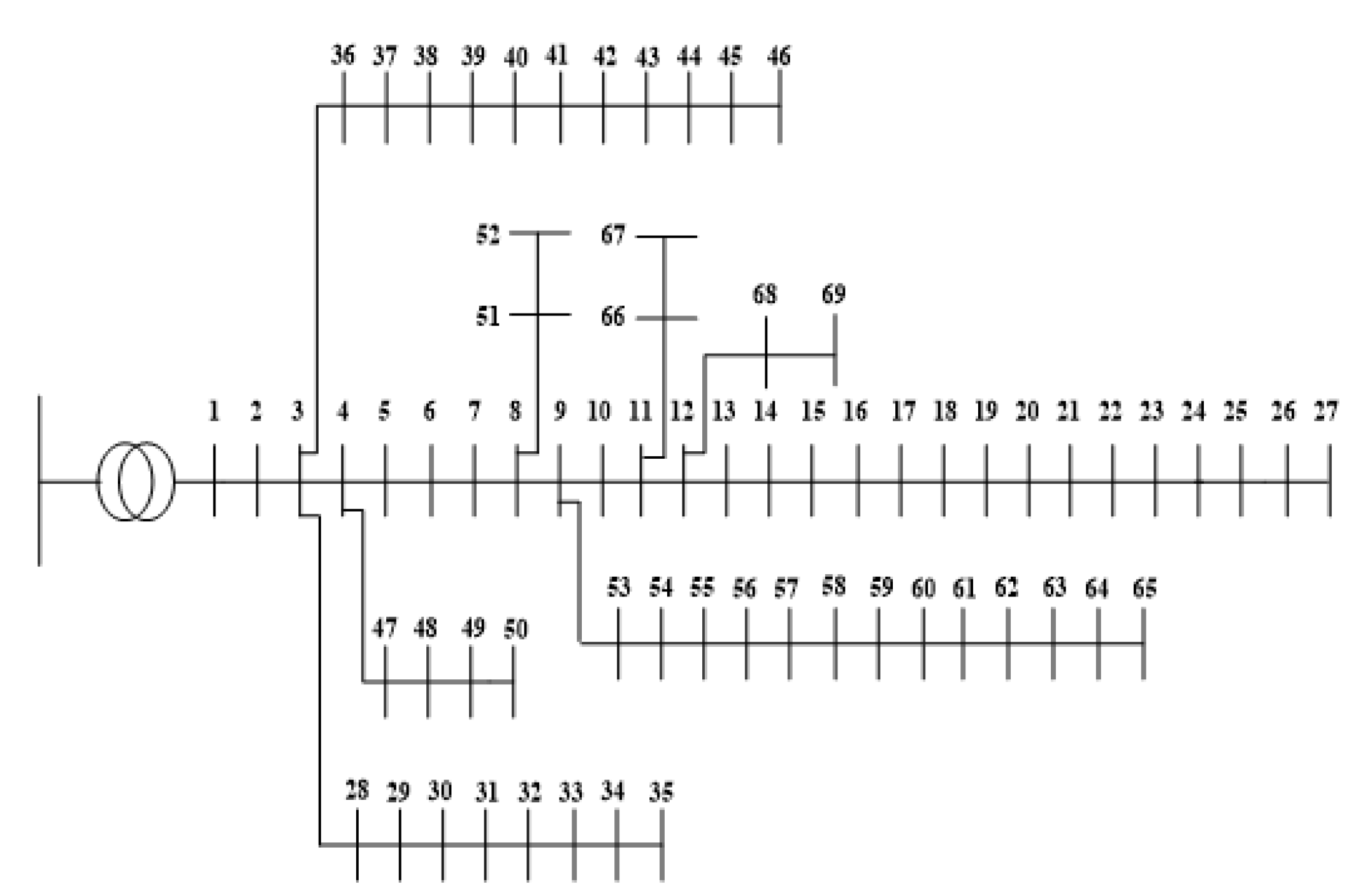
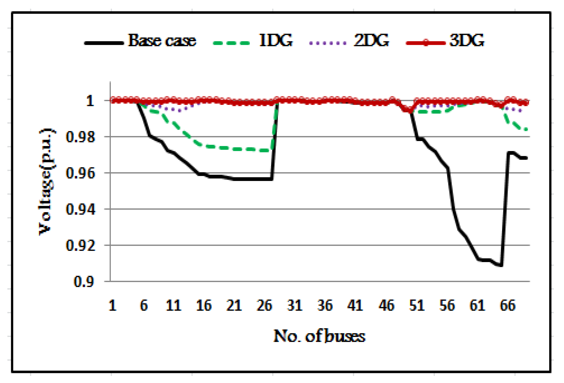
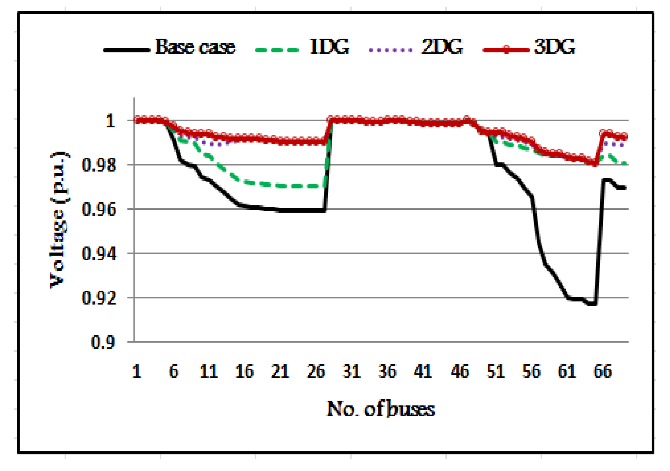
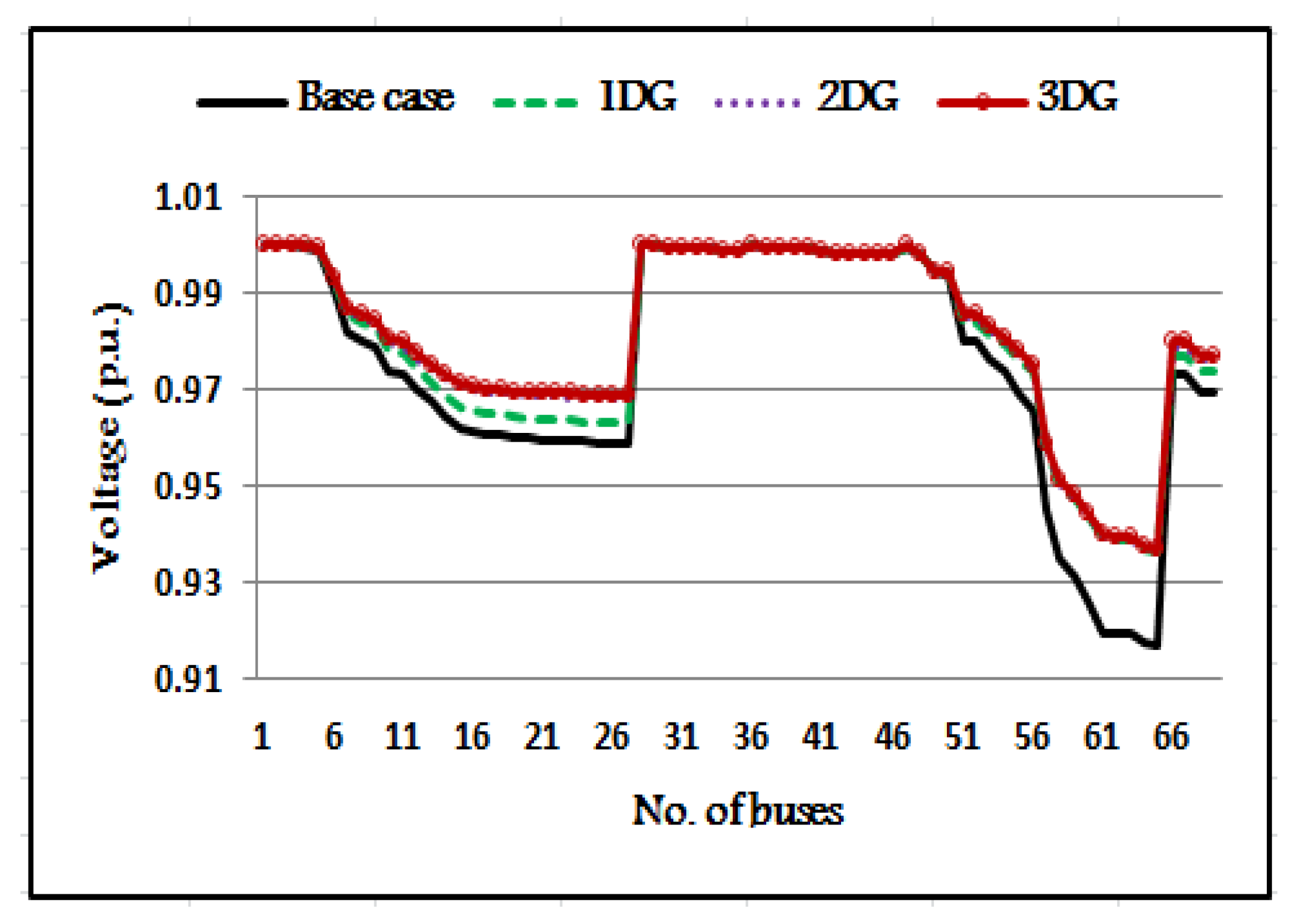
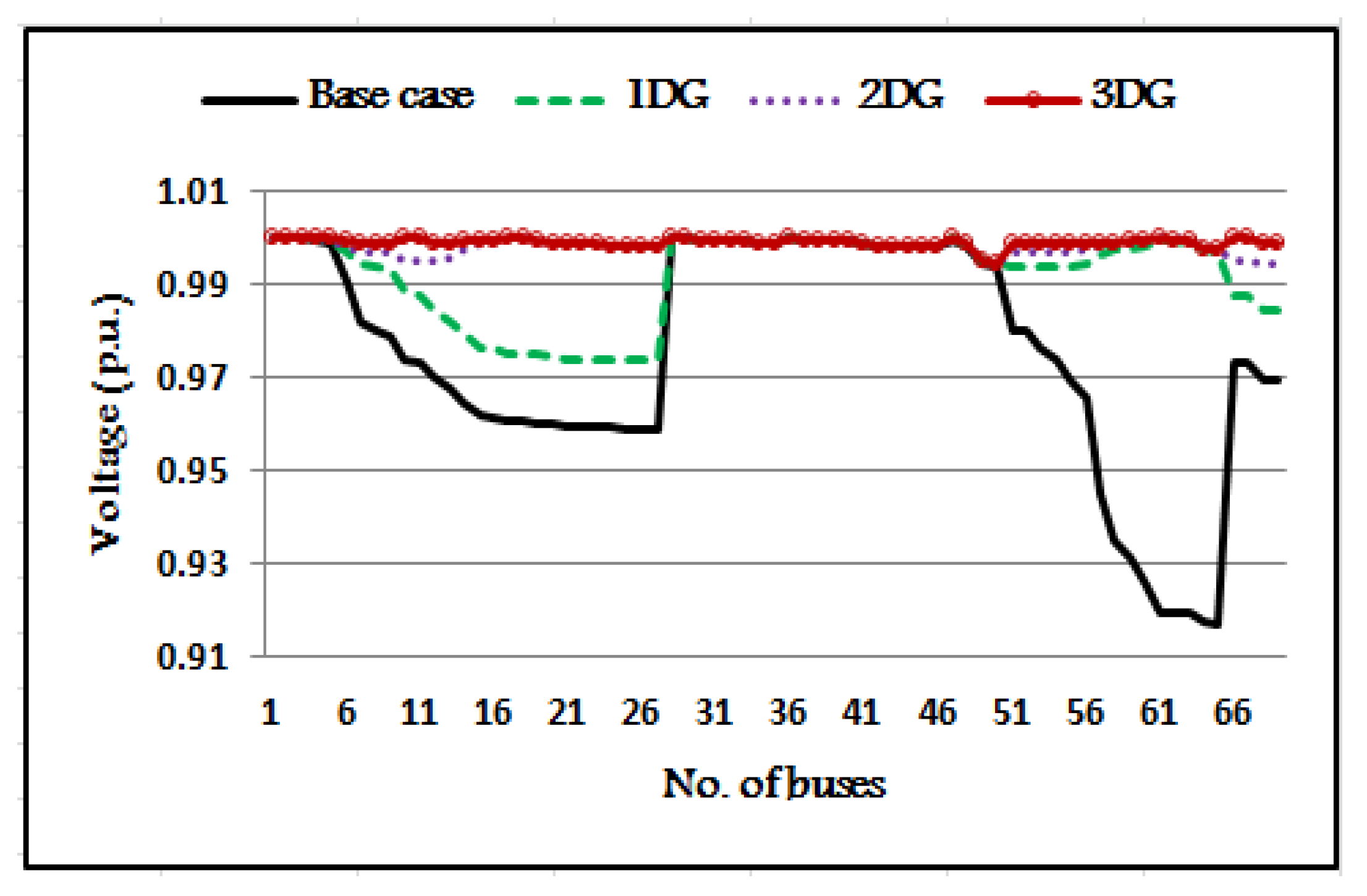
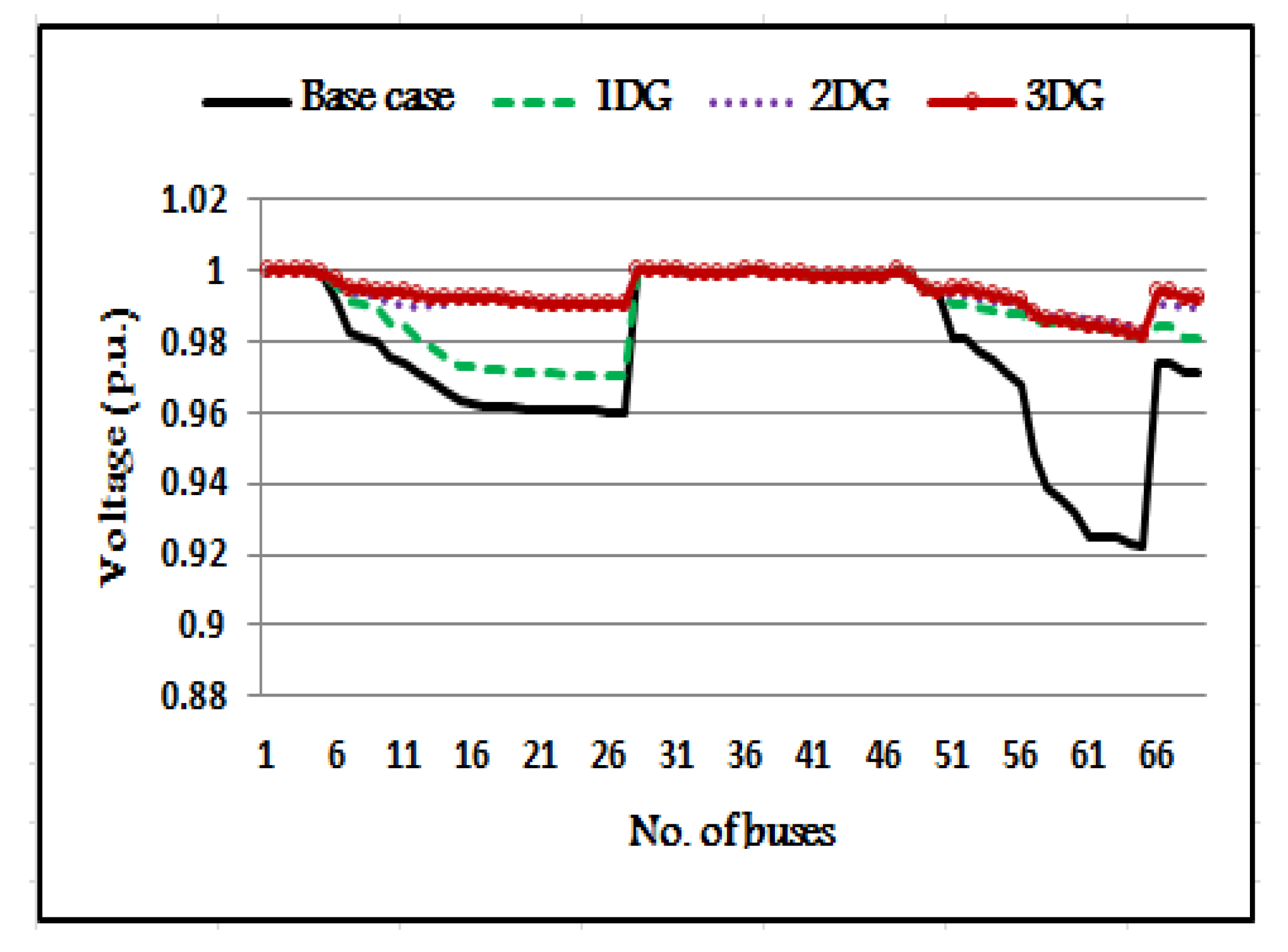
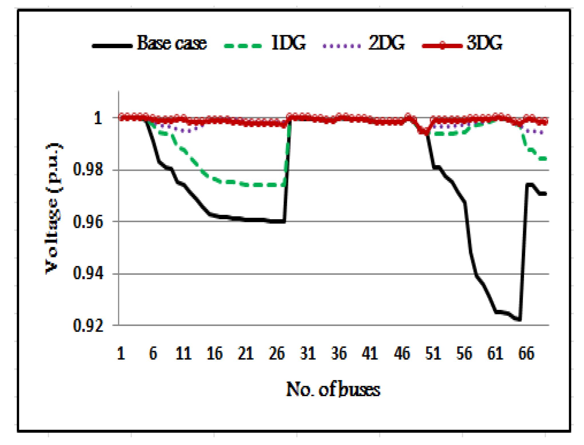
5.2. IEEE 69-Bus Test System

This system consists of 69 buses and 68 branches, as shown in Figure 6; the total active and reactive power of the load are 3801.49 kW and 2694.6 KVAR, respectively; the losses at base case (B.C) are 224.997 kW, and the minimum voltage is 0.9091 p.u. at bus 65. The convergence characteristics of one, two, and three DGs of DG type I, DG type II, and DG type III for the three loads are presented in Figure 20, Figure 21 and Figure 22, respectively. Figure 23, Figure 24, Figure 25, Figure 26, Figure 27, Figure 28, Figure 29, Figure 30 and Figure 31 describe the voltage profiles of 1DG, 2DG, and 3DG of the three DG types for the three load types. Furthermore, the power loss comparisons between the three types of load are shown in Figure 32, Figure 33 and Figure 34.

Similar to the IEEE 33 bus, the minimum power losses in the case of three DGs for type III were constant impedance (CZ) and then constant current (CI), followed by constant power (CP), although most locations of the DGs were the same for the three type of loads. The power factor was improved for three cases.

5.2.1. Case1: One DG Integration

For one DG installation, the simulation results are illustrated in

Table 5. Optimal results of one DG integration for three types of loads on an IEEE 69 bus RDS.

Type of Load	CP Type Load				CI Type Load				CZ Type Load
Case	B.C	DG type			B.C	DG type			B.C	DG type
DG type		Type-I	Type-II	Type-III		Type-I	Type-II	Type-III		Type-I	Type-II	Type-III
Location		61	61	61		61	61	61		61	61	61
Size		18.1	1.291	2.22		1.655	1.202	2.052		1.594	1.122	1.924
Total capacity		18.1	1.291	2.22		1.655	1.202	2.052		1.594	1.122	1.924
Power loss (PL)	224.997	83.37	152.09	23.15	191.5	73.87	129	22	167.2	66.2	115	21
V. min (p.u.)	0.9091	0.9679	0.9302	0.9734	0.9167	0.9690	0.9361	0.9740	0.9226	0.9700	0.9402	0.9748
Min voltage bus	(65)	(27)	(65)	(27)	(65)	(27)	(65)	(27)	(65)	(27)	(65)	(27)
P.L reduction%		62.95	32.40	89.71		61.43	32.63	88.5		60.40	31.22	87.44
PF				0.81				0.81				0.81

.

For the CP load: Bus 61 is the optimal bus for three types of DG; the power loss decreased from 224.997 kW to 83.37 kW for DG type I, 152.09 kW for DG type II, and 23.15 kW for DG type III.

For the CI load: Bus 61 is the optimal bus for the three types of DGs; the power loss decreased from 191.5 kW to 73.87 kW for DG type I, 129 kW for DG type II, and 22 kW for DG type III.

For the CZ load: the power losses reduced from 167.2kW at B.C to 66.2kW for DG type I, to 115 kW for DG type II, and to 21 kW for DG type III when the DG was installed at bus 6.

5.2.2. Case2: Two DGs Integration

For two DG installation, the simulation results are illustrated in

Table 6. Optimal results of two DG integration for three types of loads on an IEEE 69 bus RDS.

	CP Type Load				CI Type Load				CZ Type Load
Type of load	B.C	DG type			B.C	DG type			B.C	DG type
DG type		Type-I	Type-II	Type-III		Type-I	Type-II	Type-III		Type-I	Type-II	Type-III
Location		61 17	61 17	61 17		61 17	61 17	61 17		61 17	61 17	61 17
Size		1.724 0.518 2.24	1.236 0.35 1.586	2.127 0.626 2.752		1.575 0.497 2.072	1.147 0.336 1.483	1.979 0.606 2.585		1.583 0.507 2.090	1.069 0.326 1.395	1.834 0.559 2.393
Total capacity
Power loss (PL)	224.997	71.804	146.51	7.1857	191.5	62.87	124.84	6.87	167.2	62.82	110.9	6.8
V. min (p.u.)	0.9091	0.9769	0.9305	0.9946	0.9167	0.9783	0.9364	0.9946	0.9226	0.9801	0.9405	0.9940
Min voltage bus	(65)	(65)	(65)	(69)	(65)	(65)	(65)	(69)	(65)	(65)	(65)	(69)
PL reduction%		68.09	34.88	96.8		67.17	30.80	96.41		66.69	33.67	95.93
PF				0.81 0.83				0.81 0.83				0.81 0.81

.

For the CP load: the proposed hybrid method chose buses 61and 17 as the optimal locations for the three types of load, and the power loss reached 71.804 kW for DG type I. 146.51 kW for DG type II, and 7.1857 kW for DG type III from the base case 224.997 kW.

For the CI load: in the constant current load, the power loss reduced from 191.5 kW to 62.87 kW, 124.84 kW, and 6.87 kW for DG type I, DG type II, and DG type III, respectively.

For the CZ load: the power loss was reduced from 167.2kW at B.C to 62.82 kW for DG type I, to 110.9kW for DG type II, and to 6.8 kW for DG type III when the DGs were installed at bus 61 and 17, which are the best locations for the three types of the DG.

5.2.3. Case 3: Three DG Integration

For three DGs installation, the simulation results are illustrated in

Table 7. Optimal results of the three DG integration for the three loads on an IEEE 69-bus RDS.

Type of Load	CP Type Load				CI Type Load				CZ Type Load
DG type	B.C	DG type			B.C	DG type			B.C	DG type
		Type-I	Type-II	Type-III		Type-I	Type-II	Type-III		Type-I	Type-II	Type-III
Location		11 18 61	11 21 61	11 18 61		11 18 61	11 18 61	11 18 61		11 18 61	11 18 61	11 18 61
Size		0.499 0.377 1.668	0.368 0.231 1.196	0.616 0.452 2.050		0.491 0.359 1.520	0.336 0.241 1.109	0.604 0.438 1.884		0.493 0.358 1.427	0.336 0.231 1.031	0.602 0.425 1.758
Total capacity		2.545	1.795	3.119		2.370	1.686	2.926		2.278	1.597	2.785
Power loss (P.L)	224.997	69.5456	145.21	4.25	191.5	60.70	123.67	4	167.2	53.6	109.7	3.9
V. min (p.u.)	0.9091	0.9770	0.9307	0.9972	0.9167	0.9785	0.9367	0.9974	0.9226	0.9802	0.9408	0.9975
Min voltage bus	(65)	(65)	(65)	(65)	(65)	(65)	(65)	(65)	(65)	(65)	(65)	(50)
P.L reduction%	-	69.09	35.46	98.11		68.3	35.42	97.91		67.94	34.39	97.67
	-
PF				0.82 0.81 0.81		-		0.82 0.84 0.81				0.82 0.84 0.81

.

For CP load: the proposed hybrid method specified buses 61, 18, and 11 as the optimal locations for type I and type III, while the buses 11, 21, and 61 are the best for DG type II, and the power losses reached 69.5456 kW for DG type I, 145.21 kW for DG type II, and 4.25 kW for DG type III from B.C 224.997 kW. It was observed that DG type III obtained less power loss compared with the others.

In a 69-bus system, the proposed method achieved the best results compared with the other techniques in the case of three DG integration for type III, as shown in

Table 8. Optimal results of three DGs for type III compared with the other techniques for CP loads on an IEEE 69 bus.

Case	Technique	(Location) Size (MVA)				Total Capacity (MVA)	Power Loss	P.f	V min	Loss Reduction%
1 DG	Proposed	Bus	61			2.22	23.15	0.81	0.9734	89.71
		Size	2.22
	GA [29]	Bus	61			2.16	38.45	NA	NA	82.91
		Size	2.16
3 DG	Proposed	Bus	11	18	61	3.119	4.25	0.82 0.81 0.81	0.9972 (65)	98.11
		Size	0.616	0.452	2.050
	Hybrid [30]	Bus	18	61	66	3.07	4.30	0.77 0.83 0.82	NA	98.1
		Size	0.48	2.06	0.53
	CPLS [31]	Bus	21	61	64	3.356	7.1	0.81 0.81 0.81	0.9934 (69)	96.84
		Size	0.723	2.20	0.438
	EA [32]	Bus	11	18	61	3.239	4.48	0.82 0.83 0.82	NA	NA
		Size	0.668	0.458	2.113
	EA-OPF [32]	Bus	11	18	61	3.134	4.27	0.81 0.83 0.81	NA	NA
		Size	0.611	0.456	2.067

, when the three DGs are placed at 11, 21, and 61; with an optimal power factor of 0.82, 0.81, and 0.81, respectively, the power loss reduction for the proposed method is 98.11%, which is better than 98.10 in the Hybrid PSO-Analytical [26] and 96.84 in the combined power loss sensitivity (CPLS).

For CI load: the power loss was reduced from 191.5 kW to 60.70 kW, 123.67 kW, and 4 kW for DG type I, DG type II, and DG type III, respectively.

For CZ load: the best voltage profile and minimum power loss were obtained in this type of load when the three types of DGs were placed at 11, 18, and 61 for the three types of loads.

6. Conclusions

This paper presented an efficient hybrid analytical and metaheuristic technique to find the optimal locations and sizes of different and multiple types of DGs in order to minimize active power losses and improve the overall voltage profile. The hybrid technique was applied to three types of static loads in order o check the robustness of the proposed method. A metaheuristic SSA technique was proposed in order to ascertain the optimal allocation of the DG units in the three types of loads—CP, CI, and CZ—while the analytical technique determined the proper sizes. The proposed algorithm was tested on 33-bus and 69-bus systems, and the results illustrated in the tables and figures proved that the power loss reduction reaches the maximum value in the case of the incorporation of three DGs of type III for the three types of loads.

References

1. Reddy, P.D.P.; Reddy, V.C.V.; Manohar, T.G. Whale optimization algorithm for optimal sizing of renewable resources for loss reduction in distribution systems. Renew. Wind Water Sol. 2017, 4, 1–13. [Google Scholar] [CrossRef] [Green Version]
2. Kazerani, M.; Tehrani, K. Grid of Hybrid AC/DC Microgrids: A New Paradigm for Smart City of Tomorrow. In Proceedings of the 2020 IEEE 15th International Conference of System of Systems Engineering (SoSE), Budapest, Hungary, 2–4 June 2020; pp. 175–180. [Google Scholar]
3. Kemikem, D.; Boudour, M.; Benabid, R.; Tehrani, K. Quantitative and Qualitative Reliability Assessment of Reparable Electrical Power Supply Systems using Fault Tree Method and Importance Factors. In Proceedings of the 2018 13th Annual Conference on System of Systems Engineering (SoSE), Paris, France, 19–22 June 2018; pp. 452–458. [Google Scholar]
4. Singh, R.K.; Goswami, S.K. Optimum allocation of distributed generations based on nodal pricing for profit, loss reduction and voltage improvement including voltage rise issue. Electr. Power Energy Syst. 2010, 32, 637–644. [Google Scholar] [CrossRef]
5. Caponetto, R.; Fortuna, L.; Fazzino, S.; Xibilia, M.G. Chaotic sequences to improve the performance evolutionary algorithms. IEEE Trans. Evol. Comput. 2003, 7, 289–304. [Google Scholar] [CrossRef]
6. Ali, E.S.; Abd Elazim, S.M.; Abdelaziz, A.Y. Optimal allocation and sizing of renewable distributed generation using ant lion optimization algorithm. Electr. Eng. 2018, 100, 99–109. [Google Scholar] [CrossRef]
7. El-Zonkoly, A. Optimal placement of multi-distributed generation units including different load models using particle swarm optimisation. IET Gener. Transm. Distrib. 2011, 5, 760–771. [Google Scholar] [CrossRef]
8. Moradi, M.; Abedini, M. A combination of genetic algorithm and particle swarm optimization for optimal DG location and sizing in distribution systems. Int. J. Electr. Power Energy Syst. 2012, 34, 66–74. [Google Scholar] [CrossRef]
9. Abu-Mouti, F.S.; El-Hawary, M.E. Optimal distributed generation allocation and sizing in distribution systems via artificial bee colony algorithm. IEEE Trans. Power Deliv. 2011, 26, 2090–2101. [Google Scholar] [CrossRef]
10. García, J.A.M.; Mena, A.J.G. Optimal distributed generation location and size using a modified teaching–learning based optimization algorithm. Int. J. Electr. Power Energy Syst. 2013, 50, 65–75. [Google Scholar] [CrossRef]
11. Nekooei, K.; Farsangi, M.M.; Nezamabadi-Pour, H.; Lee, K.Y. An improved multi-objective harmony search for optimal placement of DGs in distribution systems. IEEE Trans. Smart Grid 2013, 4, 557–567. [Google Scholar] [CrossRef]
12. Kaur, S.; Kumbhar, G.; Sharma, J. A MINLP technique for optimal placement of multiple DG units in distribution systems. Int. J. Electr. Power Energy Syst. 2014, 63, 609–617. [Google Scholar] [CrossRef]
13. Hosseini, S.A.; Madahi, S.S.K.; Razavi, F.; Karami, M.; Ghadimi, A.A. Optimal sizing and siting distributed generation resources using a multiobjective algorithm. Turk. J. Electr. Eng. Comput. Sci. 2013, 21, 825–850. [Google Scholar]
14. Sultana, U.; Khairuddin, A.B.; Aman, M.; Mokhtar, A.; Zareen, N. A review of optimum DG placement based on minimization of power losses and voltage stability enhancement of distribution system. Renew. Sustain. Energy Rev. 2016, 63, 363–378. [Google Scholar] [CrossRef]
15. Singh, A.; Parida, S. Novel sensitivity factors for DG placement based on loss reduction and voltage improvement. Int. J. Electr. Power Energy Syst. 2016, 74, 453–456. [Google Scholar] [CrossRef]
16. Prakash, D.B.; Lakshminaraya, C. Optimal siting of capacitors in radial distribution network using whale optimization algorithm. Alex. Eng. J. 2016. [Google Scholar] [CrossRef] [Green Version]
17. Khodabakhshian, A.; Andishgar, M.H. Simultaneous Placement and Sizing of DGs and Shunt Capacitors in Distribution Systems by Using IMDE algorithm. Electr. Power Energy Syst. 2016, 82, 599–607. [Google Scholar] [CrossRef]
18. Haque, M.H. Load flow-solution of distribution systems with voltage dependent load models. Electr. Power Syst. Res. 1996, 36, 151–156. [Google Scholar] [CrossRef]
19. Roy, N.K.; Hossain, M.J.; Pota, H.R. Voltage profile improvement for distributed wind generation using D-STATCOM. In Proceedings of the IEEE PES General Meeting, Detroit, MI, USA, 24–28 July 2011. [Google Scholar]
20. Dahal, S.; Mithulananthan, N.; Saha, T. Investigation of small signal stability of a renewable energy based electricity distribution system. In Proceedings of the IEEE PES General Meeting, Minneapolis, MN, USA, 25–29 July 2010. [Google Scholar]
21. Mirjalili, S.; Gandomi, A.H.; Mirjalili, S.Z.; Saremi, S.; Faris, H.; Mirjalili, S.M. Salp Swarm Algorithm: A bio-inspired optimizer for engineering design problems. Adv. Eng. Softw. 2017, 114, 163–191. [Google Scholar] [CrossRef]
22. Sayed, G.I.; Khoriba, G.; Haggag, M.H. A novel chaotic salp swarm algorithm for global optimization and feature selection. Appl. Intell. 2018, 48, 3462–3481. [Google Scholar] [CrossRef]
23. El-Fergany, A.A. Extracting optimal parameters of PEM fuel cells using salp swarm optimizer. Renew. Energy 2018, 119, 641–648. [Google Scholar] [CrossRef]
24. Qais, M.H.; Hasanien, H.M.; Alghuwainem, S. Enhanced salp swarm algorithm: Application to variable speed wind generators. Eng. Appl. Artif. Intell. 2019, 80, 82–96. [Google Scholar] [CrossRef]
25. El-Fergany, A.A.; Hasanien, H.M. Salp swarm optimizer to solve optimal power flow comprising voltage stability analysis. Neural Comput. Appl. 2019, 32, 5267–5283. [Google Scholar] [CrossRef]
26. Moradi, M.H.; Abedinie, M.; Tolabi, H.B. Optimal multi-distributed generation location and capacity by genetic algorithms. In Proceedings of the 2010 Conference Proceedings IPEC, Singapore, 27–29 October 2010; pp. 614–618. [Google Scholar]
27. Hung, D.Q.; Mithulananthan, N. Multiple distributed generator placement in primary distribution networks for loss reduction. IEEE Trans. Ind. Electron. 2011, 60, 1700–1708. [Google Scholar] [CrossRef]
28. Muthukumar, K.; Jayalalitha, S. Optimal placement and sizing of distributed generators and shunt capacitors for power loss minimization in radial distribution networks using hybrid heuristic search optimization technique. Int. J. Electr. Power Energy Syst. 2016, 78, 299–319. [Google Scholar] [CrossRef]
29. Shukla, T.; Singh, S.; Srinivasarao, V.; Naik, K. Optimal sizing of distributed generation placed on radial distribution systems. Electr. Power Compon. Syst. 2010, 38, 260–274. [Google Scholar] [CrossRef]
30. Kansal, S.; Kumar, V.; Tyagi, B. Hybrid approach for optimal placement of multiple DGs of multiple types in distribution networks. Int. J. Electr. Power Energy Syst. 2016, 75, 226–235. [Google Scholar] [CrossRef]
31. Kumar, A.; Babu, P.V.; Murty, V.V.S.N. Distributed generators allocation in radial distribution systems with load growth using loss sensitivity approach. J. Inst. Eng. (India) Ser. B 2017, 98, 275–287. [Google Scholar] [CrossRef]
32. Mahmoud, K.; Yorino, N.; Ahmed, A. Optimal distributed generation allocation in distribution systems for loss minimization. IEEE Trans. Power Syst. 2015, 31, 960–969. [Google Scholar] [CrossRef]
Figure 1. Two bus radial distribution network.
Sustainability 13 04447 g001
Figure 2. (a) Individual salp; (b) swarm of salps (salps chain) [19].
Sustainability 13 04447 g002
Figure 3. Single line diagram of the 33-bus system.
Sustainability 13 04447 g003
Figure 4. Single line diagram of the 69-bus system.
Sustainability 13 04447 g004
Figure 5. Pl and Iter of DG type I for the three loads.
Sustainability 13 04447 g005
Figure 6. Pl and Iter of DG type II for the three loads.
Sustainability 13 04447 g006
Figure 7. Pl and Iter of DG type III for the three loads.
Sustainability 13 04447 g007
Figure 8. Voltage profile of DG type I for the CP load.
Sustainability 13 04447 g008
Figure 9. Voltage profile of DG type II for the CP load.
Sustainability 13 04447 g009
Figure 10. Voltage profile of DG type III for the CP load.
Sustainability 13 04447 g010
Figure 11. Voltage profile of DG type I for the CI load.
Sustainability 13 04447 g011
Figure 12. Voltage profile of DG type II for the CI load.
Sustainability 13 04447 g012
Figure 13. Voltage profile of DG type III for the CI load.
Sustainability 13 04447 g013
Figure 14. Voltage profile of DG type I for the CZ load.
Sustainability 13 04447 g014
Figure 15. Voltage profile of DG type II for the CZ load.
Sustainability 13 04447 g015
Figure 16. Voltage profile of DG type III for the CZ load.
Sustainability 13 04447 g016
Figure 17. The power loss of DG type I for the three loads.
Sustainability 13 04447 g017
Figure 18. The power loss of DG type II for the three loads.
Sustainability 13 04447 g018
Figure 19. The power loss of DG type III for the three loads.
Sustainability 13 04447 g019
Figure 20. Pl and Iter of DG type I for the three loads.
Sustainability 13 04447 g020
Figure 21. Pl and Iter of DG type II for the three loads.
Sustainability 13 04447 g021
Figure 22. Pl and Iter of DG type III for the three loads.
Sustainability 13 04447 g022
Figure 23. Voltage profile of DG type I for the CP load.
Sustainability 13 04447 g023
Figure 24. Voltage profile of DG type II for the CP load.
Sustainability 13 04447 g024
Figure 25. Voltage profile of DG type III for the CP load.
Sustainability 13 04447 g025
Figure 26. Voltage profile of DG type I for the CI load.
Sustainability 13 04447 g026
Figure 27. Voltage profile of DG type II for the CI load.
Sustainability 13 04447 g027
Figure 28. Voltage profile of DG type III for the CI load.
Sustainability 13 04447 g028
Figure 29. Voltage profile of DG type I for the CZ load.
Sustainability 13 04447 g029
Figure 30. Voltage profile of DG type II for the CZ load.
Sustainability 13 04447 g030
Figure 31. Voltage profile of DG type III for the CZ load.
Sustainability 13 04447 g031
Figure 32. The power loss of DG type I for the three loads.
Sustainability 13 04447 g032
Figure 33. The power loss of DG type II for the three loads.
Sustainability 13 04447 g033
Figure 34. The power loss of DG type III for the three loads.
Sustainability 13 04447 g034