Article

Optimized Land Use through Integrated Land Suitability and GIS Approach in West El-Minia Governorate, Upper Egypt

by
Yasser M. Zakarya
1,
Mohamed M. Metwaly
2,
Mohamed A. E. AbdelRahman
3,*,
Mohamed R. Metwalli
2 and
Georgios Koubouris
4,*
1
Faculty of Agriculture, Ain-Shams University, Cairo 11241, Egypt
2
Data Reception, Analysis and Receiving Station Affairs Division, National Authority for Remote Sensing and Space Sciences, Cairo 11769, Egypt
3
Land Use Department, Division of Environmental Studies and Land Use, National Authority for Remote Sensing and Space Sciences (NARSS), Cairo 11769, Egypt
4
ELGO DIMITRA, Institute of Olive Tree, Subtropical Crops and Viticulture, 731 36 Chania, Greece
*
Authors to whom correspondence should be addressed.
Sustainability 2021, 13(21), 12236; https://doi.org/10.3390/su132112236
Submission received: 11 August 2021 / Revised: 1 November 2021 / Accepted: 2 November 2021 / Published: 5 November 2021
(This article belongs to the Collection Sustainable Soil Management in a Changing Climate)

Abstract

:
Land evaluation is imperative for its efficient use in agriculture. Therefore, this study aimed at assessing the suitability of a region in West El-Minia for cultivating some of the major crops using the geographical information system (GIS). The results focus on allocating space for cultivating sugar beet and utilizing the free period of sugar beet in other crops. This exploitation helps to maintain the quality of the land and increase its fertility by using crop rotation with integrated agricultural management. A machine learning technique was implemented using the random forest algorithm (RF) to predict soil suitability classes for sugar beet using geomorphology, terrain attribute and remote sensing data. Fifteen major crops were evaluated using a suitability multicriteria approach in GIS environment for crop rotation decisions. Soil parameters were determined (soil depth, pH, texture, CaCO3, drainage, ECe, and slope) to characterize the land units for soil suitability. Soils of the area were found to be Entisols; Typic Torrifluvents, Typic Torripsamments and Typic Torriorthents and Aridsols; Typic Haplocacids, Calcic Haplosalids and Sodic Haplocalcids. Overall, the studied area was classified into four suitability classes: high “S1”, moderate “S2”, marginal “S3”, and not suitable “N”. The area of each suitability class changed depending on the crop tested. The highest two crops that occupied S1 class were barley with 471.5 ha (representing 6.8% of the total study area) and alfalfa with 157.4 ha (2.3%). In addition, barley, sugar beet, and sorghum occupied the highest areas in S2 class with 6415.3 ha (92.5%), 6111.3 ha (88.11%) and 6111.3 ha (88.1%), respectively. Regarding the S3 class, three different crops (sesame, green pepper, and maize) were the most highly represented by 6151.8 ha (88.7%), 6126.3 ha (88.3%), and 6116.7 ha (88.2%), respectively. In the end, potato and beans occupied the highest areas in N class with 6916.9 ha (99.7%) and 6853.5 ha (98.8%), respectively. The results revealed that the integration of GIS and soil suitability system consists of an appropriate approach for the evaluation of suitable crop rotations for optimized land use planning and to prevent soil degradation. The study recommends using crop rotation, as it contributes to soil sustainability and the control of plant pests and diseases, where the succession of agricultural crops on a scientific basis aims at maintaining the balance of nutrients and fertilizers in the soil.

1. Introduction

Egypt suffers from water deficit, which affects agricultural production, as well as the growing gap between food production and consumption for most agricultural crops in light of the continuous population increase [1]. Therefore, there is a need to set restrictions and determinants of agriculture and reconsider the current and proposed crop structures in modern reclamation places, which maximizes the net return on the water unit used to achieve the highest net return per unit of cultivated area, and of course for farmers, which contributes to raising the standard of living. The land suitability is the efficiency of the land with the specific soil properties along with topographic and climatic factors to be suitable for the effective growth of a particular type of plant on a sustainable basis [2,3]. Depending on the soil properties and topographical features, the land can be categorized into potential areas for cultivation [4]. Agricultural suitability assessment is the evaluation of the methodological performance of land when using alternative cultivation options [5,6]. The primary purpose of assessing the suitability of agricultural land is to predict the potential and limitations of land for crop production [7]. Either the rotation of large fields or within-field diversity in strip-cropping annual systems will diversify the income stream and protect against a weak market for a single commodity. Several researchers [8,9] have documented remote sensing and geographic information system capabilities to assess land suitability. GIS tools and remote sensing data suggest a suitable and influential platform to integrate spatially complex land attributes for carrying out land suitability analysis [2,3,10,11]. A combination of GIS and multicriteria evaluation techniques with a weighted overlay approach for land suitability analysis proves to be a useful methodology for further research in the concept of crop suitability for the optimized irrigation method [12]. The suitability of agricultural land for the area was not documented previously.
Geologically, the area consists of limestone, sandstone, and air sediments method [13]; the fact that most of the region consists of limestone land is suitable for growing crops that suit limestone land. An evaluation of the region’s cultivation of many crops was made, and it was concluded that beet cultivation is the best high-yield agricultural use according to soil characteristics and climatic conditions. Because the beets crop season lasts for approximately eight months, the land is free from plantations for more than four months. Therefore, to maximize the economic return from the land, several crops are proposed, including tomatoes and peanuts.
The sugar beet crop is considered one of the most economically important crops for sugar production, and its importance is due to the relaxation of sucrose, which has a high nutritional value, which is used in human food as a source of high energy. The sugar beet is considered a dual-purpose crop, as it is extracted from the sugar root, and the vegetative complex is used as food for animals. Moreover, the cultivation of beets improves the properties of the soil, especially in saline lands as well as in reclamation and limestone lands. Beet cultivation provides many job opportunities, both in the field and in sugar factories. Beet sugar contributes about 1.06 million tons, representing about 53% of the total sugar production. In general, and to increase sugar production through the cane, there are many problems and obstacles, which have increased the importance of beet sugar in reducing the size of the sugar gap in Egypt [14].
Crop rotation is a method of growing several crops in the same field and producing high yields without weakening the soil. It includes a group of different methods of production in order to find the best way to use the land. Farmers must take into account soil composition and slope, drainage, and soil erosion problems when deciding what types of crops are suitable for their land, as well as the history of land use in the production of previous crops. Various combinations of production methods, such as different cultivation techniques, crop rotation and the correct use of fertilizers and pesticides, are used to assist farmers. One of the oldest and most widespread methods of soil conservation is the use of a crop cycle. It is the alternation of crops grown in the fields from year to year, as one crop consumes the mineral salts and organic matter in the soil if it is grown in the same field year after year. However, planting different types of crops in the field according to a regular schedule provides an opportunity to replace most of the mineral salts and organic matter, and also helps reduce plant diseases and the life cycle of insects; for example, corn takes nitrogen from the soil, while other crops, such as alfalfa, excrete it. Corn was planted in the field once, so it is possible to plant alfalfa the following year. This is to replace the nitrogen consumed by the corn. It is also possible to plow the soil with nitrogen-producing crops so that these crops remain inside the soil, and when they decay, they replace most of the lost organic matter and enrich the soil. On sloping lands, weeds and deep-rooted crops are replaced with other crops in order to maintain soil cohesion and prevent erosion. In intensive agricultural systems, the use of fertilizers is gradually replacing the crop rotation as a method of producing crops that achieve the highest profits year after year while keeping the soil fertile. Nitrifying and other fertilizers have been developed that help restore lost mineral salts from the soil. When these fertilizers are added—and with the use of appropriate tillage methods and pesticides—it becomes possible to grow the same crop annually without damaging the soil. Other developments in the agricultural production system include chemical pesticides that kill insects, weeds and microorganisms.
Machine learning (ML) is a sub-field of computer science, closely related to statistics, which aims to make computers learn from data without explicit programming. ML models are capable of discovering knowledge, important relationships, and integrating different types of data easily by learning. These ML models include artificial neural networks, partial least squares regressions, support vector machines, generalized additive models, genetic programming, regression tree models, k-nearest neighbor regression, adaptive neuro-fuzzy inference system, and random forests. Because of their high accuracy, resilience, and ease of use, random forests and support vector machines are the most widely employed approaches in the digital soil mapping community in recent years [15].
Instead of employing a single classifier, numerous authors attempted to improve the efficiency of the classification process by using a set of classifiers. The “ensemble” classification methods are those that use a set of classifiers to predict class labels. The multiple classifier system (MCS) or ensemble approaches are rapidly growing and gaining a lot of attention; they were shown to be more accurate and robust than a single classifier in a variety of domains. These techniques typically function by means of firstly building an ensemble of base classifiers by applying a given base learning algorithm to various alternative permutated training sets, and then combining the outputs from each ensemble member in a suitable way to create the prediction of the ensemble classifier. The combination is often performed by voting for the most popular class [16]. Examples of these techniques include Bagging, AdaBoost, and RUSBoost. Ensemble classification using the RUSBoost technique results in improved classification performance when training data are imbalanced [17].
ML models are used in the digital soil mapping framework to link soil observations and auxiliary variables in order to investigate spatial and temporal variation in soil classes and other soil properties. These auxiliary variables can be obtained from digital elevation models (DEM), remotely sensed data (RS), and other geo-spatial data sources [15,18]. Khaledian et al. (2020) [19] examined the strengths and disadvantages of six ML algorithms, “k-nearest neighbors (KNN), multiple linear regression (MLR), Cubist, support vector regression (SVR), random forest (RF), and artificial neural networks (ANN)”, for digital soil mapping. The results demonstrated that MLR, SVR, and ANN are more prone to overfitting, whereas RF algorithm avoids the risk of overfitting, and takes less time to compute. Both ANN and RF perform well in predicting non-linear patterns, while the RF is faster, and overcomes the weakness of ANN sensitivity to small datasets.
The aim of the research is to arrive at the best models for crop composition of crops and vegetables in a manner that is compatible with the available water resources to achieve development goals in terms of maximizing economic efficiency. More specifically, the purpose of this paper is to (a) shed light on the suitability of the agricultural land of the region for sugar beet as a promising crop; (b) calculate the extent of suitability of agricultural lands; and (c) categorize each specific topic with the appropriateness of agricultural lands.

2. Materials and Methods
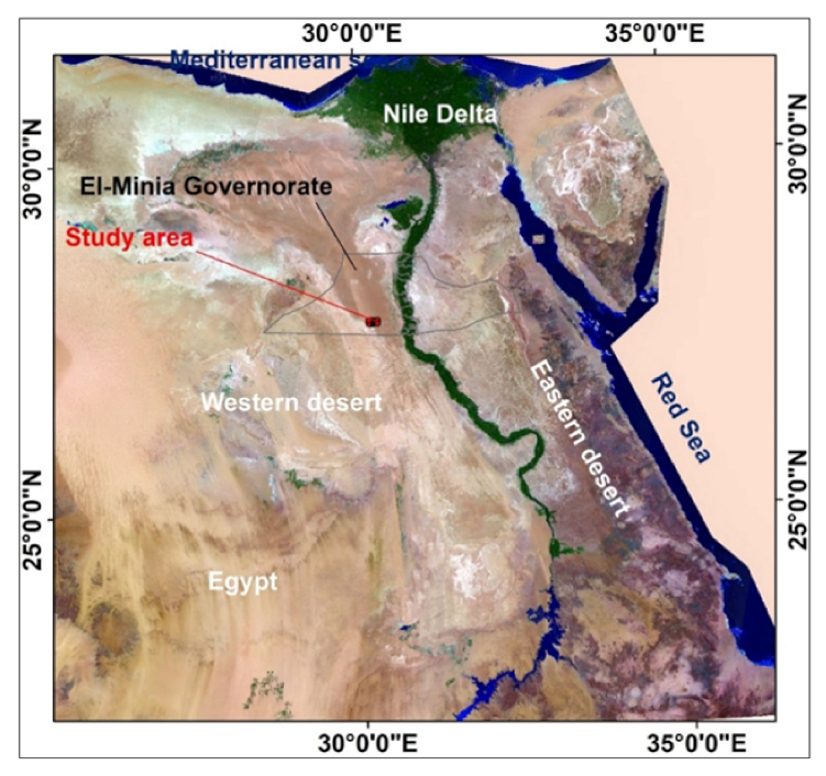
2.1. Study Area

This study was conducted on soil samples collected from (27°39′31″ N, 30°9′2″ E) and (27°16′6″ N, 30°17′56″ E), located in the newly reclaimed area of the western part of El Minia Governorate as shown in Figure 1. The profiles were dug before the planting of the study area. The area topography is undulating with 6935.63 ha. The most common land use in this area includes farming sugar beet, tomato, sesame, wheat and sunflower.

2.2. Climate Factors

The study area climate is classified as arid to semi-arid with a dry hot summer, while winter is mild or rainless. The annual average, mean minimum and mean maximum temperatures are presented in Table 1.

2.3. Experiment Design

Distances among neighboring points were 500–600 m, distributed uniformly to meet the geostatistical interpolation requirements. The soil samples depth was based on the difference of layers along with the profile depths. The interpolations were performed for the surface layers of all profiles, while the interpretation of soils was described based on the weighted average of all profile’s layers. A total of 208 soil profiles were dug and morphologically described [20]. The total soil samples (542) from horizons and layers of the soil profile were subjected to various physical and chemical analyses (CaCO3, ECe, pH, Sp and soil texture).

2.4. Land Use Types and Crop Requirements

The selection of suitable land use types for each crop was determined based on the local conditions, i.e., local food needs, crop area coverage, social acceptability and economical sustainability. Land use requirements determine the types of data that need to be collected for a land evaluation and described by the land properties. In determining the requirements of the land utilization types, the main consideration was given to the physical and chemical requirements, whereas the climatic requirements were not considered because the whole area belongs to only one agroecological zone; therefore, the climatic conditions are uniform. Based on the existing cropping systems in the surrounding area, fifteen land use types were selected as indicated in Supplementary Tables S1–S15 according to Sys, 1993 [21] and Zakarya, 2009 [22].

2.5. Interpolation Methods

Thematic maps for each of the soil parameters and slope were developed using ArcGIS 10.2 software. Thematic maps of the study area were generated, using inverse distance weighted (IDW) interpolation as recommended by [23]. IDW interpolation determines cell values, using a linearly weighted combination of a set of sample points.
The following equation was used for IDW and kriging interpolation methods as well-discussed by Yao et al. [24]:
Z X 0 = i = 1 n w i Z x i
where the Z(xi) data value of locations is used to generate the variable Z value of X0 the unsampled location; the Z(xi) value is assigned by the weight wi, n is the number of the used closest neighboring data points for estimation.
w i = 1 d i 2 i = 1 n 1 d i 2
where di is the distance between the estimated point and the observed point.
γ h = 1 2 n i = 1 n [ Z x i Z x i + h ) ] 2
where x i and x i + h are sampling locations separated by a distance h, and Z x i and Z x i + h are the observed values of variable Z at the corresponding locations.
The least squares method, which was used to estimate the linear regression, is the following equation:
y = B 0 + x + a n = i = 1 n B i X i

2.6. Land Suitability Evaluation Model Steps

In order to identify a land suitability class, the following steps could be summarized as depicted in Figure 2: (1) The features of the major physical and chemical soil properties values (soil depth, CaCO3, soil texture (sand, silt and clay), ECe, and pH) were stored in shapefile format. (2) The slope percent was estimated from DEM. (3) The shapefile was converted to raster format using the IDW interpolation method in ArcGIS 10.2. Thereafter, reclassified layers were overlaid by a raster calculator. These overlaid layers were used to assess land suitability for these crops. Based on the above-mentioned soils, the studied areas were categorized into four groups: S1 (highly suitable), S2 (moderately suitable), S3 (marginally suitable) and N (not suitable). (4) The crop requirements were established following the approach of [22,25]. The selected crops that were evaluated for this specific study included sugar beet, wheat, barley, alfalfa, sunflower, sorghum, soybean, sesame, groundnut, green pepper, onion, tomato, potato, beans and maize. In this particular land suitability analysis for selected major crops, the criteria are mainly related to topography (slope) and soil (soil depth, soil pH, soil texture and soil drainage). These are the most important requirements needed for all crops according to opinions of agronomist experts and literature review. Factor ratings are sets of values that indicate how well each factor is satisfied by particular conditions of the corresponding land suitability. (5) Finally, current suitability was calculated using the reclassify tool in ARCGIS to classify the soil properties layer into categories (S1, S2, S3, N1 and N2) according to the crop requirements adopted after [21,22,26].

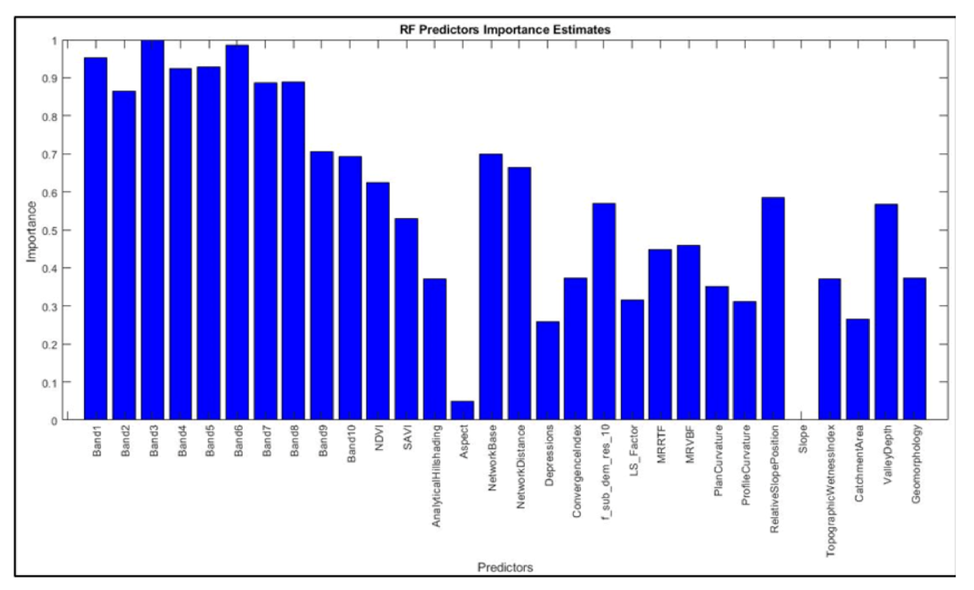
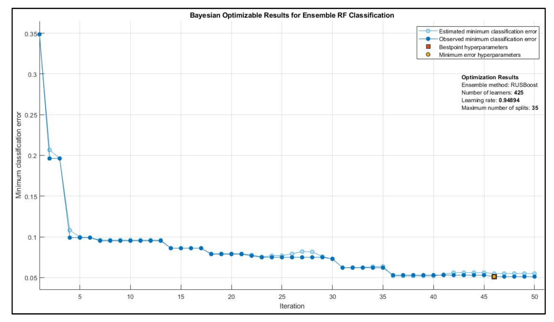
2.7. Estimating Land Suitability Classes Based on Machine Learning

A set of auxiliary variables (i.e., remotely sensed data, geomorphology, and terrain attributes) and RF as a base classifier for RUSBoost ensemble classification technique was used to predict the spatial distribution of land suitability classes for sugar beet. The random forest (RF) machine learning model was selected, due to its successful applications in earlier studies [27,28,29,30,31,32,33] and its relatively good accuracy, robustness, and ease of use. Importantly, it was proved that RF work well when there is no massive availability of data.
Spectral bands and indices derived from the Sentinel-2 satellite, which was acquired on 4 March 2020, were used as auxiliary variables for predicting land suitability class: spectral bands (SENTINEL-2 10 m spatial resolution bands: B2 (490 nm), B3 (560 nm), B4 (665 nm), and B8 (842 nm), and SENTINEL-2 20 m spatial resolution bands: B5 (705 nm), B6 (740 nm), B7 (783 nm), B8a (865 nm), B11 (1610 nm) and B12 (2190 nm)), normalized deference vegetation index (NDVI, [34]), and soil adjusted vegetation index (SAVI, [35]). The auxiliary variables are all co-registered to the same 10 m raster grid with a size of 10 m as the main variables.
Geomorphology maps are valuable auxiliary data since they provide information such as soil parent material and genesis [27,31,36,37].
Terrain attributes, including elevation, slope, aspect, length–slope factor (LS factor), valley depth, topographic wetness index (TWI), analytical hillshading, channel network base level, channel network distance, closed depressions, convergence index, plan curvature, profile curvature, relative slope position, total catchment area, the multi-resolution index of valley bottom flatness (MrVBF), and multi-resolution ridge top flatness (MrRTF) were extracted and computed through a digital elevation model (DEM), ALOS Global Digital Surface Model, downloaded in 17 October 2021, online from https://www.eorc.jaxa.jp/ with a 30 m grid cell resolution and resampled to 10 m spatial resolution using terrain analysis model in SAGA GIS software (system for automated geoscientific analysis) [15].
While constructing a machine learning model, it is almost rare that all of the variables in the dataset are relevant to build a model. Adding redundant variables decreases the model’s generalizability and may also reduce the classifier’s overall accuracy. Identifying only the most relevant features using “Feature selection” approaches make our model simpler to interpret, reduce the variance of the model, and therefore overfitting, and reduce the computational cost (and time) of training a model. In a data science workflow, RF are frequently used for feature selection. After training an RF model, a summary of the frequency of usage for the variables is generated and given as a measure of the variable’s significance [19,34,38,39].
It is critical to adjust model hyperparameters while developing a machine learning classification model. Model hyperparameters are external to the model, and users should tune them by trial and error until they achieve a low level of error when comparing predictions to the validation dataset. Hyperparameter calibration is crucial for managing the training process and delivering high-quality results [19]. Optimization approaches automate the selection of model hyperparameters rather than requiring manual adjustment. The optimizer uses an optimization technique to try alternative combinations of hyperparameter values in order to reduce the model error, and then returns a model with the optimized hyperparameters. In this paper, we deal with hyperparameters optimization within the context of Bayesian optimization, in which the generalization performance of a learning algorithm is treated as a sample from a Gaussian process (GP). The tractable posterior distribution produced by the GP allows for more effective use of the data collected in prior trials, allowing for better decisions regarding which parameters to attempt next [18,34,38,39].

3. Results

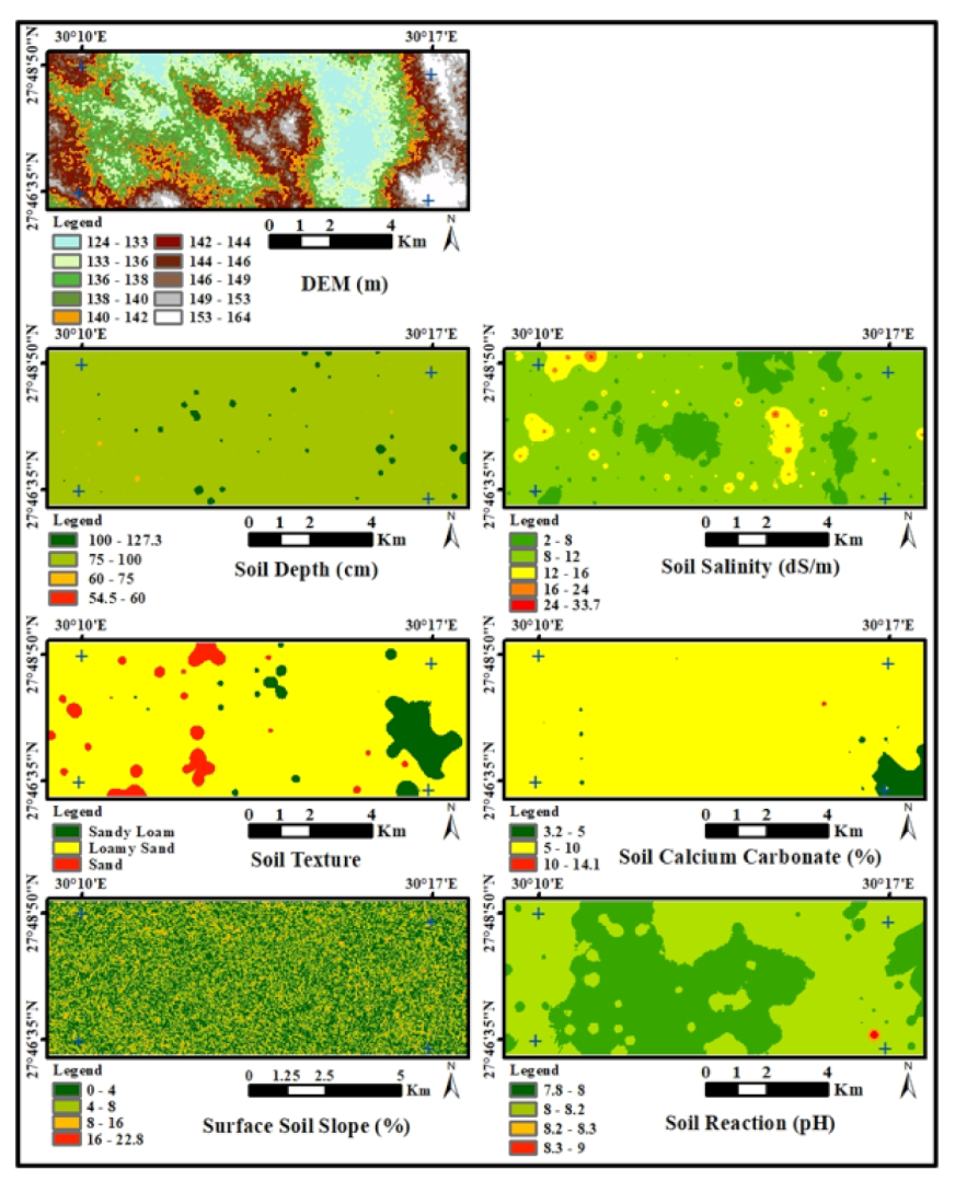
3.1. Land Form of the Study Area

The landscape contains a desert arid region. The soil surface was found to be formed in two units’ shapes; undulated topography and nearly level topography. The texture of these units was found to be loamy sand soil, sandy soil, sandy loam soil (Table 2 and Figure 3).

3.2. Soil Taxonomy

The study area elevated from 124 masl to 164 masl, undulated area with gentle slope of <1. Soil depth ranged from 54.5 cm to 127.3 cm. Soil salinity was found in high (4–8 dS/m) class, occupying around 30% of the total area, while very high salinity (8–16 dS/m) occupied around 60% and the rest of the area was non-saline soil. In total, 90% of the soil texture was loamy sand, 11% was sandy loam and 9% was sandy soil. The soil contained a significant amount of calcium carbonate. Soil pH was particularly apparent from 7.8 to 9 (Figure 3). Soils in the study area were classified according to the Keys to Soil Taxonomy System [40] under two soil orders of Aridisols and Entisols. The studied soils were classified into great group for mapping units. The soil sets of the mapping unit (Figure 4) were the following:
(1)
Aridisols: Typic Haplocalcids, Calcic Haplosalids and Sodic Haplocalcids;
(2)
Entisols: Typic Torrifluvents, Typic Torripsamments and Typic Torriorthents.

3.3. Spatial Variation of Physical and Chemical Criteria

3.3.1. Spatial Variation of the Soil Depth

Deep soil shows a root penetration until below 150 cm for most crops. Soil depth refers to the estimated depth in centimeters to which root growth is unrestricted by any physical or chemical impediment, such as an impenetrable or toxic layer. There are five soil depth classes in the study area namely: very shallow (<30 cm), shallow (30–50 cm), moderately deep (50–100 cm), deep (100–150 cm) and very deep (≥150 cm). The reclassified soil depth map reveals that 99.9% of the study area had moderately deep soil.

3.3.2. Spatial Variation of the Soil Salinity

The distribution pattern of soil salinity in the study area is shown in Table 2 and Figure 3. As it is clear from Figure 3 the slightly saline, moderately saline and saline soils were scattered in the study area and constituted about 12.7%, 80.5% and 6.8 %, respectively.

3.3.3. Spatial Variation of the Soil Texture

Texture is one of the most important soil properties. Most of the physical characteristics of the soil depend upon the type of texture class. There were three textural classes in the study area, namely, sand, loamy sand and sandy loam texture classes. The reclassified soil texture map shows that 4.3%, 88.7% and 7.1% of the study area had sand, loamy sand and sandy loam texture soil, respectively (Figure 5 and Table 3).

3.3.4. Spatial Variation of the Soil CaCO3

The CaCO3 content for the studied soils could be categorized into three classes, as shown in Figure 3 and Table 2. The spatial distribution of CaCO3 shows that 2.8%, 97.1% and 0.1% of the study area was low, slightly and moderately calcareous, respectively.

3.3.5. Spatial Variation of the Soil pH

Soil pH provides the information about the solubility and thus potential availability or phytotoxity of elements for crops and subsequently specifies the soil suitability for a specific crop [41]. The reclassified soil pH map shows that 43.2% and 56.7% of the study area were slightly and medium alkaline (Figure 5 and Table 3).

3.3.6. Spatial Variation of the Slope

The slope of the study area varied between 0% and 16%. The reclassified slope map reveals that slope ranged between 0 and 4 (47.7%), 4 and 8 (44.9%), and >16 (7.4%) as shown in Figure 5 and Table 3.

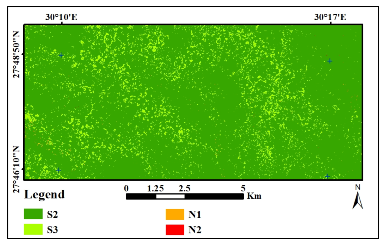
3.4. ML-Based Land Suitability Classes

The processing workflow consists of running the RF as base learner for RUSBoost ensemble classifier and Bayesian optimizer to obtain the best accuracy for the research hypothesis under evaluation using all the auxiliary variables. We used the optimized ML model to measure the importance of different input auxiliary variables as shown in Figure 6.
Based on Figure 6, we decided to ignore variables with an importance of less than 0.3 (slope, aspect, depression area, and catchment area). Then, we repeated the classification process with the reduced auxiliary variables. Figure 7 shows the classification error during the optimization process. Table 4 shows the classification accuracy of the optimized model with the reduced auxiliary variables. The overall accuracy was 94.9%.
Suitability maps were produced based on random forest machine learning model (Figure 8 and Table 5), Multi-criteria approach (Figure 9 and Table 6) were examined and proof to be a high accurate results.
By calculating the coefficient of variation between the two methods, it was found that it was 0.97, which indicates the strength of the correlation between the two methods.
Considering the difference in the two units S1 (0.16%) and N2 (0.04) using the two methods, which could be considered a negligible area, they should be ignored due to their smallness and limitations.

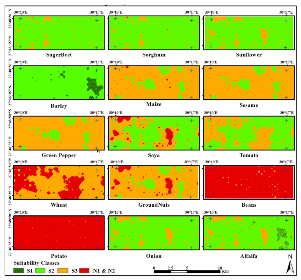
3.5. Description of the Selected Land Use Types

The results indicated that the suitable crops (S2) for the whole area were barley, sorghum, soybean, sugar beet, onion, sunflower, tomato and alfalfa, while the marginally suitable crops (S3) were wheat, maize, green pepper, sesame and groundnut. On the other hand, potato and beans were not suitable for the area under current soil properties as shown in Figure 9.
The government and decision makers in the last few years constructed a new factory in El Minia governorate for extracting sugar from sugar beet. Sugar beet is considered a good crop in the study area, given that it is less demanding than other crops in water consumption, while it is also more salt tolerant, and the cultivation period is shorter than that of sugar cane. Therefore, this land use is considered a promising option in Egypt in general and in El Minia particularly. The total highly suitable area (S1) that could be cultivated by sugar beet in the studied area was 10.8 hectare (0.16%). The S2 soils covered 6111.7 ha (88.1%). The S3 soils covered 810.7 ha (11.7% of the study area. About 2.9 ha (0.04% of the study area) was considered not suitable (N) for sugar beet (Table 7 and Table 8 and Figure 9).
Barley is characterized by the relative ability to resist drought and its high salt tolerance. Therefore, barley is considered more suitable in salty soils. Table 7 and Table 8 and Figure 9 show that the total area of S1 which can be cultivated with barley in the study area was about 471.5 ha (6.8%). Moderately suitable (S2) covered about 6415.3 ha (92.5%). Marginally suitable soils (S3) covered about 46.4 ha (0.67%). The non-suitable soils (N) covered 2.5 ha (0.04%).
Alfalfa is considered a highly profitable cash crop with a high gross margin, being also as a crop that has a preferred residual impact to soil fertility. Alfalfa could be highly suitable (S1) in the study area for about 157.4 ha (2.3%). Moderately suitable soil (S2) was recorded in about 5547.2 ha (80%). Marginally suitable soil (S3) covered about 1229.3 ha (17.7%). A total of 1.7 ha of the study area was classified as non-suitable for alfalfa (Table 7 and Table 8 and Figure 9).
Wheat is the most important cash as well as staple crop in the study area. About 4503.6 ha (64.9% of the area) was found to be marginally suitable for wheat, while 2431.9 ha (35.1% of the area) was found to be not suitable (N) for wheat crop (Table 7 and Table 8 and Figure 9).
Sunflower is considered a highly profitable cash crop with a high gross margin. The land suitability analysis for sunflower indicated that about 5700 ha (82.2%) and 1234 ha (17.8%) of the total area were moderately suitable and marginally suitable, respectively (Table 7 and Table 8 and Figure 9).
Sorghum and soybean are considered relatively resistant to salinity. The land suitability analysis for sorghum indicated that 6111.3 ha (88.1%) and 806.6 ha (11.6%) were moderately suitable and marginally suitable, respectively. On the other hand, 3971.1 ha of land (57.3%) was classified as moderately suitable, 2458.4 ha (35.5%) as marginally suitable and 506.1 ha (7.3%) as not suitable for soybean (Table 7 and Table 8 and Figure 9).
Tomato, sesame and onion are considered the most famous highly profitable cash crops. The land suitability analysis for tomato indicated that 3967.6 ha (57.2%) and 2966.3 ha (42.8% of the total area) were moderately suitable and marginally suitable, respectively. On the other hand, 782.1 ha (11.3%) were classified as moderately suitable, 6151.8 ha (88.7%) as marginally suitable and 506.1 ha (7.3%) of land as not suitable for sesame. Furthermore, 5704.5 ha (82.3%) and 1229.3 ha (17.7% of land) were classified as moderately suitable and marginally suitable for onion, respectively, as illustrated in Table 7 and Table 8 and Figure 9.
The land suitability analysis for green pepper indicated that 807.2 ha (11.6%) and 6126.3 ha (88.3% of the total area) were moderately suitable and marginally suitable, respectively. On the other hand, 781.8 ha (11.3%) was classified as moderately suitable, while 5646.3 ha (81.4%) was marginally suitable, and 507.2 ha (7.3% of land) was not suitable for groundnut. In the end, 782.1 ha (11.9%) and 6116.7 ha (88.2% of total land) were classified as moderately suitable and marginally suitable for maize, respectively (Table 7 and Table 8 and Figure 9).
The land suitability analysis for potato and beans indicated that the study area was not suitable (N) for 6916.9 ha (99.7%) and 6853.5 ha (98.8%), respectively.

4. Discussion

In land suitability studies, methods such as multi-criteria decision-making methods, analytical hierarchy process, crop simulation models and machine learning related methods are the most popular and dynamic [42]. Remote sensing, geostatistics and geographic information systems were also successfully employed for determining land suitability of important crops in other countries [43]. Land suitability mapping using geochemical and spatial analysis methods was also used in cases of soils contaminated with toxic elements [44]. In the present study, we determined optimized land use through integrated land suitability and the GIS approach in the West El-Minia Governorate, Upper Egypt. The method used is suggested as suitable for similar studies in other areas. The digital elevation model (DEM) employed in this study had paramount importance in distinguishing between common landscape units and their associated soil units as well [13,45,46,47,48]. The main geomorphologic units in the study area were high terraces, medium height terraces, and low terraces. High terraces with height of 142 to 164 m were undulating unit to gently undulating relief and their soils were mostly deep. Soils exerted particle size classes of gravelly sand to gravelly sandy loam with clay content ranging from 1.9% to 13.4%. Their salinity level was mostly medium to extremely high (ECe values ranged from 12 dS/m to 33.7 dS/m). The high salinity was considered a result of aridity prevalence and deficit of precipitation in most of the year, with the exception of some sudden flash floods which may take place once every several years. The soils were neutral to alkaline in reaction, as the pH values ranged between 8.2 and 9. Calcium carbonate contents varied from 5% to 14.1% and gypsum content ranged from 2.3% to 7.8%. Medium height terraces with height of 136 to 142 m were gently undulating unit and their soils were deep to very deep. The soils possessed particle size classes of gravelly sand to sandy loam, while clay content varied between 2.3% and 17.4%. All salinity classes were detected from non-saline to extremely saline (ECe values ranged from 8 dS/m to 12 dS/m). The pH values ranged between 8 and 8.2. Calcium carbonate content ranged from 5 to 10% while gypsum content ranged from 2.1 to 13.4%. Low terraces with a height from 124 m to 136 m were almost flat units and their soils were mostly deep and very deep. The soils exhibited particle size classes of gravelly sandy to sandy clay loam and clay content ranged from 6.7% and 20.8%. The salinity levels were medium to saline (ECe values ranged from 2 dS/m to 8 dS/m). The pH values ranged between 7.8 and 8.2. Calcium carbonate contents varied from 3.2% to 5% and gypsum content ranged from 1.3% to 11.7%.
The existence of adequate management of sustainable agriculture, through the employment of resilient commercial and agricultural practices, may play a crucial role in enhancing the resilience of the fragile desert environment. The arid climate in the broader region necessitates taking into consideration also non-renewable factors such as desalination and treated sewage effluent (TSE) for efficiently assessing suitability of irrigated land [49]. Due to the harsh environment of natural vegetation growth, the soil organic matter content is predictably low and affects the soil structure. Therefore, it is desirable to increase OM in soil by adding organic amendments and incorporating plant residues such as leguminous plants into the soil [50]. With regard to soil erosion, mechanical settlement should be avoided to mitigate the potential unfortunate consequences of compaction and soil structure degradation that may exacerbate soil erosion. Agriculture may play an important role for climate change mitigation through storage of C in soil, above and belowground biomass as well as litter [51]. With regard to alkaline soils, it is recommended to use ammonium or potassium sulfate to reduce the alkalinity of the soil. Since the application of management techniques is costly, extensive and conservative practices are recommended to maintain high productivity. In general, the proposed framework will be considered by the research work as a basic reference and strategic guide to identify potential flaws and increase the possibility of progress.
In connection with the assessment of the potential of soil resources, the most severe limitations were coarse texture, medium grain content, followed by limited depth and poor internal drainage. While saturation with carbonate and sodium were the least influential, they were generally not related to the specific soil mapping unit. So, it is recommended to design a good land management system to overcome some of the temporarily limiting factors that may hinder optimal agricultural use.
Crop production needs to identify the soil factors that limit the cultivation process in the study area. It was found that these factors were slope, surface rockiness, erosion, light texture and reduced soil fertility [12,45,46,47,48]. Statistical analysis showed that the results of the proposed model were highly consistent with the actual crop requirements. In this regard, appropriate modeling presents a flexible technique that contributes to improving the assessment of land suitability for crops in newly reclaimed areas, making it more accurate and reliable, thus assisting decision makers in their selection among different types of land use due to the ability to adjust the weights of the assessment criterion as per the requirements of the selected crops. The proposed model provides a significant improvement in the assessment of land suitability for the newly reclaimed desert lands, resulting in the addition of new areas to the agricultural production sector.
The output of the research concluded that potato and beans have the lowest suitability class N with areas of 6916.8 ha (99.73%) and 6853.4 ha (98.82%), respectively, while for S2 classes were barley, alfalfa, onion, sorghum, sugar beet, soybean, sunflower and tomato with areas of 6415.3 ha (92.5%), 5547.2 ha (80%), 5704.5 ha (82.3%) 6111.3 ha (88.1%), 6111.3 ha (88.1%), 3971.1 ha (57.3%), 5700 ha (82.2%), and 3967.6 ha (57.2%), respectively. Meanwhile, S3 classes occupied areas of 6126.3 ha (88.3%), 5646.3 ha (81.4%), 6116.7 ha (88.2%), 6151.8 ha (88.7%) and 4503.6 ha (64.9%) for green pepper, groundnut, maize, sesame and wheat, respectively. Replanting a particular crop in the same site causes an increase in pests at that site, especially soil pests or pests that infect certain varieties and types of vegetables [52]. So, we could easily overcome many pests if we avoid planting the garden or field with the same crop or crops that are affected by the same pests for a period of two to three years, as that period is sufficient to eliminate most pathogens, given the absence of their host [53]. The absence of a host for many insects causes their elimination, especially those that move slowly from one field to another, in search of their hosts, as most insects cannot live for a long time in the absence of their hosts [35]. Moreover, crop rotation reduces the incidence of viral diseases caused by viruses present in the soil, as these diseases may be transmitted mechanically to plants [53]. In general, crop rotation contributes to the treatment of soil and the control of pests and plant diseases, and it means the succession of agricultural crops based on a scientific basis, by changing the type of crop planted on a particular plot of land from one season to another, with the aim of reducing the spread of pests, as the cycle works to interrupt the cycle of the life of the insect before its completion, thus eliminating the pathogen [52,53,54]. The agricultural cycle contributes to maintaining the balance of nutrients and fertilizer in the soil; some vegetable crops prefer a higher percentage of nitrogen, phosphorous and potassium, so these vegetables need animal fertilizer. While root crops do not grow well in animal manure, they remain dwarfed and distorted. Therefore, it is preferable not to plant root crops immediately after planting crops that need animal manure, or not plant it for one or two seasons, after a group of crops that grow well with animal manure on the same plot of land [55,56,57,58].
In this study, while selecting this practice for the agricultural cycle, it was necessary to pay attention to the following matters: (1) It is preferable not to reuse a particular site to grow the same type of plants that were planted on it in the previous season or in recent seasons, especially when growing seasonal plants, such as vegetables and medicinal herbs, or when replanting perennial trees, such as fruit trees and shrubs [56,59,60,61]. (2) The ideal practice is to plant different types and varieties of seasonal crops in different locations and basins, and not to replant the same crop in the same location or basin until after a few years, as this practice helps in controlling harmful and vascular insects. Crop rotation also eliminates weeds and maintains soil fertility and good levels of organic matter [55,56,57,58,59,60,61]. Crops that are similar in their predisposition to the same diseases, and in their susceptibility to harmful insects, should be planted at spaced intervals [62,63,64,65]. (3) Close alternation between plantings is always preferred to reduce the periods of time during which the soil remains free of vegetation cover [66,67,68]. (4) Apply a short agricultural cycle in the limited agricultural area while maintaining a healthy soil structure [69,70,71,72]. (5) If it is not possible to practice crop rotation, for practical reasons, it should partially compensate for it through interlacing and intercropping, provided that healthy soils are maintained [62,63,64,65,66,67,68,69,70,71,72]. (6) In the framework of a crop rotation system, before replanting plants of the same species in the same site, it must be ensured that the soil is free of germs and associated parasitic plants [56,59,60,61]. The agricultural pattern of growing the same family of vegetables annually on the same plot of land to meet market demands is a good example of poor or non-successive crops rotations. Thus, it causes severe depletion of the land as well as exacerbation of soil pests. Thus, many fungal, bacterial, insect and parasitic diseases can be combated through proper agricultural rotation on the one hand and mixed and intercropping cultivation on the other. Additionally, it will maintain soil fertility in the short term and maintain soil quality in the long term, which will raise the production capability and raise the degree of soil suitability for different crops.
In general, it is preferable to follow the triple cycle, that is, between three types of crops, in one plot of land. For example, oil crops are exchanged in a three-year cycle, and include two types of grains, such as wheat and corn, taking into account that sunflowers are not planted in the land affected by white rot, for a period of not less than seven years. It could be also applied a quadrilateral cycle, that is, between four types of crops, on the same plot of land—for example, planting chickpeas and peas in the first year, and then, in the next three years, plant leafy and flowering vegetables, such as cauliflower, cabbage and beetroot, in the second year. In the third year, fruit crops such as tomatoes and peppers are planted, and finally, in the fourth year, we plant root crops such as carrots, beets and onions. All this succession between crops is in consideration of the fact that sugar beet is the main crop in the land every year.

5. Conclusions

The study aimed to spotlight and analyze the affecting factors on the efficiency of beet sugar economic producing and manufacturing. Our results suggested the importance of raising the sugar beet cultivated area, as it is considered a profitable crop and favorable to soil properties and it could be cultivated at the first stages of reclamation. The present paper also recommends enabling and activating the role of agriculture guidance to raise the cultivated area and acre productivity of sugar beet, encouraging and putting incentives for investors to work and invest at the field of sugar beet manufacturing. This study aimed to classify lands with different degrees of suitability as an index to help decision makers and farmers, especially where crop selection is considered to be an important component of management. The output of the research concluded that potato and beans have the lowest suitability class N, while for S2 classes were barley, alfalfa, onion, sorghum, sugar beet, soybean, sunflower and tomato. Meanwhile S3 classes were dominant for green pepper, groundnut, maize, sesame and wheat. The assessment of the physical land suitability of the study area indicates that it has huge potential for sugar beet, barley, sorghum, soybean, sunflower and tomato production. This paper proves that GIS is a powerful tool in highlighting the agricultural land suitability and analyzing the cross tabulation between various thematic map classes with respect to agricultural land suitability and can be applied at various scales. Our results also confirmed the ability of GIS as a tool for saving time and reducing costs, which would be useful for policy makers and growers.

Supplementary Materials

The following are available online at https://www.mdpi.com/article/10.3390/su132112236/s1, Tables S1–S15: Land use requirements for the main crops.

Author Contributions

Conceptualization, Y.M.Z., M.M.M., M.A.E.A., M.R.M. and G.K.; methodology Y.M.Z., M.M.M., M.A.E.A. and M.R.M.; software, M.A.E.A. and G.K.; validation, Y.M.Z., M.M.M. and M.A.E.A.; formal analysis, Y.M.Z., M.M.M. and M.A.E.A.; investigation, Y.M.Z., M.M.M. and M.A.E.A.; resources, Y.M.Z., M.M.M., M.A.E.A. and M.R.M.; data curation, Y.M.Z., M.M.M., M.A.E.A. and G.K.; writing—original draft preparation, Y.M.Z., M.M.M., M.A.E.A. and G.K.; writing—review and editing, Y.M.Z., M.M.M., M.A.E.A. and G.K.; visualization, M.A.E.A. and G.K.; supervision, Y.M.Z., M.M.M. and M.A.E.A.; project administration, Y.M.Z., M.M.M., M.A.E.A. and G.K.; funding acquisition, Y.M.Z. All authors have read and agreed to the published version of the manuscript and all authors confirm that all the text of this paper is new and has not been published previously.

Funding

This research received no external funding.

Institutional Review Board Statement

Not applicable.

Informed Consent Statement

Not applicable.

Data Availability Statement

Data is available by the authors upon request.

Acknowledgments

The authors would like to thank the Faculty of Agriculture Ain Shams University, Egypt, for laboratory analysis. The authors would like to thank National Authority for Remote Sensing and Space Sciences, Cairo, Egypt, and Institute of Olive Tree, Subtropical Crops and Viticulture, Chania, Greece. The authors would like to thank the Canal Sugar Company and Yasser M. Zakarya, for their assistance in the field work.

Conflicts of Interest

The authors declare no conflict of interest.

References

  1. AbdelRahman, M.A.E.; Natarajan, A.; Hegde, R. Assessment of land suitability and capability by integrating remote sensing and GIS for agriculture in Chamarajanagar district, Karnataka, India. Egypt. J. Remote Sens. Space Sci. 2016, 19, 125–141. [Google Scholar] [CrossRef] [Green Version]
  2. AbdelRahman, M.A.E.; Natarajan, A.; Srinivasamurthy, C.A.; Hegde, R. Estimating soil fertility status in physically degraded land using GIS and remote sensing techniques in Chamarajanagar district, Karnataka, India. Egypt. J. Remote Sens. Space Sci. 2016, 19, 95–108. [Google Scholar] [CrossRef] [Green Version]
  3. Mu, Y. Developing a suitability index for residential land use: A case study in Dianchi Drainage Area. Master’s Thesis, University of Waterloo, Waterloo, ON, Canada, 2006. [Google Scholar]
  4. He, Y.; Yao, Y.; Chen, Y.; Ongaro, L. Regional land suitability assessment for tree crops using remote sensing and GIS. In Proceedings of the IEEE Computer Distributed Control and Intelligent Environmental Monitoring (CDCIEM), Changsha, China, 19–20 February 2011; pp. 354–363. [Google Scholar]
  5. Beek, K.J.; De Bie, K.; Driessen, P. Land information and land evaluation for land use planning and sustainable land management. Land 1997, 1, 27–44. [Google Scholar]
  6. Merolla, S.; Armesto, G.; Calvanese, G. A GIS application for assessing agricultural land. ITC J. 1994, 1994, 264–269. [Google Scholar]
  7. Ali, R.R.; El-Kader, A.A.A.; Essa, E.F.; AbdelRahman, M.A.E. Application of remote sensing to determine spatial changes in soil properties and wheat productivity under salinity stress. Plant Arch. 2019, 19, 616–621. [Google Scholar]
  8. Rhoades, J.D.; Kandiah, A.; Mashali, A.M. The Use of Saline Waters for Crop Production; FAO Irrigation and Drainage Paper 48; FAO: Rome, Italy, 1992; Volume 133, pp. 52–67. [Google Scholar]
  9. Sys, C.; Van Ranst, E.; Debaveye, J. Land Evaluation. Part I: Principles in Land Evaluation and Crop Production Calculations; Agricultural Publication No. 7; GADC: Brussels, Belgium, 1991. [Google Scholar]
  10. AbdelRahman, M.A.E.; Arafat, S.M. An approach of agricultural courses for soil conservation based on crop soil suitability using geomatics. Earth Syst. Environ. 2020, 4, 273–285. [Google Scholar] [CrossRef]
  11. Bandyopadhyay, S.; Jaiswal, R.K.; Hegde, V.S.; Jayaraman, V. Assessment of land suitability potentials for agriculture using a remote sensing and GIS based approach. Int. J. Remote Sens. 2009, 30, 879–895. [Google Scholar] [CrossRef]
  12. Pan, G.; Pan, J. Research in crop land suitability analysis based on GIS. In Proceedings of the International Conference on Computer and Computing Technologies in Agriculture, Beijing, China, 29–31 October 2011; Springer: Berlin/Heidelberg, Germany, 2011; pp. 314–325. [Google Scholar]
  13. AbdelRahman, M.A.E.; Natarajan, A.; Hegde, R.; Prakash, S.S. Assessment of land degradation using comprehensive geostatistical approach and remote sensing data in GIS-model builder. Egypt. J. Remote Sens. Space Sci. 2019, 22, 323–334. [Google Scholar] [CrossRef]
  14. AbdelRahman, M.A.E.; Shalaby, A.; Essa, E.F. Quantitative land evaluation based on fuzzy-multi-criteria spatial model for sustainable land-use planning. Model. Earth Syst. Environ. 2018, 4, 1341–1353. [Google Scholar] [CrossRef]
  15. Dif, A.E.A. An Economic Study about Beet Sugar Manufacturing and Producing at Sharkia Governorate. Egypt. J. Agric. Econ. 2016, 26, 395–404. [Google Scholar]
  16. Taghizadeh-Mehrjardi, R.; Nabiollahi, K.; Rasoli, L.; Kerry, R.; Scholten, T. Land Suitability Assessment and Agricultural Production Sustainability Using Machine Learning Models. Agronomy 2020, 10, 573. [Google Scholar] [CrossRef]
  17. AL-Shdaifat, E.; Al-hassan, M.; Aloqaily, A. Effective heterogeneous ensemble classification: An alternative approach for selecting base classifiers. ICT Express 2020, 7, 342–349. [Google Scholar] [CrossRef]
  18. Seiffert, C.; Khoshgoftaar, T.M.; Hulse, J.V.; Napolitano, A. RUSBoost: Improving classification performance when training data is skewed. In Proceedings of the 2008 19th International Conference on Pattern Recognition, Tampa, FL, USA, 8–11 December 2008; pp. 1–4. [Google Scholar]
  19. Snoek, J.; Larochelle, H.; Adams, R.P. Practical Bayesian Optimization of Machine Learning Algorithms. Adv. Neural Inf. Process. Syst. 2012, 25, 2951–2959. [Google Scholar]
  20. Khaledian, Y.; Miller, B.A. Selecting appropriate machine learning methods for digital soil mapping. Appl. Math. Model. 2020, 81, 401–418. [Google Scholar] [CrossRef]
  21. Kornblyu, E.A.; Smirnova, S.F. FAO Guidelines for Soil Profile Description. Sov. Soil Sci.-USSR 2006, 2, 762. [Google Scholar]
  22. Sys, C.; Van Ranst, E.; Debavey, J.; Beernaert, F. Land Evaluation, Part III Crop Requirements; Agricultural Publication No. 7; General Administration for Development Cooperation: Gheut, Belgium, 1993. [Google Scholar]
  23. Zakarya, Y.M. Land Resources Assessment Using GIS, Expert Knowledge and Remote Sensing in the Desert Environment. Ph.D. Thesis, Faculty of Agriculture, Ain Shams University, Cairo, Egypt, 2009. [Google Scholar]
  24. AbdelRahman, M.A.E.; Zakarya, Y.M.; Metwaly, M.M.; Koubouris, G. Deciphering Soil Spatial Variability through Geostatistics and Interpolation Techniques. Sustainability 2021, 13, 194. [Google Scholar] [CrossRef]
  25. Yao, X.; Fu, B.; Lü, Y.; Sun, F.; Wang, S.; Liu, M. Comparison of four spatial interpolation methods for estimating soil moisture in a complex terrain catchment. PLoS ONE 2013, 8, e54660. [Google Scholar] [CrossRef]
  26. Metwaly, M.M. Sustainable Land use Planning of El-Qaa Plain, South Sinai, Egypt. J. Soil Sci. Agric. Eng. 2013, 2, 227–238. [Google Scholar]
  27. Behrens, T.; Schmidt, K.; Zhu, A.-X.; Scholten, T. The ConMap approach for terrain-based digital soil mapping. Eur. J. Soil Sci. 2010, 61, 133–143. [Google Scholar] [CrossRef]
  28. Nabiollahi, K.; Golmohammadi, F.; Taghizadeh-Mehrjardi, R.; Kerry, R. Assessing the e_ects of slope gradient and land use change on soil quality degradation through digital mapping of soil quality indices and soil loss rate. Geoderma 2018, 318, 482–494. [Google Scholar] [CrossRef]
  29. Nabiollahi, K.; Taghizadeh-Mehrjardi, M.; Eskandari, S. Assessing and monitoring the soil quality of forested and agricultural areas using soil-quality indices and digital soil-mapping in a semi-arid environment. Arch. Agron. Soil Sci. 2018, 64, 482–494. [Google Scholar] [CrossRef]
  30. Nabiollahi, K.; Eskandari, S.; Taghizadeh-Mehrjardi, R.; Kerry, R.; Triantafilis, J. Assessing soil organic carbon stocks under land use change scenarios using random forest models. Carbon Manag. 2019, 10, 63–77. [Google Scholar] [CrossRef]
  31. Taghizadeh-Mehrjardi, M.; Nabiollahi, K.; Minasny, B.; Triantafilis, J. Comparing data mining classifiers to predict spatial distribution of USDA-family soil groups in Baneh region, Iran. Geoderma 2015, 253, 67–77. [Google Scholar] [CrossRef]
  32. Taghizadeh-Mehrjardi, M.; Nabiollahi, K.; Kerry, R. Digital mapping of soil organic carbon at multiple depths using di_erent data mining techniques in Baneh region, Iran. Geoderma 2016, 266, 98–110. [Google Scholar] [CrossRef]
  33. Pahlavan-Rad, M.R.; Toomanian, N.; Khormali, F.; Brungard, C.W.; Komaki, C.B.; Bogaert, P. Updating soil survey maps using random forest and conditioned Latin hypercube sampling in the loess derived soils of northern Iran. Geoderma 2014, 232, 97–106. [Google Scholar] [CrossRef]
  34. Freden, S.C.; Mercanti, E.P.; Becker, M.A. (Eds.) Third Earth Resources Technology Satellite-1 Symposium; NASA Science and Technology Information: Washington, DC, USA, 1973; Volume 1, pp. 309–317.
  35. Huete, A.A. Soil-adjusted vegetation index (SAVI). Remote Sens. Environ. 1988, 25, 295–309. [Google Scholar] [CrossRef]
  36. Taghizadeh-Mehrjardi, R.; Sarmadian, F.; Minasny, B.; Triantafilis, J.; Omid, M. Digital mapping of soil classes using decision tree and auxiliary data in the Ardakan region, Iran. Arid Land Res. Manag. 2014, 213, 15–28. [Google Scholar] [CrossRef]
  37. Zeraatpisheh, M.; Ayoubi, S.; Jafari, A.; Finke, P. Comparing the e_ciency of digital and conventional soil mapping to predict soil types in a semi-arid region in Iran. Geomorphology 2017, 285, 186–204. [Google Scholar] [CrossRef]
  38. Olaya, V.A. Gentle Introduction to SAGA GIS; The SAGA User Group eV: Gottingen, Germany, 2004; p. 216. [Google Scholar]
  39. Rouse, J.W.; Hass, R.H.; Schell, J.A.; Deering, D.W. Monitoring vegetation systems in the Great Plains with ERTS. In Technical Presentations Section A Proceedings of the NASA SP-351; Third Earth Resources Technology Satellite-Symposium; NASA Special Publication: Washington, DC, USA, 1973. [Google Scholar]
  40. USDA. Keys to Soil Taxonomy, 11th ed.; The U.S. Department of Agriculture: Washington, DC, USA, 2003.
  41. Halder, J.C. Land suitability assessment for crop cultivation by using remote sensing and GIS. J. Geogr. Geol. 2013, 5, 65. [Google Scholar] [CrossRef]
  42. Mugiyo, H.; Chimonyo, V.G.P.; Sibanda, M.; Kunz, R.; Masemola, C.R.; Modi, A.T.; Mabhaudhi, T. Evaluation of Land Suitability Methods with Reference to Neglected and Underutilised Crop Species: A Scoping Review. Land 2021, 10, 125. [Google Scholar] [CrossRef]
  43. Trigoso, D.I.; López, R.S.; Briceño, N.B.R.; López, J.O.S.; Fernández, D.G.; Oliva, M.; Huatangari, L.Q.; Murga, R.E.T.; Castillo, E.B.; Gurbillón, M.Á.B. Land Suitability Analysis for Potato Crop in the Jucusbamba and Tincas Microwatersheds (Amazonas, NW Peru): AHP and RS–GIS Approach. Agronomy 2020, 10, 1898. [Google Scholar] [CrossRef]
  44. Alexakis, D.E.; Bathrellos, G.D.; Skilodimou, H.D.; Gamvroula, D.E. Land Suitability Mapping Using Geochemical and Spatial Analysis Methods. Appl. Sci. 2021, 11, 5404. [Google Scholar] [CrossRef]
  45. Azzam, M.A. Land suitability evaluation for cultivation of some soils in western desert of egypt, el-minya governorate using gis and remote sensing. Int. J. Adv. Res. 2016, 4, 486–503. [Google Scholar]
  46. Yossif, H.; Taher, M. Soil Classification and Optimum Agricultural Use for Some Areas at the Western Desert Fringe, El-Minia Governorate, Egypt. Alex. Sci. Exch. J. 2020, 41, 317–340. [Google Scholar] [CrossRef]
  47. Rashed, H.S.A. Classification and Mapping of Land Productivity, Capability and Suitability for Production Crops in West El-Minia Governorate, Egypt. J. Soil Sci. Agric. Eng. 2020, 11, 709–717. [Google Scholar]
  48. Mohamed, A.H.; Shendi, M.M.; Awadalla, A.A.; Mahmoud, A.G.; Semida, W.M. Land suitability modeling for newly reclaimed area using GIS-based multi-criteria decision analysis. Environ. Monit. Assess. 2019, 191, 1–13. [Google Scholar] [CrossRef]
  49. Aldababseh, A.; Temimi, M.; Maghelal, P.; Branch, O.; Wulfmeyer, V. Multi-criteria evaluation of irrigated agriculture suitability to achieve food security in an arid environment. Sustainability 2018, 10, 803. [Google Scholar] [CrossRef] [Green Version]
  50. Michalopoulos, G.; Kasapi, K.A.; Koubouris, G.; Psarras, G.; Arampatzis, G.; Hatzigiannakis, E.; Kavvadias, V.; Xiloyannis, C.; Montanaro, G.; Malliaraki, S. Adaptation of Mediterranean olive groves to climate change through sustainable cultivation practices. Climate 2020, 8, 54. [Google Scholar] [CrossRef] [Green Version]
  51. Montanaro, G.; Amato, D.; Briglia, N.; Russo, C.; Nuzzo, V. Carbon Fluxes in Sustainable Tree Crops: Field, Ecosystem and Global Dimension. Sustainability 2021, 13, 8750. [Google Scholar] [CrossRef]
  52. Hamadttu, A.F.E. Insect Pest Management in Organic Farming System, Multifunctionality and Impacts of Organic and Conventional Agriculture; Moudrý, J., Mendes, K.F., Bernas, J., da Teixeira, R.S., de Sousa, R.N., Eds.; IntechOpen: London, UK, 2019. [Google Scholar]
  53. Blake, L. Protection and Pest Management; Extension Implementation Program Grant No. 2017-70006-27200/Project Accession No. 1014037; The USDA National Institute of Food and Agriculture: Washington, DC, USA, 2019.
  54. Alyokhin, A.; Nault, B.; Brown, B. Soil conservation practices for insect pest management in highly disturbed agroecosystems—A review; Special Issue: Insects in Agroecosystems, The Netherlands Entomological Society. Entomol. Exp. Appl. 2020, 168, 7–27. [Google Scholar] [CrossRef]
  55. Leteinturier, B.; Herman, J.; Longueville, F.D.; Quintin, L.; Oger, R. Adaptation of a crop sequence indicator based on a land parcel management system. Agric. Ecosyst. Environ. 2006, 112, 324–334. [Google Scholar] [CrossRef]
  56. Singha, C.; Swain, K.C. Land Suitability Evaluation Criteria for Agricultural crop selection: A Review. Agric. Rev. 2016, 37, 125–132. [Google Scholar] [CrossRef] [Green Version]
  57. Lenz-Wiedemann, V.I.S.; Klar, C.W.; Schneider, K. Development and test of a crop growth model for application within a Global Change decision support system. Ecol. Model. 2010, 221, 314–329. [Google Scholar] [CrossRef]
  58. Lorenz, M.; Fürst, C.; Thiel, E. A methodological approach for deriving regional crop rotations as basis for the assessment of the impact of agricultural strategies using soil erosion as example. J. Environ. Manag. 2013, 127, S37–S47. [Google Scholar] [CrossRef]
  59. Abuzaid, A.S.; Jahin, H.S.; Asaad, A.A.; Fadl, M.E.; AbdelRahman, M.A.E.; Scopa, A. Accumulation of Potentially Toxic Metals in Egyptian Alluvial Soils, Berseem Clover (Trifolium alexandrinum L.), and Groundwater after Long-Term Wastewater Irrigation. Agriculture 2021, 11, 713. [Google Scholar] [CrossRef]
  60. Abuzaid, A.S.; AbdelRahman, M.A.E.; Fadl, M.E.; Scopa, A. Land Degradation Vulnerability Mapping in a Newly-Reclaimed Desert Oasis in a Hyper-Arid Agro-Ecosystem Using AHP and Geospatial Techniques. Agronomy 2021, 11, 1426. [Google Scholar] [CrossRef]
  61. AbdelRahman, M.A.E.; Rehab, H.H.; Yossif, T.M.H. Soil fertility assessment for optimal agricultural use using remote sensing and GIS technologies. Appl. Geomat. 2021. [Google Scholar] [CrossRef]
  62. Mahmoudzadeh, H.; Matinfar, H.R.; Taghizadeh-Mehrjardi, R.; Kerry, R. Spatial prediction of soil organic carbon using machine learning techniques in western Iran. Geoderma Reg. 2020, 21, e00260. [Google Scholar] [CrossRef]
  63. Waldhoff, G.; Lussem, U.; Bareth, G. Multi-data approach for remote sensing-based regional crop rotationmapping: A case study for the Rur catchment, Germany. Int. J. Appl. Earth Obs. Geoinf. 2017, 61, 55–69. [Google Scholar] [CrossRef]
  64. Jayanth, J.; Aravind, R.; Amulya, C.M. Classification of Crops and Crop Rotation Using Remote Sensing and GIS-Based Approach: A Case Study of Doddakawalande Hobli, Nanjangudu Taluk. J. Indian Soc. Remote Sens. 2021. [Google Scholar] [CrossRef]
  65. Schönhart, M.; Schmid, E.; Schneider, U.A. CropRota—A crop rotation model to support integrated land use assessments. Eur. J. Agron. 2011, 34, 263–277. [Google Scholar] [CrossRef]
  66. Waldhoff, G.; Curdt, C.; Hoffmeister, D.; Bareth, G. Analysis of multitemporal and multisensor remote sensing data for crop rotation mapping. ISPRS Ann. Photogramm. Remote Sens. Spat. Inf. Sci. 2012, 1, 177–182. [Google Scholar] [CrossRef] [Green Version]
  67. Hütt, C.; Koppe, W.; Miao, Y.; Bareth, G. Best accuracy land use/land cover (LULC) classification to derive crop types using multitemporal, multisensor, and multi-polarization SAR satellite images. Remote Sens. 2006, 8, 684. [Google Scholar] [CrossRef] [Green Version]
  68. Waldner, F.; Canto, G.S.; Defourny, P. Automated annual cropland mapping using knowledge-based temporal features. ISPRS J. Photogramm. Remote Sens. 2015, 110, 1–13. [Google Scholar] [CrossRef]
  69. Wilson, H.M.; Al-Kaisi, M.M. Crop rotation and nitrogen fertilization effect on soil CO2 emissions in central Iowa. Appl. Soil Ecol. 2008, 39, 264–270. [Google Scholar] [CrossRef]
  70. Casasnovas, M.J.; Martin-Monetero, A.; Casterad, M.A. Mapping multi-year cropping patterns in small irrigation districts from time series analysis of Landsat TM images. Eur. J. Agron. 2005, 23, 159–169. [Google Scholar] [CrossRef]
  71. Jamil, M.; Sajjad, H. Deriving cropping system efficiency pattern using remote sensing and GIS: A case study of Bijnor district, India. Int. J. Adv. Remote Sens. GIS Geogr. 2016, 4, 27–40. [Google Scholar]
  72. Blaes, L.; Vanhalle, P. Defourny Efficiency of crop identification based on optical and SAR image time series. Remote Sens. Environ. 2005, 96, 352–365. [Google Scholar] [CrossRef]
Figure 1. Location of the study area.
Sustainability 13 12236 g001
Figure 2. Methodology flowchart; (A) flowchart for suitability process, (B) process steps for land suitability model.
Sustainability 13 12236 g002
Figure 3. Landform of the study area associated with the soil profile location.
Sustainability 13 12236 g003
Figure 4. The units of the soil taxonomy map are shown at the family level in the study area.
Sustainability 13 12236 g004
Figure 5. Soil characteristics of the study area.
Sustainability 13 12236 g005
Figure 6. Auxiliary variables importance for machine learning–based land suitability evaluation.
Sustainability 13 12236 g006
Figure 7. The empirical performance of the Bayesian optimization process, where the optimizer searches for the set of hyperparameters of ensemble classifier that minimize classification error. The output is the ensemble classifier with the minimum estimated cross-validation error.
Sustainability 13 12236 g007
Figure 8. Suitability map based on random forest machine learning model illustrates the predicted suitability classes of the study area.
Sustainability 13 12236 g008
Figure 9. Soil suitability of the study area.
Sustainability 13 12236 g009
Table 1. Climate features of El-Minia Governorate for a period of 30 years (1975–2005), according to El-Minia meteorological station.
MonthAverage Temperature °CRainfall mmRelativeEvaporation mm/DayWind Speed (Knots)
Mean Temp. °CMin °CMax °CHumidity %
January11.94.620.41.16544.7
February13.55.6221.758.85.45.4
March16.98.625.43.453.97.26.6
April21.912.830.90.544.910.97.2
May26.317.2351.439.113.87.8
June28.519.936.7041.814.68.6
July29.221.136.9048.412.66.2
August28.62136.2052.810.55.6
September26.919.434.7053.19.96.8
October23.316.131.2056.98.15.8
November17.710.725.93.563.45.24.9
December13.16.121.42.167.53.54.1
Mean21.4813.5929.721.1453.88.86.14
Source: Climatological Normals, El-Minia meteorological station, A.R.E., (2011).
Table 2. Landform unit descriptions and statistics.
Landform UnitArea
(Hectare)(%)
Loamy sand soil, Undulated topography3019.2231.63
Loamy sand soil, Nearly level topography2058.6721.57
Sandy soil, Nearly level topography1224.5712.83
Sandy loam soil, Undulated topography3242.7933.97
Table 3. Spatial variation of the physical and chemical criteria.
ECe
(dS/m)
Area
(Hectare)(%)
2–8872.9512.65
8–125558.1980.55
12–16469.366.80
16–2433.940.49
24–33.71.190.02
pHArea
(Hectare)(%)
7.8–82993.6143.20
8–8.23926.2856.66
8.2–8.310.090.15
8.3–95.640.08
Slope
(%)
Area
(Hectare)(%)
0–43319.8647.72
4–83121.6444.87
8–16515.917.42
16–22.81.690.02
Soil Depth
(cm)
Area
(Hectare)(%)
54.5–600.060.00
60–758.780.13
75–1006835.7599.87
100–127.391.031.33
CaCO3
(%)
Area
(Hectare)(%)
3.2–5194.302.80
5–106739.4897.17
10–14.11.840.03
TextureArea
(Hectare)(%)
S295.134.27
LS6127.6488.65
SL489.427.08
Table 4. The classification accuracy of the optimized model.
Predicted Class
True Class Class N2Class N1Class S3Class S2
Class N2100.00%
Class N1 100.00%
Class S2 86.90%7.60%
Class S2 13.10%92.40%
Table 5. Machine learning predicted suitability classes for sugar beet.
Suitability ClassArea
(Hectare)(%)
S28755.4792.15
S3737.197.76
N18.290.09
N20.570.01
Table 6. Traditional suitability method for sugar beet.
Suitability ClassArea
(Hectare)(%)
S110.770.16
S26111.2788.11
S3810.7211.69
N2.880.04
Table 7. Soil suitability classes area in hectare area and percent of the total area.
CropsAreaSoil Suitability Classes
S1S2S3N1
Alfalfa(Hectare)157.395547.231229.311.69
(%)2.2779.9817.720.02
Barely(Hectare)471.456415.3046.382.50
(%)6.8092.500.670.04
Beans(Hectare)-0.4781.676853.48
(%)-0.011.1898.82
Green pepper(Hectare)0.47807.166126.311.69
(%)0.0111.6488.330.02
Groundnut(Hectare)0.31781.815646.28507.22
(%)0.0011.2781.417.31
Maize(Hectare)0.02782.116116.6736.83
(%)0.0011.2888.190.53
Onion(Hectare)0.145704.481229.311.69
(%)0.0082.2517.720.02
Potato(Hectare)-1.0317.736916.86
(%)-0.010.2699.73
Sesame(Hectare)-782.136151.811.69
(%)-11.2888.700.02
Sorghum(Hectare)10.776111.27806.636.97
(%)0.1688.1111.630.10
Soya(Hectare)0.083971.082458.38506.09
(%)0.0057.2635.457.30
Sugar beet(Hectare)10.776111.27810.722.88
(%)0.1688.1111.690.04
Sunflower(Hectare)-5699.951233.981.69
(%)-82.1817.790.02
Tomato(Hectare)-3967.642966.301.69
(%)-57.2142.770.02
Wheat(Hectare)-0.094503.642431.89
(%)-0.0064.9335.06
Table 8. Suggested crops for agricultural rotation in the study area.
No.Crop NameSpeciesPlanting DatePlanting
Period
(Months)
Selected Suitability
Performance
1Sugar beetBeta vulgarisAug.–Sep.–Mid. Oct.6–7S2 > S3
2SorghumSorghum bicolorMid. Apr.4S2 > S3
3SunflowerHelianthus annuusApr.–Jun.3S2 > S3
4BarleyHordeum vulgareMid. Nov.–Mid. Dec.5–6S1 < S2
5MaizeZeamaisMid Apr.4S2 < S3
6SesameSesamum indicumApr.3S2 < S3
7Green pepperCapsicum annuumFirst Aug.–Sep.
Early second Feb.–Mar.
4–6S2 < S3
8SoyaGlycine maximumApr.4S2 > S3
9TomatoSolanum lycopersicum
esculentum
Early summer Dec.–Jan.
Summer Feb.–Mar.
3–4S2 > S3
10WheatTriticum aestivumMid. Nov.6S3 > N1
11GroundnutsArachis hypogaeaApr.–May4–5S2 < S3
12BeansPhaseolus vulgareMid. Oct.5N1
13PotatoSolanum tuberosumSep.–Oct.4N1
14OnionAllium cepaOct.3–5S2 > S3
15AlfalfaMedicago sativaMid. Sep.–Mid. Oct.4–5S2 > S3
Publisher’s Note: MDPI stays neutral with regard to jurisdictional claims in published maps and institutional affiliations.

