Sustainability of Both Pecking Order and Trade-Off Theories in Chinese Manufacturing Firms

Abstract

Our study investigates Chinese manufacturing firms listed on both the Shanghai and the Shenzhen Stock Exchanges. These firms follow the pecking order or trade-off theories in their capital structure choices. Using panel data from the Taiwan Economic Journal and quantile regression, we construct three models to compare the two theories. Our first model tests the impact of profitability, tangible asset, firm size, and investment opportunities on leverage; our second model adds the dividend payout ratio to test the robustness of the first model; and our third model tests how leverage, profitability, firm size, and dividend variables affect a firm’s investments. From the results of all the models used in our study, we find a negative relationship between leverage and both profitability and the dividend payout ratio and a positive relationship between leverage and growth in a firm’s investments. We also find a negative relationship between dividends, firm size, and growth in a firm’s investments and a positive relationship between investment capital and profitability. The overall results indicate that the capital structure decisions of Chinese manufacturing firms are best explained by the pecking order theory.

1. Introduction

Capital structure has attracted much attention from academics and practitioners in corporate financial management. Since Modigliani and Miller [1] introduced the theory of the capital structure of enterprises and irrelevancy proof, many studies have tried to distinguish between the two traditional theories of structure: trade-off theory (TOT) and pecking order theory (POT)

TOT originates from the Modigliani–Miller [1] theorem and also through the incorporation of corporate income taxes by Modigliani and Miller [2]. According to TOT, in a perfectly competitive market, with no asymmetric information, no agency costs, and no bankruptcy costs, firms face a trade-off between their tax shield and financial distress costs to achieve an optimal capital structure. Specifically, a firm’s value equals the value of its equity plus the tax shield from its interest expenses minus financial distress costs. Thus, a firm’s value increases with its debt due to tax shield benefits but decreases due to the cost of financial distress from its debt. The value of the tax shield initially increases as the company borrows more and then decreases as more debt accrues and thus creates more risk and higher interest expenses, which in turn increase the probability of financial distress. The firm cannot be sure that it will realize the full benefits of a tax shield from interest expenses if it borrows too much since it must have positive earnings to reduce corporate taxes. Therefore, financial distress is assumed to increase with debt levels. Based on TOT, much research has been conducted to find the optimal financial leverage for firms (debt adjustment in each period).

Myers and Majluf [3] proposed the foundation of POT. Given information asymmetry, a priority exists between internal and external funding and between the issuing of new debt and equity. From the investor’s point of view, both equity and debt have risks, but equity risk is higher because it requires a higher rate of return. Therefore, following POT, a company will prefer to use its retained earnings first, then its debt, and then new equity. Importantly, POT does not consider an optimal capital structure or a firm’s adjustment to a targeted capital structure.

POT explains why a highly profitable firm will borrow less than is possible: Such a firm will prefer to use internal rather than external finances. Furthermore, POT asserts that firms will likely borrow when they do not have enough internal capital to finance their investments because debt financing is less favorable than retained earnings. POT also explains the management actions in which profitable firms try to maintain low debt with limited investment opportunities. Conversely, a firm will increase its debt, given a good investment opportunity, if their internal source of capital is insufficient. This also explains why a firm’s debt ratio increases with a funding deficit and decreases with a surplus of internal funds. However, POT cannot explain the differences in debt ratios between different industries. For example, debt ratios tend to be low in the high-growth high-tech industry, even though the demand for external capital is large.

In contrast, TOT can explain inter-industry differences in capital structure. Further, TOT is able to explain how corporate income taxes, bankruptcy costs, and agency costs influence capital structure. However, TOT cannot explain why some firms are profitable with little debt or why a firm is more likely to issue new equity rather than debt when its market-to-book value is increasing.

Most POT and TOT studies use data from the USA and other developed countries, where the economies are competitive and data are more reliable (Allen [4]; Baskin [5]; Fama and French [6]; Fama and French [7]). Tong and Green [8] noted that there is little reliable empirical research about the capital structure of developing/emerging countries. Booth, Aivazian, Demirguc-Kunt, and Maksimovic [9] pointed out that countries have their own development policies, so it is difficult to achieve a uniform inter-country capital structure. De Jong, Kabir, and Nguyen [10] argued that the differences in capital structure between countries can be explained by industry-specific factors and institutional factors.

Previous studies on the capital structure of Chinese firms only consider the influence of independent variables on debt leverage (Chen [11]; Huang [12]; Ni and Yu [13]; Li, Yue, and Zhao [14]; Tse and Rodgers [15]; Zhou and Xie [16]). All of these studies used ordinary least squares (OLS)/Panel regression methodology.

Ferrarini, Hinojales, and Scaramozzino [17] used quantile regression to investigate the relationship between leverage and capital structure for Chinese listed firms. Some other studies on capital structure have used quantile regression (see Fattouh, Scaramozzino, and Harris [18] for South Korea and Sánchez-Vidal [19] for Spain). Some studies have investigated the capital structures of industrial Asian countries (Sheikh and Wang [20] for the manufacturing industry of Pakistan; Liu and Hsu [21] for the manufacturing firms of Taiwan). Both of these studies used the generalized method of moments (GMM) methodology and focused on the determinants of capital structure but did not compare the two theories of TOT and POT as we do. Nor have other studies investigated one particular industry in China. Our study analyzes the framework of POT and TOT not only to consider the corporate debt leverage decisions of the manufacturing industry of China but also to consider the interactions of two important variables—debt leverage and investment.

We chose the manufacturing sector for this study because it is the largest sector and is mainly based in China. Before its reform and opening in 1978, China had an estimated gross domestic product (GDP) in 1977 of only US$ 174.9 billion. In 2018, according to the World Bank, China’s GDP increased by 90.72 times, estimated at US$ 13,608 billion, accounting for 15.86% of the global GDP, making it the world’s second-largest economy after the USA. China also contributed 34% of the world’s economic growth in the period 2012–2016, which is more than the combined sum of the USA, the EU, and Japan. China’s manufacturing sector industry has contributed to this strong growth, making China the factory of the world. With its low labor costs, large workforce, dynamic and fast-growing economy, and good infrastructure, China has become a leading producer in terms of its total production value. In 2018, the total value of China’s manufacturing industry was US$ 4.002 billion, contributing 30% of the total global industrial production value and accounting for 33% of China’s GDP (World Bank data, 2018).

Our paper tests POT and TOT against Chinese manufacturing firms listed on both the Shanghai and the Shenzhen Stock Exchanges. We test the two theories by constructing three models. Our first model tests the impact of profitability, tangible assets, firm size, and investment opportunities on leverage; our second model adds the dividend payout ratio to test the robustness of the first model; and our third model tests how leverage, profitability, firm size, and dividend variables affect a firm’s investments. From the results of all the models used in our study, we find a negative relationship between leverage and both profitability and the dividend payout ratio and a positive relationship between leverage and growth in a firm’s investments. We also find a negative relationship between dividends, firm size, and growth in a firm’s investment and a positive relationship between investment capital and profitability. The overall results indicate that the financing decisions of Chinese manufacturing companies are better explained by pecking order theory.

The remainder of this paper is organized as follows. Section 2 reviews the literature on the two theories; Section 3 describes the main data sources and methodology; Section 4 presents the models and variables; Section 5 presents the estimation and testing results; and Section 6 presents the conclusion.

2. Literature Review

Empirical evidence tends to support POT’s prediction of a negative relationship between debt leverage and profitability Rajan and Zingales [22]. Fama and French [23] argued that a more profitable firm will borrow less, ceteris paribus. Shyam-Sunder and Myers [24], Frank and Goyal [23], and Frank and Goyal [25] examined the changes in both debt and equity and found that leverage can be directly influenced by a firm or when its stock price changes. Frank and Goyal [26] noted that changes in debt play an important role in assessing POT because cash flow always affects financing deficits, which, in turn, influences financial leverage.

Baskin [5] supports POT based on the negative correlation between leverage and past profitability. He argued that pecking order behavior formed in 378 US firms due to transaction costs, information costs, and control considerations. Following Baskin [5], Allen [4] examined POT prediction of a negative relationship between debt ratios and profitability and found evidence to support POT predictions featuring a negative relationship between profits and leverage. Allen explained that firms prioritize establishing their debt capacity when profitable and that, given information asymmetry and equity market appreciation, companies will avoid issuing equity, instead preferring debt that is less sensitive to asymmetrical information. Allen also observed that requisite debt is the difference between desired investment and retained earnings.

In contrast, TOT predicts a positive relationship between debt and profitability. A negative relationship between debt and investment opportunities conflicts with POT. Shyam-Sunder and Myers 1999 [24] also found supporting evidence for POT: a financial deficit is first addressed by issuing debt; in other words, if a company does not generate sufficient cash flow internally, it will first turn to the debt markets for capital. However, the model proposed by Shyam-Sunder and Myer 1999 [24] is controversial (Chirinko and Singha [27]; Frank and Goyal [28]; Fama and French [29]). Chirinko and Singha [27] suggested that equity issues can create a degree of negative bias in the Shyam-Sunder and Myers model. Frank and Goyal [28] used first differences to combine a financing deficit variable with traditional leverage variables. The former is statistically significant and does not vary with the sign of traditional variables in a combined regression model. They also noted that if firms actually follow POT but issue an empirically observed amount of equity, the predicted regression coefficient will actually be 0.74 rather than one. This amount of bias is not small, and Chirinko and Singha [27] argued that finding a coefficient near one using the Shyam-Sunder and Myers [24] model would not disprove the trade-off theory.

The literature focuses on developed countries and highly competitive market economies (Hodder and Senbet [30]; Rajan and Zingales [22]; Wald [31]; Ozkan [32]; Chui, Lloyd, and Kwok [33]; Bevan and Danbolt [34]; Psillaki and Daskalakis [35], Crnigoj and Mramor [36], Al-Najjar and Hussainey [37]).

Many studies on dynamic trade-off theory, based on data from the US economy (such as Graham and Harvey [38]; Fama and French [23]; Flannery and Rangan [39]; Byoun [40]; Lemmon, Roberts, and Zender [41]; and Huang and Ritter [42]) provide a mixed outcome for the target leverage rate (Zhou and Xie [16]). Booth et al. [9] conducted the first study examining the explanatory abilities of capital structure models in ten developing countries to test whether capital structure theory applies to free market economies. While their results are not conclusive, the authors provide evidence that companies raising capital in developing countries are affected by the same variables in developed countries. However, there are persistent inter-country institutional differences, suggesting the importance of specific national factors. These findings suggest that although some modern financial theories can be applied across countries, there is still much work needed to understand the impact of different organizational characteristics on capital structure.

Huang [12] used a database from 1994 to 2003, covering 1200 Chinese-listed companies. The results show that leverage in Chinese firms is positively correlated with firm size and fixed assets and negatively correlated with profitability, non-debt tax shields, growth opportunities, and managerial shareholdings. The authors also found that capital structure is not affected by state ownership or by institutional ownership. J. J. Chen [11] used panel data from the annual reports of 88 Chinese publicly listed companies for the period 1995–2000 and found that the capital structure decisions of Chinese firms follow a new pecking order: retained earnings, equity, and then long-term debt. Tong and Green [8] compared TOT and POT using data on 44 non-financial companies and found a significant negative correlation between leverage and profitability and a positive correlation between current leverage and past dividends. Those results broadly support POT over TOT. Ni and Yu [13] used cross-sectional data for 2004 from the unconsolidated annual financial reports of 422 companies randomly selected from firms listed on the Shanghai Stock Exchange. They did not find supporting evidence for POT, but when analyzing the firms grouped by size, they found that the small and medium groups did not follow POT as much as large firms. Frank and Goyal [43] examined the factors affecting the capital structure decisions of listed US firms during the period 1950–2003 and showed that the industry average leverage ratio, tangible fixed assets, firm size, and expected inflation were positively correlated with leverage (both market value-based leverage and book leverage), while the profitability and market-to-book asset ratios were negatively correlated with leverage (market and book leverage). Their results are more consistent with TOT. De Jong, Verbeek, and Verwijmeren [6] found that more than 75% of 2259 US firms during the period 1985–2005 issued debt, thereby increasing their leverage and supporting the predictions of POT. D.-H. Chen, Chen, Chen, and Huang [44] suggest that POT does not explain the financing decisions of Taiwanese firms during the period of 1990–2005.

Some previous studies have used dynamic trade-off models to investigate the speed of capital structure adjustments for Chinese firms (such as Qian, Tian, and Wirjanto [45] and Zhou and Xie [16]). However, the results of these studies are inconsistent. Qian, Tian, and Wirjanto [45] observed that the speed of adjusting the data sample is only 18.5%. The study of Zhou and Xie [16] provides an adjustment speed of over 40% for Chinese publicly listed firms. They also suggested that the speed adjustment of the target capital structure is often affected by state ownership and that state-owned firms often have higher leverage, with much faster adjustment observed for publicly listed American firms.

Fattouh, Scaramozzino, and Harris [18] used the table data of South Korean listed companies between 1992 and 2001 to consider the impact of the 1997 financial crisis on the choice of capital structure. By using the conditional quantum regression method compared with OLS regression, the authors found evidence that Korean firms were seriously affected by the 1997 financial crisis. They also found that bigger firms had higher leverage after the 1997 financial crisis, demonstrating the reaction of the Korean government, which focused the recovery of the economy by supporting large corporations (Chaebol). Vidal [19] similarly used quantile regression and OLS regression to examine the leverage determinants for Spain’s firms in the 2001–2011 period. The author notes that the main factors of financial deficit come from the cash flow and investment opportunity variables, while the non-debt tax shield does not affect the financial deficit. They also found that dividends are negative with leveraging, while investments, tangible assets, and firm size are positive and that firm size seems to be the important variable for leverage. Ferrarini, Hinojales, and Scaramozzino [17] used quantile regression to explore the financial weakness of the Chinese economy by examining non-financial firms. They found evidence that profits have a negative effect on the leverage of Chinese non-financial firms and that these negative effects increase from a low to high quantile of leverage. K. Li et al. [14] suggested that the relationship between a firm’s characteristics and the capital structure selection of unlisted Chinese firms and the listed firms in developed countries is the same. State-owned firms have higher leverage and often use long-term debt, while leverage is negatively correlated with foreign-owned firms. They also noted that the choice of capital structure by Chinese firms is influenced by the institutions and state ownership structures in firms.

Tse and Rodgers [15] used data from 831 companies listed on the Shanghai Stock Exchange prior to the economic crisis of 2008 (2002–2007) to check whether alternative capital structures are different between industries. They found no evidence that the capital structures of manufacturing firms differ from those of other non-manufacturing firms. On the other hand, according to the authors, neither TOT nor POT was able to adequately explain the choice of capital structure, which could be explained by the differences in China’s institutions, business environment, and culture.

3. Data and Methodology

3.1. Data

The data were collected from the Taiwan Economic Journal. We used the manufacturing sector because the firms listed on the Shanghai Stock Exchange and the Shenzhen Stock Exchange are the most numerous among all sectors. The collected data contained 16,928 yearly observations (see Figure 1 and

Table 1. Summary statistic of variables in the sample.

Year	N	BLEV	MLEV	PROF	INV	SIZE	TANG	DIV
2001–2006	4044	0.5084	0.4448	0.0411	0.1452	14.1622	0.3060	0.0037
		(0.3149)	(0.2991)	(0.1352)	(0.1437)	(1.0399)	(0.1529)	(0.0163)
2007–2012	6109	0.4799	0.3878	0.0764	0.1170	14.6168	0.2597	0.0157
		(0.2202)	(0.3221)	(0.0853)	(0.1339)	(1.2628)	(0.1512)	(0.0268)
2013–2018	6775	0.4525	0.2926	0.0488	0.0883	15.4626	0.2501	0.0122
		(0.2034)	(0.2241)	(0.0857)	(0.1339)	(1.1921)	(0.1488)	(0.0206)
All years	16,928	0.4757	0.3633	0.0569	0.1123	14.8467	0.2669	0.0114
		(0.2413)	(0.2876)	(0.1008)	(0.1381)	(1.2982)	(0.1523)	(0.0226)

Standard deviation is in parentheses ( ).

) during the period from 2001–2018.

Table 2. Variables and measurement.

Variables	Definitions
BLEV	Ratio between total liabilities to total book value of assets
MLEV	Ratio between total liabilities to total market value of firm (MKV) MKV = total liabilities plus market value of equity minus book value of equity
DIV	Ratio between dividend paid to total assets
PROF	Ratio between earnings before taxes and interest (EBIT) and total assets
TANG	ratio between net fixed assets to total assets
SIZE	Logarithm of total assets
INV	Ratio between (total asset in year t + 1 minus total asset year t) to total assets year t

defines how each variable was measured. The average value of book leverage (BLEV) was 51%, while the market leverage (MLEV) was 44.5%. These ratios are similar to Chen [11] for Chinese firms. The values were 48% in Canada and 47% in Germany (Rajan and Zingales [22]).

Table 3. Correlation analysis of variables in the sample.

Variables	PROF	DIV	INV	SIZE	MLEV	TANG	BLEV
PROF	1.000
	–
DIV	0.3270 ***	1.000
	(45.03)	–
INV	0.0013	0.1965 ***	1.000
	(0.17)	(26.08)	–
SIZE	−0.0283 ***	0.0043	−0.1989 ***	1.000
	(−3.68)	(0.56)	(−26.40)	–
MLEV	0.0210 ***	−0.1325 ***	−0.6753 ***	0.0462 ***	1.000
	(2.74)	(−17.39)	(−119.11)	(6.02)	–
TANG	−0.0612 ***	−0.1079 ***	−0.1642 ***	0.0691 ***	0.1384 ***	1.000
	(−7.97)	(−14.13)	(−21.65)	(9.02)	(18.18)	–
BLEV	−0.3905 ***	−0.2360 ***	−0.1874 ***	0.1705 ***	0.4814 ***	0.1311 ***	1.000
	(−55.18)	(−31.60)	(−24.82)	(22.51)	(71.45)	(17.21)	–

T-statistic is in parentheses ( ), *** significant at 0.01 level.

displays the correlations between variables. Based on the data, book leverage was negatively correlated with profitability, investment opportunities, and the dividend payout ratio and had a positive correlation with firm size and tangible assets.

3.2. Methodology

We used quantile regression (QR), first introduced by Koenker and Bassett Jr [46]. QR overcomes some of the disadvantages of an ordinary least squares (OLS) regression, which initially determines the conditional mean of the random variable Y, known in advance of the explanatory variable x_i, to achieve the expected value E [y | x_i]. The OLS method obtains the properties of the best linear unbiased estimator (BLUE) if four characteristic assumptions hold true: the independent variable x_i is not a random variable; the expectation of the residual error (ε_i) is zero; the error term’s variance is constant; and there is no autocorrelation. However, as at least one assumption is often violated (especially with financial data), the OLS method does not satisfy the best linear unbiased estimates and could not be used.

The QR method can also determine the relationship between the independent and dependent variables according to each quantile level, as QR changes the conditional distribution function to a conditional quantile function by dividing it into smaller parts. Instead of using an average measure, QR estimates the least absolute deviations by using the response variable’s conditional median. Thus, QR more fully describes the conditional distribution compared to the conditional average distribution from OLS. Furthermore, QR is more advantageous than OLS because the conditional distribution of the dependent variable Y can be characterized via the different values of the quantile level in the range of (0, 1). Any defective regression results can then be fixed if the data are heterogeneous because, unlike OLS, QR uses a median estimation instead of the mean. In addition, QR accounts more for data outliers, which prevents any deviation in the regression results compared to OLS (Horowitz and Lee [47]). Moreover, QR does not require the assumption of a strong distribution.

Modeling the conditional distribution function of random samples (y₁, ..., y_n) using the OLS method involves a parameter function μ (x_i, β), where x_i indicates the independent variables and β is the coefficient. The corresponding amount and μ denote the conditional mean. Thus, we have the minimum problem of the expected function for the following condition:

$${\mathrm{Min}}_{\mathsf{\beta }\mathsf{ϵ}\mathrm{R}}{\sum }_{i=1}^n(y_i-\mathsf{\mu }(x_i, \mathsf{\beta }){)}^2$$

(1)

Similarly, we can minimize the following function in the percentile regression as

$${\mathrm{Min}}_{\mathsf{\beta }\mathsf{ϵ}\mathrm{R}}{\sum }_{i=1}^n{\mathsf{\rho }}_{\mathsf{\tau }}(y_i-\mathsf{\epsilon }(x_i,\mathsf{\beta })).$$

(2)

The minimum function (2) is now primarily characterized by the function ${\mathsf{\rho }}_{\mathsf{\tau }}$, which serves as a test function to satisfy the following condition:

$${\mathsf{\rho }}_{\mathsf{\tau }}=\{\begin{array}{c}\mathsf{\tau }\ast X if X\ge 0\\ \left(\mathsf{\tau }-1\right)\ast X if X<0\end{array}.$$

(3)

Here, in contrast to OLS, minimization occurs for each subset defined by ${\mathsf{\rho }}_{\mathsf{\tau }}$, where the estimation of the order of degree τ is achieved with the parameter function ε (xi, β) (Koenker and Hallock, 2001 [48]).

Some previous papers have compared the results of OLS regression with those of quantile regression (Fattouh et al. [18]; Vidal [19]). However, the OLS method has such obvious drawbacks in this type of research that it is rarely used anymore. Following Ferrarini, Hinojales, and Scaramozzino [17], we compared quantile regressions with common panel data techniques, such as fixed effects. Furthermore, we ran the regressions using all lag (1) dependent variables in our three models. We also carefully checked the Hausman test results to accurately choose between fixed effects and random effects (we do not present the results in our paper), and all Hausman test results rejected the null hypothesis for random effects.

4. Models

To test the relationship between profitability, firm size, tangible assets, and investment opportunities and leverage, we constructed the first model as

LEV_it = α₀ + α₁ * PROF_{i t−1} + α₂ * TANG_{i t−1} + α₃ * SIZE_it−1 + α₄ * INV_it−1 + ϵ_it.

(4)

POT incorporates some stickiness in its dividend policy as profitable companies tend to pay higher dividends and borrow less (Baskin [5]; Fama and French [23]). Baskin [5] also argued that in the Lintner model for corporate dividend policies, previous dividends directly affect current dividend payments via a delayed adjustment process. Managers, shareholders, and other investors always consider historical dividends when setting expectations for future dividends. A large dividend increasing over time indicates that a company has the ability to sustain growth.

Baskin [5] showed that US companies with high previous dividend payouts tend to borrow more, with their debt negatively correlated with past profitability. Allen [4] obtained the same conclusion for POT and Australian companies. Both concluded that the significant positive relationship between past dividend rates and current leverage supports the POT hypothesis.

Therefore, to test the robustness of the first model, we added the variable of dividend payouts into the first model:

LEV_it = β₀ + β₁ * PROF_{i t−1} + β₂ * TANG_{i t−1} + β₃ * SIZE_it−1 + β₄ * INV_it−1 + β₅ * DIV_{i t−1} + ϵ_it.

(5)

POT predicts that leverage will positively correlate with investment opportunities when internally generated cash flow is insufficient. Fama and French [6] also pointed out that in a simpler version of the POT model (i.e., one assuming a constant profitability margin), a company with a high level of investing will have a higher book leverage. TOT predicts that due to the existence of bankruptcy costs, firms with higher profits will have a higher book leverage, but companies will have a lower book leverage if their income is volatile. Baskin [5] also suggested that investment opportunities have a negative relationship with dividends because paying dividends reduces the internal funds available for investments. After controlling for dividends, investing is negatively related to firm size (Allen [4]). Furthermore, profitability is expected to be positively related to investments, as it reflects the availability of internal funds.

To empirically test the concepts discussed above, we constructed a third model as follows:

INV_it = δ₀ + δ₁ * LEV_{i t−1} + δ₂ * PROF_{i t−1} + δ₃ * SIZE_{i t−1} + δ₄ * DIV_{i t−1} + ϵ_it.

(6)

5. Empirical Results

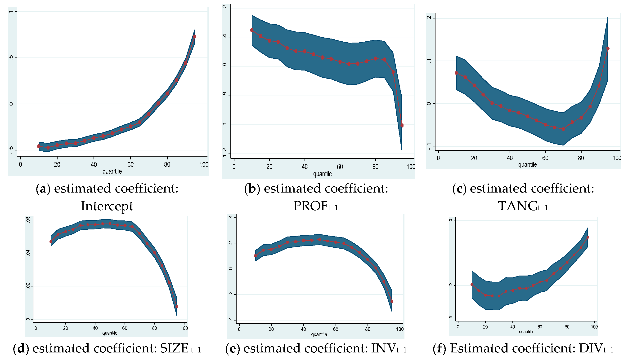
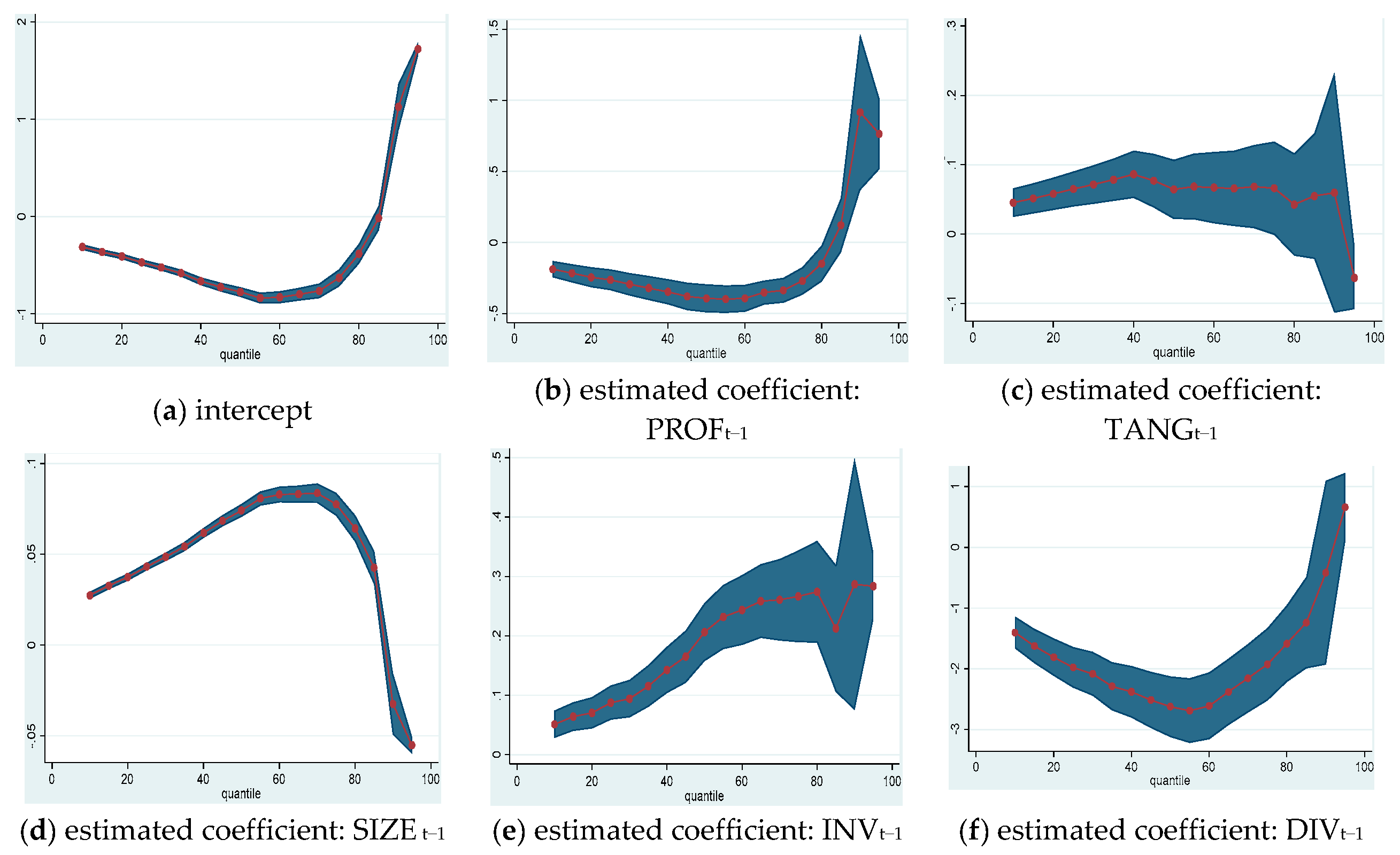
5.1. Main Findings

The main empirical results of the three models are presented in

Table 4. The results of the first model in all quantile levels.

Coefficient	Quantiles									Fixed Effect Regression
	10	20	30	40	50	60	70	80	90
Panel A: Book Leverage, all samples (14,806 observations)
βprof	−0.494 a	−0.593 a	−0.647 a	−0.655 a	−0.693 a	−0.708 a	−0.700 a	−0.639 a	−0.699 a	−0.748 a
	(0.026)	(0.025)	(0.024)	(0.023)	(0.022)	(0.023)	(0.022)	(0.021)	(0.024)	(0.016)
βtang	0.101 a	0.077 a	0.035 b	0.035	0.001	−0.021	−0.035b	−0.014	0.055 a	−0.037 b
	(0.021)	(0.020)	(0.019)	(0.018)	(0.018)	(0.018)	(0.018)	(0.016)	(0.018)	(0.021)
βsize	0.046 a	0.052 a	0.055 a	0.056 a	0.056 a	0.056 a	0.051 a	0.040 a	0.022 a	0.013 a
	(0.002)	(0.002)	(0.002)	(0.001)	(0.001)	(0.001)	(0.001)	(0.001)	(0.002)	(0.002)
βinv	0.099 a	0.149 a	0.203 a	0.218 a	0.225 a	0.205 a	0.166 a	0.069 a	−0.097 a	0.140 a
	(0.023)	(0.022)	(0.021)	(0.020)	(0.023)	(0.020)	(0.020)	(0.018)	(0.021)	(0.018)
β0	−0.464 a	−0.451 a	−0.430 a	−0.374 a	−0.322 a	−0.247 a	−0.109 a	0.110 a	0.443 a	0.322 a
	(0.025)	(0.023)	(0.022)	(0.021)	(0.021)	(0.021)	(0.021)	(0.020)	(0.022)	(0.025)
R2	0.0737	0.1016	0.1228	0.136	0.1444	0.1379	0.1246	0.1025	0.0718	0.14
Panel B: Market Leverage, all samples (14,806 Observations)
βprof	−0.293 a	−0.381 a	−0.450 a	−0.526 a	−0.591 a	−0.590 a	−0.499 a	−0.268 a	0.885 a	0.120 a
	(0.014)	(0.016)	(0.018)	(0.022)	(0.028)	(0.033)	(0.038)	(0.046)	(0.104)	(0.021)
βtang	0.066 a	0.085 a	0.102 a	0.122 a	0.103 a	0.106 a	0.100 a	0.066 b	0.066	−0.198 a
	(0.011)	(0.012)	(0.015)	(0.018)	(0.022)	(0.026)	(0.030)	(0.036)	(0.082)	(0.028)
βsize	0.026 a	0.036 a	0.047 a	0.060 a	0.073 a	0.081 a	0.082 a	0.063 a	−0.033 a	−0.019 a
	(0.012)	(0.001)	(0.001)	(0.001)	(0.002)	(0.002)	(0.002)	(0.003)	(0.007)	(0.002)
βinv	−0.317	0.068 a	0.092 a	0.140 a	0.203 a	0.240 a	0.258 a	0.272 a	0.286 a	0.412 a
	(0.013)	(0.014)	(0.016)	(0.020)	(0.024)	(0.029)	(0.033)	(0.040)	(0.091)	(0.024)
β0	−0.317 a	−0.414 a	−0.528 a	−0.669 a	−0.781 a	−0.836 a	−0.769 a	−0.387 a	1.126 a	0.618 a
	(0.013)	(0.015)	(0.017)	(0.021)	(0.026)	(0.031)	(0.035)	(0.043)	(0.098)	(0.032)
R2	0.0908	0.1205	0.1368	0.1445	0.1316	0.1147	0.0884	0.0371	0.0079	0.138

Standard deviation is in parentheses ( ); ^a significant at 0.01 level, ^b significant at 0.05 level.

,

Table 5. The results of the second model in all quantile levels.

Coefficient	Quantiles									Fixed Effect Regression
	10	20	30	40	50	60	70	80	90
Panel A: Book Leverage, all samples (14,806 observations)
βprof	−0.346 a	−0.420 a	−0.472 a	−0.493 a	−0.535 a	−0.565 a	−0.577 a	−0.542 a	−0.636 a	−0.750 a
	(0.027)	(0.026)	(0.025)	(0.023)	(0.023)	(0.023)	(0.023)	(0.022)	(0.025)	(0.016)
βtang	0.072 a	0.042 b	0.001	−0.016	−0.030 c	−0.049 a	−0.060 a	−0.033 b	0.042 b	−0.037 c
	(0.020)	(0.019)	(0.019)	(0.018)	(0.017)	(0.018)	(0.017)	(0.016)	(0.019)	(0.021)
βsize	0.047 a	0.053 a	0.057 a	0.057 a	0.058 a	0.057 a	0.052 a	0.071 a	0.022 a	0.013 a
	(0.002)	(0.002)	(0.002)	(0.001)	(0.001)	(0.001)	(0.001)	(0.018)	(0.002)	(0.002)
βinv	0.102 a	0.152 a	0.206 a	0.221 a	0.228 a	0.208 a	0.071 a	0.071 a	0.071 a	0.140 a
	(0.023)	(0.022)	(0.021)	(0.001)	(0.020)	(0.020)	(0.019)	(0.018)	(0.021)	(0.018)
βdiv	−1.962 a	−2.295 a	−2.321 a	−2.154 a	−2.089 a	−1.892 a	−1.629 a	−1.284 a	−0.840 a	0.047
	(0.115)	(0.109)	(0.104)	(0.098)	(0.097)	(0.098)	(0.098)	(0.092)	(0.104)	(0.076)
β0	−0.460 a	−0.446 a	−0.424 a	−0.368 a	−0.317 a	−0.242 a	−0.105 a	0.113 a	0.445 a	0.047
	(0.024)	(0.023)	(0.022)	(0.021)	(0.021)	(0.021)	(0.021)	(0.019)	(0.022)	(0.076)
R2	0.092	0.128	0.152	0.163	0.170	0.159	0.141	0.114	0.076	0.140
Panel B: Market Leverage, all samples (14,806 observations)
βprof	−0.187 a	−0.244 a	−0.293 a	−0.346 a	−0.393 a	−0.392 a	−0.336 a	−0.148 a	0.916 a	0.123 a
	(0.014)	(0.016)	(0.019)	(0.023)	(0.029)	(0.034)	(0.040)	(0.048)	(0.110)	(0.021)
βtang	0.045 a	0.058 a	0.071 a	0.086 a	0.064 a	0.067 b	0.068 b	0.042	0.060	−0.199 a
	(0.011)	(0.012)	(0.014)	(0.017)	(0.022)	(0.026)	(0.030)	(0.036)	(0.082)	(0.028)
βsize	0.027 a	0.037 a	0.049 a	0.062 a	0.074 a	0.083 a	0.084 a	0.064 a	−0.032 a	−0.019 a
	(0.012)	(0.001)	(0.001)	(0.001)	(0.002)	(0.002)	(0.002)	(0.003)	(0.007)	(0.002)
βinv	−1.404 a	0.070 a	0.094 a	0.143 a	0.206 a	0.261 a	0.261 a	0.274 a	0.287 a	0.412 a
	(0.059)	(0.013)	(0.016)	(0.019)	(0.024)	(0.029)	(0.033)	(0.040)	(0.091)	(0.024)
βdiv	−1.404 a	−1.811 a	−2.085 a	−2.381 a	−2.627 a	−2.613 a	−2.158 a	−1.588 a	−0.419	−0.091
	(0.059)	(0.068)	(0.080)	(0.097)	(0.120)	(0.144)	(0.166)	(0.203)	(0.460)	(0.098)
β0	−0.313 a	−0.410 a	−0.524 a	−0.664 a	−0.775 a	−0.829 a	−0.764 a	−0.383 a	1.127 a	0.616 a
	(0.013)	(0.014)	(0.017)	(0.021)	(0.026)	(0.030)	(0.035)	(0.043)	(0.098)	(0.032)
R2	0.12	0.16	0.17	0.18	0.16	0.13	0.10	0.04	0.01	0.03

Standard deviation is in parentheses ( ); ^a significant at 0.01 level, ^b significant at 0.05 level, ^c significant at 0.10 level.

and

Table 6. The results of the third model in all quantile levels.

Coefficient	Quantiles									Fixed Effect Regression
	10	20	30	40	50	60	70	80	90
Panel A: Book leverage, All samples (14,806 observations)
βblev	0.013 c	0.010 b	0.019 a	0.022 a	0.032 a	0.037 a	0.061 a	0.080 a	0.109 a	0.018 a
	(0.008)	(0.005)	(0.005)	(0.005)	(0.006)	(0.006)	(0.007)	(0.009)	(0.012)	(0.006)
βprof	0.244 a	0.135 a	0.123 a	0.123 a	0.108 a	0.092 a	0.102 a	0.100 a	0.134 a	0.035 a
	(0.018)	(0.012)	(0.012)	(0.013)	(0.013)	(0.015)	(0.018)	(0.022)	(0.029)	(0.011)
βsize	−0.003 a	−0.003 a	−0.005 a	−0.006 a	−0.006 a	−0.005 a	−0.007 a	−0.007 a	−0.007 a	−0.017 a
	(0.001)	(0.001)	(0.001)	(0.001)	(0.001)	(0.001)	(0.001)	(0.001)	(0.002)	(0.001)
βdiv	−0.115	−0.138 a	−0.161 a	−0.176 a	−0.255 a	−0.368 a	−0.480 a	−0.559 a	−0.624 a	−0.298 a
	(0.072)	(0.047)	(0.046)	(0.050)	(0.005)	(0.059)	(0.071)	(0.088)	(0.114)	(0.048)
β0	0.003	0.054 a	0.096 a	0.117 a	0.157 a	0.180 a	0.233 a	0.274 a	0.328 a	0.339 a
	(0.015)	(0.010)	(0.010)	(0.010)	(0.011)	(0.012)	(0.015)	(0.018)	(0.024)	(0.015)
R2 (%)	1.35	1.01	0.94	0.65	0.78	0.75	1.02	0.98	0.89	2.30
Panel B: Market leverage, all samples (14,806 observations)
βmlev	0.003	0.007 b	0.013 a	0.016 a	0.025 a	0.031 a	0.047 a	0.063 a	0.079 a	0.020 a
	(0.005)	(0.003)	(0.003)	(0.004)	(0.004)	(0.004)	(0.005)	(0.006)	(0.008)	(0.004)
βprof	0.231 a	0.124 a	0.103 a	0.082 a	0.073 a	0.050 a	0.035 b	0.011	0.015	0.014
	(0.017)	(0.011)	(0.011)	(0.012)	(0.013)	(0.014)	(0.017)	(0.021)	(0.027)	(0.010)
βsize	−0.003 c	−0.003 a	−0.004 a	−0.004 a	−0.005 a	−0.004 a	−0.006 a	−0.006 a	−0.004 a	−0.015 a
	(0.072)	(0.001)	(0.001)	(0.001)	(0.001)	(0.001)	(0.001)	(0.001)	(0.002)	(0.001)
βdiv	0.003 c	−0.137 a	−0.161 a	−0.172 a	−0.247 a	−0.355 a	−0.465 a	−0.539 a	−0.608 a	−0.292 a
	(0.015)	(0.047)	(0.046)	(0.050)	(0.053)	(0.059)	(0.071)	(0.088)	(0.114)	(0.047)
β0	0.003	0.053 a	0.095 a	0.116 a	0.155 a	0.177 a	0.229 a	0.268 a	0.321 a	0.321 a
	(0.015)	(0.010)	(0.010)	(0.010)	(0.011)	(0.012)	(0.015)	(0.018)	(0.024)	(0.016)
R2 (%)	1.30	1.00	0.90	0.70	0.80	0.90	1.10	1.10	1.00	2.50

Standard deviation is in parentheses ( ); ^a significant at 0.01 level, ^b significant at 0.05 level, ^c significant at 0.10 level.

and Figure A1, Figure A2, Figure A3, Figure A4, Figure A5 and Figure A6 (See Appendix A). In the first model, a firm with higher profitability had lower leverage. A firm with more tangible assets, a bigger size, and more investments had higher leverage. The results of firm size on leverage supported TOT, while the investment and profitability supported POT. In the second model, adding the dividend payout ratio variable, the significance and direction of profitability, tangible assets, firm size, and investment opportunities remained as in the first model. A firm with a higher dividend ratio also had lower leverage. This finding agreed with POT.

The significance of tangible assets was surprising. For the fixed effect regression, the negative effect of tangible assets on both books and the market was significant and consistent in the first and second models, thereby supporting POT. With quantile regression, the effect of tangible assets on book leverage changed from positive (supporting TOT) under low leverage to negative significance under high leverage (especially significant and consistent in the second model). For market leverage, the effect of tangible assets supports TOT.

In the third model, we found that firm size and dividend payout ratios were negatively related to investment opportunities, while leverage and profitability had a positive relationship. These results were consistent for book and market leverages. The overall results indicated that the financing decisions of Chinese manufacturing companies are explainable by pecking order theory.

5.2. Leverage and Profitability

TOT predicts that highly profitable firms often consider using debt to gain tax shield benefits. Fama and French (2002) noted that firms with strong profits can increase their debt. This is also true for firms with sufficient free cash flow (Jensen and Meckling [49]; Easterbrook [7]; Jensen [50]).

In contrast, POT argues that because firms prefer to use internal financing to fund their growth and to pay dividends if dividends and investments are fixed, the relationship between profitability and leverage is negative. Frank and Goyal [43] also suggested that profitability is often negatively correlated with leverage. This finding agrees with Kester [51] for US and Japanese manufacturing firms, Friend and Lang [52] for firms listed on the New York Stock Exchange, Wald [31] for the five most developed countries (including the USA), and Chen [11] for 88 Chinese firms during the period of 1995–2000.

We also found that the negative effect of profitability on book leverage strongly (and consistently more than market leverage in all quantiles) supported POT. However, for market leverage, the profitability significance became positive in the highest quantile, as did the fixed effect regression (in both the first and the second models). This implied that given high market leverage, Chinese manufacturing firms must consider the trade-off in following TOT when confronted with high debt and increasing financial distress costs.

This finding further supported the POT argument that highly profitable firms prefer to use internal financing rather than debt. POT assumes information asymmetry, and the first model results indicated that information asymmetry in the Chinese market was an important factor affecting the capital structure decisions for Chinese manufacturing companies. The profitability results supported the hypothesis that growth opportunities are also significant (with positive significance), thereby supporting POT.

The evidence showed that the effect of profit on the leverage of large Chinese firms was much stronger than that of small firms. We divided the sample into three groups according to firm size (smallest, medium, and biggest size), and the empirical results indicated that the impact of profit on leverage (both book and market) increased sharply (see

Table 7. The effect of profitability on leverage by firm size (the first model).

Coefficient	Quantiles									Fixed Effect Regression
	10	20	30	40	50	60	70	80	90
Panel A: Book Leverage
Smallest size (4471 observations)
βprof	−0.264 a	−0.331 a	−0.374 a	−0.402 a	−0.452 a	−0.477 a	−0.531 a	−0.638 a	−0.734 a	−0.647 a
	(0.029)	(0.033)	(0.034)	(0.034)	(0.036)	(0.036)	(0.037)	(0.042)	(0.047)	(0.024)
Medium size (4895 observations)
βprof	−0.525 a	−0.544 a	−0.566 a	−0.560 a	−0.572 a	−0.620 a	−0.658 a	−0.659 a	−0.818 a	−1.039 a
	(0.046)	(0.039)	(0.037)	(0.036)	(0.037)	(0.039)	(0.040)	(0.041)	(0.049)	(0.034)
Biggest size (5440 observations)
βprof	−1.248 a	−1.212 a	−1.179 a	−1.063 a	−1.017 a	−0.897 a	−0.772 a	−0.682 a	−0.744 a	−0.502 a
	(0.062)	(0.052)	(0.046)	(0.043)	(0.040)	(0.036)	(0.033)	(0.033)	(0.041)	(0.025)
Panel B: Market Leverage
Smallest size (4471 observations)
βprof	−0.118 a	−0.153 a	−0.173 a	−0.180 a	−0.202 a	−0.243 a	−0.245 a	−0.182 a	4.777 a	0.244 a
	(0.013)	(0.015)	(0.017)	(0.020)	(0.024)	(0.032)	(0.050)	(0.078)	(0.465)	(0.035)
Medium size (4895 observations)
βprof	−0.118 a	−0.153 a	−0.173 a	−0.180 a	−0.202 a	−0.243 a	−0.245 a	−0.182 a	4.777 a	0.244 a
	(0.013)	(0.015)	(0.017)	(0.020)	(0.024)	(0.032)	(0.050)	(0.078)	(0.465)	(0.035)
Panel C: Biggest size (5440 observations)
βprof	−1.120 a	−1.276 a	−1.354 a	−1.357 a	−1.172 a	−1.035 a	−0.845 a	−0.674 a	−0.119 a	−0.308 a
	(0.044)	(0.049)	(0.055)	(0.058)	(0.060)	(0.062)	(0.064)	(0.075)	(0.135)	(0.038)

Standard deviation is in parentheses ( ); ^a significant at 0.01 level.

and

Table 8. The effect of profitability on leverage by firm size (the second model).

Coefficient	Quantiles									Fixed Effect Regression
	10	20	30	40	50	60	70	80	90
Panel A: Book Leverage
Smallest size (4471 observations)
βprof	−0.198 a	−0.247 a	−0.287 a	−0.304 a	−0.360 a	−0.387 a	−0.437 a	−0.550 a	−0.669 a	−0.650 a
	(0.030)	(0.033)	(0.035)	(0.035)	(0.036)	(0.036)	(0.038)	(0.043)	(0.049)	(0.024)
Medium size (4895 observations)
βprof	−0.364 a	−0.397 a	−0.434 a	−0.427 a	−0.443 a	−0.499 a	−0.538 a	−0.557 a	−0.744 a	−1.045 a
	(0.047)	(0.041)	(0.038)	(0.037)	(0.038)	(0.040)	(0.042)	(0.043)	(0.051)	(0.035)
Biggest size (5440 observations)
βprof	−0.882 a	−0.881 a	−0.889 a	−0.813 a	−0.797 a	−0.722 a	−0.629 a	−0.578 a	−0.671 a	−0.466 a
	(0.068)	(0.058)	(0.051)	(0.047)	(0.044)	(0.040)	(0.036)	(0.036)	(0.045)	(0.025)
Panel B: Market Leverage
Smallest size (4471 observations)
βprof	−0.081 a	−0.105 a	−0.121 a	−0.120 a	−0.139 a	−0.174 a	−0.166 a	−0.128 a	4.431 a	0.233 a
	(0.013)	(0.015)	(0.017)	(0.020)	(0.024)	(0.032)	(0.051)	(0.080)	(0.479)	(0.035)
Medium size (4895 observations)
βprof	−0.081 a	−0.105 a	−0.121 a	−0.120 a	−0.139 a	−0.174 a	−0.166 a	−0.128 a	4.431 a	0.157 a
	(0.013)	(0.015)	(0.017)	(0.020)	(0.024)	(0.032)	(0.051)	(0.080)	(0.479)	(0.038)
Panel C: Biggest size (5440 observations)
βprof	−0.711 a	−0.862 a	−0.901 a	−0.921 a	−0.773 a	−0.682 a	−0.541 a	−0.381 a	0.178 a	−0.211 a
	(0.047)	(0.053)	(0.060)	(0.064)	(0.066)	(0.069)	(0.071)	(0.084)	(0.151)	(0.039)

Standard deviation is in parentheses ( ); ^a significant at 0.01 level.

). At least for large firms, this strongly supported POT. This result also suggested that the ability of Chinese manufacturing firms to borrow was affected by the scale or threat of bankruptcy costs (especially for small, high-debt firms).

This finding agrees with Chen and Strange [53], who used a sample of 972 Chinese companies listed on the Shanghai and Shenzhen Stock Exchange in 2003, but disagrees with Chen [11], who studied 88 Chinese companies during the period of 1995–2000.

5.3. Leverage and Firm Size

TOT predicts that the debt capacity of large companies will be higher than that of small companies. However, big firms often have more diversified fields of business than small ones, thereby facing lower bankruptcy costs and easier access to low-risk debt securities. Furthermore, bigger firms usually have more tangible assets, thus demonstrating their ability to repay loans better than small firms.

Meanwhile, according to POT, because of the information asymmetry between “inside” and “outside”, firms prefer to use internal capital over debt securities. However, Kester [51] argued that big firms listed on capital markets often have less information asymmetry than small ones, so they can access the debt or equity markets with a lower cost than small companies.

Chen [11] noted that there is still much debate about the relationship between leverage and firm size. Kadapakkam et al. [54] argued that small firms are often more affected by internal finance than large firms because small firms have less access to capital markets.

Marsh [55] found that small firms prioritize short-term debt, while long-term debt is prioritized by large firms. Meanwhile, Rajan and Zingales [22] and Wald [31] proposed a positive relationship between debt and firm size in most developed countries (except Germany). Chen [11] found that, although total debt has a positive relationship with firm size, overall long-term debt negatively affects size. Titman and Wessels [56] and Mazur [57] also found evidence to support the hypothesis of a negative relationship between size and leverage.

5.4. Leverage and Investment Opportunities

Frank and Goyal [43] argued that higher growth opportunities increase the cost of financial distress and debt-related agency problems and reduce cash flow problems. High-growth firms also place greater value on investing. Hence, TOT predicts that investment opportunities reduce a firm’s leverage. In contrast, POT suggests that firms investing more and holding their profitability fixed will accumulate more debt over time. The results from Models 1 and 3 supported this argument.

5.5. Leverage and Dividend Payout Ratio

Myers and Majluf [3] found that firms prefer to use internal finances, rather than issue debt and equity, although POT cannot directly explain why firms pay or do not pay dividends. However, if a firm chooses to pay a dividend, this choice decreases its internal financing, so POT will affect a firm’s decision to pay dividends. Firms with good investments or growth opportunities will carefully consider dividend payouts (one way of signaling to investors that the firm has good business). Firms with good profitability, ceteris paribus, can pay more dividends than firms with low profit. According to TOT, there is no prediction about market leverage because if profitability increases so does market value. Reading [58] argued that big firms are preferred by large investors because they save transaction costs and that, statistically and economically, big firms prefer to pay dividends more than smaller ones.

We found that both book and market leverage were negatively related to the dividend payout ratio. This finding was consistent with the argument of POT. Fama and French [23] argued that in the POT world, firms paying higher dividends have less leverage. Furthermore, the changes in both short-term profitability and investment opportunities are also permeated by the volatility of debt. In the second model, we found that the dividend payout ratio yielded the strongest effect on both book and market leverage. By analyzing the performance of some USA companies, Baskin [5] concluded that, based on the Lintner model, past dividends affect current dividends directly. The results from the second model in our paper were not consistent with those obtained from Baskin [5] and Allen [4], who tested POT by examining Australian companies, and Tong and Green [8], who tested the theory by using Chinese firms. In addition, our results were also not consistent with those of Reading [58], who argued that bigger firms prefer to pay dividends more than small firms.

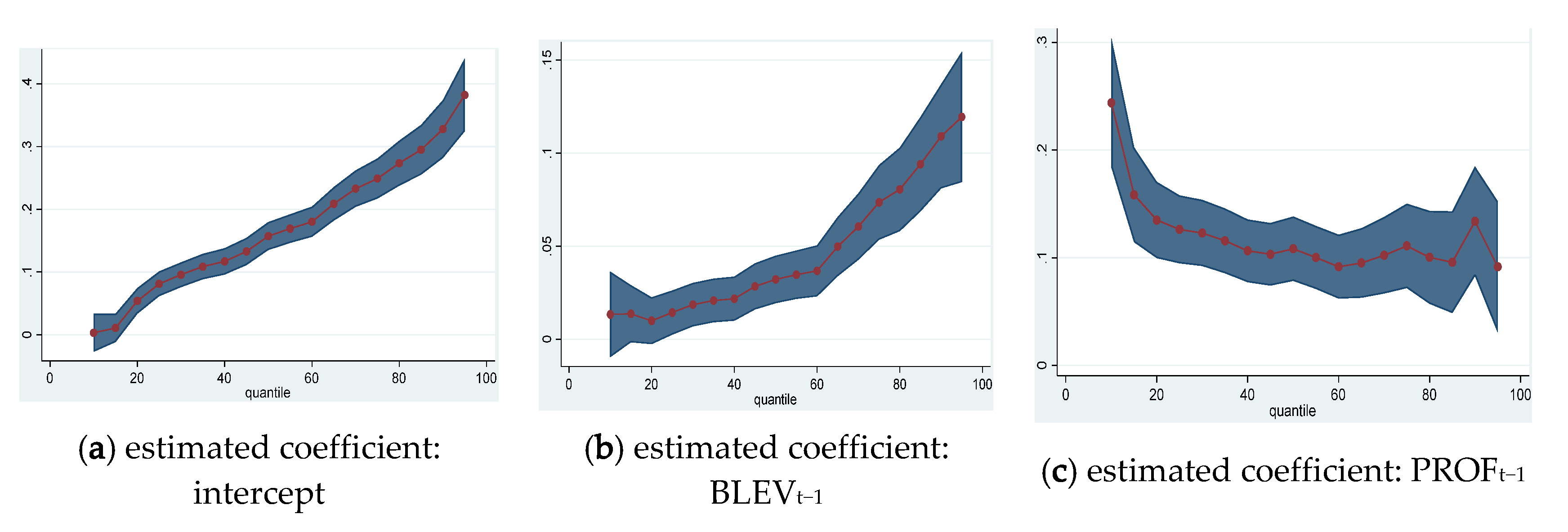
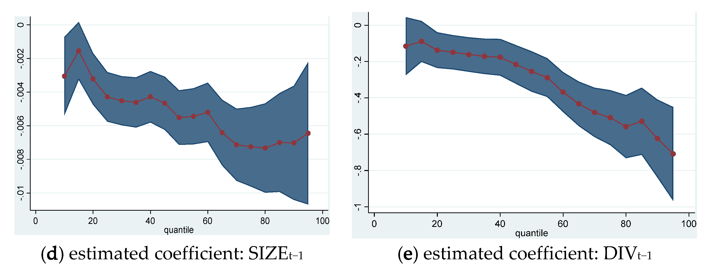
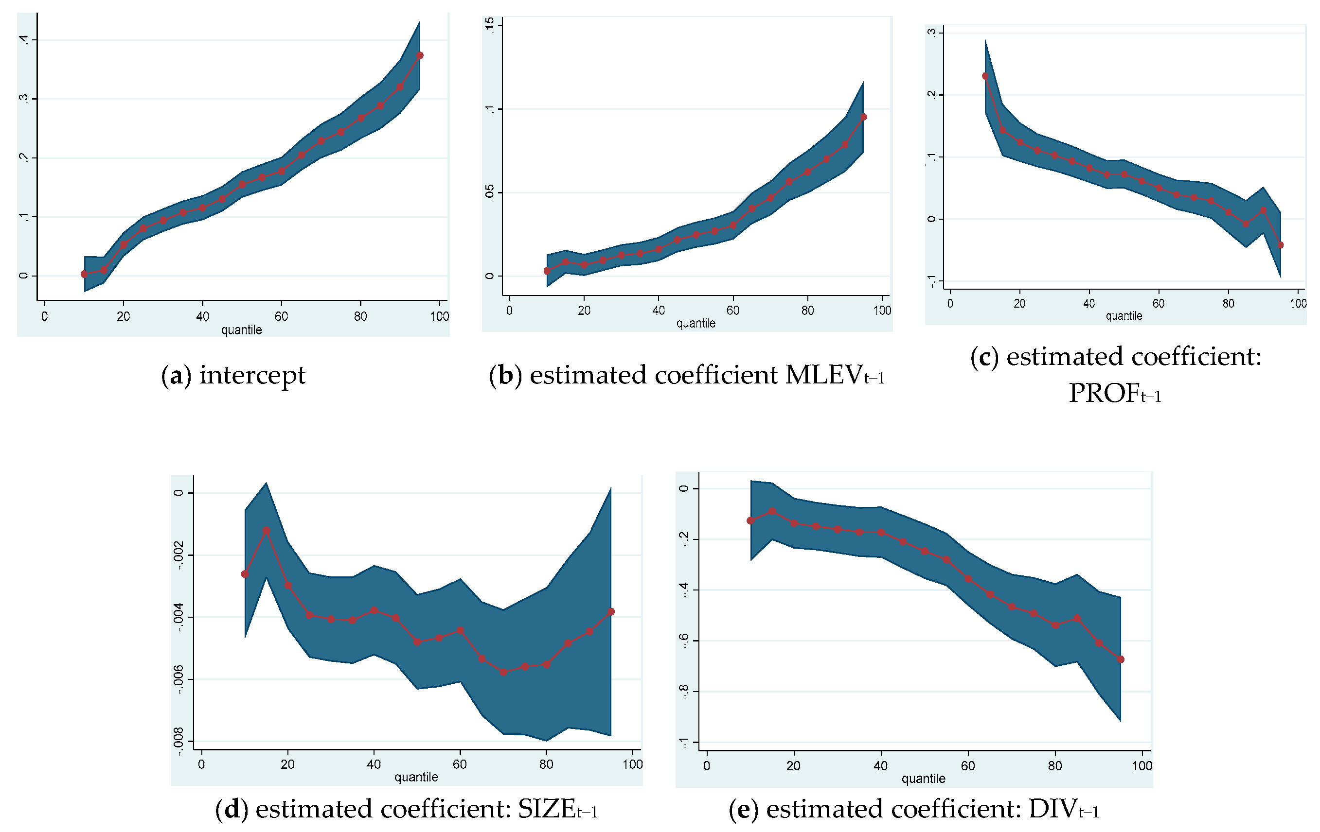
5.6. Investment Opportunities and Dividend Payout Ratio

Dividends signal potential growth and that a firm has sufficient internal financial resources to ensure they can both pay dividends and continue to invest in the future. Firms with large and increasing dividends also demonstrate sustainability and growth potential. According to Fama and French [23], based on POT, firms paying a dividend will decrease their investments and leverage. According to Baskin [5], because of dividend payments, firms have a reduced capacity for internal financing, which may reduce their ability to invest. Thus, if a firm wants to invest more, it must obtain external funds. This argument agrees with Fama and French [23], who argued that, given constant profitability, firms that pursue more investments will have more leverage. Our results (shown in Table 6) also demonstrated that the dividend payout ratio has negative significance for investment opportunities and that the impact of the dividend payout ratio increases from low to high quantile levels.

Model 3 explores the relationship between investment opportunities and leverage and the dividend payout ratio among other independent variables (Table 6). The results indicated that firms with higher profitability invested more than firms with lower profitability and that dividends also had a negative effect on investment.

5.7. Robustness Checks

We divided the sample into three groups according to firm size (smallest, medium, and biggest size), the empirical results indicated that the impact of profitability on leverage increases sharply from the smallest size to biggest size (Table 7 and Table 8). This led to the conclusion that the effect of profit on the leverage of large Chinese firms was much stronger than that of small firms. In addition, the coefficient of fixed assets moved from positive (with smallest and medium size) to negative for the biggest size (for book leverage, see

Table 9. The effect of tangible assets on book leverage by firm size.

Coefficient	Quantiles									Fixed Effect Regression
	10	20	30	40	50	60	70	80	90
Panel A: The first model
Smallest size (4471 observations)
βtang	−0.016	0.066 c	0.109 a	0.071 c	0.077 b	0.120 a	0.198 a	0.262 a	0.374 a	0.275 a
	(0.031)	(0.035)	(0.036)	(0.037)	(0.038)	(0.038)	(0.040)	(0.045)	(0.051)	(0.041)
Medium size (4,895 observations)
βtang	0.148 a	0.068 a	0.041	0.021	−0.004	−0.032	−0.029	−0.012	0.057	−0.147 a
	(0.035)	(0.031)	(0.028)	(0.028)	(0.028)	(0.029)	(0.031)	(0.032)	(0.038)	(0.043)
Biggest size (5440 observations)
βtang	−0.009	−0.099 a	−0.158 a	−0.166 a	−0.180 a	−0.151 a	−0.125 a	−0.099 a	−0.039 c	−0.173 a
	(0.035)	(0.029)	(0.026)	(0.024)	(0.022)	(0.020)	(0.018)	(0.018)	(0.023)	(0.025)
Panel B: The second model
Smallest size (4471 observations)
βtang	−0.034	0.440	0.085 b	0.044	0.052	0.096 b	0.173 a	0.238 a	0.357 a	0.277 a
	(0.031)	(0.035)	(0.036)	(0.036)	(0.038)	(0.038)	(0.039)	(0.045)	(0.051)	(0.041)
Medium size (4895 observations)
βtang	0.116 a	0.040	0.015	−0.005	−0.029	−0.055 c	−0.052 c	−0.032	0.043	−0.146 b
	(0.035)	(0.030)	(0.028)	(0.027)	(0.028)	(0.029)	(0.031)	(0.032)	(0.038)	(0.043)
Biggest size (5440 observations)
βtang	−0.044	−0.131 a	−0.185 a	−0.191 a	−0.201 a	−0.168 a	−0.139 a	−0.106 a	−0.046 b	−0.178 a
	(0.034)	(0.029)	(0.025)	(0.023)	(0.022)	(0.020)	(0.018)	(0.018)	(0.023)	(0.025)

Standard deviation is in parentheses ( ); ^a significant at 0.01 level, ^b significant at 0.05 level, ^c significant at 0.10 level.

). This finding supported the notion that large firms more strongly follow POT than small and medium ones. This also suggested that the ability of Chinese manufacturing firms to borrow was affected by the scale or threat of bankruptcy costs (especially for small, high debt firms).

The effect of dividends on leverage in the first and the second models showed that the negative effect of dividends on both book and market leverage was stronger for the biggest firms than for those of a medium and small size (

Table 10. The effect of dividend on leverage by firm size (the second model).

Coefficient	Quantiles									Fixed Effect Regression
	10	20	30	40	50	60	70	80	90
Panel A: Book Leverage
Smallest size (4471 observations)
βdiv	−1.253 a	−1.586 a	−1.656 a	−1.849 a	−1.739 a	−1.700 a	−1.774 a	−1.662 a	−1.226 a	0.135
	(0.136)	(0.153)	(0.161)	(0.162)	(0.167)	(0.167)	(0.175)	(0.197)	(0.224)	(0.126)
Medium size (4895 observations)
βprof	−2.192 a	−1.998 a	−1.804 a	−1.812 a	−1.574 a	−1.652 a	−1.637 a	−1.397 a	−1.009 a	0.171
	(0.196)	(0.169)	(0.158)	(0.155)	(0.158)	(0.166)	(0.174)	(0.178)	(0.212)	(0.158)
Biggest size (5440 observations)
βprof	−2.913 a	−2.637 a	−2.301 a	−1.994 a	−1.751 a	−1.389 a	−1.137 a	−0.823 a	−0.582 a	−0.492 a
	(0.249)	(0.211)	(0.186)	(0.172)	(0.162)	(0.146)	(0.133)	(0.029)	(0.036)	(0.100)
Panel B: Market Leverage
Smallest size (4471 observations)
βprof	−0.702 a	−0.917 a	−0.986 a	−1.137 a	−1.181 a	−1.291 a	−1.494 a	−1.019 a	6.547 a	0.532 a
	(0.061)	(0.068)	(0.078)	(0.092)	(0.112)	(0.149)	(0.235)	(0.371)	(2.212)	(0.179)
Medium size (4895 observations)
βprof	−1.587 a	−1.674 a	−1.863 a	−2.098 a	−2.139 a	−2.131 a	−1.746 a	−1.198 a	0.766	−0.009
	(0.102)	(0.112)	(0.124)	(0.143)	(0.168)	(0.206)	(0.232)	(0.304)	(0.581)	(0.170)
Panel C: Biggest size (5440 observations)
βprof	−3.252 a	−3.292 a	−3.608 a	−3.466 a	−3.177 a	−2.184 a	−2.424 a	−2.337 a	−2.373 a	−1.337 a
	(0.174)	(0.193)	(0.218)	(0.233)	(0.240)	(0.251)	(0.259)	(0.305)	(0.550)	(0.153)

Standard deviation is in parentheses ( ); ^a significant at 0.01 level.

). This finding strongly supports the argument of Fama and French [23] and POT.

Furthermore, we examined each model’s robustness by equal testing among the different quantile levels.

Table 11. Robust tests of the equality of slope estimates across various quantiles.

Quantiles	F-Statistic (p Value)
	The First Model	The Second Model	The Third Model
0.1 versus 0.2	chi2 (4) = 36.98 Prob > chi2 = 0.0000	chi2 (5) = 48.88 Prob > chi2 = 0.0000	chi2 (4) = 82.13 Prob > chi2 = 0.0000
0.2 versus 0.3	chi2 (4) = 25.40 Prob > chi2 = 0.0000	chi2 (5) = 25.51 Prob > chi2 = 0.0001	chi2 (4) = 21.41 Prob > chi2 = 0.0003
0.3 versus 0.4	chi2 (4) = 2.70 Prob > chi2 = 0.6087	chi2 (5) = 8.48 Prob > chi2 = 0.1316	chi2 (4) = 17.36 Prob > chi2 = 0.0016
0.4 versus 0.5	chi2 (4) = 7.56 Prob > chi2 = 0.1092	chi2 (5) = 8.55 Prob > chi2 = 0.1282	chi2 (4) = 30.43 Prob > chi2 = 0.0000
0.5 versus 0.6	chi2 (4) = 19.00 Prob > chi2 = 0.0008	chi2 (5) = 28.29 Prob > chi2 = 0.0000	chi2 (4) = 37.44 Prob > chi2 = 0.0000
0.6 versus 0.7	chi2 (4) = 48.60 Prob > chi2 = 0.0000	chi2 (5) = 64.15 Prob > chi2 = 0.0000	chi2 (4) = 44.84 Prob > chi2 = 0.0000
0.7 versus 0.8	chi2 (4) = 173.84 Prob > chi2 = 0.0000	chi2 (5) = 198.82 Prob > chi2 = 0.0000	chi2 (4) = 23.53 Prob > chi2 = 0.0001
0.8 versus 0.9	chi2 (4) = 320.66 Prob > chi2 = 0.0000	chi2 (5) = 349.57 Prob > chi2 = 0.0000	chi2 (4) = 11.53 Prob > chi2 = 0.0212

and

Table 12. Robust tests of the equality of slope estimates across various quantiles.

Quantiles	The First Model	The Second Model	The Third Model
0.1 versus 0.2	chi2 (4) = 201.79 Prob > chi2 = 0.0000	chi2 (5) = 254.70 Prob > chi2 = 0.0000	chi2 (4) = 82.43 Prob > chi2 = 0.0000
0.2 versus 0.3	chi2 (4) = 220.87 Prob > chi2 = 0.0000	chi2 (5) = 244.66 Prob > chi2 = 0.0000	chi2 (4) = 23.25 Prob > chi2 = 0.0001
0.3 versus 0.4	chi2 (4) = 256.90 Prob > chi2 = 0.0000	chi2 (5) = 279.11 Prob > chi2 = 0.0000	chi2 (4) = 11.24 Prob > chi2 = 0.0240
0.4 versus 0.5	chi2 (4) = 142.25 Prob > chi2 = 0.0000	chi2 (5) = 153.02 Prob > chi2 = 0.0000	chi2 (4) = 27.00 Prob > chi2 = 0.0000
0.5 versus 0.6	chi2 (4) = 52.72 Prob > chi2 = 0.0000	chi2 (5) = 52.74 Prob > chi2 = 0.0000	chi2 (4) = 29.78 Prob > chi2 = 0.0000
0.6 versus 0.7	chi2 (4) = 17.38 Prob > chi2 = 0.0016	chi2 (5) = 36.14 Prob > chi2 = 0.0000	chi2 (4) = 48.57 Prob > chi2 = 0.0000
0.7 versus 0.8	chi2 (4) = 155.26 Prob > chi2 = 0.0000	chi2 (5) = 173.58 Prob > chi2 = 0.0000	chi2 (4) = 19.23 Prob > chi2 = 0.0007
0.8 versus 0.9	chi2 (4) = 527.63 Prob > chi2 = 0.0000	chi2 (5) = 539.02 Prob > chi2 = 0.0000	chi2 (4) = 12.45 Prob > chi2 = 0.0143

present the F-tests and p values for each pair of quantile levels (0.1–0.2, 0.2–0.3, …, 0.8–0.9). Most robustness tests rejected the null hypothesis at a 99% confidence level (i.e., that the coefficients of each quantile level are equal or homogeneous). These results confirmed that each model’s explanatory variables had different and significant effects on the dependent variables.

6. Conclusions

This study examines the sustainability of both POT and TOT in Chinese manufacturing firms for capital structure decisions by using panel data from 2011 to 2018. We applied three conditional quantile regression models to investigate the impact of the independent variables on the dependent variable at each quantile and determined the marginal effect of the independent variable on the dependent variable at each quantile.

From our first two models, we conclude that firms with a bigger size and more investments will lead to higher leverage, more profitable firms will require less leverage, and adding the dividend variable to the model will yield a strong and significant negative relationship between dividends and leverage. Our second model also concludes that dividends have the strongest negative impacts on both book and market leverage.

For fixed effect regressions, the negative impacts of tangible assets on both the book and market are significant and consistent, thus supporting POT. However, the signs of tangible assets lack consistency with the quantile regression results for both the first and second models. The impact of tangible assets on book leverage varies from positive (TOT support) under low leverage to negative significance under high leverage (especially in the second model). For market leverage, the effect of tangible assets supports TOT.

Our third model suggests that dividends and firm size have a negative relationship with investment. However, a firm that is more profitable and has higher leverage will invest more. Moreover, our third model suggests that the dividend payout ratio has the strongest negative impact on investment opportunities and that this impact increases from low quantile to high quantile levels. This finding suggests that, although dividends are a sign of future sustainable growth potential, paying dividends significantly reduces a firm’s investment opportunities.

Overall, the results of our paper indicate that the current financial decisions of Chinese listed firms in the manufacturing sector can be best explained by pecking order theory.

Our study investigated the Chinese manufacturing firms listed on both the Shanghai and the Shenzhen Stock Exchanges following the pecking order or trade-off theories in their capital structure choices. We did not focus on firms’ financial and risk management policies, which have been analyzed in recent research (Chen et al. [53] Chen et al. [59]; Potì et al. [60]). Moreover, although the Chinese manufacturing sector plays a leading role in the Chinese economy, it is not representative of the whole economy. Future studies should research other sectors or investigate differences in the capital structures of other important Chinese industries. In addition, scholars could investigate the consistency of our empirical findings with cash holding policies or the role of cash holdings in firms’ financial and risk management policies.

References

1. Modigliani, F.; Miller, M.H. The cost of capital, corporation finance and the theory of investment. American 1958, 1, 3. [Google Scholar]
2. Modigliani, F.; Miller, M.H. Corporate income taxes and the cost of capital: A correction. Am. Econ. Rev. 1963, 53, 433–443. [Google Scholar]
3. Myers, S.C.; Majluf, N.S. Corporate financing and investment decisions when firms have information that investors do not have. J. Financ. Econ. 1984, 13, 187–221. [Google Scholar] [CrossRef] [Green Version]
4. Allen, D.E. The pecking order hypothesis: Australian evidence. Appl. Financ. Econ. 1993, 3, 101–112. [Google Scholar] [CrossRef]
5. Baskin, J. An empirical investigation of the pecking order hypothesis. Financ. Manag. 1989, 26–35. [Google Scholar] [CrossRef]
6. De Jong, A.; Verbeek, M.; Verwijmeren, P. The impact of financing surpluses and large financing deficits on tests of the pecking order theory. Financ. Manag. 2010, 39, 733–756. [Google Scholar] [CrossRef]
7. Easterbrook, F.H. Two agency-cost explanations of dividends. Am. Econ. Rev. 1984, 74, 650–659. [Google Scholar]
8. Tong, G.; Green, C.J. Pecking order or trade-off hypothesis? Evidence on the capital structure of Chinese companies. Appl. Econ. 2005, 37, 2179–2189. [Google Scholar] [CrossRef]
9. Booth, L.; Aivazian, V.; Demirguc-Kunt, A.; Maksimovic, V. Capital structures in developing countries. J. Financ. 2001, 56, 87–130. [Google Scholar] [CrossRef]
10. De Jong, A.; Kabir, R.; Nguyen, T.T. Capital structure around the world: The roles of firm-and country-specific determinants. J. Bank. Financ. 2008, 32, 1954–1969. [Google Scholar] [CrossRef] [Green Version]
11. Chen, J.J. Determinants of capital structure of Chinese-listed companies. J. Bus. Res. 2004, 57, 1341–1351. [Google Scholar] [CrossRef]
12. Huang, G. The determinants of capital structure: Evidence from China. China Econ. Rev. 2006, 17, 14–36. [Google Scholar] [CrossRef]
13. Ni, J.; Yu, M. Testing the pecking-order theory: Evidence from Chinese listed companies. Chin. Econ. 2008, 41, 97–113. [Google Scholar] [CrossRef]
14. Li, K.; Yue, H.; Zhao, L. Ownership, institutions, and capital structure: Evidence from China. J. Comp. Econ. 2009, 37, 471–490. [Google Scholar] [CrossRef]
15. Tse, C.-B.; Rodgers, T. The capital structure of Chinese listed firms: Is manufacturing industry special? Manag. Financ. 2014, 40, 469–486. [Google Scholar] [CrossRef]
16. Zhou, T.; Xie, J. Ultimate ownership and adjustment speed toward target capital structures: Evidence from China. Emerg. Mark. Financ. Trade 2016, 52, 1956–1965. [Google Scholar] [CrossRef]
17. Ferrarini, B.; Hinojales, M.; Scaramozzino, P. Leverage and capital structure determinants of Chinese listed companies. In Asian Development Bank Economics Working Paper Series (509); Asian Development Bank: Mandaluyong City, Philippines, 2017. [Google Scholar]
18. Fattouh, B.; Scaramozzino, P.; Harris, L. Capital structure in South Korea: A quantile regression approach. J. Dev. Econ. 2005, 76, 231–250. [Google Scholar] [CrossRef] [Green Version]
19. Sánchez-Vidal, F.J. High debt companies’ leverage determinants in Spain: A quantile regression approach. Econ. Model. 2014, 36, 455–465. [Google Scholar] [CrossRef]
20. Sheikh, N.A.; Wang, Z. Determinants of capital structure. Manag. Financ. 2011, 37, 117–133. [Google Scholar]
21. Liu, W.-C.; Hsu, C.-M. Financial structure, corporate finance and growth of Taiwan’s manufacturing firms. Rev. Pacif. Basin Financ. Mark. Policies 2006, 9, 67–95. [Google Scholar] [CrossRef]
22. Rajan, R.G.; Zingales, L. What do we know about capital structure? Some evidence from international data. J. Financ. 1995, 50, 1421–1460. [Google Scholar] [CrossRef]
23. Fama, E.F.; French, K.R. Testing trade-off and pecking order predictions about dividends and debt. Rev. Financ. Stud. 2002, 15, 1–33. [Google Scholar] [CrossRef]
24. Shyam-Sunder, L.; Myers, S.C. Testing static tradeoff against pecking order models of capital structure. J. Financ. Econ. 1999, 51, 219–244. [Google Scholar] [CrossRef]
25. Frank, M.Z.; Goyal, V.K. The effect of market conditions on capital structure adjustment. Financ. Res. Lett. 2004, 1, 47–55. [Google Scholar] [CrossRef]
26. Frank, M.Z.; Goyal, V.K. Trade-off and pecking order theories of debt. In Handbook of Empirical Corporate Finance; Elsevier: Amsterdam, The Netherlands, 2008; pp. 135–202. [Google Scholar]
27. Chirinko, R.S.; Singha, A.R. Testing static tradeoff against pecking order models of capital structure: A critical comment. J. Financ. Econ. 2000, 58, 417–425. [Google Scholar] [CrossRef]
28. Frank, M.Z.; Goyal, V.K. Testing the pecking order theory of capital structure. J. Financ. Econ. 2003, 67, 217–248. [Google Scholar] [CrossRef] [Green Version]
29. Fama, E.F.; French, K.R. Financing decisions: Who issues stock? J. Financ. Econ. 2005, 76, 549–582. [Google Scholar] [CrossRef]
30. Hodder, J.E.; Senbet, L.W. International capital structure equilibrium. J. Financ. 1990, 45, 1495–1516. [Google Scholar] [CrossRef]
31. Wald, J.K. How firm characteristics affect capital structure: An international comparison. J. Financ. Res. 1999, 22, 161–187. [Google Scholar] [CrossRef]
32. Ozkan, A. Determinants of capital structure and adjustment to long run target: Evidence from UK company panel data. J. Bus. Financ. Account. 2001, 28, 175–198. [Google Scholar] [CrossRef]
33. Chui, A.C.; Lloyd, A.E.; Kwok, C.C. The determination of capital structure: Is national culture a missing piece to the puzzle? J. Int. Bus. Stud. 2002, 33, 99–127. [Google Scholar] [CrossRef]
34. Bevan, A.A.; Danbolt, J. Capital structure and its determinants in the UK-a decompositional analysis. Appl. Financ. Econ. 2002, 12, 159–170. [Google Scholar] [CrossRef] [Green Version]
35. Psillaki, M.; Daskalakis, N. Are the determinants of capital structure country or firm specific? Small Bus. Econ. 2009, 33, 319–333. [Google Scholar] [CrossRef]
36. Črnigoj, M.; Mramor, D. Determinants of capital structure in emerging European economies: Evidence from Slovenian firms. Emerg. Mark. Financ. Trade 2009, 45, 72–89. [Google Scholar] [CrossRef]
37. Al-Najjar, B.; Hussainey, K. Revisiting the capital-structure puzzle: UK evidence. J. Risk Financ. 2011, 12, 329–338. [Google Scholar] [CrossRef]
38. Graham, J.R.; Harvey, C.R. The theory and practice of corporate finance: Evidence from the field. J. Financ. Econ. 2001, 60, 187–243. [Google Scholar] [CrossRef]
39. Flannery, M.J.; Rangan, K.P. Partial adjustment toward target capital structures. J. Financ. Econ. 2006, 79, 469–506. [Google Scholar] [CrossRef]
40. Byoun, S. How and when do firms adjust their capital structures toward targets? J. Financ. 2008, 63, 3069–3096. [Google Scholar] [CrossRef]
41. Lemmon, M.L.; Roberts, M.R.; Zender, J.F. Back to the beginning: Persistence and the cross-section of corporate capital structure. J. Financ. 2008, 63, 1575–1608. [Google Scholar] [CrossRef]
42. Huang, R.; Ritter, J.R. Testing theories of capital structure and estimating the speed of adjustment. J. Financ. Quant. Anal. 2009, 44, 237–271. [Google Scholar] [CrossRef] [Green Version]
43. Frank, M.Z.; Goyal, V.K.J.F.M. Capital structure decisions: Which factors are reliably important? Financ. Manag. 2009, 38, 1–37. [Google Scholar] [CrossRef] [Green Version]
44. Chen, D.-H.; Chen, C.-D.; Chen, J.; Huang, Y.-F. Panel data analyses of the pecking order theory and the market timing theory of capital structure in Taiwan. Int. Rev. Econ. Financ. 2013, 27, 1–13. [Google Scholar] [CrossRef]
45. Qian, Y.; Tian, Y.; Wirjanto, T.S. Do Chinese publicly listed companies adjust their capital structure toward a target level? China Econ. Rev. 2009, 20, 662–676. [Google Scholar] [CrossRef]
46. Koenker, R.; Bassett, G., Jr. Regression quantiles. Econometrica 1978, 50, 33–50. [Google Scholar] [CrossRef]
47. Horowitz, J.L.; Lee, S. Nonparametric estimation of an additive quantile regression model. J. Am. Stat. Assoc. 2005, 100, 1238–1249. [Google Scholar] [CrossRef] [Green Version]
48. Koenker, R.; Hallock, K.F. Quantile regression. J. Econ. Perspect. 2001, 15, 143–156. [Google Scholar] [CrossRef]
49. Jensen, M.C.; Meckling, W.H. Agency Costs and the Theory of the Firm. J. Financ. Econ. 1976, 3, 305–360. [Google Scholar] [CrossRef]
50. Jensen, M.C. Agency costs of free cash flow, corporate finance, and takeovers. Am. Econ. Rev. 1986, 76, 323–329. [Google Scholar]
51. Kester, W.C. Capital and ownership structure: A comparison of United States and Japanese manufacturing corporations. Financ. Manag. 1986, 15, 5–16. [Google Scholar] [CrossRef]
52. Friend, I.; Lang, L.H. An empirical test of the impact of managerial self-interest on corporate capital structure. J. Financ. 1988, 43, 271–281. [Google Scholar] [CrossRef]
53. Chen, J.; Strange, R. The determinants of capital structure: Evidence from Chinese listed companies. Econ. Chang. Restruct. 2005, 38, 11–35. [Google Scholar] [CrossRef]
54. Kadapakkam, P.R.; Kumar, P.C.; Riddick, L.A. The impact of cash flows and firm size on investment: The international evidence. J. Bank. Financ. 1998, 22, 293–320. [Google Scholar] [CrossRef]
55. Marsh, P. The choice between equity and debt: An empirical study. J. Financ. 1982, 37, 121–144. [Google Scholar] [CrossRef]
56. Titman, S.; Wessels, R. The determinants of capital structure choice. J. Financ. 1988, 43, 1–19. [Google Scholar] [CrossRef]
57. Mazur, K. The determinants of capital structure choice: Evidence from Polish companies. Int. Adv. Econ. Res. 2007, 13, 495–514. [Google Scholar] [CrossRef]
58. Redding, L.S. Firm size and dividend payouts. J. Financ. Intermed. 1997, 6, 224–248. [Google Scholar] [CrossRef]
59. Chen, Y.; Dou, P.Y.; Rhee, S.G.; Truong, C.; Veeraraghavan, M. National culture and corporate cash holdings around the world. J. Bank. Financ. 2015, 50, 1–18. [Google Scholar] [CrossRef] [Green Version]
60. Potì, V.; Pattitoni, P.; Petracci, B. Precautionary Motives for Private Firms’ Cash Holdings. Forthcoming. Int. Rev. Econ. Financ. 2020. [Google Scholar] [CrossRef]
Figure 1. Number of observations by years.
Sustainability 12 03883 g001