Stochastic Differential Game in the Closed-Loop Supply Chain with Fairness Concern Retailer


1
School of Computer Science, Fudan University, Shanghai 200433, China
2
School of Economics and Management, Shanghai Maritime University, Shanghai 201306, China
Sustainability 2020, 12(8), 3289; https://doi.org/10.3390/su12083289
Submission received: 14 March 2020
/
Revised: 10 April 2020
/
Accepted: 13 April 2020
/
Published: 17 April 2020
(This article belongs to the Special Issue Behavioral Business and Behavioral Financial Economics with Applications)
Abstract
:This paper addresses the stochastic used-product return problem in a closed-loop supply chain consisting of one manufacturer and one retailer concerned with fairness. We resolve the equilibrium feedback control strategies with no fairness concern retailer, gap fairness concern retailer, and self-due fairness concern retailer. We find only under a specific condition, the feedback Markov equilibrium exists, and the expected return rate would approach to the stable state, regardless of the fairness type the retailer is. The equilibrium prices are decreasing over the return rate, and the equilibrium collecting control strategy is increasing over the return rate. The increasing of stochastic disturbance intensity can be beneficial to the supply chain members. The manufacturer should shift profit to the retailer since the retailer is fairness concern. By the comparison analysis, we find the gap fairness concern retailer is more aggressive, while the self-due fairness concern retailer is more reasonable for both the manufacturer and the retailer. Furthermore, we design a hybrid coordinate contract for the manufacturer to coordinate with the retailer.
1. Introduction
Because of the cost reduction advantage as well as the environmentally friendly advantage of the used-product remanufacturing, lots of manufacturers, such as HP, Lenovo, Apple, and Xerox, have launched the remanufacturing closed-loop supply chain (CLSC) strategy [1,2,3]. Because of the modern supply chain, the used-product are widely and separately distributed, which brings the problem of uncertainty on quantity and quality [4,5,6]. As a result, how the manufacturer should collect the used-products from customers is an essential problem when the collecting is involved with uncertainties [7].
In the traditional operations management area, the decision-makers are commonly assumed to be rational, which means they only care about their payoffs and do not care about other players’ payoffs. However, there are increasing researches and literature that argue that the players in the supply chain may have fairness concern, especially when there are one leader and several followers in the supply chain system [8,9,10,11]. The Stackelberg leader in the supply chain always has the distributive power over other followers, which would result in the unfairness feelings for the followers. Lots of studies have been dedicated to addressing the operations management problems in the supply chain with fairness concern. Fehr and Schmidt [8] and Cui et al. [9] studied how fairness may affect the equilibrium of the supply chain and how to coordinate such a supply chain. Loch and Wu [10] designed an experiment to study the influences of social preferences on the decisions of the supply chain. This paper is trying to deal with the used-product collecting problem in a closed-loop supply chain with the retailer being fairness concern.
In the past two decades, more and more scholars are focusing on the area of used-product return and remanufacturing because of the importance of remanufacturing. Atasu et al. [12], Govindan et al. [13], and Govindan and Soleimani [14] concluded the recent achievement and possible directions for this area. Our paper is related to three aspects of literature: reverse channel management, dynamic return problem, and fairness concern operational management.
The reverse channel choice is an essential problem for the CLSC operations management. Savaskan et al. [15] was the first attempt that formulated the reverse channel choice problem in the CLSC by using game-theoretic models. They formulated three typical reverse channels, such as manufacturer collection, retailer collection, and third-party collection. Their results showed that the retailer collection channel might be the best reverse channel for the CLSC system. Savaskan and Van Wassenhove [2] further resolved the reverse channel choice problem in the presence of retailers competing. Huang et al. [16] studied the product return problem in a CLSC with the third-party and retailer return used-products simultaneously. De Giovanni and Zaccour [17] investigated the optimal outsource problem of used-product collecting for the manufacturer in a CLSC, where the third-party firm or the retailer can engage in the collection activities. These papers mainly focused on the reverse channel choice problem in a CLSC with only one supply chain member involved in the return activities. Some papers have looked at the responsibility sharing of used-product collecting among the CLSC members, such as Jacobs and Subramanian [18], Subramanian et al. [19], Jena and Sarmah [20], and Ma et al. [21]. These papers focused on how to better improve the used-product return efficiency by cost-sharing or co-operation in the CLSC members.
The above papers mainly adopt the static used-product return model, which ignore the dynamic characteristics during the collecting process. Some researchers have begun to investigate the effect of dynamic characteristics on used-product collecting in CLSCs. Guide and Wassenhove [22] discussed the used-product return problem taking the quality uncertainty into consideration. Nakashima et al. [23] explored dynamic control decisions in the remanufacturing systems. Fallah et al. [24] investigated the product return problem with two CLSCs competing in the presence of uncertainty. These papers focused on the uncertainty of quality or timing during the used-product return process.
Regarding the dynamics in the collection process, Huang et al. [6], De Giovanni and Zaccour [25], De Giovanni et al. [26] have developed differential game models to investigate the dynamic used-product collection control problems in different CLSCs. Huang et al. [6] considered the stochastic disturbances in the return process and formulated the corresponding stochastic differential game and resolved the equilibrium return control strategy when the manufacturer collects in the CLSC. De Giovanni and Zaccour [25] adopted the differential game model to investigate the used-product return problem in a CLSC. They designed the cost and revenue-sharing contract for the CLSC. To better motivate the CLSC members to invest in product collection activities, De Giovanni et al. [26] studied the incentive mechanisms in the CLSC using the differential game model. Using the differential game model, our paper focuses on coping with the used-product return problem in the CLSC with retailer collecting as well as fairness concern for the retailer.
Our study is also related to the area of fairness concern in the supply chain management. Cui et al. [9] studied how to coordinate a dyadic supply chain in the presence of fairness concern, and they showed the traditional wholesale price can coordinate the supply chain when the supply chain members are fairness concern. Caliskan-Demirag et al. [27] further extended the model of Cui et al. into the scenario of nonlinear demand functions. Du et al. [28] investigated the newsvendor problem in a dyadic supply chain where both manufacturer and retailer were concerned with fairness. These studies mainly focused on the distributional fairness concern in the supply chain, the peer-induced fairness concern is also receiving attention. Ho and Su [11] first consider the distributional fairness and peer-induced fairness in the ultimatum game model. Ho et al. [29] incorporated their model into the setting of the supply chain and discussed the contact design problem in the supply chain when the two retailers are concern with peer-induced fairness. Nie and Du [30] further considered the quantity discount contracts with peer-induced fairness and distributional fairness in the supply chain. Shu et al. [31] adopted a static model and considered the pricing and collection problem in a CLSC in which the collectors are concerned with both distributional fairness and peer-induced fairness. Our study incorporates the concept of fairness into the retailer collecting closed-loop supply chain and aims at investigating how the presence of fairness concern would affect the equilibrium strategies and profitability of the supply chain members in the stochastic model setting. Xiao and Huang [32] also considered the stochastic collection problem in a CLSC, while they mainly focused on the third-party collection channel and we concerned about the retailer collection channel.
In this paper, we consider a closed-loop supply chain with one manufacturer and one retailer, where the manufacturer sells new products and collects used-products through the retailer, simultaneously. The manufacturer is the Stackelberg leader in the channel, and the retailer is the follower such as the retailer is assumed to be concerned of distribution unfairness. We consider two types of the retailer with different fairness concern preference, i.e., gap fairness concern retailer and self-due fairness concern retailer. The unfair feeling of gap fairness concern retailer comes from the profit gap between the retailer and the manufacturer, which is widely used in the literature, such as Nie and Du [30], Li et al. [33], and Li and Li [34]. The unfairness of self-due fairness concern retailer comes from the profit difference between the profit the retailer actually receives and the profit the retailer considers as he deserved. Following Du et al. [28], we take the Nash bargaining profit as the self-due profit for the retailer. Therefore, the main difference for the gap fairness concern for the self-due fairness concern is the fairness reference point. The gap fairness retailer takes the leader’s profit as the fairness reference point, while the self-due fairness retailer takes his Nash bargaining profit as the fairness reference point.
Our main results are as follows. First, we investigate the Markov equilibrium for the scenario with no fairness concern retailer, gap fairness concern retailer, and self-due fairness concern retailer. We find only under a specific condition, the feedback Markov equilibrium exists for a particular closed-loop supply chain system, and the expected return rate will approach to a stable state, whatever the preference of fairness concern is. Second, we compare the expected equilibrium results for the supply chain members in different scenarios. We find that the presence of fairness concern of the retailer would neither affect the equilibrium strategies for the retailer, nor the manufacturer. The type of self-due fairness concern is more reasonable for the retailer to express its concern of fairness and is more acceptable for the manufacturer to consider its profit shifting for the retailer. Third, we further design a hybrid coordinate contract for the manufacturer to coordinate with the retailer.
The remainder of this paper is organized as follows. Section 2 presents our modeling framework. Section 3 resolves the feedback equilibrium of the stochastic differential game with the retailer being fairness neutral. Section 4 is the equilibrium analysis for the stochastic differential game models with the retailer being fairness concern. Section 4.1 is the analysis for the gap fairness concern retailer and Section 4.2 is self-due fairness concern retailer. Section 5 conducts a numerical analysis to compare the gap fairness model with the self-due fairness model. We design a hybrid contract for the closed-loop supply chain in Section 6. Section 7 concludes the paper.
2. Problem Formulation and Model Setup
Consider a closed-loop supply chain system, consisting of one manufacturer and one retailer. The manufacturer distributes its new products and collects the used products through the retailer. The unit production cost for the manufacturer is when only the raw material is used to make the new product. The manufacturer also makes use of the used products to make the new product, with a unit production cost . It is reasonable to assume , which means remanufacturing is attractive for the manufacturer on saving production cost. This assumption can also be found in Savaskan and Van Wassenhove [2], Huang et al. [6], and Savaskan et al. [15]. Denote as the unit cost savings from remanufacturing the used product. We assume that the products made from the used products as materials are the same as the ones made from the raw materials. Thus, the case where the products were made from used products are differentiated from the products made from the materials is beyond the scope of this paper. The notations are summarized in Table 1.
The planning horizon of the CLSC members are infinite, i.e., . is the return rate at time , which represents the percentage of products that are made by using used-products rather than raw materials. Denote as the collection efforts level of the retailer at time , which indicates the efforts that the retailer invests on collecting activities, such as collecting advertising and collecting facilities maintaining. The cost function of the retailer for investing in collecting activities is assumed to be , where is a scaling parameter that represents the cost coefficient for the retailer to collect used-products.
Following the setting in Huang et al. [6] and Xiao and Huang [32], we formulate the return rate by the Itô equation as
where is the effect of collection efforts on the return rate; measures the decaying rate of the return rate. is the initial return rate of the CLSC system. is a variance term and is a standard Wiener process. Equation (1) captures the dynamics and stochastic disturbance in the used-product return process.
To ensure that the return rate satisfies , and should be continuous functions. Similar to Huang et al. [6], we will adopt for the sake of mathematical simplicity. It can be verified that when . Thus, we can conclude that the return rate can be meted.
The manufacturer announces the wholesale price and distributes new products to the retailer, and then the retailer sets the retail price to sell new products to the consumers and decides its collecting efforts to collect used-products from consumers and transfers to the manufacturer for remanufacturing. For every unit of collected used product, the retailer receives subsidy .
The demand of the retailer at time is denoted by . We adopt a standard linear demand function [6,14], which is given by
where represents the market potential of the product, and defines the elasticity of demand with respect to price.
The discount rate for the supply chain members is denoted as . is the profit rate of player at time , where and represent the manufacturer and the retailer, respectively.
Denote as the objective function for player under the model , where and represents the manufacturer and retailer, respectively. represents the benchmark model with no fairness concern retailer, represents the model with gap fairness concern retailer, represents the model with self-due fairness concern retailer, represents the centralized supply chain decision model, and represents the coordinated supply chain model. We will deal with these models in the next sections. We first investigate the model with no fairness concern retailer, which serves as the benchmark model in Section 3. Then the models with fairness concern retailer are discussed in Section 4. Section 4.1 is the model with gap fairness concern retailer, and Section 4.2 is the model with self-due fairness concern retailer. We will design a coordinate contract for the manufacturer to coordinate the supply chain in Section 6.
3. Benchmark: NF Model-No Fairness Concern
In this section, we will consider the problem with retailer collecting in the closed-loop supply chain in the presence of stochastic disturbance, and there is no fairness concern for the retailer. The objective function of the manufacturer is formulated as
The objective function of the retailer is formulated as
The supply chain members seek to maximize their expected discounted profit stream subject to the system dynamics in Equation (1).
3.1. The Feedback Equilibrium Strategies
Denoting as the value functions of the supply chain member, we formulate the Hamilton–Jacobi–Bellman equation for the retailer as
The best response of the retailer can be resolved by the first-order condition as
It is shown that the retail price is increasing in the return rate which means the retail price will go down when the return rate goes up. The collecting effort is relevant with the marginal value of the return rate to the retailer. The HJB equation of the manufacturer can be formulated by
Taking the best response of the retailer into the value function of the manufacturer, the optimal wholesale price control strategy is calculated by
Thus, the equilibrium control strategy of the retailer is derived as
Inserting the equilibrium control strategies into the HJB equations yields
As the value functions are quadratic in terms of the return rate after substituting the equilibrium control strategies into the value functions, we conjecture the value functions of the supply chain members as and . Then we have , , , . Taking the value functions and their derivations back into the HJB equations yields the coefficients equations which are to be solved,
Denote , the coefficients are calculated by
Proposition 1 characterizes the equilibrium strategies, the retailer being no fairness concern.
Proposition 1.
When , NF model exists only one feedback Stackelberg Markov equilibrium. The equilibrium wholesale price is calculated by
The equilibrium retail price is
The equilibrium collecting control strategy is
Proof.
The equilibrium collection control strategy should be positive, i.e.,
If , would be negative when or is small positive values. Since equilibrium control strategy is requested to be positive, is required to be positive, which means
The equation regarding is
Solving the equation yields,
Therefore,
(a) When , from we can infer that , which is . This is counterintuitive as the collection cost coefficient should not be very small (Savaskan and Van Wassenhove [2], and Savaskan et al. [14]).
(b) When , from we can infer that , which is . This is quite consistent with the reality that the collection cost coefficient would not be very small, otherwise the collection firm would like to collect all the used products.
Consequently, we rule out the larger root by assuming . When , we can verify that , and , □
The equilibrium wholesale price in Proposition 1 can be rewritten as
It is evident that the manufacturer would raise its wholesale price according to the transfer subsidy . Thus, on the one hand, the manufacturer gives collecting subsidy to the retailer, and on the other hand, the manufacturer raises the wholesale price by , which is the same with the subsidy. The net unit profit for the retailer is , which is irrelevant to the transfer subsidy. As a result, the transfer subsidy has no impact on the profit for the retailer and the manufacturer.
3.2. The Evolutionary Path of the Return Rate
We derive the evolutionary path of the return rate under the equilibrium control strategies in this subsection. Inserting the equilibrium collecting strategy into Equation (1),
Since , we have . Denote , and let , thus
Using the stochastic integral equation and taking the expectation,
The above can be seen as an ordinary differential equation in with . Solving the equation, we have the following result,
Assuming that to ensure that the long-run return rate is smaller than 1. Proposition 2 characterizes the expected evolutionary path of the stochastic return rate.
Proposition 2.
In model NF, the expected evolutionary path of return rate is calculated by,
The long-run stable expected return rate can be calculated as,
The return rate is not stable because of the stochastic disturbance. However, there exists a stable long-run expected return rate for a specific closed-loop supply chain system. The long-run expected return rate is unique which means the system will converge to a specific state for a particular closed-loop supply chain. From the expected evolutionary path of the return rate, we have:
When , ; when , . The expected return rate may increase or decrease over time, which depends on the initial return rate of the system. The long-run stable state is the best for the system, even when the initial return rate is above the long-run stable state. That is to say, keeping a high initial return rate is not as good as shrinking into the long-run stable state.
3.3. The Numerical Analysis with No Fairness Concern
In this subsection, we would like to conduct a numerical analysis for the NF model to illustrate our theoretical results. The system parameters are chosen by . We utilize the following equation to approximate the system dynamics under equilibrium collecting control strategy,
where are independent and identically distributed (i.i.d) standard normal random variables. Time step is set by 0.01.
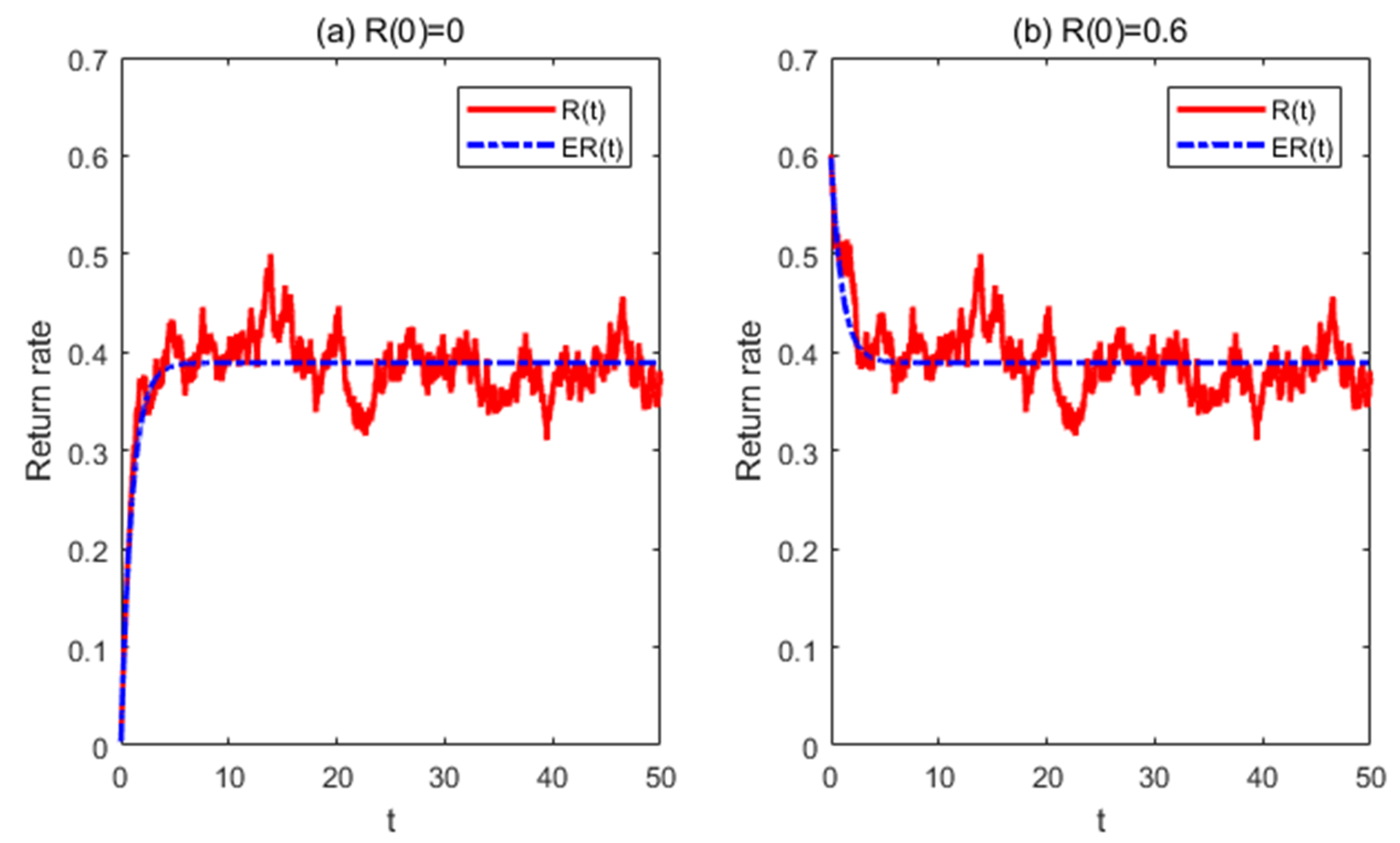
Figure 1 illustrates the evolutionary path of the return rate in the presence of stochastic disturbances. The return rate may increase or decrease over time in terms of expected value. The expectation of the return rate will converge into a stable state along with time, whatever the initial return rate is. The optimal strategy for the retailer is to keep the system state as close as possible to the stable state, even though the initial return rate is above the stable state. The return rate always hovers around its expectation as a result of the stochastic disturbance.
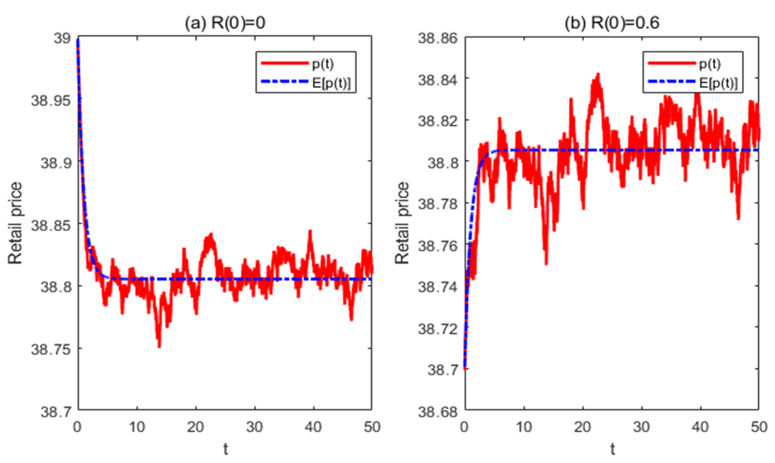
Figure 2 demonstrates the corresponding evolutionary path of the retail price with time. As the retail price is inversely proportional to the return rate, the evolutionary path of the retail price is inverse to the evolutionary path of the return rate. Similarly, the retail price will converge into a stable state in terms of the expectation.
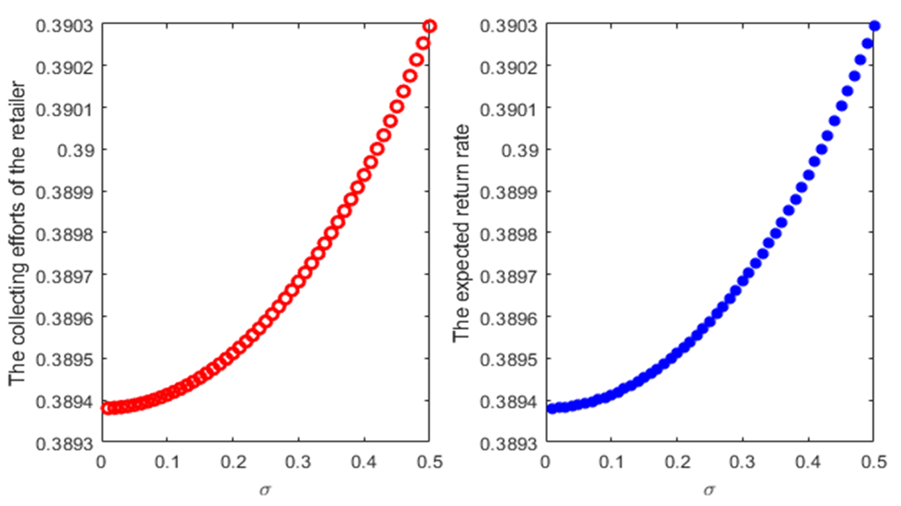
Figure 3 shows the impact of disturbance intensity on the collecting efforts as well as the return rate. The retailer will raise its collecting effort level when the stochastic disturbance intensity is increasing. As a result, the corresponding expected return rate will increase with the increasing of collecting effort. We can expect that the profit rate of the supply chain members will benefit from the increasing of stochastic disturbance intensity. This may come from that the retailer has to raise its collecting effort level to avoid the return rate deviated too far from the stable state, which results in a higher return rate, a lower retail price for the closed-loop supply chain system, and thus a higher profit rate for the supply chain members. However, it should be noticed that this effect is not that prominent which could infer from the increment value.
4. Equilibrium Strategies with Fairness Concern Models
In this section, we will deal with the equilibrium strategies for the supply chain members with the retailer being concerned with fairness. We consider two types of fairness concern retailer, i.e., the gap fairness concern retailer in Section 4.1 (GF model) and self-due fairness concern retailer in Section 4.2 (SF model). We will use these theoretical results to discuss the impact of fairness on the closed-loop supply chain.
4.1. GF Model: Gap Fairness Concern
The unfair feeling of gap fairness concern retailer comes from the profit gap between the retailer and the manufacturer. The retailer considers unfair when the profit the manufacturer earns is more than that the retailer earns, and the more the profit gap, the more unfairness the retailer will think. The gap fairness concern model is similar to Nie and Du [29], Li and Li [31]. Assuming the manufacturer to be fairness neutral, the objective function of the manufacturer is given by
The retailer considers not only about its own profits but also the profit gap between his profit and the manufacturer’s, thus the objective function is formulated by
where represents the fairness concern parameter for the retailer, and the larger it is, the more the retailer is concerned about the fairness of supply chain distribution. The feeling of unfairness comes from the profit gap between the manufacturer’s and the retailer, i.e., . The greater the gap, the more the retailer fells unfairness. Following the same method, we derive the equilibrium strategy for the supply chain members in Proposition 3. The proof of Proposition 3 and 4 are put in the Appendix A.
Proposition 3.
When , GF model exists only one feedback Stackelberg Markov equilibrium. The equilibrium wholesale price is calculated by
The equilibrium retail price is
The equilibrium collecting control strategy is
where
It is shown in Proposition 3 that the presence of gap fairness concern does not affect the existence of Markov equilibrium. The retailer would make his responses according to his feeling about fairness. However, the equilibrium strategies of the retailer are not going to be altered as the manufacturer has taken the retailer’s concern of fairness into consideration. The manufacturer will shift profit to the retailer by way of turning down the wholesale price.
Proposition 4.
In model GF, the expected evolutionary path of return rate is calculated by,
The long-run stable expected return rate can be calculated as,
where
4.2. SF Model: Self-Due Fairness Concern
Unlike the gap fairness concern retailer, the self-due fairness concern retailer takes self-due as the fairness reference point. When the profit the retailer earns in the supply chain is above at the reference point, the retailer considers it is fairness; otherwise if the retailer’s profit is below the reference point, the retailer fells unfairness. Following Du et al. [27], we incorporate the Nash bargaining point as the self-due reference point for the retailer. As such, the retailer takes the Nash bargaining point to be a fairness distribution between the supply chain members. Also, assuming the manufacturer to be fairness neutral, we formulate the objective function of the manufacturer as
Taking the Nash bargaining point as the self-due fairness reference point, the objective function of the retailer in model SF is formulated as
In which is the Nash bargaining profit for the retailer. Denote as the Nash bargaining power parameter for the retailer, the Nash bargaining point is calculated in the following.
Lemma 1.
Suppose the manufacturer is fairness neutral, and the retailer is fairness concern with fairness concern parameter, the Nash bargaining reference point for the retailer is given by
Proof.
Because of fairness neutral, the utility rate at time for the manufacturer is . As a result of fairness concern, the utility rate for the retailer is . According to Nash bargaining theory, the Nash bargaining point can be solved by maximizing the Nash product , i.e.,
The Nash bargaining reference point can be solved as □
Substituting the Nash bargaining reference point, the objective for the retailer is
which could be rewrite as
In the Nash bargaining point, the retailer is supposed to take from the distribution. However, the retailer actually gets as a result of the manufacturer takes the distribution power in the channel. The difference is , thus when term is above zero, the retailer will be happy to get more, however, when this term is below zero, the retailer fells unfairness as the profit he earns is less than his self-due profit. The proof of Proposition 5, 6, and 7 are put in the Appendix A.
Proposition 5.
When , SF model exists only one feedback Stackelberg Markov equilibrium. The equilibrium wholesale price is calculated by
The equilibrium retail price is
The equilibrium collecting control strategy is
where
Once again, the presence of self-due fairness concern would not affect the existence of Markov equilibrium. From Proposition 3 and 5, we could conclude that the preference of fairness concern of the retailer would not affect the existence of equilibrium and the equilibrium strategies of the retailer, whatever the type of fairness concern is. The manufacturer confronts the self-due fairness concern retailer will choose his wholesale price according to the channel power of the retailer and the fairness concern degree of the retailer.
Proposition 6.
In model SF, the expected evolutionary path of return rate is calculated by,
The long-run stable expected return rate can be calculated as,
whereWe conclude in Proposition 7 with the impact of fairness concern on the feedback control strategies for the retailer.
Proposition 7.
For the same return rate, the retailers with different fairness concern type make the same feedback control strategies, i.e.,
Proposition 7 indicates that whether gap fairness concern or self-due fairness concern would not affect the equilibrium feedback control strategies, in terms of retail price and collecting effort. The retailers with different fairness type will make strategy according to his fairness concern type and the manufacturer’s wholesale price. However, as the manufacturer takes the social preference of fairness concern into consideration, the retailer would not change his equilibrium strategies compared to no fairness concern. This means the manufacturer has to shift profit to the retailer in the presence of fairness concern for the follower. Otherwise, the supply chain system could make even less profit rate compared to the system with no fairness concern retailer.
5. Numerical Analysis between Different Fairness Type
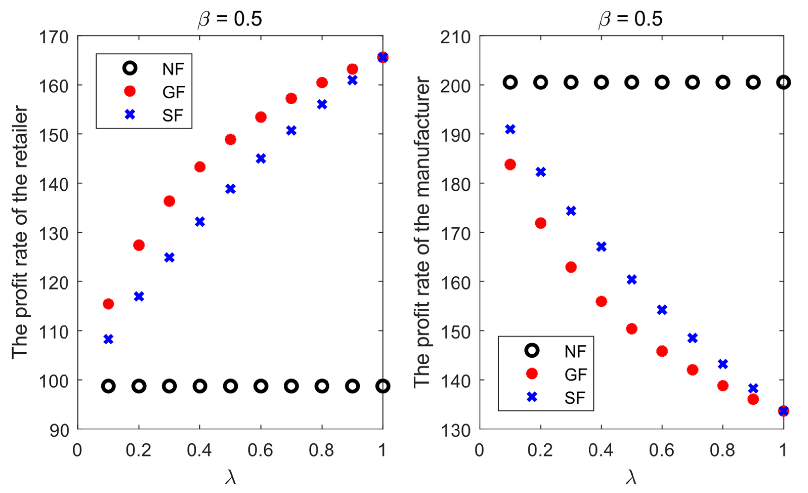
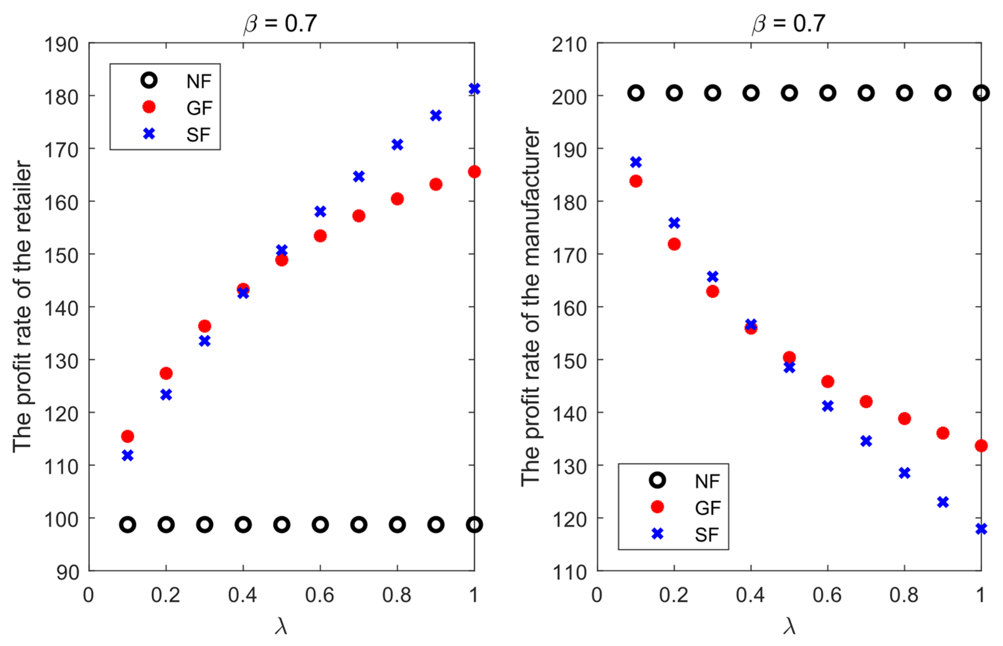
In this section, we would investigate how the manufacturer would shift profit to the retailer according to different fairness concern type for the retailer. The approximation is the same as that used in 3.3. We compare the expected long-run equilibrium profit rate for the manufacturer and the retailer in Figure 4, Figure 5 and Figure 6. Figure 4 shows the comparison results of , which represents the scenario in which the Nash bargaining power is small for the retailer. Thus Figure 5 and Figure 6 represent the scenario with equal Nash bargaining power and high Nash bargaining power, respectively.
Figure 4, Figure 5 and Figure 6 illustrate that the more the retailer concerns about fairness, the more profit the manufacturer will shift to the retailer, irrespective of whether the retailer is gap fairness concern or self-due fairness concern. When the retailer is gap fairness concern, the profit rate of the retailer will increase over the fairness concern degree faster than the self-due fairness concern, which makes the gap fairness concern retailer an aggressive fairness concern type.
Figure 4 and Figure 5 demonstrate that gap fairness concern can bring more profit shifting for the retailer when the Nash bargaining power of the retailer is below 0.5. When the Nash bargaining power of the retailer is above 0.5, self-due fairness concern may bring more profit shifting for the retailer. In model SF, the retailer sets the fairness reference point by Nash bargaining point, according to his bargaining power. The retailer can accept low distribution when his channel power is small, and he will request more distribution as his channel power is rising to large. Basically, the self-due fairness concern retailer expresses his feeling of unfairness by way of Nash bargaining point. It is seemed to be quite reasonable for both the retailer and the manufacturer.
In contrast, gap fairness concern retailer is more aggressive when his channel power is low and conservative when his channel power is rising to large. Although the gap fairness concern may bring more profit shifting for the retailer when his channel power is low, it may incur the dislike of the manufacturer, who thought the retailer may be too greedy and thus may decide not to consider the feeling of the unfairness of the retailer.
Thus, we conclude that the type of self-due fairness concern is more reasonable for the retailer to express its concern of fairness, and is more acceptable for the manufacturer to consider its profit shifting for the retailer.
6. Coordinate Contract
In this section, we first discuss the optimal control strategy for the centralized closed-loop supply chain, and then design a coordinate contract for the manufacturer to coordinate with the retailer. Utilizing superscript and to represent the centralized model and coordinated model in the following.
6.1. Centralized Model
In the centralized supply chain, there is only one decision-maker who decides both the retail price as well as the collecting effort, simultaneously. The objective function for the centralized decision maker is formulated by
The proof for Proposition 8 can be found in the Appendix A.
Proposition 8.
When , the optimal feedback control strategies for the centralized model is calculated by
The value function for the supply chain is
where
It is obvious that the retail price is lower and the collecting effort is larger in the centralized model, compared with that in the decentralized models. The double marginalization effect appears both in the forward channel and the reverse channel of the closed-loop supply chain. The double marginalization effect in the forward channel is quite common in the management literature. The reverse side double marginalization effect mainly comes from that the retailer will choose his collecting effort according to the marginal value of the return rate to his value function, not according to the total marginal value of the supply chain members.
6.2. Coordinate Contract
To coordinate the supply chain, there are two parts needed to be considered, i.e., the revenue of selling the new products and the expenditure of collecting the used-products. As the optimal collecting effort of the retailer is always , it is impossible to coordinate the supply chain unless the manufacturer shares cost expenditure for the retailer. That is to say, suppose in the coordinated model, the collecting effort must satisfy . As such, the closed-loop supply chain cannot be coordinated by the traditional two-part tariff or revenue sharing contract. We designed a hybrid contract to coordinate the supply chain in the following Proposition 9. Suppose the reservation value for the retailer is . The problem can be summarized as
Proposition 9.
A hybrid contract can coordinate the supply chain. The wholesale price of the manufacturer is
The collecting expenditure sharing ratio of the manufacturer is
The franchise fee of the retailer is
The value functions of the manufacturer and the retailer in the coordinated model are
Proof.
The HJB equation of the retailer is
The optimal response is
According to , we derive
The HJB equation of the manufacturer is
Substituting the optimal responses of the retailer into the HJB equation of the manufacturer and taking the first-order condition yields
Thus, the optimal strategy for the retailer is
Now the HJB equation for the manufacturer is
To coordinate the supply chain, we must have
That is to say
We have right now
Assuming , =, we can derive that , . □
The wholesale price in the coordinated contract is precisely the marginal cost for the manufacturer, which equals the unit production cost minus the cost saving from making use of the returned used-products. The collecting expenditure sharing percentage is the ratio of the marginal value of the retailer to the total marginal value of the supply chain members. It indicates that the retailer will only be willing to making the effort which is in direct proportion to his return rate marginal value. Only when the manufacturer undertakes the collecting expenditure which is relevant to his return rate marginal value, the supply chain can be coordinated.
7. Conclusions
This paper addresses the stochastic collecting control problem in a closed-loop supply chain consisting of one manufacturer and one retailer, concerned with fairness. Stochastic differential game models are formulated to discuss the optimal return problem with dynamic characteristics and random disturbance, and the feedback equilibriums are resolved by the HJB equation method. We also derived the evolutionary path of the return rate under the equilibrium control strategies for different models with different fairness concern types. Furthermore, we designed a coordinate contract for the manufacturer to coordinate with the retailer.
We have found that only under a specific condition there exists a unique feedback Markov equilibrium for the closed-loop supply chain. The conditions of the existence for the decentralized supply chain models are the same, whatever the fairness concern type the retailer is. The equilibrium wholesale price and retail price strategies decrease over the return rate, and the equilibrium collecting control strategy increases over the return rate. The evolutionary path of the return rate cannot be predicted precisely because of the stochastic disturbance in the collecting process. We derived the expectation of the stochastic return rate that approaches a stable state along with the time. The monotonicity of the expectation is relevant to the initial value of the return rate, and whatever the initial return rate is, the expectation approaches the same stable state for a CLSC system. The manufacturer and the retailer can benefit from the increasing of disturbance intensity, although the effect is not that obvious in terms of profit increment.
We further investigate how the presence of fairness concern for the retailer would affect the supply chain system. We derived the feedback equilibriums with two fairness concern types of the retailer, i.e., the gap fairness concern retailer and the self-due fairness concern retailer. The results indicate that whether gap fairness concern or self-due fairness concern would not affect the equilibrium feedback control strategies, in terms of retail price and collecting effort. The manufacturer has to shift profit to the retailer in the presence of fairness concern for the follower. The gap fairness concern retailer is more aggressive when his channel power is low and conservative when his channel power is rising to large. In contrast, the type of self-due fairness concern is more reasonable for the retailer to express its concern of fairness and is more acceptable for the manufacturer to consider its profit shifting for the retailer.
We found the traditional two-part tariff or the revenue sharing contract is not able to coordinate the closed-loop supply chain. We designed a hybrid contract with wholesale price, franchise fee and collecting expenditure sharing for the manufacturer to coordinate with the retailer. The collecting expenditure sharing percentage equals the ratio of the marginal value of the retailer to the total marginal value of the supply chain members.
The managerial implications for the supply chain members are as follows. From the long-run perspective, the manufacturer who leads the CLSC should shift some revenue to the retailer who are engaged in the used-products collecting, in order to relieve the fairness concern of the retailer. The retailer acts as a gap fairness concern type would be too aggressive while self-due fairness concern type would be more reasonable for both the manufacturer and the retailer to accept the fairness appeal. Although the manufacturer cannot simply adopt a two-party tariff or a revenue sharing contract to coordinate the CLSC, the manufacturer could employ the hybrid contract to coordinate the CLSC.
There are several limitations to this research. First, because of the complexity of the stochastic differential game model, we did not study the CLSC scenario with competing retailers. However, the competing retailers are more usual in a supply chain with the manufacturer being a leader. Moreover, the presence of competition would bring the peer-induced fairness problem. Therefore, it would be interesting how the presence of competition, as well as peer-induced fairness concern, would co-affect the equilibrium strategies as well as the stable state for the system. Second, we only consider that the retailer collects the used-product on his own. However, the manufacturer could employ some incentive programs to better motivate the retailer on used-product collection. As such, what kind of incentive program should be adopted for the manufacturer and what is the effect of the incentive program on the system return rate and profit of the supply chain members would be meaningful questions.
Funding
This research was partially funded by National Natural Science Foundation of China with grant number 71602116, Science and Technology Ministry of China for Cruise Program under grant number 2018-473, and Doctoral Fund of Ministry of Education of China with grant number 2017M62137.
Conflicts of Interest
The authors declare no conflict of interest.
Appendix A
Proof of Proposition 3. In model GF, the Hamilton–Jacobi–Bellman equation for the retailer is formulated by
The best response of the retailer can be resolved by the first-order condition as
The HJB equation of the manufacturer can be formulated by
Inserting the best response of the retailer into the value function of the manufacturer, we obtain the optimal wholesale price control strategy as
Thus, the equilibrium control strategy of the retailer is derived as
Following the same procedure, the value functions of the manufacturer and the retailer are conjectured as: and . The coefficients are calculated by
Proof of Proposition 4. In model GF, take the equilibrium collecting strategy into Equation (1),
Denote , and let , thus
Make use of the stochastic integral equation and take the expectation,
The above equation can be solved as the same way of Proposition 2, then the result is
Similarly, assume to ensure that the long-run return rate is smaller than 1.
Proof of Proposition 5. The procedure is quite similar with the proof of Proposition 1 and 3. We omit it here.
References
- Qiang, Q.P. The closed-loop supply chain network with competition and design for remanufactureability. J. Clean. Prod. 2015, 105, 348–356. [Google Scholar] [CrossRef]
- Savaskan, R.C.; Van Wassenhove, L.N. Reverse channel design: The case of competing retailers. Manag. Sci. 2006, 52, 1–14. [Google Scholar] [CrossRef] [Green Version]
- Qiang, Q.; Ke, K.; Anderson, T.; Dong, J. The closed-loop supply chain network with competition, distribution channel investment, and uncertainties. Omega 2013, 41, 186–194. [Google Scholar] [CrossRef]
- Shi, J.; Zhang, G.; Sha, J. Optimal production planning for a multi-product closed loop system with uncertain demand and return. Comput. Oper. Res. 2011, 38, 641–650. [Google Scholar] [CrossRef] [Green Version]
- Tan, Y.; Guo, C. Research on Two-Way Logistics Operation with Uncertain Recycling Quality in Government Multi-Policy Environment. Sustainability 2019, 11, 882. [Google Scholar] [CrossRef] [Green Version]
- Huang, Z.; Nie, J.; Tsai, S.B. Dynamic collection strategy and coordination of a remanufacturing closed-loop supply chain under uncertainty. Sustainability 2017, 9, 683. [Google Scholar] [CrossRef] [Green Version]
- Cao, J.; Chen, X.; Zhang, X.; Gao, Y.; Zhang, X.; Kumar, S. Overview of remanufacturing industry in China: Government policies, enterprise, and public awareness. J. Clean. Prod. 2020, 242, 118450. [Google Scholar] [CrossRef]
- Fehr, E.; Schmidt, K.M. A theory of fairness, competition, and cooperation. Q. J. Econ. 1999, 114, 817–868. [Google Scholar] [CrossRef]
- Cui, T.H.; Raju, J.S.; Zhang, Z.J. Fairness and channel coordination. Manag. Sci. 2007, 53, 1303–1314. [Google Scholar]
- Loch, C.H.; Wu, Y. Social preferences and supply chain performance: An experimental study. Manag. Sci. 2008, 54, 1835–1849. [Google Scholar] [CrossRef] [Green Version]
- Ho, T.H.; Su, X. Peer-induced fairness in games. Am. Econ. Rev. 2009, 99, 2022–2049. [Google Scholar] [CrossRef] [Green Version]
- Atasu, A.; Sarvary, M.; Van Wassenhove, L.N. Remanufacturing as a marketing strategy. Manag. Sci. 2008, 54, 1731–1746. [Google Scholar] [CrossRef] [Green Version]
- Govindan, K.; Soleimani, H.; Kannan, D. Reverse logistics and closed-loop supply chain: A comprehensive review to explore the future. Eur. J. Oper. Res. 2015, 240, 603–626. [Google Scholar] [CrossRef] [Green Version]
- Govindan, K.; Soleimani, H. A review of reverse logistics and closed-loop supply chains: A Journal of Cleaner Production focus. J. Clean. Prod. 2017, 142, 371–384. [Google Scholar] [CrossRef]
- Savaskan, R.C.; Bhattacharya, S.; Van Wassenhove, L.N. Closed-loop supply chain models with product remanufacturing. Manag. Sci. 2004, 50, 239–252. [Google Scholar] [CrossRef] [Green Version]
- Huang, M.; Song, M.; Lee, L.H.; Ching, W.K. Analysis for strategy of closed-loop supply chain with dual recycling channel. Int. J. Prod. Econ. 2013, 144, 510–520. [Google Scholar] [CrossRef]
- De Giovanni, P.; Zaccour, G. A two-period game of a closed-loop supply chain. Eur. J. Oper. Res. 2014, 232, 22–40. [Google Scholar] [CrossRef]
- Jacobs, B.W.; Subramanian, R. Sharing responsibility for product recovery across the supply chain. Prod. Oper. Manag. 2012, 21, 85–100. [Google Scholar] [CrossRef]
- Subramanian, R.; Gupta, S.; Talbot, B. Product design and supply chain coordination under extended producer responsibility. Prod. Oper. Manag. 2009, 18, 259–277. [Google Scholar] [CrossRef]
- Jena, S.K.; Sarmah, S.P. Price competition and co-operation in a duopoly closed-loop supply chain. Int. J. Prod. Econ. 2014, 156, 346–360. [Google Scholar] [CrossRef]
- Zu-Jun, M.; Zhang, N.; Dai, Y.; Hu, S. Managing channel profits of different cooperative models in closed-loop supply chains. Omega 2016, 59, 251–262. [Google Scholar] [CrossRef]
- Guide, V.D.R., Jr.; Van Wassenhove, L.N. Managing product returns for remanufacturing. Prod. Oper. Manag. 2001, 10, 142–155. [Google Scholar] [CrossRef]
- Nakashima, K.; Arimitsu, H.; Nose, T.; Kuriyama, S. Optimal control of a remanufacturing system. Int. J. Prod. Res. 2004, 42, 3619–3625. [Google Scholar] [CrossRef] [Green Version]
- Fallah, H.; Eskandari, H.; Pishvaee, M.S. Competitive closed-loop supply chain network design under uncertainty. J. Manuf. Syst. 2015, 37, 649–661. [Google Scholar] [CrossRef]
- De Giovanni, P.; Zaccour, G. Cost–Revenue Sharing in a Closed-Loop Supply Chain; Advances in Dynamic Games; Birkhäser: Boston, MA, USA, 2013; pp. 395–421. [Google Scholar]
- De Giovanni, P.; Reddy, P.V.; Zaccour, G. Incentive strategies for an optimal recovery program in a closed-loop supply chain. Eur. J. Oper. Res. 2016, 249, 605–617. [Google Scholar] [CrossRef]
- Caliskan-Demirag, O.; Chen, Y.F.; Li, J. Channel coordination under fairness concerns and nonlinear demand. Eur. J. Oper. Res. 2010, 207, 1321–1326. [Google Scholar] [CrossRef]
- Du, S.; Nie, T.; Chu, C.; Yu, Y. Newsvendor model for a dyadic supply chain with Nash bargaining fairness concerns. Int. J. Prod. Econ. 2014, 52, 5070–5085. [Google Scholar] [CrossRef]
- Ho, T.H.; Su, X.; Wu, Y. Distributional and peer-induced fairness in supply chain contract design. Prod. Oper. Manag. 2014, 23, 161–175. [Google Scholar] [CrossRef] [Green Version]
- Nie, T.; Du, S. Dual-fairness supply chain with quantity discount contracts. Eur. J. Oper. Res. 2017, 258, 491–500. [Google Scholar] [CrossRef]
- Shu, Y.; Dai, Y.; Ma, Z. Pricing Decisions in Closed-Loop Supply Chains with Peer-Induced Fairness Concerns. Sustainability 2019, 11, 5071. [Google Scholar] [CrossRef] [Green Version]
- Xiao, J.; Huang, Z. A Stochastic Differential Game in the Closed-Loop Supply Chain with Third-Party Collecting and Fairness Concerns. Sustainability 2019, 11, 2241. [Google Scholar] [CrossRef] [Green Version]
- Li, T.; Xie, J.; Zhao, X.; Tang, J. On supplier encroachment with retailer’s fairness concerns. Comput. Ind. Eng. 2016, 98, 499–512. [Google Scholar] [CrossRef]
- Li, Q.H.; Li, B. Dual-channel supply chain equilibrium problems regarding retail services and fairness concerns. Appl. Math. Model. 2016, 40, 7349–7367. [Google Scholar] [CrossRef]
Figure 1.
The evolutionary path of return rate with different initial values.

Figure 2.
The evolutionary path of retail price with different initial values.

Figure 3.
The impact of disturbance intensity on the collecting efforts and return rate.

Figure 4.
The comparison of profit rate for the supply chain members when .

Figure 5.
The comparison of profit rate for the supply chain members when .

Figure 6.
The comparison of profit rate for the supply chain members when .


Table 1.
Notations throughout the paper.
| Notation | Definition |
|---|---|
| Unit production cost of product with raw material and used products | |
| Unit cost savings from remanufacturing | |
| Return rate of used products at time | |
| Collecting effort of the retailer at time | |
| , | Wholesale price and retail price of product at time |
| Demand rate of product | |
| Unit subsidy manufacturer gives to retailer for collecting used products | |
| Scaling parameter of collecting cost function | |
| Effect of collecting efforts on return rate | |
| Decaying rate of return rate | |
| Variance of the stochastic disturbance | |
| Standard Wiener process | |
| Standard normal random variables | |
| Market potential of product | |
| Elasticity of demand with respect to price | |
| Discount rate for decision makers | |
| Fairness concern parameter and Nash bargaining parameter of retailer | |
| Profit rate and utility rate of player at time , represent manufacturer and retailer | |
| , | Objective function and value function for player under the model , where and |
© 2020 by the author. Licensee MDPI, Basel, Switzerland. This article is an open access article distributed under the terms and conditions of the Creative Commons Attribution (CC BY) license (http://creativecommons.org/licenses/by/4.0/).
Share and Cite
MDPI and ACS Style
Huang, Z. Stochastic Differential Game in the Closed-Loop Supply Chain with Fairness Concern Retailer. Sustainability 2020, 12, 3289. https://doi.org/10.3390/su12083289
AMA Style
Huang Z. Stochastic Differential Game in the Closed-Loop Supply Chain with Fairness Concern Retailer. Sustainability. 2020; 12(8):3289. https://doi.org/10.3390/su12083289
Chicago/Turabian StyleHuang, Zongsheng. 2020. "Stochastic Differential Game in the Closed-Loop Supply Chain with Fairness Concern Retailer" Sustainability 12, no. 8: 3289. https://doi.org/10.3390/su12083289
Note that from the first issue of 2016, this journal uses article numbers instead of page numbers. See further details here.